The Dissertation Committee for Nikhil Ulhas Kundargi
certifies that this is the approved version of the following dissertation:
Novel Channel Sensing and Access Strategies in
Opportunistic Spectrum Access Networks
Committee:
Ahmed Tewfik, Supervisor
Jeffrey Andrews
Lili Qiu
Sujay Sanghavi
Sriram Vishwanath

Novel Channel Sensing and Access Strategies in
Opportunistic Spectrum Access Networks
by
Nikhil Ulhas Kundargi, B.E.
Dissertation
Presented to the Faculty of the Graduate School of
The University of Texas at Austin
in Partial Fulfillment
of the Requirements
for the Degree of
DOCTOR OF PHILOSOPHY
THE UNIVERSITY OF TEXAS AT AUSTIN
May 2012

Acknowledgments
It is a pleasure to thank those who have made this thesis possible. First and foremost,
I am greatly privileged to have worked with my adviser Professor Ahmed Tewfik. He instilled
in me the joy of being a researcher. I owe a great debt of gratitude for his insightful mentoring,
constant encouragement, and farsighted guidance. I am grateful to my doctoral committee
members Prof. Jeffrey Andrews, Prof. Sriram Vishwanath, Prof. Sujay Sanghavi and
Prof. Lili Qiu for their helpful and constructive inputs to this thesis. I would also like
to thank my qualifying examination committee members at the University of Minnesota,
Prof. Nihar Jindal, Prof. Emad Ebbini, Prof. Douglas Hawkins, Prof. Mostafa Kaveh and
Prof. Tian He for their help in formulating the thesis. I am grateful to my colleagues at
National Instruments and Qualcomm during my internships for their insights into modern
telecommunications industry, especially Sam Shearman. Also, I am thankful to my colleague
Yingxi for his companionship during countless hours of brainstorming. My senior labmates
Vikrham, Seshan, Cheolhong have made it easier for me to follow in their footsteps and Dan,
Youngchun, Vimal, Vijay, Neeraj, Rahul, Mostafa, Brice, Guido have been great colleagues.
My PhD buddies Ajay, Devdatta, Salil B, Shruti P, Esha have shared their war stories to
keep me going. My friends Shruti K, Sajal, Siddharth, Neha, Raghav, Harsh, Pranav B,
Pranav K, Anush, Nikhil G, Salil V, Purva, Sudarshan, Madhura, Rahul, Anuj, Nachiket,
Khushbu, Sandeep and countless others have lightened my burden and made the last few
years some of the most enjoyable ones of my life. My undergraduate friends Anup, Amogh,
Kaustubh, Harshad, Neil inspired me to pursue this path. Lastly and most importantly, I
am indebted to my parents and to my sister for being extremely supportive of my graduate
studies.
iii

Novel Channel Sensing and Access Strategies in
Opportunistic Spectrum Access Networks
Nikhil Ulhas Kundargi, Ph.D.
The University of Texas at Austin, 2012
Supervisor: Ahmed Tewfik
Traditionally radio spectrum was considered a commodity to be allocated in a fixed
and centralized manner, but now the technical community and the regulators approach it as
a shared resource that can be flexibly and intelligently shared between competing entities.
In this thesis we focus on novel strategies to sense and access the radio spectrum within
the framework of Opportunistic Spectrum Access via Cognitive Radio Networks (CRNs).
In the first part we develop novel transmit opportunity detection methods that effectively
exploit the gray space present in packet based networks. Our methods proactively detect the
maximum safe transmit power that does not significantly affect the primary network nodes
via an implicit feedback mechanism from the Primary network to the Secondary network. A
novel use of packet interarrival duration is developed to robustly perform change detection
in the primary network’s Quality of Service. The methods are validated on real world IEEE
802.11 WLANs. In the second part we study the inferential use of Goodness-of-Fit tests for
spectrum sensing applications. We provide the first comprehensive framework for decision
fusion of an ensemble of goodness-of-fit tests through use of p-values. Also, we introduce a
generalized Φ-divergence statistic to formulate goodness-of-fit tests that are tunable via a
single parameter. We show that under uncertainty in the noise statistics or non-Gaussianity
in the noise, the performance of such non-parametric tests is significantly superior to that of
iv

conventional spectrum sensing methods. Additionally, we describe a collaborative spatially
separated version of the test for robust combining of tests in a distributed spectrum sensing
setting. In the third part we develop the sequential energy detection problem for spectrum
sensing and formulate a novel Sequential Energy Detector. Through extensive simulations we
demonstrate that our doubly hierarchical sequential testing architecture delivers a significant
throughput improvement of 2 to 6 times over the fixed sample size test while maintaining
equivalent operating characteristics as measured by the Probabilities of Detection and False
Alarm. We also demonstrate the throughput gains for a case study of sensing ATSC television
signals in IEEE 802.22 systems.
v
Table of Contents
Acknowledgments iii
Abstract iv
List of Figures x
Chapter 1. Introduction 1
1.1 Spectrum Availability and Spectrum Utilization . . . . . . . . . . . . . . . . 1
1.2 Cognitive Radio . . . . . . . . . . . . . . . . . . . . . . . . . . . . . . . . . . 3
1.2.1 Definitions . . . . . . . . . . . . . . . . . . . . . . . . . . . . . . . . . 31.3 Opportunistic Spectrum Access . . . . . . . . . . . . . . . . . . . . . . . . . 5
1.3.1 Key Terms . . . . . . . . . . . . . . . . . . . . . . . . . . . . . . . . . 6
1.4 Organization . . . . . . . . . . . . . . . . . . . . . . . . . . . . . . . . . . . . 8
Chapter 2. Proactive Identification and Utilization of Transmission Oppor-tunities 11
2.1 Introduction . . . . . . . . . . . . . . . . . . . . . . . . . . . . . . . . . . . . 112.2 Background . . . . . . . . . . . . . . . . . . . . . . . . . . . . . . . . . . . . 14
2.2.1 Change Detection Based Methods . . . . . . . . . . . . . . . . . . . . 14
2.2.2 Estimation of Network Parameters . . . . . . . . . . . . . . . . . . . . 152.2.3 IEEE 802.22 WRAN Standard . . . . . . . . . . . . . . . . . . . . . . 152.2.4 Interference Temperature . . . . . . . . . . . . . . . . . . . . . . . . . 15
2.2.5 SWIFT . . . . . . . . . . . . . . . . . . . . . . . . . . . . . . . . . . . 162.3 Analysis of Network Traffic . . . . . . . . . . . . . . . . . . . . . . . . . . . . 19
2.4 Transmit Margin . . . . . . . . . . . . . . . . . . . . . . . . . . . . . . . . . 20
2.5 Network-level Descriptors . . . . . . . . . . . . . . . . . . . . . . . . . . . . . 21
2.5.1 Primary Network can be characterized through its observable statistics 22
2.5.2 Distribution of Statistics is relatively stationary over short time intervals 22
2.5.3 Changes in QoS of Primary Network are mirrored in its Network Statistics 23
2.6 ProTOMAC: Description and Flowchart . . . . . . . . . . . . . . . . . . . . 24
2.6.1 Secondary Channel Structure . . . . . . . . . . . . . . . . . . . . . . . 25
2.6.1.1 Initialization . . . . . . . . . . . . . . . . . . . . . . . . . . . 262.6.1.2 Channel Access . . . . . . . . . . . . . . . . . . . . . . . . . . 26
vi

2.6.1.3 Transmit Power Control Loop . . . . . . . . . . . . . . . . . . 26
2.6.1.4 Channel Hopping . . . . . . . . . . . . . . . . . . . . . . . . . 27
2.7 Network Descriptors . . . . . . . . . . . . . . . . . . . . . . . . . . . . . . . . 27
2.7.1 Packet Size . . . . . . . . . . . . . . . . . . . . . . . . . . . . . . . . . 272.7.2 Packet Retry Rate . . . . . . . . . . . . . . . . . . . . . . . . . . . . . 30
2.7.3 Channel Interarrival Time . . . . . . . . . . . . . . . . . . . . . . . . . 302.8 Network Statistics Change Detection . . . . . . . . . . . . . . . . . . . . . . 31
2.8.1 Goodness-of-Fit Tests . . . . . . . . . . . . . . . . . . . . . . . . . . . 312.8.2 Implementation of the Kolmogorov-Smirnov test . . . . . . . . . . . . 32
2.8.3 Sequential Kolmogorov-Smirnov Test . . . . . . . . . . . . . . . . . . . 34
2.8.4 Cramer von-Mises GoF Test . . . . . . . . . . . . . . . . . . . . . . . 362.8.5 Anderson-Darling Test and Related Tests . . . . . . . . . . . . . . . . 38
2.8.6 The Parallelized GoF Test . . . . . . . . . . . . . . . . . . . . . . . . . 392.8.7 Kullback-Leibler Divergence . . . . . . . . . . . . . . . . . . . . . . . . 40
2.8.8 Bhattacharyya Distance . . . . . . . . . . . . . . . . . . . . . . . . . . 41
2.8.9 Group Sequential Divergence Updates . . . . . . . . . . . . . . . . . . 42
2.8.9.1 KL Divergence Group Sequential Update . . . . . . . . . . . . 43
2.8.10 Theoretical Performance Bounds . . . . . . . . . . . . . . . . . . . . . 442.9 Density Estimation . . . . . . . . . . . . . . . . . . . . . . . . . . . . . . . . 45
2.9.1 Deheuvel’s Rule of Thumb Method . . . . . . . . . . . . . . . . . . . . 472.10 Experimental Testbed Setup . . . . . . . . . . . . . . . . . . . . . . . . . . . 49
2.10.1 Primary Network Configuration . . . . . . . . . . . . . . . . . . . . . . 49
2.10.2 Secondary Network Configuration . . . . . . . . . . . . . . . . . . . . 50
2.10.3 Implementation Issues . . . . . . . . . . . . . . . . . . . . . . . . . . . 51
2.10.3.1 Study of Network Stationarity . . . . . . . . . . . . . . . . . . 51
2.11 Experimental Results For Goodness of Fit Tests . . . . . . . . . . . . . . . . 52
2.11.1 Sequential Kolmogorov-Smirnov Test . . . . . . . . . . . . . . . . . . . 52
2.11.2 Parallelized Goodness-of-Fit test . . . . . . . . . . . . . . . . . . . . . 562.11.3 Comparison with the SWIFT approach . . . . . . . . . . . . . . . . . 59
2.12 Experimental Results for Divergence Measure based Tests . . . . . . . . . . . 60
2.12.1 Baseline Density Estimates . . . . . . . . . . . . . . . . . . . . . . . . 60
2.12.2 Tests using Randomized Sampling . . . . . . . . . . . . . . . . . . . . 63
2.12.3 Group Sequential Test . . . . . . . . . . . . . . . . . . . . . . . . . . . 63
2.12.4 Secondary Link Power Budget . . . . . . . . . . . . . . . . . . . . . . 64
2.13 Conclusions . . . . . . . . . . . . . . . . . . . . . . . . . . . . . . . . . . . . 65
vii

Chapter 3. Phi-divergence based Ensemble Goodness of Fit tests 69
3.1 Introduction . . . . . . . . . . . . . . . . . . . . . . . . . . . . . . . . . . . . 693.1.1 Our Contributions . . . . . . . . . . . . . . . . . . . . . . . . . . . . . 693.1.2 Related Work . . . . . . . . . . . . . . . . . . . . . . . . . . . . . . . . 71
3.1.2.1 Non Parametric Statistics in Communications . . . . . . . . . 713.1.2.2 Goodness of Fit tests in Cognitive Radio literature . . . . . . 71
3.2 Inference Problem Formulation . . . . . . . . . . . . . . . . . . . . . . . . . . 723.3 Phi-Divergence based Goodness-of-Fit Tests . . . . . . . . . . . . . . . . . . 74
3.3.1 Goodness-of-Fit Procedures . . . . . . . . . . . . . . . . . . . . . . . . 743.3.2 Phi-Divergences . . . . . . . . . . . . . . . . . . . . . . . . . . . . . . 75
3.3.3 Relation of Φ-Divergence Statistics to other Goodness-of-Fit Statistics 76
3.4 Phi-Divergence Tests for Spectrum Sensing . . . . . . . . . . . . . . . . . . . 78
3.4.1 Handling Non-Gaussian Noise . . . . . . . . . . . . . . . . . . . . . . . 78
3.5 Robust Fusion of Goodness of Fit Tests . . . . . . . . . . . . . . . . . . . . . 793.5.1 p-value . . . . . . . . . . . . . . . . . . . . . . . . . . . . . . . . . . . 81
3.5.2 Ensemble of Φ-Divergence Test test . . . . . . . . . . . . . . . . . . . 83
3.5.3 Choice of Ensemble GoF test parameters . . . . . . . . . . . . . . . . 88
3.6 Collaborative Spatially separated Ensemble Goodness-of-Fit Tests . . . . . . 90
3.7 Results . . . . . . . . . . . . . . . . . . . . . . . . . . . . . . . . . . . . . . . 923.7.1 Simulation Scenario . . . . . . . . . . . . . . . . . . . . . . . . . . . . 93
3.7.1.1 Handling Complex Data . . . . . . . . . . . . . . . . . . . . . 93
3.7.1.2 Test Power for individual Goodness-of-Fit test . . . . . . . . . 943.7.2 Ensemble Goodness-of Fit (EG) test based on Φ-Divergences . . . . . 94
3.8 Conclusion . . . . . . . . . . . . . . . . . . . . . . . . . . . . . . . . . . . . . 96
Chapter 4. Sequential Approaches to Spectrum Sensing 97
4.1 Introduction . . . . . . . . . . . . . . . . . . . . . . . . . . . . . . . . . . . . 974.1.1 Related Work . . . . . . . . . . . . . . . . . . . . . . . . . . . . . . . . 974.1.2 Our Contributions . . . . . . . . . . . . . . . . . . . . . . . . . . . . . 98
4.2 Notation and Assumptions . . . . . . . . . . . . . . . . . . . . . . . . . . . . 99
4.3 Review of ED and Sequential Detector . . . . . . . . . . . . . . . . . . . . . 100
4.3.1 Threshold Calculation . . . . . . . . . . . . . . . . . . . . . . . . . . . 1014.3.2 Sequential Probability Ratio Test . . . . . . . . . . . . . . . . . . . . . 101
4.4 SEquential Energy Detector: SEED . . . . . . . . . . . . . . . . . . . . . . . 102
4.4.1 SEED Performance Evaluation . . . . . . . . . . . . . . . . . . . . . . 1044.4.2 Problems with Wald Approximations and the Min-M SEED . . . . . . 106
4.5 Signal Variance Estimation . . . . . . . . . . . . . . . . . . . . . . . . . . . . 106
4.5.1 Sensitivity to Signal Variance Estimate . . . . . . . . . . . . . . . . . 107
4.5.2 Hybrid Iterative Bayesian Estimation of σ2s . . . . . . . . . . . . . . . 108
viii

4.5.2.1 Initialization . . . . . . . . . . . . . . . . . . . . . . . . . . . 1094.5.2.2 Update . . . . . . . . . . . . . . . . . . . . . . . . . . . . . . 109
4.5.2.3 Prediction . . . . . . . . . . . . . . . . . . . . . . . . . . . . . 1104.6 Distributed Sequential Detection . . . . . . . . . . . . . . . . . . . . . . . . . 110
4.6.1 Doubly Sequential Energy Detection (DSED) . . . . . . . . . . . . . . 111
4.7 Termination Criteria at Base Station . . . . . . . . . . . . . . . . . . . . . . 1144.7.1 One Shot Detection . . . . . . . . . . . . . . . . . . . . . . . . . . . . 1144.7.2 First-M-Positive Detection . . . . . . . . . . . . . . . . . . . . . . . . 1144.7.3 Wait-Till-TTh Detection . . . . . . . . . . . . . . . . . . . . . . . . . . 114
4.8 Experimental Results . . . . . . . . . . . . . . . . . . . . . . . . . . . . . . . 115
4.9 Case Study 1- Sequential Sensing applied to the IEEE 802.22 Standard . . . 118
4.9.1 FFT based Pilot Detection of ATSC signals . . . . . . . . . . . . . . . 119
4.9.2 Sequential Sensing of ATSC Pilot . . . . . . . . . . . . . . . . . . . . . 120
4.9.2.1 Preprocessing of ATSC signal captures . . . . . . . . . . . . . 120
4.9.3 Simulation Results . . . . . . . . . . . . . . . . . . . . . . . . . . . . . 1224.10 Conclusion . . . . . . . . . . . . . . . . . . . . . . . . . . . . . . . . . . . . . 123
Chapter 5. Conclusion 127
Appendices 131
Appendix A. Abbreviations 132
Bibliography 136
ix
List of Figures
1.1 Allocation of Spectrum in the United States . . . . . . . . . . . . . . . . . . 2
1.2 Utilization of spectrum in New York and Chicago . . . . . . . . . . . . . . . 4
1.3 Utilization of Spectrum in Paris . . . . . . . . . . . . . . . . . . . . . . . . . 5
2.1 FCC’s Interference Temperature Metric as proposed by the FCC . . . . . . . 17
2.2 Transmit Margin . . . . . . . . . . . . . . . . . . . . . . . . . . . . . . . . . 18
2.3 Decay of time stationarity over consecutive slots of 100 packet arrivals for athreshold of 1.0 . . . . . . . . . . . . . . . . . . . . . . . . . . . . . . . . . . 24
2.4 Dependence of Round-trip delay time and Network Statistics on SecondaryInterference . . . . . . . . . . . . . . . . . . . . . . . . . . . . . . . . . . . . 24
2.7 Experiment TestBed . . . . . . . . . . . . . . . . . . . . . . . . . . . . . . . 29
2.8 Sequential KS Test . . . . . . . . . . . . . . . . . . . . . . . . . . . . . . . . 36
2.9 Ψ(t) for various GoF tests . . . . . . . . . . . . . . . . . . . . . . . . . . . . 37
2.11 KDEs of CAP1 Dataset for increasing Tx Power with full capture duration . 46
2.12 Kernel Density Estimates and Packet Length Histograms for CAP3 Datasetusing Deheuvel’s Method . . . . . . . . . . . . . . . . . . . . . . . . . . . . . 48
2.13 Demonstration of Time Stationarity over Captures for 6 increasing Transmis-sion Power Levels . . . . . . . . . . . . . . . . . . . . . . . . . . . . . . . . . 49
2.14 Packet Size Histograms for 4 Tx Power levels . . . . . . . . . . . . . . . . . . 53
2.15 Empirical CDF (using 40 samples) for Tx power 2.3 mW . . . . . . . . . . . 53
2.16 Empirical CDF (using 40 samples) for Tx power 4.6 mW . . . . . . . . . . . 54
2.17 Sequential Behavior of KS Test Statistic with increasing Sample Size . . . . 56
2.22 Probability of Detection (a) and Probability of False Alarm (b) for the Stu-dent’s t test and the Anderson-Darling test for increasing test sample size. . 61
2.23 ProTOMAC Results for CAP1 Dataset . . . . . . . . . . . . . . . . . . . . . 622.25 ProTOMAC Results for CAP1 Dataset . . . . . . . . . . . . . . . . . . . . . 662.26 Group Sequential Test Performance for CAP1 Dataset using Bhattacharyya
Distance as Metric . . . . . . . . . . . . . . . . . . . . . . . . . . . . . . . . 67
3.1 Φ function plots . . . . . . . . . . . . . . . . . . . . . . . . . . . . . . . . . . 77
3.2 K(u,v) with s= 1/2 . . . . . . . . . . . . . . . . . . . . . . . . . . . . . . . . 80
3.3 K(u,v) with s=1 . . . . . . . . . . . . . . . . . . . . . . . . . . . . . . . . . . 80
3.4 K(u,v) with s=2 . . . . . . . . . . . . . . . . . . . . . . . . . . . . . . . . . . 81
3.5 Distributions of the test statistics for the KL test and Phi-Divergence test . 82
x

3.6 Distribution of p-values under H1 and H0 for SNR = -2 dB, test size = 50 . 84
3.7 Block Diagram of Ensemble Goodness-of-Fit tests using tunable Phi-divergencestatistics . . . . . . . . . . . . . . . . . . . . . . . . . . . . . . . . . . . . . . 85
3.8 Performance of the various tests for test size = 50. Fig 3.8a : PD for Gaussiannoise, Fig 3.8b : PD for Non-Gaussian noise with Γ = 0.5 , Fig 3.8d : PFAfor Gaussian noise, Fig 3.8e : PFA for non-Gaussian noise, Fig 3.8f : PFA forNon-Gaussian noise with Γ = 0.1 . . . . . . . . . . . . . . . . . . . . . . . . 86
3.9 Probability of Detection for the CSS-EG test for N = 50 . . . . . . . . . . . 90
3.10 Probability of False Alarm for the CSS-EG test for N = 50 . . . . . . . . . . 91
4.1 Sample Run of the Sequential Test Statistic . . . . . . . . . . . . . . . . . . 103
4.2 χ2 Distribution Approximation . . . . . . . . . . . . . . . . . . . . . . . . . 104
4.4 SNR vs η for a Pd = 0.95 . . . . . . . . . . . . . . . . . . . . . . . . . . . . 107
4.5 % Deviation in η vs % Deviation in σ2s . . . . . . . . . . . . . . . . . . . . . 108
4.6 The Predicted Distribution of PU SNR values after 10 runs . . . . . . . . . . 1084.7 Plot of E[Zk] vs SNR (linear scale) . . . . . . . . . . . . . . . . . . . . . . . 112
4.8 Behavior of PD and PFA vs SNR for SED Test . . . . . . . . . . . . . . . . . 115
4.9 Behavior of PD and PFA vs SNR for DSED Test . . . . . . . . . . . . . . . . 116
4.10 Distribution of Termination Time for SED Test . . . . . . . . . . . . . . . . 1174.11 Distribution of Termination Time for DSED Test . . . . . . . . . . . . . . . 1184.12 Spectral Density of an ATSC channel . . . . . . . . . . . . . . . . . . . . . . 121
4.13 Average dwells required for detection of ATSC signal vs SNR . . . . . . . . . 122
4.14 Distribution of the dwells required for sensing . . . . . . . . . . . . . . . . . 123
xi

Chapter 1
Introduction
In this chapter, we will provide a brief introduction to Cognitive Radio Networks and
the philosophy of Opportunistic Spectrum Access and lay the framework in which to under-
stand the contributions of this thesis. The explosive growth of wireless devices, technologies
and services in the civilian and military fields has made radio spectrum into a precious com-
modity. Historically the spectrum regulatory framework has been formulated in a manner
that radio spectrum is treated as a national resource to be licensed out to users by the
government. These licensees are promised exclusive rights to the use of this spectrum and
an unlicensed transmissions by other parties are considered illegal. The finite amount of
available spectrum has resulted in a situation where the innovative wireless services being
proposed have no spectrum available on which they can be deployed.
1.1 Spectrum Availability and Spectrum Utilization
The apparent shortage of spectrum that can be allocated motivated the scientific
community and the regulatory agencies such as the Federal Communications Commission
(FCC) to closely examine the current spectrum utilization. These efforts revealed a surprising
dichotomy between the amount of spectrum that becomes available for licensing on one hand
and the actual utilization of the spectrum that has already been allotted out on the other
hand. In order to illustrate this situation, we will refer to a number of spectrum utilization
studies that have been conducted over the last few years. Figure 1.1 shows the current
1

U.S.
DEPARTMENT OF COMMERC
ENA
TION
AL TELEC
OM
M
UNICATIONS & INFORMATION
AD
MIN
ISTR
ATI
ON
MO
BILE
(AE
RONA
UTIC
AL T
ELEM
ETER
ING
)
S)
5.68
5.73
5.90
5.95
6.2
6.52
5
6.68
56.
765
7.0
7.1
7.3
7.35
8.1
8.19
5
8.81
5
8.96
59.
040
9.4
9.5
9.9
9.99
510
.003
10.0
0510
.110
.15
11.1
7511
.275
11.4
11.6
11.6
5
12.0
5
12.1
0
12.2
3
13.2
13.2
613
.36
13.4
113
.57
13.6
13.8
13.8
714
.014
.25
14.3
5
14.9
9015
.005
15.0
1015
.10
15.6
15.8
16.3
6
17.4
1
17.4
817
.55
17.9
17.9
718
.03
18.0
6818
.168
18.7
818
.919
.02
19.6
819
.80
19.9
9019
.995
20.0
0520
.010
21.0
21.4
521
.85
21.9
2422
.0
22.8
5523
.023
.223
.35
24.8
924
.99
25.0
05
25.0
125
.07
25.2
125
.33
25.5
525
.67
26.1
26.1
7526
.48
26.9
526
.96
27.2
327
.41
27.5
428
.0
29.7
29.8
29.8
929
.91
30.0
UNITEDSTATES
THE RADIO SPECTRUM
NON-GOVERNMENT EXCLUSIVE
GOVERNMENT/ NON-GOVERNMENT SHAREDGOVERNMENT EXCLUSIVE
RADIO SERVICES COLOR LEGEND
ACTIVITY CODE
NOT ALLOCATED RADIONAVIGATION FIXED
MARITIME MOBILEFIXED
MARITIME MOBILE
FIXED
MARITIME MOBILE
Radiolocation RADIONAVIGATION
FIXED
MARITIMEMOBILE
Radiolocation
FIXED
MARITIMEMOBILE
FIXED
MARITIMEMOBILE
AERONAUTICALRADIONAVIGATION
AERO
NAUT
ICAL
RADI
ONAV
IGAT
ION
Aero
naut
ical
Mob
ile
Mar
itime
Radi
onav
igat
ion
(Rad
io Be
acon
s)M
ARIT
IME
RADI
ONAV
IGAT
ION
(RAD
IO B
EACO
NS)
Aero
naut
ical
Radi
onav
igat
ion
(Rad
io Be
acon
s)
3 9 14 19.9
5
20.0
5
30 30 59 61 70 90 110
130
160
190
200
275
285
300
3 kHz 300 kHz
300 kHz 3 MHz
3 MHz 30 MHz
30 MHz 300 MHz
3 GHz
300 GHz
300 MHz
3 GHz
30 GHz
AeronauticalRadionavigation(Radio Beacons)
MARITIMERADIONAVIGATION(RADIO BEACONS)
Aero
naut
ical
Mob
ile
Mar
itime
Radio
navig
ation
(Rad
io Be
acon
s)
AERO
NAUT
ICAL
RADI
ONAV
IGAT
ION
(RAD
IO B
EACO
NS)
AERONAUTICALRADIONAVIGATION(RADIO BEACONS)
AeronauticalMobile
Aero
naut
ical M
obile
RADI
ONAV
IGAT
ION
AER
ONA
UTIC
ALRA
DIO
NAVI
GAT
ION
MAR
ITIM
EM
OBI
LE AeronauticalRadionavigation
MO
BILE
(DIS
TRES
S AN
D CA
LLIN
G)
MAR
ITIM
E M
OBI
LE
MAR
ITIM
EM
OBI
LE(S
HIPS
ONL
Y)
MO
BILE
AERO
NAUT
ICAL
RADI
ONA
VIG
ATIO
N(R
ADIO
BEA
CONS
)
AERO
NAUT
ICAL
RADI
ONAV
IGAT
ION
(RAD
IO B
EACO
NS)
BROADCASTING(AM RADIO)
MAR
ITIM
E M
OBI
LE (T
ELEP
HONY
)
MAR
ITIM
E M
OBI
LE (T
ELEP
HONY
) M
OBI
LE (D
ISTR
ESS
AND
CALL
ING
)
MARITIMEMOBILE
LAND MOBILE
MOBILE
FIXED STAN
DARD
FRE
Q. A
ND T
IME
SIG
NAL
(250
0kHz
)
STAN
DARD
FRE
Q. A
ND T
IME
SIG
NAL
Spac
e Re
sear
ch MARITIMEMOBILE
LAND MOBILE
MOBILE
FIXED
AERO
NAUT
ICAL
MOB
ILE
(R)
STAN
DARD
FRE
Q.
AERO
NAUT
ICAL
MO
BILE
(R)
AERO
NAUT
ICAL
MOB
ILE
(OR)
AERO
NAUT
ICAL
MOB
ILE
(R)
FIXED
MOBILE**
Radio-location
FIXE
DM
OBI
LE*
AMATEUR
FIXE
D
FIXE
D
FIXE
D
FIXED
FIXE
DMARITIMEMOBILE
MO
BILE
*
MO
BILE
*
MO
BILE
STAN
DARD
FRE
Q. A
ND T
IME
SIG
NAL
(500
0 KH
Z)
AERO
NAUT
ICAL
MO
BILE
(R)
AERO
NAUT
ICAL
MO
BILE
(OR)
STAN
DARD
FRE
Q.
Spac
e Re
sear
ch
MOBILE**
AERO
NAUT
ICAL
MO
BILE
(R)
AERO
NAUT
ICAL
MO
BILE
(OR) FIX
ED
MO
BILE
*
BRO
ADCA
STIN
G
MAR
ITIM
E M
OBI
LE
AERO
NAUT
ICAL
MO
BILE
(R)
AERO
NAUT
ICAL
MO
BILE
(OR) FIXE
DM
obile
AMAT
EUR
SATE
LLIT
EAM
ATEU
R
AMAT
EUR
FIXED
Mobile
MAR
ITIM
E M
OBILE
MARITIMEMOBILE
AERO
NAUT
ICAL
MO
BILE
(R)
AERO
NAUT
ICAL
MO
BILE
(OR)
FIX
ED
BRO
ADCA
STIN
G
FIXE
DST
ANDA
RD F
REQ
. AND
TIM
E SI
GNA
L (1
0,00
0 kH
z)ST
ANDA
RD F
REQ
.Sp
ace
Rese
arch
AERO
NAUT
ICAL
MO
BILE
(R)
AMAT
EUR
FIXED
Mobile* AERO
NAUT
ICAL
MO
BILE
(R)
AERO
NAUT
ICAL
MO
BILE
(OR)
FIXE
D
FIXE
DBRO
ADCA
STIN
G
MAR
ITIM
EM
OBI
LE
AERO
NAUT
ICAL
MOB
ILE (R
)
AERO
NAUT
ICAL
MOB
ILE (O
R)
RADI
O AS
TRON
OMY
Mob
ile*
AMAT
EUR
BRO
ADCA
STIN
G
AMAT
EUR
AMAT
EUR
SATE
LLIT
E
Mob
ile*
FIXE
D
BRO
ADCA
STIN
G
STAN
DARD
FRE
Q. A
ND T
IME
SIG
NAL
(15,
000
kHz)
STAN
DARD
FRE
Q.
Spac
e Re
sear
ch
FIXED
AERO
NAUT
ICAL
MO
BILE
(OR)
MAR
ITIM
EM
OBI
LE
AERO
NAUT
ICAL
MO
BILE
(OR)
AERO
NAUT
ICAL
MO
BILE
(R)
FIXE
D
FIXE
D
BRO
ADCA
STIN
G
STAN
DARD
FRE
Q.
Spac
e Re
sear
ch
FIXE
D
MAR
ITIM
E M
OBI
LE
Mob
ileFI
XED
AMAT
EUR
AMAT
EUR
SATE
LLIT
E
BRO
ADCA
STIN
GFI
XED
AERO
NAUT
ICAL
MO
BILE
(R)
MAR
ITIM
E M
OBI
LE
FIXE
DFI
XED
FIXE
D
Mob
ile*
MO
BILE
**
FIXE
D
STAN
DARD
FRE
Q. A
ND T
IME
SIG
NAL
(25,
000
kHz)
STAN
DARD
FRE
Q.
Spac
e Re
sear
ch
LAN
D M
OBI
LEM
ARIT
IME
MO
BILE
LAN
D M
OBI
LE M
OBI
LE**
RAD
IO A
STRO
NOM
YBR
OAD
CAST
ING
MAR
ITIM
E M
OBI
LE L
AND
MO
BILE
FIXE
D M
OBI
LE**
FIXE
D
MO
BILE
**
MO
BILE
FIXE
D
FIXE
D
FIXE
DFI
XED
FIXE
D
LAND
MOB
ILE
MO
BILE
**
AMAT
EUR
AMAT
EUR
SATE
LLIT
E
MO
BILE
LAN
D M
OBI
LE
MO
BILE
MO
BILE
FIXE
D
FIXE
D
MO
BILE
MO
BILE
FIXE
D
FIXE
D
LAN
DM
OBI
LE
LAN
DM
OBI
LE
LAN
DM
OBI
LE
LAND
MO
BILE
Radi
o As
trono
my
RADI
O AS
TRON
OMY
LAND
MO
BILE
FIXE
DFI
XED
MO
BILEMOB
ILE
MOBILE
LAND
MO
BILE
FIXED
LAN
DM
OBI
LE
FIXE
D
FIXE
D
MO
BILE
MOB
ILE
LANDMOBILE AMATEUR
BROADCASTING(TV CHANNELS 2-4)
FIXE
DM
OBI
LE
FIXE
DM
OBI
LE
FIXE
DM
OBI
LEFI
XED
MO
BILE
AERO
NAUT
ICAL
RAD
IONA
VIG
ATIO
N
BROADCASTING(TV CHANNELS 5-6)
BROADCASTING(FM RADIO)
AERONAUTICALRADIONAVIGATION
AERO
NAU
TICA
LM
OBI
LE (R
)
AERO
NAUT
ICAL
MO
BILE
AERO
NAUT
ICAL
MO
BILE
AER
ON
AUTI
CAL
MO
BILE
(R)
AER
ONA
UTI
CAL
MO
BILE
(R)
AERO
NAUT
ICAL
MO
BILE
(R)
MO
BILE
FIX
ED
AMAT
EUR
BROADCASTING(TV CHANNELS 7-13)
MOBILE
FIXED
MOBILE
FIXED
MOBILE SATELLITE
FIXED
MOBILESATELLITE
MOBILE
FIXED
MOBILESATELLITE
MOBILE
FIXE
DM
OBI
LE
AERO
NAUT
ICAL
RAD
IONA
VIG
ATIO
N
STD.
FRE
Q. &
TIM
E SI
GNAL
SAT
. (40
0.1
MHz
)ME
T. SA
T.(S
-E)
SPAC
E RE
S.(S
-E)
Earth
Exp
l.Sa
tellit
e (E
-S)
MO
BILE
SAT
ELLI
TE (E
-S)
FIXE
DM
OBI
LERA
DIO
ASTR
ONOM
Y
RADI
OLO
CATI
ON
Amat
eur
LAND
MO
BILE
MeteorologicalSatellite (S-E)
LAND
MO
BILE
BROA
DCAS
TING
(TV C
HANN
ELS 1
4 - 20
)
BROADCASTING(TV CHANNELS 21-36)
TV BROADCASTINGRAD
IO A
STR
ON
OM
Y
RADI
OLO
CATI
ON
FIXE
D
Amat
eur
AERONAUTICALRADIONAVIGATION
MO
BILE
**FI
XED
AERO
NAUT
ICAL
RADIO
NAVIG
ATION
Radi
oloc
atio
n
Radi
oloc
atio
nM
ARIT
IME
RADI
ONA
VIG
ATIO
N
MAR
ITIM
ERA
DIO
NAVI
GAT
ION
Radi
oloc
atio
n
Radiolocation
Radiolocation
RADIO-LOCATION RADIO-
LOCATION
Amateur
AERO
NAUT
ICAL
RADI
ONAV
IGAT
ION
(Gro
und)
RADI
O-LO
CATI
ONRa
dio-
locat
ion
AERO
. RAD
IO-
NAV.
(Grou
nd)
FIXED
SAT.
(S-E
)RA
DIO-
LOCA
TION
Radio
-loc
ation
FIXED
FIXEDSATELLITE
(S-E)
FIXE
D
AERO
NAUT
ICAL
RAD
IONA
VIG
ATIO
N MO
BILE
FIXE
DM
OBI
LE
RADI
O A
STRO
NOM
YSp
ace
Rese
arch
(Pas
sive)
AERO
NAUT
ICAL
RAD
IONA
VIG
ATIO
N
RADI
O-
LOCA
TIO
NRa
dio-
loca
tion
RADI
ONA
VIG
ATIO
N
Radi
oloc
atio
n
RADI
OLO
CATI
ON
Radi
oloc
atio
n
Radi
oloc
atio
n
Radi
oloc
atio
n
RADI
OLO
CATI
ON
RADI
O-
LOCA
TIO
N
MAR
ITIM
ERA
DIO
NAVI
GAT
ION
MAR
ITIM
ERA
DION
AVIG
ATIO
NM
ETEO
ROLO
GIC
ALAI
DS
Amat
eur
Amat
eur
FIXED
FIXE
DSA
TELL
ITE
(E-S
)M
OBIL
E
FIXE
DSA
TELL
ITE
(E-S
)
FIXE
DSA
TELL
ITE
(E-S
)M
OB
ILE
FIXE
D FIXE
D
FIXE
D
FIXE
D
MOB
ILE
FIXE
DSP
ACE
RESE
ARCH
(E-S
)FI
XED
Fixe
dM
OBIL
ESA
TELL
ITE
(S-E
)FIX
ED S
ATEL
LITE
(S-E
)
FIXED
SAT
ELLIT
E (S
-E)
FIXED
SATE
LLITE
(S-E
)
FIXE
DSA
TELL
ITE
(S-E
)
FIXE
DSA
TELL
ITE
(E-S
)FI
XED
SATE
LLIT
E (E
-S) FIX
EDSA
TELL
ITE(E
-S) FIX
EDSA
TELL
ITE(E
-S)
FIXE
D
FIXE
D
FIXE
D
FIXE
D
FIXE
D
FIXE
D
FIXE
D
MET.
SATE
LLITE
(S-E
)M
obile
Satel
lite (S
-E)
Mob
ileSa
tellite
(S-E
)
Mobil
eSa
tellite
(E-S
)(no
airb
orne)
Mobil
e Sa
tellite
(E-S
)(no
airbo
rne)
Mobil
e Sa
tellite
(S-E
)
Mob
ileSa
tellite
(E-S
)
MOB
ILE
SATE
LLIT
E (E
-S)
EART
H EX
PL.
SATE
LLITE
(S-E
)
EART
H EX
PL.
SAT.
(S-E
)
EART
H EX
PL.
SATE
LLITE
(S-E
)
MET.
SATE
LLITE
(E-S
)
FIXE
D
FIXE
D
SPAC
E RE
SEAR
CH (S
-E)
(dee
p sp
ace
only)
SPAC
E RE
SEAR
CH (S
-E)
AERO
NAUT
ICAL
RADI
ONA
VIG
ATIO
N
RADI
OLO
CATI
ON
Radi
oloc
atio
n
Radi
oloc
atio
n
Radio
locat
ion
Radio
locat
ion
MAR
ITIM
ERA
DIO
NAVI
GAT
ION M
eteo
rolog
ical
Aids
RADI
ONAV
IGAT
ION
RADI
OLO
CATI
ON
Radi
oloc
atio
n
RADI
O-
LOCA
TIO
N
Radio
locati
on
Radio
locat
ionAm
ateu
r
Amat
eur
Amat
eur
Sate
llite
RADI
OLO
CATI
ON
FIXE
D
FIXE
D
FIXED
FIX
EDFIXED
SATELLITE(S-E)
FIXEDSATELLITE
(S-E)
Mobile **
SPAC
E RE
SEAR
CH(P
assiv
e)EA
RTH
EXPL
.SA
T. (P
assiv
e)RA
DIO
ASTR
ONOM
Y
SPAC
ERE
SEAR
CH (P
assiv
e)EA
RTH
EXPL
.SA
TELL
ITE
(Pas
sive)
RADI
OAS
TRO
NOM
Y
BRO
ADCA
STIN
GSA
TELL
ITE
AERO
NAUT
ICAL
RAD
IONA
V.Sp
ace
Rese
arch
(E-S
)
SpaceResearch
Land
Mob
ileSa
tellite
(E-S
)
Radio
-loc
ation
RADI
O-LO
CATI
ON
RADI
ONA
VIGA
TION FI
XE
DSA
TELL
ITE
(E-S
)La
nd M
obile
Sate
llite
(E-
S)
Land
Mob
ileSa
tellite
(E-S
)Fi
xed
Mob
ileFI
XED
SAT
. (E-
S)
Fixe
dM
obile
FIXE
D
Mob
ileFI
XED
MOB
ILE
Spac
e Re
sear
chSp
ace
Rese
arch
Spac
e Re
sear
ch
SPAC
E RE
SEAR
CH(P
assiv
e)RA
DIO
ASTR
ONOM
YEA
RTH
EXPL
. SAT
.(P
assiv
e)
Radio
locati
on
RADI
OLO
CATI
ON
Radi
oloc
atio
n
FX S
AT (
E-S)
FIXE
D SA
TELL
ITE
(E-
S)FI
XE
D
FIXE
D
FIX
ED
MO
BIL
E
EART
H EX
PL.
SAT.
(Pas
sive)
MO
BIL
E
Earth
Exp
l.Sa
tellite
(Acti
ve)
Stan
dard
Freq
uenc
y an
dTim
e Si
gnal
Satel
lite (E
-S)
Earth
Explo
ratio
nSa
tellit
e(S
-S)
MOB
ILE
FIXE
D
MO
BIL
E
FIX
ED
Earth
Explo
ratio
nSa
tellite
(S-S
)
FIX
ED
MO
BIL
EFI
XE
DSA
T (E
-S)
FIXE
D SA
TELL
ITE
(E-S
)M
OBIL
E SA
TELL
ITE
(E-S
)
FIXE
DSA
TELL
ITE
(E-S
)
MOB
ILE
SATE
LLIT
E(E
-S)
Stan
dard
Freq
uenc
y an
dTim
e Si
gnal
Satel
lite (S
-E)
Stan
d. Fr
eque
ncy
and
Time
Sign
alSa
tellite
(S-E
)FI
XED
MOB
ILE
RADI
OAS
TRO
NOM
YSP
ACE
RESE
ARCH
(Pas
sive)
EART
HEX
PLOR
ATIO
NSA
T. (P
assiv
e)
RADI
ONA
VIG
ATIO
N
RADI
ONA
VIG
ATIO
NIN
TER-
SATE
LLIT
E
RADI
ONA
VIG
ATIO
N
RADI
OLO
CATI
ON
Radi
oloc
atio
n
SPAC
E R
E..(
Pass
ive)
EART
H EX
PL.
SAT.
(Pas
sive)
FIX
ED
MO
BIL
E
FIX
ED
MO
BIL
E
FIX
ED
MOB
ILE
Mob
ileFi
xedFIXE
DSA
TELL
ITE
(S-E
)
BR
OA
D-
CA
STI
NG
BC
ST
SA
T.
FIXE
DM
OBIL
E
FX
SAT(
E-S)
MO
BIL
EFI
XE
D
EART
HEX
PLO
RATI
ON
SATE
LLIT
EFI
XED
SATE
LLITE
(E-S
)MO
BILE
SATE
LLITE
(E-S
)
MO
BIL
EFI
XE
D
SP
AC
ER
ES
EA
RC
H(P
assi
ve)
EART
HEX
PLOR
ATIO
NSA
TELL
ITE
(Pas
sive)
EART
HEX
PLOR
ATIO
NSA
T. (P
assiv
e)
SPAC
ERE
SEAR
CH(P
assiv
e)
INTE
R-SA
TELL
ITE
RADI
O-LO
CATIO
N
SPAC
ERE
SEAR
CHFI
XE
D
MOBILE
F IXED
MOBILESATELLITE
(E-S)
MOB
ILESA
TELL
ITE
RADI
ONA
VIGA
TION
RADI
O-NA
VIGA
TION
SATE
LLIT
E
EART
HEX
PLOR
ATIO
NSA
TELL
ITE F IXED
SATELLITE(E-S)
MOB
ILE
FIXE
DFI
XED
SATE
LLIT
E (E
-S)
AMAT
EUR
AMAT
EUR
SATE
LLIT
E
AMAT
EUR
AMAT
EUR
SATE
LLIT
E
Amat
eur
Sate
llite
Amat
eur
RA
DIO
-LO
CAT
ION
MOB
ILE
FIXE
DM
OBIL
ESA
TELL
ITE
(S-E
)
FIXE
DSA
TELL
ITE
(S-E
)
MOB
ILE
FIXE
DBR
OAD
-CA
STIN
GSA
TELL
ITE
BRO
AD-
CAST
ING
SPACERESEARCH
(Passive)
RADIOASTRONOMY
EARTHEXPLORATION
SATELLITE(Passive)
MOBILE
FIX
ED
MOB
ILE
FIXE
DRA
DIO
-LO
CATI
ONFI
XED
SATE
LLIT
E(E
-S)
MOBILESATELLITE
RADIO-NAVIGATIONSATELLITE
RADIO-NAVIGATION
Radio-location
EART
H E
XPL.
SATE
LLIT
E (P
assiv
e)SP
ACE
RESE
ARCH
(Pas
sive)
FIX
ED
FIX
ED
SA
TELL
ITE
(S-E
)
SPACERESEARCH
(Passive)
RADIOASTRONOMY
EARTHEXPLORATION
SATELLITE(Passive)
FIXED
MOBILE
MO
BIL
EIN
TER-
SATE
LLIT
E
RADIO-LOCATION
INTER-SATELLITE
Radio-location
MOBILE
MOBILESATELLITE
RADIO-NAVIGATION
RADIO-NAVIGATIONSATELLITE
AMAT
EUR
AMAT
EUR
SATE
LLIT
E
Amat
eur
Amat
eur S
atel
liteRA
DIO
-LO
CATI
ON
MOB
ILE
FIXE
DFI
XED
SATE
LLIT
E (S
-E)
MOB
ILE
FIXE
DFI
XED
SATE
LLIT
E(S
-E)
EART
HEX
PLOR
ATIO
NSA
TELL
ITE
(Pas
sive)
SPAC
E RE
S.(P
assiv
e)
SPAC
E RE
S.(P
assiv
e)
RADI
OAS
TRO
NOM
Y
FIXEDSATELLITE
(S-E)
FIXED
MOB
ILE
FIXE
D
MOB
ILE
FIXE
D
MOB
ILE
FIXE
D
MOB
ILE
FIXE
D
MOB
ILE
FIXE
D
SPAC
E RE
SEAR
CH(P
assiv
e)RA
DIO
ASTR
ONO
MY
EART
HEX
PLOR
ATIO
NSA
TELL
ITE
(Pas
sive)
EART
HEX
PLOR
ATIO
NSA
T. (P
assiv
e)
SPAC
ERE
SEAR
CH(P
assiv
e)IN
TER-
SATE
LLIT
EINTE
R-SA
TELL
ITE
INTE
R-SA
TELL
ITE
INTE
R-SA
TELL
ITE
MOBILE
MOBILE
MOB
ILEMOBILE
SATELLITE
RADIO-NAVIGATION
RADIO-NAVIGATIONSATELLITE
FIXEDSATELLITE
(E-S)
FIXED
FIXE
DEA
RTH
EXPL
ORAT
ION
SAT.
(Pas
sive)
SPAC
E RE
S.(P
assiv
e)
SPACERESEARCH
(Passive)
RADIOASTRONOMY
EARTHEXPLORATION
SATELLITE(Passive)
MOB
ILE
FIXE
D
MOB
ILE
FIXE
D
MOB
ILE
FIXE
D
FIXE
DSA
TELL
ITE
(S-E
)
FIXE
DSA
TELL
ITE(
S-E) FI
XED
SATE
LLIT
E (S
-E)
EART
H EX
PL.
SAT.
(Pas
sive)
SPAC
E RE
S.(P
assiv
e)
Radi
o-lo
catio
n
Radi
o-lo
catio
n
RADI
O-
LOCA
TION
AMAT
EUR
AMAT
EUR
SATE
LLIT
E
Amat
eur
Amat
eur S
atel
lite
EART
H EX
PLO
RATI
ON
SATE
LLIT
E (P
assiv
e)SP
ACE
RES.
(Pas
sive)
MOBILE
MOBILESATELLITE
RADIO-NAVIGATION
RADIO-NAVIGATIONSATELLITE
MOBILE
MOBILE
FIXED
RADIO-ASTRONOMY
FIXEDSATELLITE
(E-S)
FIXED
3.0
3.02
5
3.15
5
3.23
0
3.4
3.5
4.0
4.06
3
4.43
8
4.65
4.7
4.75
4.85
4.99
55.
003
5.00
55.
060
5.45
MARITIMEMOBILE
AMAT
EUR
AMAT
EUR
SATE
LLIT
EFI
XED
Mob
ileM
ARIT
IME
MOB
ILE
STAN
DARD
FRE
QUEN
CY &
TIM
E SI
GNAL
(20,
000
KHZ)
Spac
e Re
sear
ch
AERO
NAUT
ICAL
MO
BILE
(OR)
AMAT
EUR
SATE
LLIT
EAM
ATEU
R
MET.
SAT.
(S-E
)MO
B. S
AT. (S
-E)
SPAC
E RE
S. (S
-E)
SPAC
E OP
N. (S
-E)
MET.
SAT.
(S-E
)Mo
b. Sa
t. (S-
E)SP
ACE
RES.
(S-E
)SP
ACE
OPN.
(S-E
)ME
T. SA
T. (S
-E)
MOB.
SAT
. (S-E
)SP
ACE
RES.
(S-E
)SP
ACE
OPN.
(S-E
)ME
T. SA
T. (S
-E)
Mob.
Sat. (
S-E)
SPAC
E RE
S. (S
-E)
SPAC
E OP
N. (S
-E)
MOBILE
FIXED
FIXE
DLa
nd M
obile
FIXE
DM
OBIL
E
LAN
D M
OBIL
E
LAN
D MO
BILE
MAR
ITIM
E MO
BILE
MAR
ITIM
E MO
BILE
MAR
ITIM
E M
OBIL
E
MAR
ITIM
E MO
BILE
LAN
D M
OBIL
E
FIXE
DM
OBI
LEMO
BILE
SATE
LLITE
(E-S
)
Radi
oloc
atio
n
Radio
locat
ionLA
ND M
OBIL
EAM
ATEU
R
MOB
ILE S
ATEL
LITE
(E-S
) R
ADIO
NAVI
GATI
ON S
ATEL
LITE
MET
. AID
S(R
adios
onde
)
MET
EORO
LOGI
CAL
AIDS
(RAD
IOSO
NDE)
SPAC
E R
ESEA
RCH
(S-S
)FI
XED
MO
BILE
LAND
MO
BILE
FIXE
DLA
ND M
OBI
LE
FIXE
DFI
XED
RADI
O A
STRO
NOM
Y
RADI
O A
STRO
NOM
YM
ETEO
ROLO
GIC
ALAI
DS (R
ADIO
SOND
E)
MET
EORO
LOG
ICAL
AIDS
(Rad
ioso
nde)
MET
EORO
LOG
ICAL
SATE
LLIT
E (s
-E)
Fixed
FIXED
MET. SAT.(s-E)
FIX
ED
FIXE
D
AERO
NAUT
ICAL
MOB
ILE S
ATEL
LITE
(R) (
spac
e to
Earth
)
AERO
NAUT
ICAL
RAD
IONA
VIGAT
ION
RADI
ONAV
. SAT
ELLIT
E (S
pace
to E
arth)
AERO
NAUT
ICAL
MOB
ILE S
ATEL
LITE
(R)
(spac
e to E
arth)
Mobile
Sate
llite (
S- E
)
RADI
O DE
T. SA
T. (E
-S)
MO
BILE
SAT(
E-S)
AERO
. RAD
IONA
VIGAT
ION
AERO
. RAD
IONA
V.AE
RO. R
ADIO
NAV.
RADI
O DE
T. SA
T. (E
-S)
RADI
O DE
T. SA
T. (E
-S)
MOBIL
E SA
T. (E
-S)
MOBIL
E SAT
. (E-S
)Mo
bile S
at. (S
-E)
RADI
O AS
TRON
OMY
RADI
O A
STRO
NOM
Y M
OBIL
E SA
T. (
E-S)
FIXE
DM
OBI
LE
FIXE
D
FIXE
D(L
OS)
MOBI
LE(LO
S)SP
ACE
RESE
ARCH
(s-E)
(s-s)
SPAC
EOP
ERAT
ION
(s-E)
(s-s)
EART
HEX
PLOR
ATIO
NSA
T. (s-
E)(s-
s)
Amat
eur
MO
BILE
Fixe
dRA
DIOL
OCAT
ION
AMAT
EUR
RADI
O A
STRO
N.SP
ACE
RES
EAR
CH
EART
H E
XPL
SAT
FIXE
D SA
T. (S
-E)
FIXED
MOBILE
FIXEDSATELLITE (S-E)
FIXE
DM
OBIL
EFI
XED
SATE
LLIT
E (E
-S)
FIXE
DSA
TELL
ITE
(E-S
)M
OBIL
EFI
XED
SPAC
ERE
SEAR
CH (S
-E)
(Dee
p Sp
ace) AE
RONA
UTIC
AL R
ADIO
NAVI
GATI
ON
EART
HEX
PL. S
AT.
(Pas
sive)
300
325
335
405
415
435
495
505
510
525
535
1605
1615
1705
1800
1900
2000
2065
2107
2170
2173
.521
90.5
2194
2495
2501
2502
2505
2850
3000
RADIO-LOCATION
BRO
ADCA
STIN
G
FIXED
MOBILE
AMAT
EUR
RADI
OLOC
ATIO
N
MO
BILE
FIXE
DM
ARIT
IME
MO
BILE
MAR
ITIM
E M
OBI
LE (T
ELEP
HONY
)
MAR
ITIM
EM
OBIL
ELA
NDM
OBIL
EM
OBIL
EFI
XED
30.0
30.5
6
32.0
33.0
34.0
35.0
36.0
37.0
37.5
38.0
38.2
5
39.0
40.0
42.0
43.6
9
46.6
47.0
49.6
50.0
54.0
72.0
73.0
74.6
74.8
75.2
75.4
76.0
88.0
108.
0
117.
975
121.
9375
123.
0875
123.
5875
128.
8125
132.
0125
136.
0
137.
013
7.02
513
7.17
513
7.82
513
8.0
144.
014
6.0
148.
014
9.9
150.
05
150.
815
2.85
5
154.
0
156.
2475
157.
0375
157.
1875
157.
4516
1.57
516
1.62
516
1.77
516
2.01
25
173.
217
3.4
174.
0
216.
0
220.
022
2.0
225.
0
235.
0
300
ISM – 6.78 ± .015 MHz ISM – 13.560 ± .007 MHz ISM – 27.12 ± .163 MHz
ISM – 40.68 ± .02 MHz
ISM – 24.125 ± 0.125 GHz 30 GHz
ISM – 245.0 ± 1GHzISM – 122.5 ± .500 GHzISM – 61.25 ± .250 GHz
300.
0
322.
0
328.
6
335.
4
399.
9
400.
0540
0.15
401.
0
402.
0
403.
040
6.0
406.
1
410.
0
420.
0
450.
045
4.0
455.
045
6.0
460.
046
2.53
7546
2.73
7546
7.53
7546
7.73
7547
0.0
512.
0
608.
061
4.0
698
746
764
776
794
806
821
824
849
851
866
869
894
896
9019
01
902
928
929
930
931
932
935
940
941
944
960
1215
1240
1300
1350
1390
1392
1395
2000
2020
2025
2110
2155
2160
2180
2200
2290
2300
2305
2310
2320
2345
2360
2385
2390
2400
2417
2450
2483
.525
0026
5526
9027
00
2900
3000
1400
1427
1429
.5
1430
1432
1435
1525
1530
1535
1544
1545
1549
.5
1558
.515
5916
1016
10.6
1613
.816
26.5
1660
1660
.516
68.4
1670
1675
1700
1710
1755
1850
MARI
TIME
MOBIL
E SA
TELL
ITE(sp
ace t
o Eart
h)MO
BILE
SATE
LLITE
(S-E
)
RADI
OLO
CATI
ON
RADI
ONA
VIG
ATIO
NSA
TELL
ITE
(S-E
)
RADI
OLO
CATI
ON
Amat
eur
Radi
oloc
atio
nAE
RONA
UTIC
ALRA
DIO
NAVI
GAT
ION
SPA
CE
RESE
ARCH
( P
assiv
e)EA
RTH
EXP
L SA
T (Pa
ssive
)RA
DIO
A
STRO
NOMY
MO
BILE
MOB
ILE
**FI
XED-
SAT
(E
-S)
FIXE
D
FIXE
D FIXE
D**
LAND
MOB
ILE (T
LM)
MOBI
LE SA
T.(S
pace
to E
arth)
MARI
TIME
MOBI
LE S
AT.
(Spa
ce to
Eart
h)Mo
bile
(Aero
. TLM
)
MO
BILE
SAT
ELLI
TE (S
-E)
MOBIL
E SA
TELL
ITE(S
pace
to E
arth)
AERO
NAUT
ICAL
MOB
ILE S
ATEL
LITE
(R)
(spac
e to E
arth)
3.0
3.1
3.3
3.5
3.6
3.65
3.7
4.2
4.4
4.5
4.8
4.94
4.99
5.0
5.15
5.25
5.35
5.46
5.47
5.6
5.65
5.83
5.85
5.92
5
6.42
5
6.52
5
6.70
6.87
5
7.02
57.
075
7.12
5
7.19
7.23
57.
25
7.30
7.45
7.55
7.75
7.90
8.02
5
8.17
5
8.21
5
8.4
8.45
8.5
9.0
9.2
9.3
9.5
10.0
10.4
5
10.5
10.5
510
.6
10.6
8
10.7
11.7
12.2
12.7
12.7
5
13.2
513
.4
13.7
514
.0
14.2
14.4
14.4
714
.514
.714
5
15.1
365
15.3
5
15.4
15.4
3
15.6
315
.716
.6
17.1
17.2
17.3
17.7
17.8
18.3
18.6
18.8
19.3
19.7
20.1
20.2
21.2
21.4
22.0
22.2
122
.5
22.5
5
23.5
5
23.6
24.0
24.0
5
24.2
524
.45
24.6
5
24.7
5
25.0
5
25.2
525
.527
.0
27.5
29.5
29.9
30.0
ISM – 2450.0 ± 50 MHz
30.0
31.0
31.3
31.8
32.0
32.3
33.0
33.4
36.0
37.0
37.6
38.0
38.6
39.5
40.0
40.5
41.0
42.5
43.5
45.5
46.9
47.0
47.2
48.2
50.2
50.4
51.4
52.6
54.2
555
.78
56.9
57.0
58.2
59.0
59.3
64.0
65.0
66.0
71.0
74.0
75.5
76.0
77.0
77.5
78.0
81.0
84.0
86.0
92.0
95.0
100.
0
102.
0
105.
0
116.
0
119.
98
120.
02
126.
0
134.
0
142.
014
4.0
149.
0
150.
0
151.
0
164.
0
168.
0
170.
0
174.
5
176.
5
182.
0
185.
0
190.
0
200.
0
202.
0
217.
0
231.
0
235.
0
238.
0
241.
0
248.
0
250.
0
252.
0
265.
0
275.
0
300.
0
ISM – 5.8 ± .075 GHz
ISM – 915.0 ± 13 MHz
INTE
R-SA
TELL
ITE
RADI
OLOC
ATIO
NSA
TELL
ITE (E
-S)
AERO
NAUT
ICAL
RADI
ONAV
.
PLEASE NOTE: THE SPACING ALLOTTED THE SERVICES IN THE SPEC-TRUM SEGMENTS SHOWN IS NOT PROPORTIONAL TO THE ACTUAL AMOUNTOF SPECTRUM OCCUPIED.
AERONAUTICALMOBILE
AERONAUTICALMOBILE SATELLITE
AERONAUTICALRADIONAVIGATION
AMATEUR
AMATEUR SATELLITE
BROADCASTING
BROADCASTINGSATELLITE
EARTH EXPLORATIONSATELLITE
FIXED
FIXED SATELLITE
INTER-SATELLITE
LAND MOBILE
LAND MOBILESATELLITE
MARITIME MOBILE
MARITIME MOBILESATELLITE
MARITIMERADIONAVIGATION
METEOROLOGICALAIDS
METEOROLOGICALSATELLITE
MOBILE
MOBILE SATELLITE
RADIO ASTRONOMY
RADIODETERMINATIONSATELLITE
RADIOLOCATION
RADIOLOCATION SATELLITE
RADIONAVIGATION
RADIONAVIGATIONSATELLITE
SPACE OPERATION
SPACE RESEARCH
STANDARD FREQUENCYAND TIME SIGNAL
STANDARD FREQUENCYAND TIME SIGNAL SATELLITE
RADI
O A
STRO
NOM
Y
FIXED
MARITIME MOBILE
FIXED
MARITIMEMOBILE Aeronautical
Mobile
STAN
DARD
FRE
Q. A
ND T
IME
SIG
NAL
(60
kHz)
FIXE
DM
obile
*
STAN
D. F
REQ.
& T
IME
SIG.
MET.
AIDS
(Rad
ioson
de)
Spac
e Op
n. (S
-E)
MOBIL
E.SA
T. (S
-E)
Fixe
d
Stan
dard
Freq
. and
Time S
ignal
Satel
lite (E
-S)
FIXE
D
STAN
DARD
FRE
Q. A
ND T
IME
SIG
NAL
(20
kHz)
Amate
ur
MO
BIL
E
FIXE
D S
AT. (
E-S)
Spac
eRe
sear
ch
ALLOCATION USAGE DESIGNATION
SERVICE EXAMPLE DESCRIPTION
Primary FIXED Capital Letters
Secondary Mobi le 1st Capital with lower case letters
U.S. DEPARTMENT OF COMMERCENational Telecommunications and Information AdministrationOffice of Spectrum Management
October 2003
MO
BILE
BRO
ADCA
STIN
G
TRAVELERS INFORMATION STATIONS (G) AT 1610 kHz
59-64 GHz IS DESIGNATED FORUNLICENSED DEVICES
Fixed
AE
RO
NA
UTI
CA
LR
AD
ION
AV
IGA
TIO
N
SPAC
E RE
SEAR
CH (P
assiv
e)
* EXCEPT AERO MOBILE (R)
** EXCEPT AERO MOBILE WAVELENGTH
BANDDESIGNATIONS
ACTIVITIES
FREQUENCY
3 x 10⁷m 3 x 10⁶m 3 x 10⁵m 30,000 m 3,000 m 300 m 30 m 3 m 30 cm 3 cm 0.3 cm 0.03 cm 3 x 10⁵Å 3 x 10⁴Å 3 x 10³Å 3 x 10²Å 3 x 10Å 3Å 3 x 10⁻¹Å 3 x 10⁻²Å 3 x 10⁻³Å 3 x 10⁻⁴Å 3 x 10⁻⁵Å 3 x 10⁻⁶Å 3 x 10⁻⁷Å
0 10 Hz 100 Hz 1 kHz 10 kHz 100 kHz 1 MHz 10 MHz 100 MHz 1 GHz 10 GHz 100 GHz 1 THz 1013Hz 1014Hz 1015Hz 1016Hz 1017Hz 1018Hz 1019Hz 1020Hz 1021Hz 1022Hz 1023Hz 1024Hz 1025Hz
THE RADIO SPECTRUMMAGNIFIED ABOVE3 kHz 300 GHz
VERY LOW FREQUENCY (VLF)Audible Range AM Broadcast FM Broadcast Radar Sub-Millimeter Visible Ultraviolet Gamma-ray Cosmic-ray
Infra-sonics Sonics Ultra-sonics Microwaves Infrared
P L S XC RadarBands
LF MF HF VHF UHF SHF EHF INFRARED VISIBLE ULTRAVIOLET X-RAY GAMMA-RAY COSMIC-RAY
X-ray
ALLOCATIONSFREQUENCY
BR
OA
DC
AS
TIN
GFI
XE
DM
OB
ILE
*
BR
OA
DC
AS
TIN
GF
IXE
DB
RO
AD
CA
ST
ING
F
IXE
D
M
obile
FIX
ED
BR
OA
DC
AS
TIN
G
BROA
DCAS
TING
FIXE
D
FIXE
D
BRO
ADC
ASTI
NG
FIXE
DBR
OADC
ASTIN
GFI
XED
BROA
DCAS
TING
FIXE
D
BROA
DCAS
TING
FIXE
DBR
OADC
ASTIN
GFI
XED
BROA
DCAS
TING
FIXE
D
FIXE
D
FIXE
D
FIXE
DFI
XED
FIXE
D
LAN
DM
OBI
LE
FIX
ED
AERO
NAUT
ICAL
MO
BILE
(R)
AMAT
EUR
SATE
LLIT
EAM
ATEU
R MOB
ILE
SATE
LLIT
E (E
-S)
FIX
ED
Fixe
dM
obil
eR
adio
-lo
catio
nFI
XE
DM
OB
ILE
LAND
MO
BILE
MAR
ITIM
E M
OBIL
E
FIXE
D L
AND
MOB
ILE
FIXE
D
LAND
MO
BILE
RA
DIO
NA
V-S
AT
EL
LIT
E
FIXE
DM
OBI
LE
FIXE
D L
AND
MOB
ILE
MET.
AIDS
(Rad
io-so
nde)
SPAC
E OPN
. (S
-E)
Earth
Exp
l Sat
(E-S
)Me
t-Sate
llite
(E-S
)ME
T-SAT
. (E
-S)
EART
H EX
PLSA
T. (E
-S)
Earth
Exp
l Sat
(E-S
)Me
t-Sate
llite
(E-S
)EA
RTH
EXPL
SAT.
(E-S
)ME
T-SAT
. (E
-S)
LAND
MO
BILE
LAND
MO
BILE
FIXE
DLA
ND M
OBI
LEFI
XED
FIXE
D
FIXE
D L
AND
MOB
ILE
LAND
MO
BILE
FIXE
D L
AND
MOB
ILE
LAND
MO
BILE
LAN
D M
OBIL
E
LAND
MO
BILE
MO
BILE
FIXE
D
MO
BILE
FIXE
D
BRO
ADCA
STM
OBI
LEFI
XED
MO
BILE
FIXE
D
FIXE
DLA
ND M
OBI
LE LAND
MO
BILE
FIXE
DLA
ND M
OBI
LE AERO
NAUT
ICAL
MOB
ILE
AERO
NAUT
ICAL
MOB
ILE FIXE
DLA
ND M
OBI
LELA
ND M
OBI
LELA
ND M
OBI
LEFI
XED
LAND
MO
BILE
FIXE
DM
OB
ILE
FIXE
D
FIXE
DFI
XED
MO
BILE
FIXE
D
FIXE
DFI
XED
BRO
ADCA
ST
LAND
MO
BILE
LAND
MO
BILE
FIXE
DLA
ND M
OBI
LE
MET
EORO
LOGI
CAL
AIDS
FXSp
ace r
es.
Radi
o As
tE-
Expl
Sat
FIXE
DM
OBI
LE**
MOB
ILE
SATE
LLIT
E (S
-E)
RADI
ODET
ERMI
NATI
ON S
AT. (
S-E)
Radio
locati
onM
OBI
LEFI
XED
Amat
eur
Radio
locati
on
AM
ATE
UR
FIXE
DM
OBI
LE
B-SA
TFX
MO
BFi
xed
Mob
ileRa
diol
ocat
ion
RADI
OLO
CATI
ON
MOB
ILE
**
Fixed
(TLM
)LA
ND M
OBI
LEFI
XED
(TLM
)LA
ND M
OBI
LE (
TLM
)FI
XED-
SAT
(S
-E)
FIXE
D (T
LM)
MOB
ILE
MOBI
LE SA
T.(S
pace
to E
arth)
Mob
ile *
*
MO
BILE
**FI
XED
MO
BILE
MO
BILE
SAT
ELLI
TE (E
-S)
SPAC
E OP
.(E
-S)(s
-s)
EART
H EX
PL.
SAT.
(E-S)(
s-s)
SPAC
E RE
S.(E
-S)(s
-s)
FX.
MO
B.
MO
BILE
FIXE
D
Mob
ile
R- LO
C.
BCST
-SAT
ELLI
TEFi
xed
Radi
o-lo
catio
n
B-SA
TR-
LOC.
FXM
OB
Fixe
dM
obile
Radi
oloc
atio
nFI
XED
MO
BILE
**Am
ateu
rRA
DIOL
OCAT
ION
SPAC
E RE
S..(S
-E)
MO
BILE
FIXE
DM
OBI
LE S
ATEL
LITE
(S-E
)
MAR
ITIM
E M
OBI
LE
Mob
ile FIXE
D
FIXE
D
BRO
ADCA
STM
OBI
LEFI
XED
MO
BILE
SAT
ELLI
TE (E
-S)
FIXE
D
FIX
EDM
AR
ITIM
E M
OB
ILE
F
IXE
D
FIXE
DM
OBI
LE**
FIXE
DM
OBI
LE**
FIXE
D S
AT (S
-E)
AERO
. R
ADIO
NAV.
FIXE
DSA
TELL
ITE
(E-S
)
Amat
eur-
sat (
s-e)
Amat
eur
MO
BIL
EFI
XED
SAT
(E-S
)
FIX
ED
FIXE
D SA
TELL
ITE
(S-E
)(E-S
)
FIXE
DFI
XED
SAT
(E-S
)M
OB
ILE
Radio
-loc
ation
RADI
O-LO
CATI
ONF
IXE
D S
AT
.(E
-S)
Mob
ile**
Fixe
dM
obile
FX S
AT.(E
-S)
L M
Sat(E
-S)
AER
O
RAD
ION
AVFI
XED
SAT
(E-
S)
AERO
NAUT
ICAL
RAD
IONA
VIGA
TION
RADI
OLO
CATI
ON
Spac
e Re
s.(ac
t.)
RADI
OLO
CATI
ON
Radi
oloc
atio
n
Radio
loc.
RADI
OLOC
.Ea
rth E
xpl S
atSp
ace
Res.
Radio
locati
onBC
ST
SAT.
FIX
ED
FIXE
D SA
TELL
ITE
(S-
E)FI
XED
SAT
ELLI
TE (
S-E)
EART
H EX
PL. S
AT.
FX S
AT (
S-E)
SPAC
E RE
S.
FIXE
D S
ATEL
LITE
(S-
E)
FIXE
D S
ATEL
LITE
(S-
E)
FIXE
D S
ATEL
LITE
(S-
E)MO
BILE
SAT
. (S-
E)
FX S
AT (
S-E)
MO
BILE
SAT
ELLI
TE (
S-E)
FX S
AT (
S-E)
STD
FRE
Q. &
TIM
EMO
BILE
SAT
(S-E
)
EART
H EX
PL. S
AT.
MO
BIL
EFI
XE
DSP
ACE
RES. FI
XE
DM
OB
ILE
MO
BIL
E**
FIX
ED
EART
H EX
PL. S
AT.
FIX
ED
MOB
ILE*
*R
AD
.AS
TSP
ACE
RES.
FIX
ED
MO
BIL
E
INTE
R-SA
TELL
ITE
FIX
ED
RADI
O AS
TRON
OMY
SPAC
E R
ES.
(Pas
sive
)
AMAT
EUR
AMAT
EUR
SATE
LLIT
E
Radio
-loc
ation
Amate
urRA
DIO-
LOCA
TION
Earth
Ex
pl.
Sate
llite
(Act
ive)
FIX
ED
INTE
R-SA
TELL
ITE
RADI
ONAV
IGAT
ION
RADI
OLOC
ATIO
N
SAT
ELLIT
E (E-
S)IN
TER-
SATE
LLIT
E
FIX
ED
SA
TELL
ITE
(E-S
)RA
DION
AVIG
ATIO
N
FIX
ED
SA
TELL
ITE
(E-S
)FI
XE
D
MOB
ILE
SATE
LLIT
E (E
-S)
FIXE
D S
ATEL
LITE
(E-
S)
MO
BIL
EFI
XE
DEa
rth
Expl
orat
ion
Sate
llite
(S-S
)
std fre
q &
time
e-e
-sat
(s-s
)M
OB
ILE
FIX
ED
e-e
-sat
MO
BIL
E
SPAC
ERE
SEAR
CH (d
eep
spac
e)
RADI
ONA
VIG
ATIO
NIN
TER
- SA
TSP
ACE
RES
.
FIX
ED
MO
BIL
ESP
ACE
RES
EAR
CH
(spa
ce-to
-Ear
th)
SP
AC
ER
ES
.
FIX
ED
SAT.
(S-
E)M
OB
ILE
FIX
ED
FIXE
D-S
ATEL
LITE
MOB
ILE
FIX
ED
FIX
ED
SA
TELL
ITE
MO
BIL
ES
AT.
FIX
ED
SA
TM
OB
ILE
SA
T.EA
RTH
EXPL
SAT
(E-S
)
Earth
Expl
.Sa
t (s
- e)
SPAC
E R
ES. (
E-S)
FX-S
AT(S
-E)
FIXE
DM
OBIL
EB
RO
AD
-C
AS
TIN
GB
CS
TS
AT.
RADI
OAS
TRON
OMY
FIX
ED
MO
BIL
E**
FIXE
DSA
TELL
ITE
(E-S
)
MO
BILE
SATE
LLIT
E (E
-S)
FIXE
DSA
TELL
ITE
(E-S
)
MO
BIL
ER
AD
ION
AV
.S
ATE
LLIT
E
FIX
ED
MO
BIL
EM
OB.
SAT
(E-S
)R
ADIO
NAV
.SAT
.
MO
BIL
ESA
T (E
-S).
FIX
ED
MO
BIL
EF
XSA
T(E-
S)
MO
BIL
EFI
XE
D
INTE
R-
SAT
EAR
TH E
XPL-
SAT
(Pas
sive
)SP
ACE
RES.
INTE
R-
SAT
SPAC
E RE
S.E
AR
TH-E
S
INTE
R-
SAT
EA
RTH
-ES
SPAC
E RE
S.M
OB
ILE
FIX
ED
EART
HEX
PLOR
ATIO
NSA
T. (P
assiv
e)S
PA
CE
RES
.M
OB
ILE
FIX
ED
INTE
R-
SAT
FIX
ED
MO
BIL
E
INTE
R-SA
TRA
DIO-
LOC.
MO
BIL
EFI
XE
DEA
RTH
EXPL
ORAT
ION
SAT.
(Pas
sive)
MOB
ILE
FIX
ED
INTE
R-SA
TELL
ITE
FIX
ED
MO
BIL
E**
MO
BIL
E**
INTE
R-SA
TELL
ITE
MO
BIL
EIN
TER-
SATE
LLIT
E
RA
DIO
LOC
.Am
ateu
r
Am
ateu
r Sat
.Am
ateu
rR
AD
IOLO
C.
AM
ATE
UR
SA
TAM
ATEU
RR
AD
IOLO
C.
SPAC
ERE
SEAR
CH(P
assiv
e)
EART
HEX
PL S
AT.
(Pas
sive)
FIX
ED
MO
BIL
EIN
TER-
SATE
LLIT
ESP
ACE
RESE
ARCH
(Pas
sive)
EART
HEX
PL S
AT.
(Pas
sive)
Amat
uer
FIX
ED
MO
-B
ILE
INTE
R-SA
T.SP
ACE
RES.
E A R T
H EX
PL . S
AT
INTE
R-SA
TELL
ITE
INTE
R-SA
T.IN
TER-
SAT.
MO
BILE
FIXE
D
FX-S
AT (S
- E)
BCST
- SA
T.B-
SAT
.MO
B**
FX-S
AT
SPAC
E RE
SEAR
CH
SPAC
ERE
S..
This chart is a graphic single-point-in-time portrayal of the Table of Frequency Allocations used by theFCC and NTIA. As such, it does not completely reflect all aspects, i.e., footnotes and recent changesmade to the Table of Frequency Allocations. Therefore, for complete information, users should consult theTable to determine the current status of U.S. allocations.
Figure 1.1: Allocation of Spectrum in the United States
allocation of licensed and unlicensed spectrum by the Federal Communications Commission
in the United States. It is seen that the spectrum pie has been cut into many small pieces
and split among many licensees.
On the other hand, hardly any of the spectrum is heavily utilized and most frequencies
are lying vacant for most of the time. Multiple studies undertaken in Europe, Asia and urban
America all point towards less than 30 percent utilization at peak usage as seen in figures 1.2
and 1.3, also refer to following works and references therein for more details [1–4]. In most
rural areas and at off-peak usage periods, the utilization of spectrum is almost negligible.
These exciting observations suggested that a paradigm shift was needed in the way spectrum
regulation and utilization occurs. The FCC once again took the initiative in these efforts
and formulated the Spectrum Policy Task Force (SPTF), which led in turn to the seminal
2

Notice of Proposed Rulemaking that proposes to allow ”cognitive radio technology” towards
the purpose of achieving opportunistic spectrum access.
1.2 Cognitive Radio
Cognitive Radios were first proposed by J. Mitola in his doctoral dissertation in
2000 [5]. He defined a cognitive radio as ”A radio that employs model based reasoning to
achieve a specified level of competence in radio-related domains”. Since then, the concept
of a cognitive radio has been substantially enhanced as can be seen through the subsequent
definitions of a cognitive radio.
1.2.1 Definitions
The FCC defines CR as ”A radio that can change its transmitter parameters based
on interaction with the environment in which it operates” [6].
The IEEE defines CR as ”A type of radio that can sense and autonomously reason
about its environment and adapt accordingly. This radio could employ knowledge represen-
tation, automated reasoning and machine learning mechanisms in establishing, conducting,
or terminating communication or networking functions with other radios. Cognitive radios
can be trained to dynamically and autonomously adjust its operating parameters” [7].
The NTIA which is a US regulatory institution defines it as ”A radio or system that
senses its operational electromagnetic environment and can dynamically and autonomously
adjust its radio operating parameters to modify system operation, such as maximize through-
put, mitigate interference, facilitate interoperability, and access secondary markets” [8].
It can be seen that the concept of a cognitive radio is extremely versatile. In the past
decade there has been a significant amount of research that has furthered our understanding
of all aspects of cognitive radios such as spectrum sensing, dynamic spectrum access, design
3

Figure 1.2: Utilization of spectrum in New York and Chicago
4

Figure 1.3: Utilization of Spectrum in Paris
of adaptive waveforms, cognitive policy engines, machine learning of radio environment etc.
See the following references for further treatment of these issues [9–16]. In this thesis, we
only focus on the use of cognitive radio technologies to address the problem of opportunistic
spectrum access. Specifically, we propose novel approaches to detect idle channel capacity
that has hitherto been not exploited in an opportunistic manner, in addition to addressing
challenges in more conventional opportunistic spectrum access settings.
1.3 Opportunistic Spectrum Access
The Opportunistic Spectrum Access (OSA) is a channel access paradigm that uses
a cognitive radio to detect underutilization of spectrum, and to access that spectrum in a
smart manner such that various constraints on the effects caused by this access are satisfied.
The design of an OSA system can be split into three steps [17].
1. Spectrum Opportunity Identification
In a given OSA approach, the presence of a spectrum opportunity needs to be defined.
A number of approaches have been proposed, with the most popular being to designate
5

the absence of a primary user from the channel under consideration as a spectrum
opportunity. This can be naive under certain situations where the primary needs to
sense the channel before accessing it.
2. Spectrum Opportunity Exploitation
Once a spectrum opportunity is detected, it can be exploited in a variety of ways by the
secondary user. This is achieved via algorithms that control the power and waveforms
of secondary transmission, the medium access protocol between multiple secondary
users and networks, e.t.c.
3. Interference Constraints and Regulatory Policies
The spectrum opportunities are not static. The primary user might suddenly start
transmitting on a channel, or the secondary user can be mobile and move into a location
where another primary user is using the channel under consideration. Such behavior
is controlled by introducing a interference constraint in terms of the time duration for
which a secondary is allowed to transmit after the primary occupies the channel, or in
terms of bounds on collision probabilities for collision between primary and secondary
transmissions in random access systems. These constraints can be self imposed by the
cognitive radio standards or they might be mandated by the regulatory bodies. The
Interference Temperature is another such constraint that will be introduced in the next
chapter.
1.3.1 Key Terms
In this section, we define a number of key terms related to cognitive radios that will
be frequently used later throughout this work.
1. Primary User
6

A primary user is the user licensed to operate on the spectrum under consideration.
Such a license is granted by the regulatory body in the territory in which the primary
user operates, such as FCC (US), OFCOM (UK), ETSI (EU) e.t.c. It is guaranteed to
be free from interference generated by any unlicensed users.
2. Secondary User
A secondary user is the user that operates in any spectrum band that has not been
licensed to it. Such a secondary user is not guaranteed to be free of interference
from primary users, and is expected to not generate any significant interference to the
primary users using that spectrum.
3. Spectral Hole
In a spatial Opportunistic Spectrum Access mode, a frequency band not being accessed
by any primary users at a given location is called a spectral hole. In practice, primary
networks that stay on or off for a long time at a given location such as TV channels
are classified as spectral holes.
4. Temporal Hole
In a temporal Opportunistic Spectrum Access model, the time intervals between suc-
cessive access of the frequency band by the primary user is called a temporal hole. In
practice, primary networks that transmit frequently for relatively short intervals such
as cellular networks or Wireless LANs are classified as temporal holes.
5. White Space vs Gray Space
Temporal holes and Spectral holes can be combined into the concept of white space. A
white space OSA model allows the secondary user to transmit only when the primary
user is absent. A gray space OSA model on the other hand allows the secondary user to
transmit at the same time as the primary user, subject to more stringent constraints.
7

6. Interference Temperature
The interference temperature is a concept introduced by the FCC to allow gray space
use. It is the net additional interference that can be generated at the location of the
primary user due to operation of all the secondary users.
7. Overlay OSA
An overlay OSA approach exploits the available white space. It allows the secondary
user to transmit with relatively high power but imposes a constraint on when and
where it may transmit.
8. Underlay OSA
An underlay OSA approach exploits the available gray space. It imposes stringent
constraints on the transmission power of the secondary users by making them transmit
below the noise floor of the primary users. It does not need to detect White Space via
spectrum sensing.
1.4 Organization
Finally, we will briefly preview the structure and organization of the subsequent
chapters.
In Chapter 2, we develop a novel suite of transmit opportunity detection methods that
effectively exploit the gray space present in high traffic packet networks. Our method adopts
a holistic view of the primary network and proactively decides the maximum safe transmit
power that does not affect any of the nodes in the primary network. This is achieved via
an implicit feedback mechanism from the Primary network to the Secondary network. This
is the first time that such a PU-SU feedback link has been shown to naturally arise in the
framework of Dynamic Spectrum Access. A novel use of primary packet interarrival duration
8

is developed to rapidly and robustly perform change detection in the primary network’s
Quality of Service. We thoroughly validate the efficacy of the methods through exhaustive
field testing on real world large scale IEEE 802.11 WLAN deployments.
In Chapter 3 we study the inferential use of goodness of fit tests in a non-parametric
setting. The utility of such tests will be demonstrated for the test case of spectrum sensing
applications in cognitive radios. We provide the first comprehensive framework for decision
fusion of an ensemble of goodness-of-fit testing procedures through an Ensemble Goodness-
of-Fit test. Also, we introduce a generalized family of functionals and kernels called Φ-
divergences which allow us to formulate goodness-of-fit tests that are parameterized by a
single parameter. The performance of these tests is simulated under Gaussian and non-
Gaussian noise in a MIMO setting. We show that under uncertainty in the noise statistics
or non-Gaussianity in the noise, the performance of non-parametric tests in general, and
phi-divergence based goodness-of-fit tests in particular, is significantly superior to that of
the energy detector with reduced implementation complexity. In particular, the false alarm
rates of our proposed tests is maintained at a fixed level over a wide variation in the channel
noise distributions. Additionally, we describe a collaborative spatially separated version of
the test for robust combining of tests in a distributed spectrum sensing setting and quantify
the significant collaboration gains achieved.
In Chapter 4 we develop the sequential energy detection problem in the context of
spectrum sensing for cognitive radio networks. We formulate a novel Sequential Energy
Detector and provide a comprehensive study of its performance. The sensitivity of the
Sequential Test to primary signal variance estimation is addressed for the first time ever.
Through extensive simulations it is demonstrated that our Sequential version of the en-
ergy detector delivers a significant throughput improvement of 2 to 6 times over the fixed
sample size test while maintaining equivalent operating characteristics as measured by the
Probabilities of Detection and False Alarm. We also apply our methods to demonstrate the
9

throughput gains for a case study of sensing ATSC television signals in the framework of the
IEEE 802.22 standard.
10

Chapter 2
Proactive Identification and Utilization of
Transmission Opportunities
2.1 Introduction
Cognitive Radio Networks (CRNs) operate on the principle of Dynamic Spectrum
Access (DSA) which involves detection and exploitation of underutilized segments of the
radio spectrum without causing interference to the licensed spectrum user. The Cognitive
Radio (CR) acts as a Secondary User (SU) that coexists with the licensed Primary User
(PU). The field of cognitive radios has developed at a rapid pace in the last decade, see for
e.g, [1] and [2]. Recent pioneering studies have broadened the focus of CRNs to include pre-
diction of network behavior at the MAC layer [3]. Also, Packet Based Networks (PBNs) are
predominant in the implementation of current wireless networks. The traffic characteristics
of PBNs are bursty and difficult to predict and attempts to devise time series based predic-
tion models have achieved limited success to date. As the PBNs have become increasingly
popular, there has been an accompanying crowding of the spectrum that they use. DSA
holds promise for an efficient spectrum use framework in PBNs. But Physical layer (PHY)
based DSA methods need a clearly present white space for a contiguous time interval. Due
to heavy utilization the above methods will fail to effectively exploit any usable white space.
Moreover, a simple ON-OFF model for temporal white space recognition fails when applied
to PBNs because it causes unforeseen and harmful effects on the Medium Access Protocol
11

of the primary network. The novel framework proposed in this chapter is tailored for ’gray
space’ utilization even in such crowded PBNs without affecting its network layer behavior.
Traditional Dynamic Spectrum Access methods confine themselves to finding trans-
mit opportunities in time, space or coding domain. The interference perceived by the primary
user is controlled probabilistically. For example, IEEE 802.22 mandates that the probability
of correctly detecting a primary network be more than 99 %. Other proposed time domain
CR systems bound the probability of a packet collision to less than 1 %. Another approach
that has been widely adopted defines a maximum interference power constraint at the lo-
cation of the primary receivers. All these methods suffer from the major drawback that
there is no feedback from the primary network to the secondary network with regards to the
actual degradation in the end user experience of the primary system. The detection of safe
transmission opportunities and their utilization is an open-loop process.
The complexity of modern wireless communication networks has created a disconnect
between theoretical models that attempt to describe and predict the network and the actual
behavior of the network in real world. Most performance studies of wireless networks are
based on a long list of assumptions that will usually not hold true in a practical deployment
of the network. To list a few, queuing theoretic analyses assume the network is in a steady
saturation state, packets are often created and transmitted in a deterministic manner, and
have uniform sizes, physical layer channels are modeled using simplistic ON/OFF Markov
chains, all packet arrivals are assumed to follow a Poisson distribution e.t.c [18, 19]. In short,
there is no guarantee that opportunistic access methods that rely on these idealistic models
can actually succeed in practical network deployment situations. Our experimental mea-
surements demonstrate the opposite, wherein many of these assumptions are not observed,
and the opportunistic channel access methods end up hurting the primary users in an un-
foreseen manner. We propose to approach this issue from the opposite angle, namely, we
make no assumptions about the network type and behavior, and create a network agnos-
12

tic non-parametric method for opportunistic transmit opportunity utilization by secondary
networks. In other words, usually the interferee detects and measures the presence of the
interferer through techniques such as measuring the bit errors, frame errors, the signal to
interference ratio etc. The question we address here is, How can the interferer measure and
hence react to the interference it causes at the interferee ? .
The novel Proactive T ransmit Opportunity Exploitation at the MAC Layer (Pro-
tomac) framework proposed in this Chapter is tailored for ’gray space’ utilization even in
such crowded networks without affecting its network layer behavior or causing the primary
users to switch to other channels to avoid the secondary interference. In this paper, we
propose for the first time a Dynamic Spectrum Access paradigm that intelligently learns the
stationarity based behavior of the primary network and manages to extract explicit feedback
regarding the effect of secondary transmissions which is in turn exploited to fine tune the
secondary transmissions. The principle contributions of this chapter are:
• We propose a Transmit Margin, which dynamically quantifies the additional interfer-
ence that the primary network can tolerate with no loss in its Quality of Service.
• We demonstrate the stationarity of the primary network at a granularity measured
in seconds, and the interlinking between this stationarity and the Quality of Service
delivered to the primary nodes.
• We introduce the use of two novel nonparametric tests, the sequential Kolmogorov-
Smirnov test and the Parallelized Goodness-of-Fit test, and also derive a group-sequential
Kullback-Leibler divergence update method to detect the change in the network sta-
tionarity in a fast and robust manner.
• We develop a channel sensing and access algorithm to create a cognitive radio link
that operates at a power below the transmit margin by tracking the primary network
behavior.
13

To our knowledge, it represents the first attempt based on the stationarity of the
primary network statistics to formulate a new architecture for intelligent cognitive access to
the channel which at every step takes into consideration explicit feedback from the Primary
Network to the Secondary Network, while still adhering to the transparency principle. This
architecture can work in parallel to existing temporal access schemes in the sense that these
schemes can now take into account the exact effect that their operation has on the primary
network in their area, and change their behavior accordingly. Thus the techniques proposed
to be developed here will complement the approaches generally being adopted in the active
field of the design of temporal opportunistic spectrum access policies. This will hopefully go
a long way towards encouraging primary users to tolerate secondary users that have to date
been considered a nuisance.
2.2 Background
2.2.1 Change Detection Based Methods
The quickest change detection problem deals with identification of abrupt changes
in the underlying probability distribution of stochastic processes. Its goal is to detect the
occurrence of change as quickly as possible while maintaining a specified false alarm rate [20].
Early stage detection of large scale Denial-Of-Service attacks which are initiated at unknown
points in time can be achieved by observing abrupt changes in internet network traffic.
Various implementation of Cumulative Sum (CUSUM) and Multi-Chart tests for network
intrusion detection have been studied in the networking research community [21], [22]. The
problem we address is different in that we have prior knowledge of when the distribution
is going to change. Thus, whenever we change the CR power, it is certain that the new
distribution is going to be different from the prechange distribution. But the degree of the
change is an unknown and is tested by Protomac.
14
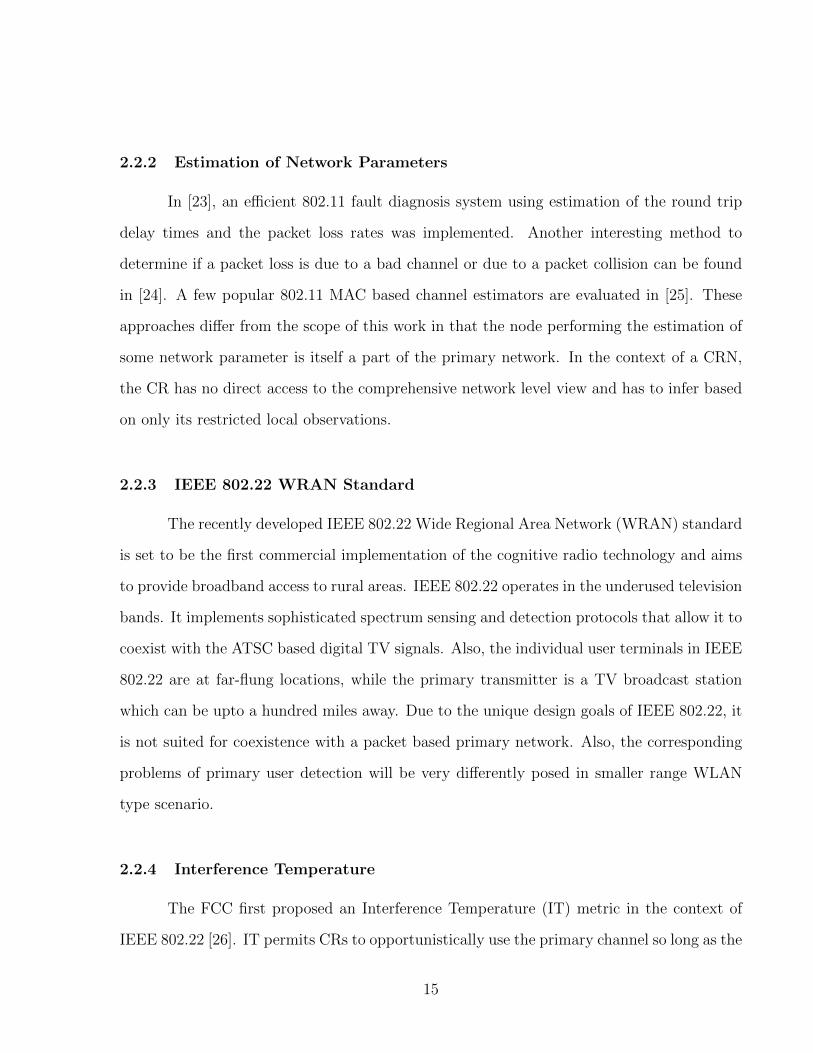
2.2.2 Estimation of Network Parameters
In [23], an efficient 802.11 fault diagnosis system using estimation of the round trip
delay times and the packet loss rates was implemented. Another interesting method to
determine if a packet loss is due to a bad channel or due to a packet collision can be found
in [24]. A few popular 802.11 MAC based channel estimators are evaluated in [25]. These
approaches differ from the scope of this work in that the node performing the estimation of
some network parameter is itself a part of the primary network. In the context of a CRN,
the CR has no direct access to the comprehensive network level view and has to infer based
on only its restricted local observations.
2.2.3 IEEE 802.22 WRAN Standard
The recently developed IEEE 802.22 Wide Regional Area Network (WRAN) standard
is set to be the first commercial implementation of the cognitive radio technology and aims
to provide broadband access to rural areas. IEEE 802.22 operates in the underused television
bands. It implements sophisticated spectrum sensing and detection protocols that allow it to
coexist with the ATSC based digital TV signals. Also, the individual user terminals in IEEE
802.22 are at far-flung locations, while the primary transmitter is a TV broadcast station
which can be upto a hundred miles away. Due to the unique design goals of IEEE 802.22, it
is not suited for coexistence with a packet based primary network. Also, the corresponding
problems of primary user detection will be very differently posed in smaller range WLAN
type scenario.
2.2.4 Interference Temperature
The FCC first proposed an Interference Temperature (IT) metric in the context of
IEEE 802.22 [26]. IT permits CRs to opportunistically use the primary channel so long as the
15

aggregate interference caused at the location of primary users does not exceed a predecided
threshold. The aggregate interference is quantified in terms of an IT similar to the noise
temperature concept. Figure 2.1 shows the potential new opportunities for spectrum access.
Thus, adoption of the IT metric opens up a whole new dimension in DSA methods and
unlocks previously unusable portions of the spectrum. IT based schemes are now an active
research area in cognitive radios and some promising recent developments based on IT can
be found in [27], [28], [29], [30]. Such an interference temperature formulation has many
theoretical and analytical advantages and holds great promise for implementation in future
CRNs. A possible practical obstacle towards implementing the Interference Temperature
Metric as envisaged by the FCC is that the IT limit is defined at the location of the primary
receiver. But the secondary transmitter has no effective way to measure the current IT at
the remote primary’s location. It can at most measure the interference temperature at its
own location and use it to approximate the IT at the primary receiver’s location.
2.2.5 SWIFT
Another related approach is SWIFT [31] in which the secondary user maintains a
wideband OFDM CR signal overlaid on an IEEE 802.11 signal by adding and deleting the
subcarriers so as to avoid using the subcarriers being used by the narrowband primary
network. Our work is different in a number of significant aspects. First, SWIFT is a white
space approach and aims to avoid the frequencies used by the PU by dynamically changing
SU occupied bins, whereas Protomac is a gray space approach and uses the Transmit Margin
(introduced in Section 2.4) to operate on the same bands as the PU by dynamically changing
SU transmit power and time. Second, SWIFT computes PU metrics but does not consider the
effect of these metrics on Quality of Service (QoS) of the PU. We can complete this link and
monitor the QoS because Protomac is based on the underlying stationarity of the PU network
and not limited to the instantaneous effect on PU. Since we monitor the longterm stationarity
16

Figure 2.1: FCC’s Interference Temperature Metric as proposed by the FCC
of the primary network Protomac is sensitive to effects that manifest after a significant
delay. For example, the decision to change the primary modulation scheme is a function of
the packet error rate averaged over the past few minutes. SWIFT cannot detect such macro
timescale effects which Protomac does. Third, SWIFT assumes a Gaussian distribution of all
PU metrics and based on this assumption it uses the Student’s t-test to only detect a change
in the mean of these statistics. But in reality, these statistics are strongly non-Gaussian, and
are usually multimodal whereas Protomac adopts nonparametric non-model-based methods
and can detect a change anywhere in the distribution. Our experimental results in Section
2.11.3 show that assuming a Gaussian distribution will be sub-optimal and leads to a severe
performance degradation since the distributions can change significantly in shape with only
a small change in their mean value. Finally the implementation of SWIFT only proposes
but does not actually implement the interarrival time and packet size statistics (see [31]
Sec 6). In this paper we present a unified treatment of our previous contributions [32–34]
and further significantly develop a holistic sensing and access system model with extensive
validation on a real world testbed.
17

Figure 2.2: Transmit Margin
18

2.3 Analysis of Network Traffic
The transmissions of the secondary user interfere with the primary network. While
designing the secondary system, the aim is to bound the maximum interference power re-
ceived by the primary users. Conventional Cognitive Radio systems use the sum interference
power received at the primary network as the design constraint as explained in Section 2.2.4.
This constraint is often formulated as an interference temperature. While mathematically
convenient, there are two inherent difficulties in implementing this interference constraint.
First the secondary user signal can be significantly attenuated when it reaches the primary
user. If we use the unattenuated signal to calculate the interference added, then we will be
wasting a lot of available capacity. Second, there is the problem of additivity where each
secondary user might individually ensure that it does not exceed the interference constraint
locally, but the sum interference due to all such secondary users as measured at the location
of the primary user might be much higher than the interference constraint. One possible
solution to these problems is to estimate the power spectral density at a remote location
as proposed in [35]. We will now introduce another alternate approach which is to modify
the level of abstraction from considering a single primary user and instead formulate the
problem as an effective interference limit for the entire primary network.
At any given instant the primary network is characterized by its Quality of Service
(QoS) metric. The QoS is measured via the available bandwidth, the latency and delay,
the throughput etc. At a coarser level, the QoS is captured by a variety of packet statistics
which can be calculated from the trace of the packets on the primary channel. Thus, if we
have time domain data of when each packet was sent, which primary node sent it to whom,
the data rate, SNR and duration of the packets, then we can completely characterize the
behavior and state of the primary network. Note that this also allows us to quantify the
behavior of the network at the remote node locations as described by their packet statistics.
For example, if a certain primary node experiences a higher interference than it can tolerate,
19

it will not be able to properly decode some of the packets sent to it. This will cause those
packets to be retransmitted and a resultant perturbation will be observed in the packet
statistics. While this is a special example, we can similarly argue that any perturbation in
the network behavior can be detectable after appropriate processing and thresholding. In
the next sections we will describe in detail the methods for doing precisely such network
state change detection.
2.4 Transmit Margin
We now proceed to motivate and define a Transmit Margin (TM) which is inspired by
the IT metric but circumvents the difficulty described above. Consider once more the scenario
depicted in Figure 2.2. Notice that the primary receiver requires a certain SNRmin =
PSignal,min
PNoise,maxto maintain its QoS. If the receiver noise level N0 is lower than PNoise,max or if
received signal power PSignal > PSignal,min then the channel can support additional secondary
power insertion equal to SNRactual − SNRmin without any effect on its Quality-of-Service
(QoS).
The IT concept was introduced with a goal of being able to safeguard the QoS experienced
by the primary network. This QoS is defined in terms of the network throughput, available
bandwidth, latency etc. Thus, the QoS depends on a host of factors each of which either
lies within the circle of influence of the Secondary Network or outside its circle of influence.
For example, an abrupt spike in primary traffic which leads to a increase in the packet
collision rate and decrease in QoS is not controllable by the Secondary Network. But, an
increased number of packet retransmissions caused by a rise in the Packet Error Rate (PER)
due to a degraded channel quality might be directly attributable to the secondary network’s
behavior. The Secondary transmission power acts as additive noise to the primary channel
and when increased beyond a threshold, it is capable of causing a drop in the primary QoS.
The Transmit Margin is defined as the allowable maximum secondary transmission power
20

which does not degrade the primary network QoS beyond a small tolerable predecided limit.
Thus Protomac retains the spirit of the IT concept, but shifts the test criteria from the PHY
layer (SNR) to the MAC layer (QoS). The degradation is measured with respect to the base
QoS which the Secondary Network observed before starting the transmission attempt. Also,
the TM as defined is highly conservative in that a degradation in primary QoS caused by
factors outside the secondary’s circle of influence will also be treated in the same way as one
caused by the secondary behavior, by a reduction of transmit power. The onus is always on
the secondary users to ensure that they do not interfere with the primary network. Also, the
change in QoS is tested through the network statistics which in turn are a direct indicator of
the channel quality as measured at the physical location of the primary system transceivers;
this implicitly allows Protomac to control the effect of the secondary network at the remote
primary locations. This is the cardinal advantage delivered by the use of a Transmit Margin.
2.5 Network-level Descriptors
Protomac observes the external behavior of the primary network to infer underlying
changes. In this section we describe the properties of the primary network that enable
Protomac to characterize it reliably. These properties rely on the probability distributions
of various observable quantities of the primary network. We will now describe the estimation
of the distributions of these primary network statistics.
The primary network observations are preprocessed in two stages. First, the samples
are randomized in a group-sequential manner, i.e., only a subset of the samples observed are
used. Specifically, every sample is accepted with a predecided probability γ. This sampling
scheme reduces the effects of the correlation between successive samples that arises due to
the implementation of the protocol, such as a packet transmission being always followed by
an acknowledgment after a fixed interval [18, 36]. The results here are obtained for typical
21

values of γ between 0.6 - 0.9. Second, the probability densities of the relevant statistics are
then estimated using kernel density estimation. The density has to be estimated such that
the distinct peaks in the density are not masked, while at the same time, it is smooth enough
to avoid spurious noise. The choice of the bandwidth h of the kernel used for this density
estimation has to be optimally set in order to achieve these goals and is calculated via the
procedure described in Section 2.8.9.
2.5.1 Primary Network can be characterized through its observable statistics
The SU node is not associated to the Primary Network and does not have direct access
to measure the Quality of Service parameters such as delay, bandwidth etc. Our algorithm
characterizes the instantaneous state of the primary network by tracking the metrics of the
primary network that the SU can observe. Specifically, the SU observes a) the primary
packet sizes that it can sense and b) the interarrival duration between consecutive primary
packets. These network statistics are summarized via building their probability distribution
functions. Although other network statistics can be incorporated into our algorithm, the
packet size and interarrival time distributions have the beneficial properties that they are
sensitive to the interference caused by the secondary users while being agnostic to the exact
implementation of the wireless protocol in the primary network.
2.5.2 Distribution of Statistics is relatively stationary over short time intervals
Through prolonged observation of the primary network statistic, it was observed that
the primary network state as described by the above network statistics varies slowly with
time. In other words, except for sudden disruptive events, the primary network demon-
strates short term time stationarity. This observation underlies and enables our proposed
algorithms. Empirically, this stationarity is prominently observed on a time scale of the in-
terval in which 50-200 packet arrivals per interval, i.e. 50/λ to 200/λ seconds, where λ is the
22

average arrival rate of packets on the primary channel. To quantify this time stationarity,
we calculated the KL divergence (see Section 2.8 for more details) between consecutive slots
and observed the number of consecutive slots over which the density of the network statistic
does not diverge significantly. Figure 2.3 shows that these statistics drift only slowly over
time, and that the rate of this drift depends on the traffic density of the primary network.
2.5.3 Changes in QoS of Primary Network are mirrored in its Network Statistics
The QoS is captured by a variety of packet statistics which can be calculated from
the trace of the packets on the primary channel. Thus, if we have time domain data of
when each packet was sent, which primary node sent it to whom, the data rate, SNR and
duration of the packets, then we can completely characterize the behavior and state of the
primary network. Note that this also allows us to quantify the behavior of the network
at the remote node locations as described by their packet statistics. For example, if a
certain primary node experiences a higher interference than it can tolerate, it will not be
able to properly decode some of the packets sent to it. This will cause those packets to be
retransmitted and a resultant perturbation will be observed in the packet statistics. While
this is a special example, we can similarly argue that any perturbation in the network
behavior can be detectable after appropriate processing and thresholding.Thus the QoS
of the Primary Network provides implicit feedback to the SU node about the interference
caused by its transmission at the remote location. We have validated this interlinking of PU
QoS and the observable PU statistics through a large number of experimental runs and a
representative result is shown in Figure 2.4. More results for a variety of operating conditions
are available on the authors’ website.
23

Figure 2.3: Decay of time stationarity over consecutive slots of 100 packet arrivals for a
threshold of 1.0
Figure 2.4: Dependence of Round-trip delay time and Network Statistics on Secondary
Interference
2.6 ProTOMAC: Description and Flowchart
In the previous section, we have presented the underlying principle that we can mon-
itor the effect of secondary system operation on the primary system’s Quality of Service via
a number of short term stationary network statistics. In this section, we will provide an
24
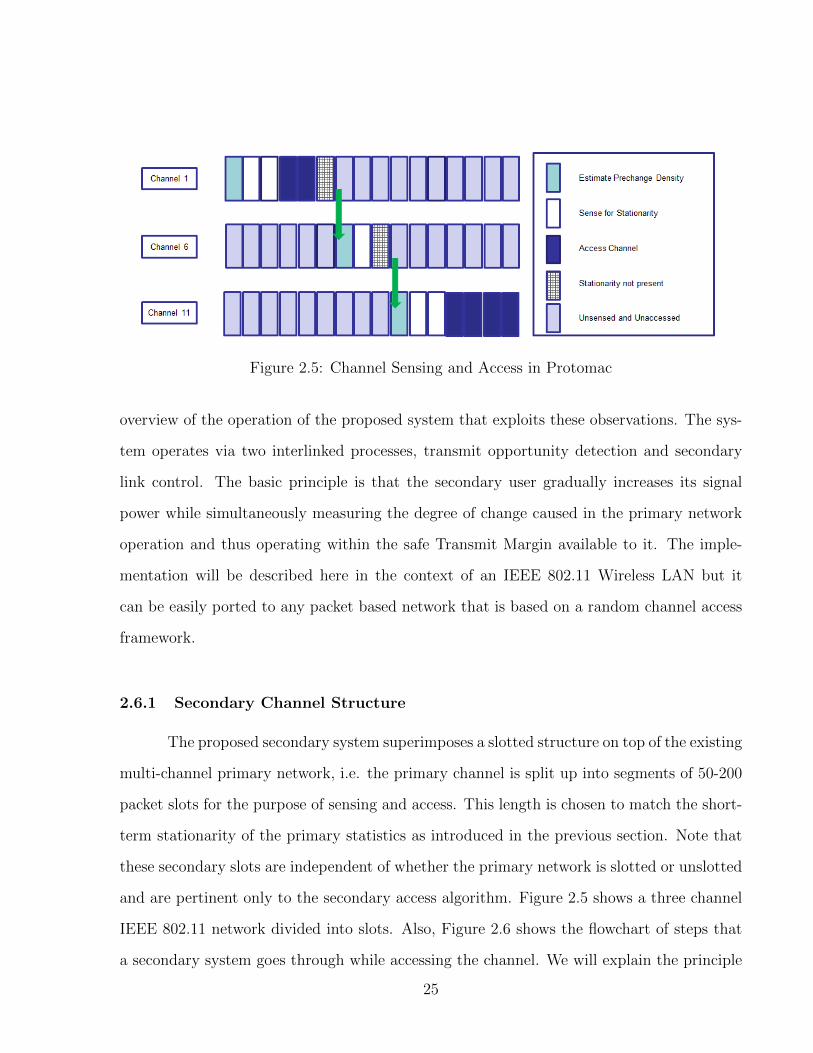
Figure 2.5: Channel Sensing and Access in Protomac
overview of the operation of the proposed system that exploits these observations. The sys-
tem operates via two interlinked processes, transmit opportunity detection and secondary
link control. The basic principle is that the secondary user gradually increases its signal
power while simultaneously measuring the degree of change caused in the primary network
operation and thus operating within the safe Transmit Margin available to it. The imple-
mentation will be described here in the context of an IEEE 802.11 Wireless LAN but it
can be easily ported to any packet based network that is based on a random channel access
framework.
2.6.1 Secondary Channel Structure
The proposed secondary system superimposes a slotted structure on top of the existing
multi-channel primary network, i.e. the primary channel is split up into segments of 50-200
packet slots for the purpose of sensing and access. This length is chosen to match the short-
term stationarity of the primary statistics as introduced in the previous section. Note that
these secondary slots are independent of whether the primary network is slotted or unslotted
and are pertinent only to the secondary access algorithm. Figure 2.5 shows a three channel
IEEE 802.11 network divided into slots. Also, Figure 2.6 shows the flowchart of steps that
a secondary system goes through while accessing the channel. We will explain the principle
25

steps that Protomac goes through during channel access.
2.6.1.1 Initialization
At initialization, every CR starts off with a sensing period when it observes the initial
state of the primary network without transmitting. During this period, the secondary net-
work calculates the traffic patterns and the rate at which the network statistics are changing
is estimated. This estimation of the transition probabilities and the short term stationarity
present in the primary network is used as a baseline to measure the effects on the QoS of
the primary users. Protomac proceeds to the next step only if the primary network displays
stationarity.
2.6.1.2 Channel Access
The Channel Access step is depicted in Figure 2.5. Once the primary network has
been deemed to be stationary, the secondary node uses the next slot to build an estimate of
the prechange distribution of the network statistics. The secondary node will now wait for
an additional Nsense slots. During these slots, the KL divergence of the network statistics is
calculated per slot, and only if the change is less than the preset threshold, it proceeds to the
next stage. The exact values of Nsense and the divergence threshold control the aggressiveness
of the system. After successfully waiting for Nsense slots, the cognitive radio is allowed to
start accessing the channel at a power level decided by the Transmit Power Control Loop.
2.6.1.3 Transmit Power Control Loop
Once the CR has determined that a transmit opportunity exists in the channel access
cycle, it proceeds to transmit its signal. This is done in a proactive manner, by increasing
the interference perceivable to the primary network. The allowable transmit power of each
26

CR is quantized into discrete levels as P1 = ∆P, P2 = 2∆P, ..., Pmax. The CR starts by
increasing its power to P1 and runs the change detection tests that will be described later. If
the test detects a change above the threshold, it ceases transmission immediately and during
the next access opportunity the transmit power is reduced to by one level while if the test is
negative, the transmit power is increased during the next access interval and the process is
repeated. After the secondary transmission is over, the channel transition probabilities are
updated.
2.6.1.4 Channel Hopping
If Protomac detects a change in the primary network, using the coarse change detec-
tion algorithms described in the next section, during any access slot, it immediately ceases
transmitting and does not continue to transmit for the remaining slot. It will restart sensing
the primary channel transition probabilities, and if these have been degraded, it will ran-
domly hop to one of the other primary channels and restart the Channel Access algorithm
in a similar manner to that currently implemented in the IEEE 802.22 standard.
2.7 Network Descriptors
The basic statistical principles underlying the methods proposed in this work can
be applied to any network statistic that remain relatively stationary over moderate time
periods. In this section, we motivate the adoption of the packet size and the retransmission
behavior of the network as suitable statistics for implementation using Protomac.
2.7.1 Packet Size
It is hypothesized that the primary network maintains a relatively constant packet
traffic rate, which is a reasonable assumption over a time window of a few minutes [37], [38].
27

Figure 2.6: Protomac Flowchart
This is reflected by the stationarity of the perceived available bandwidth over time intervals
on the order of minutes. The network traffic is succinctly characterized by the histogram
of the distribution of the packet sizes. The 802.11 protocol limits the maximum length of
the packets to 1548 bytes in practice. A high throughput traffic flow will have a histogram
concentrated more towards the higher packet sizes, while a low throughput traffic flow will
have a more evenly balanced histogram. The insertion of interference due to the secondary
transmitter will cause a shift in the histogram away from the one corresponding to high
traffic flow. The two principal reasons for this behavior are,
1. The secondary transmission acts as addition of noise to the channel and increases the
bit error rate (BER) for the primary packets. Also, the packet error rate (PER) is
proportional to the BER and the packet length. Thus, the bigger packets are more
prone to be received in error than the smaller packets.
2. The 802.11 MAC protocol has a fragmentation threshold which controls how longer
frames are fragmented into packets. This threshold changes dynamically and decreases
28

Figure 2.7: Experiment TestBed
29

when the node perceives an increased PER.
2.7.2 Packet Retry Rate
The 802.11 MAC retransmits a packet if the original transmission is unsuccessful. The
packet retry number flag is used to indicate such packets. The retransmissions might be due
to traffic congestion or an increased PER in the channel. It is possible to estimate the channel
quality from the proportion of packets that have this flag set and to assess the degradation
in primary QOS due to secondary user interference. A related alternate approach which
has been implemented by the authors tracks the primary channel quality through the lossy
intercepted data-ACK packet exchange as seen through secondary channels [39].
2.7.3 Channel Interarrival Time
The distribution of the interarrival period between successive packets on the wireless
channel is another statistic that will be used in this work. This statistic is interlinked to
the packet size statistic. As the channel quality degrades, the number of packet errors and
hence the number of packet retransmissions by the primary network increases. Also, this
in turn affects a number of other variables in the MAC schemes, such as Carrier Sense
Multiple Access in IEEE 802.11 WLANs, via the carrier sensing, random backoff periods,
retry attempts, and changes in modulation and coding type. Thus, a change in the Channel
Interarrival Time distribution is an indicator of these various underlying factors. In the rest
of the chapter we focus on the packet size statistic and the channel interarrival time statistic.
In the next section, we will cover the two methods that we will use to perform the
change detection in the network statistics, 1) Goodness-of-Fit tests and 2) Distributional
Divergence Measures.
30

2.8 Network Statistics Change Detection
In Section 2.5, it was shown that the distributions of the various network statistics
change slowly, except for a few abrupt shifts. These shifts are caused due to either secondary
transmitting above the Transmit Margin or due to other disturbances originating within the
primary network. The Protomac algorithm aims to detect the occurrence of this abrupt
change in the network statistics distribution. In this section, we will introduce the tech-
niques for detecting such an abrupt change in the primary network. The change detection
is implemented at two levels, coarse change detection and fine change detection. Coarse
change detection is used to simultaneously detect the change while the secondary user is
transmitting in its access slot. It must be able to detect the change very rapidly, and this
is achieved at the cost of an increase in the false alarm rate. We implement coarse change
detection using a modified Goodness-of-Fit test and a group sequential Kullback-Leibler di-
vergence update method. On the other hand, the fine change detection technique is used
to decide, with high confidence and low false alarms, whether the network statistics distri-
bution has changed after the secondary user finishes its transmission in that slot. We use
the Kullback-Leibler (KL) divergence between the old and new distributions as the baseline
to decide whether a change has occurred. We will now cover these coarse and fine change
detection techniques in more detail and briefly introduce the concept of Goodness-of-Fit
testing. We will develop two novel GoF tests, the sequential Kolmogorov-Smirnov test and
the Parallelized Goodness-of-Fit test, and derive a fast group-sequential method to update
the KL divergence.
2.8.1 Goodness-of-Fit Tests
Goodness-of-fit (GOF) tests are used to check whether the samples are from a given
probability distribution [40–42]. Consider a random sample of n independent and identically
distributed observations x1 < x2 < x3 < ... < xn arranged in ascending order. The Goodness
31

of Fit (GoF) test is a one sided hypothesis test for H0 that this sample was drawn from a
distribution with a Cumulative Distribution Function (CDF) F0. The hypothesis to be tested
are formulated as shown.
H0 : F (x) = F0(x) for all values of x, (2.1)
H1 : F (x) 6= F0(x) for at least one value of x, (2.2)
where F (x) is the empirical CDF of the sample. Thus, these tests are ideal for testing
for deviations from the prechange network statistics distribution. In this work we have
implemented a novel suite of multi-chart multi-type GoF tests. There are two families of
Goodness of Fit tests: 1) Kolmogorov Smirnov Type tests which use the L1 norm and 2)
The Cramer von-Mises type tests which use the L2 norm. The KS test has the following
desirable properties:
1. The KS test is preferable if the sample size is small, as the KS statistic is exact even
in that case [42]. This proves valuable in formulating a sequential version of the test.
2. The KS test is the only non-parametric goodness-of-fit test with exactly derivable
confidence bands [43].
3. The KS statistic is a distribution-free statistic.
2.8.2 Implementation of the Kolmogorov-Smirnov test
Let X1, X2, ..., Xn be a random sample of size n drawn from an unknown distribution
F(x). We want to test the hypothesis that F (x) = F0(x). First, the empirical cumulative
distribution function (e.d.f) of the n samples is calculated as Sn(x).
Sn(x) =Number of sample observations ≤ x
n(2.3)
32

Now, we evaluate the KS distance between the prechange cumulative distribution F0(x) and
the empirical cumulative distribution Sn(x). When plotted graphically, this gives us the
greatest vertical distance between the two distributions and is defined as the KS distance
Dn,
Dn = supx|F0(x)− Sn(x)|. (2.4)
We can also define two additional metrics for a one-sided KS test. D+n and D−n are used to
formulate one-sided confidence bands for finer testing.
D+n = sup
x[F0(x)− Sn(x)] (2.5)
D−n = supx
[Sn(x)− F0(x)] (2.6)
The distribution-free property of the KS test means that the KS statistics D, D+, and D−
have a distribution function that is independent of the exact form of F0(x). In his classic
paper, Kolmogorov has proved the existence of a limiting value of Dn [44]. Also, there are
formulas which let us calculate the statistic for small finite n and asymptotic approximations
as n→∞, e.g,
limn→∞
Pr(√nDn ≤ d) =
∞∑j=−∞
(−1)je−2j2d2 . (2.7)
The Glivenko-Cantelli theorem [45] states that when F = F0, the KS statistic Dn vanishes
as shown,
Pr(
limn→∞
Dn = 0)
= 1. (2.8)
As a result, we can be confident that our test will be strongly consistent against all alterna-
tives and the false hypothesis will be rejected with probability one as we accumulate more
and more samples, i.e, as n→∞.
Let α be the significance level corresponding to the 100(1 − α) confidence interval.
Also, parameter dn(α) is the critical value for a given α, i.e, it is the probability of incorrectly
33

rejecting the hypothesis in equation (3.3). We can find the corresponding critical region of
the test as shown in (2.9),
PDn ≥ dn(α) = α. (2.9)
Massey gives recursive expressions and tables to calculate the critical value for a given α [46].
Note that α is an indicator of the probability of misdetection of the test, which we investigate
in section 2.11.
A confidence band [42] [47] is an alternate way of looking at the problem of testing
for goodness-of-fit. We will reverse the traditional use of the confidence band wherein we
find the 1 − α quantile corresponding to dα of the KS statistic and threshold Dn against
the dα distance. Instead, we will use dα to set a confidence band for the whole postchange
density function. Thus, regardless of the exact form of the prechange density, we get the
two equivalent statements in equations (2.10) and (2.12). Equation (2.12) states that the
prechange density function F0(x) lies entirely within a band of ±dα from the empirical
distribution function Sn(x) with a probability of 1− α.
PDn = supx|Sn(x)− F0(x)| ≥ dα = α (2.10)
PSn(x)− dα ≤ F0(x) ≤ Sn(x) + dα = 1− α for ∀x (2.11)
PF0(x)− dα ≤ Sn(x) ≤ F0(x) + dα = 1− α for ∀x (2.12)
2.8.3 Sequential Kolmogorov-Smirnov Test
We implement a novel modification of the KS test in Protomac. In section 2.8.2, we
have reviewed how to setup a KS test. Here, we propose a sequential version of the KS test.
According to the authors’ best knowledge, there has been only one previous formulation of
a sequential version of the KS test by Hawkins [48]. But, the Hawkins approach proposed
a sequential version to tackle the problem of quickest change detection, i.e, the aim was to
34

estimate the change point of a given time series, not the magnitude of the change. This
makes the Hawkins approach unsuitable for the situation under consideration here. We
present a novel formulation which works by iteratively estimating the KS statistics in an
online manner.
It is important to be able to reach a decision in favor of a hypothesis in a timely and
reliable manner. A sequential formulation of the KS test will minimize the time required to
reach the decision. In equation (2.4), it is seen that the KS statistic depends on the number
of samples n. This dependence implies that as the number of samples increases, the width of
the confidence band of the test cumulative distribution decreases. We explain the operation
of the sequential test with help of figure.2.8 which shows the plot of two possible drifts in
test statistic Dn with increasing n. Also, superimposed on the plot are the dn(α) contours
corresponding to increasing values of α. A significance level for the test, αth, is initialized
to a predecided value. The test begins by collecting samples and updating the empirical
cumulative distribution function at each step.
In Protomac, the KS test is evaluated in a group-sequential manner for rapid change
detection, i.e, in any secondary slot where the SU starts transmitting, it also simultaneously
begins to collect samples of primary network statistics to run the test. Starting at 10 samples,
the KS statistic is reevaluated after collecting every additional 5 samples. This ensures that
if the underlying distribution has undergone a significant change, we can detect it in a faster
time, and immediately cease secondary transmission to minimize the effect on the PU. But
most goodness-of fit tests have a high variance of the statistic at small sample sizes (≤ 30
samples) and this leads to a very high false alarm rate and the rejection of a large proportion
of valid transmit opportunities. The KS statistic exhibits a low sensitivity at these small
sample sizes and this sensitivity rapidly improves as the sample size increases above 20. We
exploit this behavior through a sequential shrinkage of test significance. At every step in
the group sequential process, the significance level of the KS test is decreased in line with
35

Figure 2.8: Sequential KS Test
the increase in the performance of the KS statistic, i.e., the corresponding confidence band
of the KS test centered around the null distribution increases. The implementation details
and results for this sequential KS test are given in Section 2.11.
2.8.4 Cramer von-Mises GoF Test
The Cramer von-Mises statistic ω2n is defined in (2.13) and is the integrated squared
difference between the original distribution and the empirical distribution [49].
ω2n = n
∫ ∞−∞
(Fn(x)− F0(x))2 dF0(x). (2.13)
Substituting ti = F0(xi), we have,
ω2n = n
∫ 1
0
(Fn(t)− t)2 dt, (2.14)
36

Figure 2.9: Ψ(t) for various GoF tests
where the ti are Uniform (0,1) random variables. After some manipulation, we obtain the
easily computable form as shown in (2.15).
ω2n = n
n∑k=1
(tk −
k − 1/2
n
2
+1
12n
). (2.15)
The Cramer von Mises test is sensitive to deviations in the central region of the dis-
tribution function whereas the related Anderson-Darling test is sensitive to the deviations
in the upper and lower tails of the distribution and the Viollaz-Rodriguez test can be cus-
tomized to be sensitive to either the upper tail or the lower tail deviations. Our method
forms a suite of these GoF tests as explained in the next section.
37
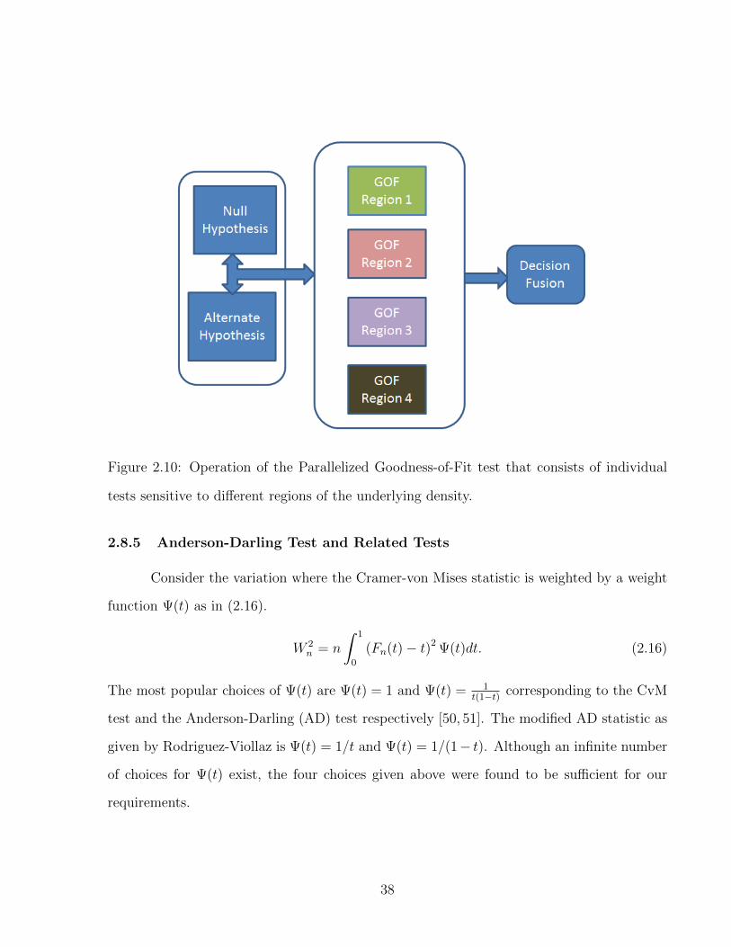
Figure 2.10: Operation of the Parallelized Goodness-of-Fit test that consists of individual
tests sensitive to different regions of the underlying density.
2.8.5 Anderson-Darling Test and Related Tests
Consider the variation where the Cramer-von Mises statistic is weighted by a weight
function Ψ(t) as in (2.16).
W 2n = n
∫ 1
0
(Fn(t)− t)2 Ψ(t)dt. (2.16)
The most popular choices of Ψ(t) are Ψ(t) = 1 and Ψ(t) = 1t(1−t) corresponding to the CvM
test and the Anderson-Darling (AD) test respectively [50, 51]. The modified AD statistic as
given by Rodriguez-Viollaz is Ψ(t) = 1/t and Ψ(t) = 1/(1− t). Although an infinite number
of choices for Ψ(t) exist, the four choices given above were found to be sufficient for our
requirements.
38

2.8.6 The Parallelized GoF Test
The GoF statistics above form the Generalized Cramer-von Mises family where the
weight function Ψ(t) lets us factor in the region where the deviation is most likely to occur.
The Cramer-von Mises test is sensitive to deviations in the central region of the distribution
function whereas the related Anderson-Darling test is sensitive to the deviations in the upper
and lower tails of the distribution and the Viollaz-Rodriguez test can be customized to be
sensitive to either the upper tail or the lower tail deviations. Depending on the application,
statisticians recommend one of these tests to maximize the test power under the alternative
hypothesis H1. In our case, the alternate distributions are different in shape depending on
the exact change caused in the Primary network and on the traffic characteristics which
cannot be predicted in advance while formulating the test.
In order to solve this problem of complete lack of a priori knowledge regarding which
test will have the highest power, we propose to apply a suite of these GoF tests at the same
time. Such a parallelized Goodness-of-Fit test is implemented by performing the Cramer-
von Mises test, the Anderson-Darling test and the its two Sinclair-Rodriguez-Viollaz variants
simultaneously. The final decision is made via ORing the individual decisions. This has the
effect of formulating the parallelized test in a conservative manner and is desirable since
cognitive radio networks implement the philosophy that it is critical to robustly detect any
possibility of interference with the primary network. The parallelized Goodness-of-Fit test as
implemented in Figure 2.10 is highly sensitive across the whole support of the packet statistic
distribution since each constituent GoF test is sensitive to a change in certain specific regions
of the underlying density of the packet statistics. The performance of this test is described
in Section 2.11.
39

2.8.7 Kullback-Leibler Divergence
Protomac uses fine change detection based on the Kullback-Leibler measure to decide
at the end of secondary slot if the primary network statistics have changed. Due to the
interference introduced by the secondary users, the initially estimated prechange density
changes by an unknown degree to the new postchange density. In this section we will examine
ways to measure the degree of this change using the concepts of information theory [52].
There are several ways to measure the unlikeness of two distributions such as Kullback Leibler
divergence measures and Chernoff Distance measures. All the divergence measures we cover
below are members of a generalized class of information theoretic divergence measures called
Ali-Silvey distances but each measure is suited for particular class of applications due to its
unique properties [53].
The Kullback-Leibler (KL) divergence was introduced by Kullback in the context of
statistical inference [54]. Let F1 and F2 be two probability distributions and let f1(x) and
f2(x) be the corresponding probability density functions. The KL divergence from F1 to F2
is defined as,
D(F1 ‖ F2) =
∫f1(x)log
(f1(x)
f2(x)
)dx. (2.17)
Equation (2.17) shows that the KL divergence is also the expected value of the log-
likelihood ratio of the two densities under consideration, where Λ(x) = f1(x)f2(x)
. The expectation
is taken with respect to F1 to get D(F1 ‖ F2) as shown,
D(F1 ‖ F2) = EF1 [logΛ(x)]. (2.18)
Although the KL divergence will be used as a distance measure, note that while the
KL divergence follows the additive property, it does not satisfy the triangle inequality nor is
it a symmetric measure, i.e,
D(F1 ‖ F2) 6= D(F2 ‖ F1). (2.19)
40

But, the KL divergence is always non-negative and equals zero if and only if the two distri-
butions are equal. Thus we can justifiably use the KL divergence to measure the similarity
between two probability distributions, i.e, D(F1 ‖ F2) ≥ 0 and
D(F1 ‖ F2) = 0 ⇐⇒ F1 = F2. (2.20)
A symmetric version of the KL divergence was defined by Jeffreys as in equation (2.21) and
is called the J-divergence [55].
J(F1 ‖ F2) = D(F1 ‖ F2) +D(F2 ‖ F1). (2.21)
For our application, we are interested only in a measure of the distributional difference after
we introduce the interference. These measures will be taken for each transmit power level.
Thus, we can expect that the asymmetric KL divergence should be sufficient for our needs.
Indeed, the experiments demonstrate the superior performance of the KL divergence as
compared to the J-divergence. The reason for this is that the prechange density is accurate
while the postchange density is only approximate and hence EFPre[logΛ(x)] is better than
EFPost[logΛ(x)]. The KL divergence of discrete distributions with a probability mass function
is calculated as shown,
D(F1 ‖ F2) =N∑x=1
f1(x) log
(f1(x)
f2(x)
). (2.22)
2.8.8 Bhattacharyya Distance
The Chernoff distance between distributions F1 and F2 is C(F1 ‖ F2) = −log(µ(t)),
where µ(t) is defined in (2.23) [56].
µ(t) =
∫[f1(x)]1−t[f2(x)]t dx. (2.23)
The Chernoff class of distance measures includes a wide subset of divergences. But their
evaluation involves solving a difficult optimization problem [57]. The Bhattacharyya distance
41
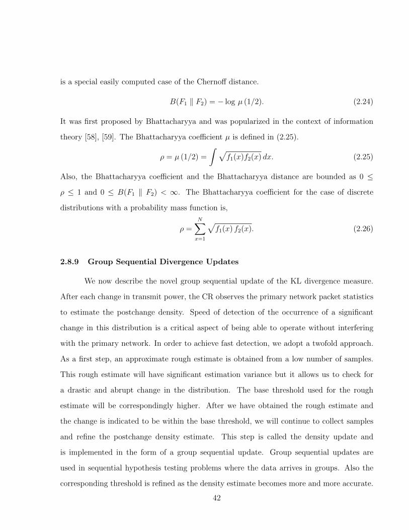
is a special easily computed case of the Chernoff distance.
B(F1 ‖ F2) = − log µ (1/2). (2.24)
It was first proposed by Bhattacharyya and was popularized in the context of information
theory [58], [59]. The Bhattacharyya coefficient µ is defined in (2.25).
ρ = µ (1/2) =
∫ √f1(x)f2(x) dx. (2.25)
Also, the Bhattacharyya coefficient and the Bhattacharyya distance are bounded as 0 ≤
ρ ≤ 1 and 0 ≤ B(F1 ‖ F2) < ∞. The Bhattacharyya coefficient for the case of discrete
distributions with a probability mass function is,
ρ =N∑x=1
√f1(x) f2(x). (2.26)
2.8.9 Group Sequential Divergence Updates
We now describe the novel group sequential update of the KL divergence measure.
After each change in transmit power, the CR observes the primary network packet statistics
to estimate the postchange density. Speed of detection of the occurrence of a significant
change in this distribution is a critical aspect of being able to operate without interfering
with the primary network. In order to achieve fast detection, we adopt a twofold approach.
As a first step, an approximate rough estimate is obtained from a low number of samples.
This rough estimate will have significant estimation variance but it allows us to check for
a drastic and abrupt change in the distribution. The base threshold used for the rough
estimate will be correspondingly higher. After we have obtained the rough estimate and
the change is indicated to be within the base threshold, we will continue to collect samples
and refine the postchange density estimate. This step is called the density update and
is implemented in the form of a group sequential update. Group sequential updates are
used in sequential hypothesis testing problems where the data arrives in groups. Also the
corresponding threshold is refined as the density estimate becomes more and more accurate.
42
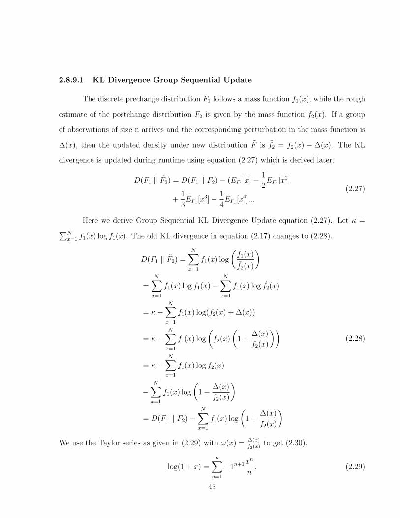
2.8.9.1 KL Divergence Group Sequential Update
The discrete prechange distribution F1 follows a mass function f1(x), while the rough
estimate of the postchange distribution F2 is given by the mass function f2(x). If a group
of observations of size n arrives and the corresponding perturbation in the mass function is
∆(x), then the updated density under new distribution F is f2 = f2(x) + ∆(x). The KL
divergence is updated during runtime using equation (2.27) which is derived later.
D(F1 ‖ F2) = D(F1 ‖ F2)− (EF1 [x]− 1
2EF1 [x
2]
+1
3EF1 [x
3]− 1
4EF1 [x
4]...
(2.27)
Here we derive Group Sequential KL Divergence Update equation (2.27). Let κ =∑Nx=1 f1(x) log f1(x). The old KL divergence in equation (2.17) changes to (2.28).
D(F1 ‖ F2) =N∑x=1
f1(x) log
(f1(x)
f2(x)
)
=N∑x=1
f1(x) log f1(x)−N∑x=1
f1(x) log f2(x)
= κ−N∑x=1
f1(x) log(f2(x) + ∆(x))
= κ−N∑x=1
f1(x) log
(f2(x)
(1 +
∆(x)
f2(x)
))
= κ−N∑x=1
f1(x) log f2(x)
−N∑x=1
f1(x) log
(1 +
∆(x)
f2(x)
)
= D(F1 ‖ F2)−N∑x=1
f1(x) log
(1 +
∆(x)
f2(x)
)
(2.28)
We use the Taylor series as given in (2.29) with ω(x) = ∆(x)f2(x)
to get (2.30).
log(1 + x) =∞∑n=1
−1n+1xn
n. (2.29)
43
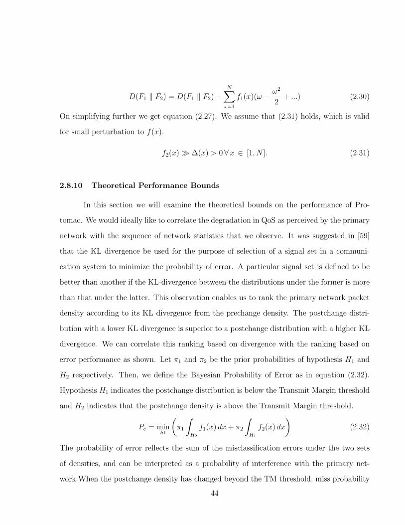
D(F1 ‖ F2) = D(F1 ‖ F2)−N∑x=1
f1(x)(ω − ω2
2+ ...) (2.30)
On simplifying further we get equation (2.27). We assume that (2.31) holds, which is valid
for small perturbation to f(x).
f2(x) ∆(x) > 0 ∀x ∈ [1, N ]. (2.31)
2.8.10 Theoretical Performance Bounds
In this section we will examine the theoretical bounds on the performance of Pro-
tomac. We would ideally like to correlate the degradation in QoS as perceived by the primary
network with the sequence of network statistics that we observe. It was suggested in [59]
that the KL divergence be used for the purpose of selection of a signal set in a communi-
cation system to minimize the probability of error. A particular signal set is defined to be
better than another if the KL-divergence between the distributions under the former is more
than that under the latter. This observation enables us to rank the primary network packet
density according to its KL divergence from the prechange density. The postchange distri-
bution with a lower KL divergence is superior to a postchange distribution with a higher KL
divergence. We can correlate this ranking based on divergence with the ranking based on
error performance as shown. Let π1 and π2 be the prior probabilities of hypothesis H1 and
H2 respectively. Then, we define the Bayesian Probability of Error as in equation (2.32).
Hypothesis H1 indicates the postchange distribution is below the Transmit Margin threshold
and H2 indicates that the postchange density is above the Transmit Margin threshold.
Pe = minh1
(π1
∫H2
f1(x) dx+ π2
∫H1
f2(x) dx
)(2.32)
The probability of error reflects the sum of the misclassification errors under the two sets
of densities, and can be interpreted as a probability of interference with the primary net-
work.When the postchange density has changed beyond the TM threshold, miss probability
44
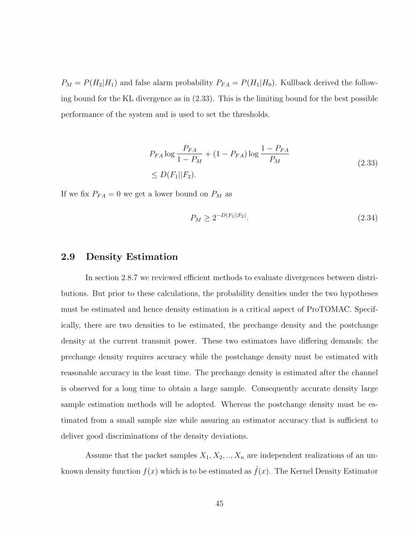
PM = P (H2|H1) and false alarm probability PFA = P (H1|H0). Kullback derived the follow-
ing bound for the KL divergence as in (2.33). This is the limiting bound for the best possible
performance of the system and is used to set the thresholds.
PFA logPFA
1− PM+ (1− PFA) log
1− PFAPM
≤ D(F1||F2).
(2.33)
If we fix PFA = 0 we get a lower bound on PM as
PM ≥ 2−D(F1||F2). (2.34)
2.9 Density Estimation
In section 2.8.7 we reviewed efficient methods to evaluate divergences between distri-
butions. But prior to these calculations, the probability densities under the two hypotheses
must be estimated and hence density estimation is a critical aspect of ProTOMAC. Specif-
ically, there are two densities to be estimated, the prechange density and the postchange
density at the current transmit power. These two estimators have differing demands; the
prechange density requires accuracy while the postchange density must be estimated with
reasonable accuracy in the least time. The prechange density is estimated after the channel
is observed for a long time to obtain a large sample. Consequently accurate density large
sample estimation methods will be adopted. Whereas the postchange density must be es-
timated from a small sample size while assuring an estimator accuracy that is sufficient to
deliver good discriminations of the density deviations.
Assume that the packet samples X1, X2, .., Xn are independent realizations of an un-
known density function f(x) which is to be estimated as f(x). The Kernel Density Estimator
45

400 600 800 1000 1200 1400 16000
1
2
3
4
5
6
7x 10
−3
Packet Length
Kernel Density Estimates
P
Tx = 0
PTx
= 200
PTx
= 400
PTx
= 600
PTx
= 800
PTx
= 1000
PTx
= 1400
Figure 2.11: KDEs of CAP1 Dataset for increasing Tx Power with full capture duration
46

(KDE) is given as
fh(x) =1
n
n∑i=1
Kh(x−Xi), (2.35)
where the kernel function Kh is defined as,
Kh(u) =1
hK(uh
). (2.36)
Appropriate choice of the kernel function Kh and an optimal selection of the smoothing
factor or bandwidth h are the two critical aspects of KDE. The accuracy of the estimated
density function is quantified by the Asymptotic Mean Square Integrated Error(AIMSE)
criteria defined as
AIMSE(h) =1
nhR(K) + h4
(µk(K)
4
)2
R(f”), (2.37)
where the functional µk(K) =∫xkK(x)dx and R(K) =
∫K2(x)dx. The first term in
equation (2.37) is the asymptotic integrated variance and the second term is the asymptotic
integrated bias. Minimization of the AIMSE gives the optimal bandwidth.
2.9.1 Deheuvel’s Rule of Thumb Method
The optimal value of h is obtained by solving equation (2.37) as
h∞ =
(R(k)
µ22(K)R(f ′′)
) 15
n−15 (2.38)
But R(f ′′) is an unknown since f itself is the density to be estimated. We get around this
difficulty by using the Deheuvel’s Rule of Thumb method [60]. It involves approximating f
through another reference density function which is rescaled to have a variance equal to the
sample variance. Using a standard Gaussian as the reference distribution, the bandwidth is
estimated as,
ˆhrot = 1.06σn−15 (2.39)
where σ is the sample variance.
47
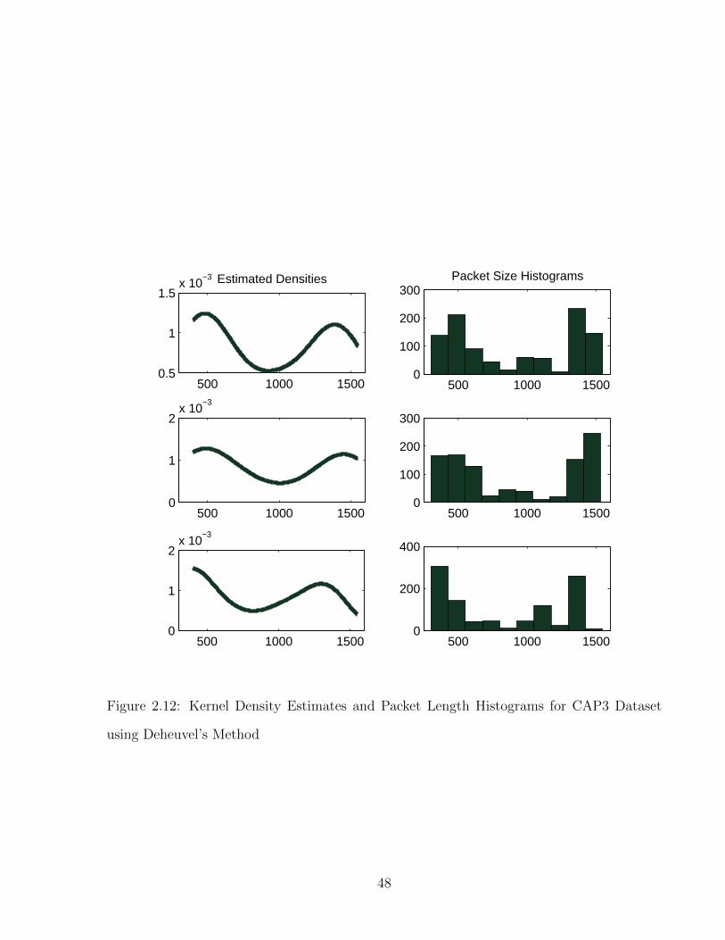
500 1000 15000.5
1
1.5x 10
−3 Estimated Densities
500 1000 15000
100
200
300Packet Size Histograms
500 1000 15000
1
2x 10
−3
500 1000 15000
100
200
300
500 1000 15000
1
2x 10
−3
500 1000 15000
200
400
Figure 2.12: Kernel Density Estimates and Packet Length Histograms for CAP3 Dataset
using Deheuvel’s Method
48

0 500 1000 1500 20000
0.5
1
1.5
2
2.5x 10
−3
Packet Length
Den
sity
Estimated Densities
0 500 1000 1500 20000
0.005
0.01
0.015
0.02
0.025
0.03
Packet Length
Den
sity
Estimated Densities
0 500 1000 1500 20000
0.005
0.01
0.015
0.02
Packet Length
Den
sity
Estimated Densities
0 500 1000 1500 20000
0.5
1
1.5
2
2.5
3x 10
−3
Packet Length
Den
sity
Estimated Densities
0 500 1000 1500 20000
0.005
0.01
0.015
0.02
0.025
Packet Length
Den
sity
Estimated Densities
0 500 1000 1500 20000
0.005
0.01
0.015
0.02
0.025
Packet Length
Den
sity
Estimated Densities
Figure 2.13: Demonstration of Time Stationarity over Captures for 6 increasing Transmission
Power Levels
2.10 Experimental Testbed Setup
In this section we describe the experimental testbed based implementation of Pro-
TOMAC. Figure 2.7 shows the setup of the testbed. The interactions between the primary
and secondary networks are illustrated in the figure. The CRN consists of colocated Wireless
Sniffers and Software Radios acting together as the secondary nodes. The primary network
is an IEEE 802.11g WLAN network.
2.10.1 Primary Network Configuration
IEEE 802.11 channels lie within the license free Industrial, Scientific and Medical
(ISM) band. Also, IEEE 802.11 shares the ISM band with a variety of legacy devices like
microwave ovens, Bluetooth and cordless phones. These legacy devices are sources of inter-
ference and a host of methods have been developed to avoid or to minimize this interference.
49

Newer technologies like Bluetooth have complex MAC protocols to allow coexistence with
802.11 [61]. These interference mitigation methods have been designed on a case-by-case
ad-hoc basis. The advent of dynamic spectrum use demands generalized non-interfering
spectrum access methods. ProTOMAC provides an open-ended and flexible framework for
an intelligent radio access mechanism within the philosophy of CRNs.
The testbed has been setup in the laboratory and is co-located with the University’s IEEE
802.11g WLAN. The 802.11g network is configured in the Infrastructure mode in which the
individual 802.11g basestations (BS) connect to a central Access Point (AP) and form a
cell. The presence of multiple overlapping cells creates a dense grid where nodes have the
choice to switch to alternate channels or to change association to an adjoining cell. For
example, Capture Set 1 consists of data transfer between 28 nodes and 6 APs. Analytical
modeling of such an extensive setup is not easily achieved. Instead, we have implemented
an empirical approach which dynamically tracks the statistical behavior of the network in a
non-parametric non model-based manner as explained in detail in section 2.6. As the sec-
ondary node transmits at a low power, the maximum probability of interference is presented
to the 802.11 nodes directly within the range of the secondary network.
2.10.2 Secondary Network Configuration
The secondary network consists of two Software Defined Radios (SDR). Each SDR
is composed of an Universal Software Radio Peripheral (USRP) manufactured by Ettus
Research which has a USB 2.0 based link to a laptop computer [62]. The USRPs are equipped
with a RF front-end board RFX2400 capable of simultaneously transmitting and receiving.
The RFX2400 has a frequency range of 2.3 to 2.9 GHz and has been designed to operate in
the ISM band (2.4 to 2.486 GHz). The USRP is programmed and controlled via the GNU
Radio suite of open source software radio and signal processing packages [63]. Also, a 2.4
GHz Intel Core2 Duo machine running the Ubuntu 8 Heron operating system interfaces with
50
the USRPs.
SDR 1 is configured as the transmitter and broadcasts at 2.412 GHz which is the center
frequency of channel 1 in IEEE 802.11. The transmission power is a dynamically controlled
variable. RFX2400 based USRPs have a maximum transmit power of 50 mW (17 dBm). SDR
2 is configured as the receiver and positioned at a distance of 1 m to 5 m. Throughout the
series of experiments, SDR 2 was able to receive and demodulate the transmitted sequence
succesfully. Section 2.12.4 gives details of the secondary link performance. An Intel Wireless
4965 Network Adapter card controlled via the Kismet Wireless Sniffer captured and logged
the 802.11 network traffic. The sniffers were colocated with the secondary transmitter and
receiver.
2.10.3 Implementation Issues
We demonstrate the performance of ProTOMAC with the help of three representative
runs, the outcomes of which are recorded in primary network packet captures labeled CAP1,
CAP2 and CAP3. Here we will describe the results in detail using CAP1 with brief comments
on the other runs. The three ProTOMAC runs occurred at different times of the day and
encountered varied network traffic. Thus, taken together we establish the robustness of
ProTOMAC under the gamut of situations that might be encountered in practice. The
distribution of the packet sizes and interarrival times was used as the network statistic as in
Section 2.3.
2.10.3.1 Study of Network Stationarity
The short term stationarity of the primary network can be shown through a rep-
resentative example where we observed the IEEE 802.11 network at three different traffic
conditions, busy traffic, medium traffic and low traffic. For each case the density of the
51

packet interarrival times on the primary network was calculated for consecutive slots where
each slot consisted of 100 packet arrivals. Then the KL divergence of each slot was found with
respect to slots observed at increasing delays and finally the network statistic was deemed
to have changed if the calculated KL divergence was higher than a threshold, which was 1.0
in this case. The probability that the network statistic changes over time is then plotted in
Figure 2.3. It can be seen that for the low traffic network, there is a 70 % probability that
the network statistics are unchanged after 4 consecutive slots, while this probability is still
more than 50 % when observed over a 6 slot interval. In other experiments, a stationarity
probability of 50-90 % was observed over a 6 slot interval. The exact degree of stationarity
changes with every network state and observation time. Protomac works by quantifying this
stationarity by the probability of change over consecutive slots, and then by continuously
monitoring this transition probability. Protomac stops using the channel and seek another
channel if there is a 10 percentage point fall in the underlying network stationarity.
2.11 Experimental Results For Goodness of Fit Tests
2.11.1 Sequential Kolmogorov-Smirnov Test
The method presented in the previous sections was implemented on three datasets of
packet captures. Here will explain the results for a representative case of Dataset 2. The
secondary transmission power was increased uniformly from zero upto 7 mW in three steps as
2.3mW, 4.6mW and 7mW . Figure 2.14 shows the histograms of the packet sizes for the four
transmission power levels. This power was sufficient to cause an inoperable interference to
primary base stations within a 1.2 m radius of the secondary transmitter, while the primary
base station was tested to work properly at a range of 2.5 m from the secondary transmitter.
Also, a secondary receiver could decode the transmissions at 2.3 mW at a distance of upto
12 m to set up a working secondary link. The data rate of the primary network dropped
52
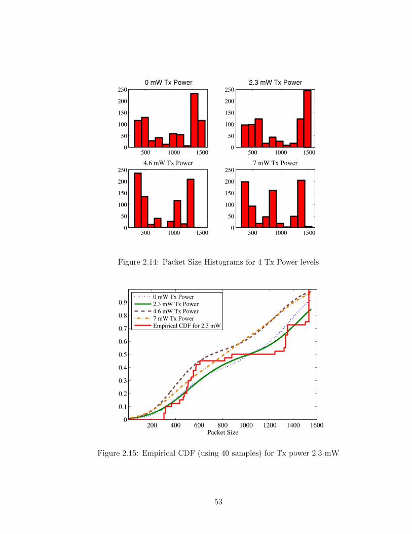
500 1000 15000
50
100
150
200
250
4.6 mW Tx Power
500 1000 15000
50
100
150
200
250
7 mW Tx Power
500 1000 15000
50
100
150
200
250
2.3 mW Tx Power
500 1000 15000
50
100
150
200
250
0 mW Tx Power
Figure 2.14: Packet Size Histograms for 4 Tx Power levels
200 400 600 800 1000 1200 1400 16000
0.1
0.2
0.3
0.4
0.5
0.6
0.7
0.8
0.9
Packet Size
0 mW Tx Power
2.3 mW Tx Power
4.6 mW Tx Power
7 mW Tx Power
Empirical CDF for 2.3 mW
Figure 2.15: Empirical CDF (using 40 samples) for Tx power 2.3 mW
53

0 200 400 600 800 1000 1200 1400 16000
0.1
0.2
0.3
0.4
0.5
0.6
0.7
0.8
0.9
1
Packet Size
0 mW Tx Power
2.3 mW Tx Power
4.6 mW Tx Power
7 mWTx Power
Empirical CDF for 4.6 mW
Figure 2.16: Empirical CDF (using 40 samples) for Tx power 4.6 mW
marginally from an initial 0.161 Mbps to 0.156 Mbps for a transmit power of 2.3 mW and to
0.121 Mbps for a transmit power of 4.6 mW. The Adaptive Modulation and Coding (AMC)
mode of the primary WLAN was unchanged for all 4 secondary transmit power levels but
changed if we attempted to increase the power further. Application of our method allowed a
Tx power of 2.3 mW but curtailed the secondary from transmitting at 4.6 mW or at 7 mW.
Thus, we were able to safely and reliably create a transmission opportunity and setup an
operational secondary link with only a marginal effect on the QOS of the primary network.
Similar results and threshold transmit powers were obtained for the other datasets.
Figure 2.15 shows the kernel density estimates of the packet captures. The densities were
estimated using the full duration of the captures and are considered to be the baseline
accurate estimate of the CDFs. Note the slight shift in the CDF curve when secondary
power is increased from 0 to 2.3 mW, while a further increase in power to 4.6 mW and 7
mW causes a sudden large shift in the CDF. During the sequential KS test, the approximated
empirical estimate of the packet size CDF is calculated using only the packets captured to
54
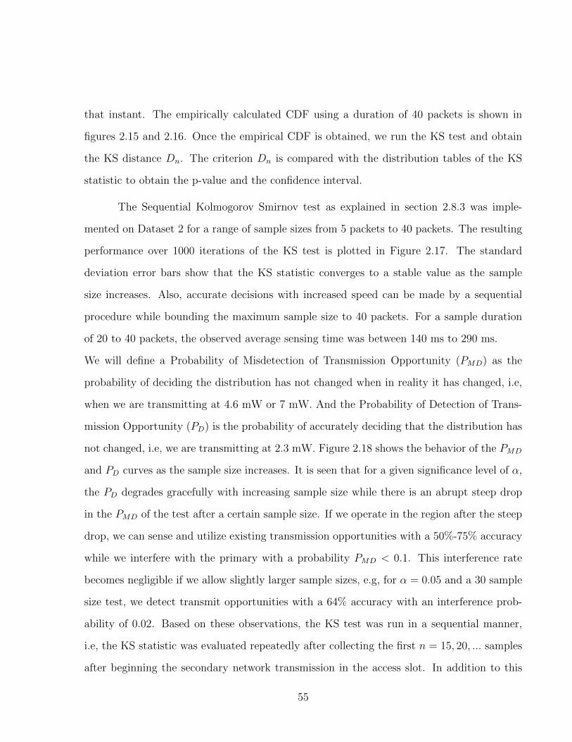
that instant. The empirically calculated CDF using a duration of 40 packets is shown in
figures 2.15 and 2.16. Once the empirical CDF is obtained, we run the KS test and obtain
the KS distance Dn. The criterion Dn is compared with the distribution tables of the KS
statistic to obtain the p-value and the confidence interval.
The Sequential Kolmogorov Smirnov test as explained in section 2.8.3 was imple-
mented on Dataset 2 for a range of sample sizes from 5 packets to 40 packets. The resulting
performance over 1000 iterations of the KS test is plotted in Figure 2.17. The standard
deviation error bars show that the KS statistic converges to a stable value as the sample
size increases. Also, accurate decisions with increased speed can be made by a sequential
procedure while bounding the maximum sample size to 40 packets. For a sample duration
of 20 to 40 packets, the observed average sensing time was between 140 ms to 290 ms.
We will define a Probability of Misdetection of Transmission Opportunity (PMD) as the
probability of deciding the distribution has not changed when in reality it has changed, i.e,
when we are transmitting at 4.6 mW or 7 mW. And the Probability of Detection of Trans-
mission Opportunity (PD) is the probability of accurately deciding that the distribution has
not changed, i.e, we are transmitting at 2.3 mW. Figure 2.18 shows the behavior of the PMD
and PD curves as the sample size increases. It is seen that for a given significance level of α,
the PD degrades gracefully with increasing sample size while there is an abrupt steep drop
in the PMD of the test after a certain sample size. If we operate in the region after the steep
drop, we can sense and utilize existing transmission opportunities with a 50%-75% accuracy
while we interfere with the primary with a probability PMD < 0.1. This interference rate
becomes negligible if we allow slightly larger sample sizes, e.g, for α = 0.05 and a 30 sample
size test, we detect transmit opportunities with a 64% accuracy with an interference prob-
ability of 0.02. Based on these observations, the KS test was run in a sequential manner,
i.e, the KS statistic was evaluated repeatedly after collecting the first n = 15, 20, ... samples
after beginning the secondary network transmission in the access slot. In addition to this
55
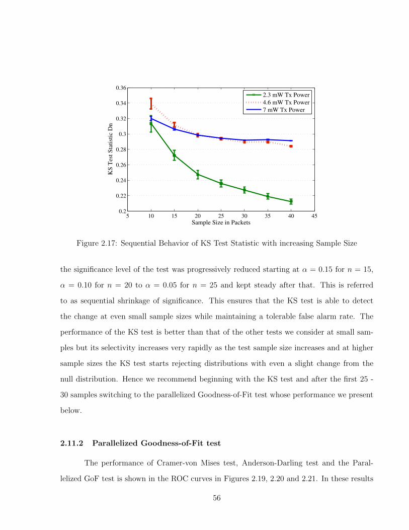
5 10 15 20 25 30 35 40 450.2
0.22
0.24
0.26
0.28
0.3
0.32
0.34
0.36
Sample Size in Packets
KS
Tes
t S
tati
stic
Dn
2.3 mW Tx Power
4.6 mW Tx Power
7 mW Tx Power
Figure 2.17: Sequential Behavior of KS Test Statistic with increasing Sample Size
the significance level of the test was progressively reduced starting at α = 0.15 for n = 15,
α = 0.10 for n = 20 to α = 0.05 for n = 25 and kept steady after that. This is referred
to as sequential shrinkage of significance. This ensures that the KS test is able to detect
the change at even small sample sizes while maintaining a tolerable false alarm rate. The
performance of the KS test is better than that of the other tests we consider at small sam-
ples but its selectivity increases very rapidly as the test sample size increases and at higher
sample sizes the KS test starts rejecting distributions with even a slight change from the
null distribution. Hence we recommend beginning with the KS test and after the first 25 -
30 samples switching to the parallelized Goodness-of-Fit test whose performance we present
below.
2.11.2 Parallelized Goodness-of-Fit test
The performance of Cramer-von Mises test, Anderson-Darling test and the Paral-
lelized GoF test is shown in the ROC curves in Figures 2.19, 2.20 and 2.21. In these results
56

10 15 20 25 30 35 40 45 500
0.1
0.2
0.3
0.4
0.5
0.6
0.7
0.8
0.9
1
Sample Size in Packets
Pro
b. of M
isD
ete
ction/ P
rob. of D
ete
ction
Pd for 2.3mWalpha = 0.15
Pmd for 4.6mWalpha = 0.15
Pmd for 7mWalpha = 0.15
Pd for 2.3mWalpha = 0.10
Pmd for 4.6mWalpha = 0.10
Pmd for 7mWalpha = 0.10
Pd for 2.3mWalpha = 0.05
Pmd for 4.6mWalpha = 0.05
Pmd for 7mWalpha = 0.05
Figure 2.18: ROC Curves for KS Test
Figure 2.19: ROC Curves for AD Test
57

Figure 2.20: ROC Curves for CvM Test
PMD is the probability of misdetection of a transmit opportunity when it exists, that is,
when the CR wrongly decides that it is not safe to transmit. PD is the probability of de-
tection where the CR correctly detects that it transmitting above the transmit margin and
backs off. At very small sample sizes, these tests have a very high probability of classifying
a valid transmit opportunity as not being valid as is seen in the plots. Also as expected,
the Cramer-von Mises test performs better than the Anderson-Darling test when there is a
change in the center region of the packet statistics, which occurs for transmit powers of less
than 80 µW (400 units) while at powers equal to or above this transmit margin, the change
in the density occurs predominantly in the lower tail region and the Anderson-Darling test
shows superior performance. As shown in Figure 2.21 which combines the implementation
of these two tests, the Parallelized Goodness of Fit test performs well for all transmit power
levels. The critical quantity to the primary user is the PD of the test and is bounded to
values above 90 % at all transmit power levels and is often as high as 98-99 % even at small
test duration. On the other hand, the PMD of the test decreases rapidly with the increase in
58
Figure 2.21: ROC Curves for Parallelized Goodness of Fit Test
test duration and saturates at approximately 10% letting us successfully detect and utilize
upto 90% of the available transmit opportunities.
2.11.3 Comparison with the SWIFT approach
In Section 2.2 we discussed the SWIFT approach as presented in [31]. It detects
changes using the Student’s t-test and assumes a Gaussian distribution of the metrics. Figure
2.22 plots the relative performance of the t-test and the Anderson-Darling test which is used
in Protomac. These results are obtained by considering the gaps between successive packet
transmissions as measured by their interarrival times which acts as the network statistic.
It is seen in Figure 2.22a that the Probability of Detection of the Anderson-Darling test is
25 percentage points better than that of the t-test while the AD test Probability of False
Alarm is 10 percentage points better for a test size of 50 samples as in Figure 2.22b. Here
the statistics are assumed to have changed when the KL divergence is at least 0.5. The
underlying non-Gaussianity of the channel interarrival times causes the t-test to show inferior
59
performance to the nonparametric AD test which does not assume any knowledge of the
distribution of the statistics. While the detection performance of Protomac is superior, the
secondary network datarates of SWIFT and Protomac cannot be compared in a fair manner
as SWIFT uses the white space in the unoccupied 5 GHZ ISM bands through a full power
wideband transmission, while Protomac uses the gray space in a single narrowband channel
through a low power transmission. Also, Protomac is designed to prevent the primary users
from switching to another channel due to high secondary interference on current channel,
whereas SWIFT does not check and prevent this behavior, and thus creates artificially vacant
channels by driving away some primary traffic off its channel.
2.12 Experimental Results for Divergence Measure based Tests
2.12.1 Baseline Density Estimates
In Figure 2.12, we have plotted the results of using Deheuvel’s method as explained
in Section 2.9. It shows the kernel density estimates for the different CR transmit powers
in CAP3 dataset. The density estimates are marginally affected by the choice of individual
kernels but show a high sensitivity to the bandwidth chosen. Application of Deheuvel’s
method for CAP3 gave a bandwidths between 62 to 68, while an exhaustive search over the
range 10 to 200 showed optimal performance for bandwidths between 55 to 65. Deheuvel’s
method also performs satisfactorily on CAP1 and CAP2 datasets.
Figure 2.11 plots the accurate densities of the primary packet lengths using the full
duration of the individual captures in the kernel density estimator. The network statistics
do not deviate significantly upto a transmit power level of 600 units. But, there is a sudden
and large shift in the density for transmit power levels of 800 to 1400. Thus, in the case
studied in CAP1 dataset, the Transmit Margin is 600 units. Also, the corresponding metrics
for primary network QOS mirror this threshold. The file transfer rate dropped from 40 kbps
60

(a)
(b)
Figure 2.22: Probability of Detection (a) and Probability of False Alarm (b) for the Student’s
t test and the Anderson-Darling test for increasing test sample size.
61

10 20 30 40 50 60 700
0.1
0.2
0.3
0.4
0.5
Random Sample Window Size
Bha
ttach
aryy
a D
ista
nce
P
Tx = 0
PTx
= 200
PTx
= 400
PTx
= 600
PTx
= 800
PTx
= 1000
PTx
= 1400
(a) Test Performance under i.i.d assumption with random sampling using
Bhattacharyya Distance
10 20 30 40 50 60 700
5
10
15
Random Sample Window Size
KL
Div
erge
nce
PTx
= 0
PTx
= 200
PTx
= 400
PTx
= 600
PTx
= 800
PTx
= 1000
PTx
= 1400
(b) Test Performance under i.i.d assumption with random sampling using
KL Divergence
Figure 2.23: ProTOMAC Results for CAP1 Dataset
62
to 38 kbps at 600 units, 32 kbps at 800 units and 20 kbps at 1000 units. The round trip
delay was unchanged in this case till the transmit power was increased to 1400. Also, the
Transmission Rate remained unchanged at 54 MBps till it dropped to 36 MBps at a power
level of 1000. A similar clear threshold was found for the other datasets. Thus, the Transmit
Margin as predicted by ProTOMAC is slightly conservative.
2.12.2 Tests using Randomized Sampling
Now, we will examine the performance of ProTOMAC under various formulations of
the group sequential type tests as explained in Section 2.6. If we neglect the underlying non-
stationarity and model the data as being drawn from an independent identically distributed
(i.i.d)process, then the best bound for the test performance is obtained as shown in Figure
2.23b for the Bhattacharyya Distance and in Figure 2.23a for the KL Divergence measure. It
demonstrates the behavior of the divergence between the approximate estimated density of
a small size sample and the accurate prechange density as the size of the sample is increased
from 10 to 70 packets. These packets are selected via random uniform sampling without
replacement from the full capture duration. This sampling model is impractical for actual
implementation as we have to wait for the whole duration of the capture before sampling it,
which will introduce a large delay. But the performance under the random sampling model is
a good comparison benchmark. We note from figure 2.23b that the maximum discrimination
between the two densities is possible for the low sample size range, i.e, 20-30 packets, which
is a remarkably fast sensing time.
2.12.3 Group Sequential Test
A highly efficient and fast practical modification of the above random sampling scheme
is to randomly select without replacement a subset of length M out of the N samples captured
till the current instant. This introduces an element of randomization that improves system
63

performance. Figure 2.26 shows the Bhattacharyya distance for CAP1 dataset with fixed
representative random sample lengths of 20, 40 and 100, as plotted in Figures 2.26a, 2.26b and
2.26c respectively, for increasing total capture duration. Also, the corresponding performance
of the KL Divergence measures is plotted in Figures 2.26d, 2.26e and 2.26f. Thus, it is a
group sequential test implementation with a rough density estimate calculated using 20
samples and progressively refined with the addition of consecutive groups of 10 samples
each. During analysis, an empirical threshold of 0.3 for the KL divergence and 3.5 for the
Bhattacharyya distance was used. ProTOMAC shows reliable convergence with time as the
capture duration increases. It was observed that Bhattacharyya Distance based test had an
asymptotic gain of 1.5 while the KL divergence based test had an asymptotic gain of 4. Also,
the test statistic is highly conservative at smaller sample sizes. For example, a threshold of a
Bhattacharyya Distance 0.3 classifies some safe Transmit Opportunities as unsafe for small
capture duration. This classification error reduces rapidly at longer capture duration. Also,
there is faster convergence and a reduction in the degree of risk with increasing random
sample length. Similar results are obtained if we use the KL divergence as a statistic as
shown in Figures 2.26d, 2.26e and 2.26f.
2.12.4 Secondary Link Power Budget
ProTOMAC implements an end-to-end secondary link. A stream of packets is trans-
mitted from SDR 1 to SDR 2 over the secondary channel which has been carved out at
the given Transmit Margin. We will now characterize the secondary link behavior and in-
vestigate the performance and reliability of the secondary network. In each instance a 1
MB file was transmitted as packets of a fixed size over the link. Binary Phase Shift Keying
(BPSK) modulation was implemented with 1 bit per symbol to work at a 500 kbps bitrate.
The carrier frequency for the BPSK was set to 2.412 GHz. Figure 2.25a plots the effect of
increasing the transmit power on the PER, for different fixed packet sizes. Higher packet
64
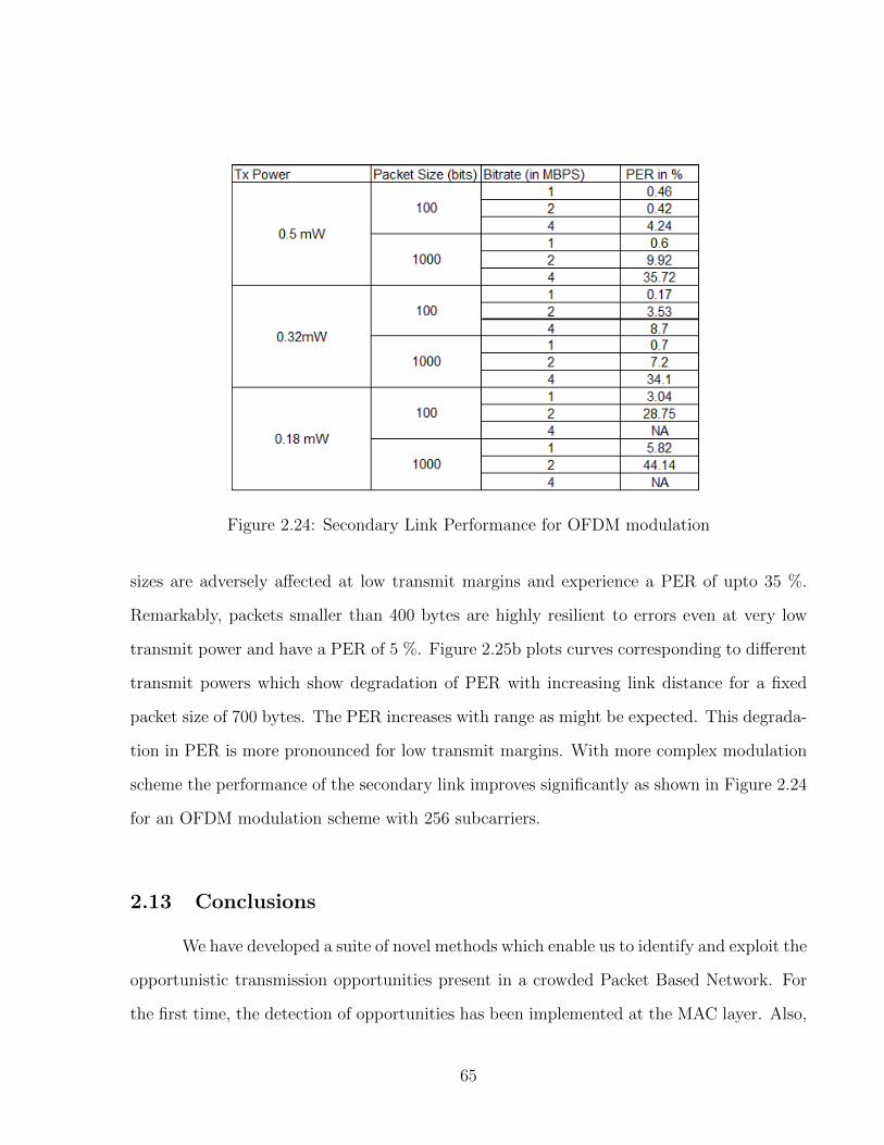
Figure 2.24: Secondary Link Performance for OFDM modulation
sizes are adversely affected at low transmit margins and experience a PER of upto 35 %.
Remarkably, packets smaller than 400 bytes are highly resilient to errors even at very low
transmit power and have a PER of 5 %. Figure 2.25b plots curves corresponding to different
transmit powers which show degradation of PER with increasing link distance for a fixed
packet size of 700 bytes. The PER increases with range as might be expected. This degrada-
tion in PER is more pronounced for low transmit margins. With more complex modulation
scheme the performance of the secondary link improves significantly as shown in Figure 2.24
for an OFDM modulation scheme with 256 subcarriers.
2.13 Conclusions
We have developed a suite of novel methods which enable us to identify and exploit the
opportunistic transmission opportunities present in a crowded Packet Based Network. For
the first time, the detection of opportunities has been implemented at the MAC layer. Also,
65

200 400 600 800 1000 1200 14000
0.05
0.1
0.15
0.2
0.25
0.3
0.35
0.4Packet Size
Transmit Power
Pac
ket E
rror
Rat
e
1500 Bytes1100 Bytes700 Bytes400 Bytes100 Bytes
(a) Effect of Packet Size on Secondary Link Performance for BPSK
modulation: PER vs Tx Power
200 400 600 800 1000 1200 14000.05
0.1
0.15
0.2
0.25
0.3
0.35
0.4
0.45
0.5
Transmit Power
Pac
ket E
rror
Rat
e
Link Range
1 Meter2 Meters3 Meters
(b) Effect of Link Distance on Secondary Link Performance for BPSK
modulation: PER vs Tx Power
Figure 2.25: ProTOMAC Results for CAP1 Dataset
66

50 100 150 200 250 3000
0.1
0.2
0.3
0.4
0.5
0.6
0.7
Sample Length
Bha
ttach
aryy
a D
ista
nce
len = 20
PTx
= 0
PTx
= 200
PTx
= 400
PTx
= 600
PTx
= 800
PTx
= 1000
PTx
= 1400
(a) N=20
50 100 150 200 250 3000
0.1
0.2
0.3
0.4
0.5
0.6
0.7
Sample Length
Bha
ttach
aryy
a D
ista
nce
len = 40
P
Tx = 0
PTx
= 200
PTx
= 400
PTx
= 600
PTx
= 800
PTx
= 1000
PTx
= 1400
(b) N=40
50 100 150 200 250 3000
0.1
0.2
0.3
0.4
0.5
0.6
0.7
Sample Length
Bha
ttach
aryy
a D
ista
nce
100
P
Tx = 0
PTx
= 200
PTx
= 400
PTx
= 600
PTx
= 800
PTx
= 1000
PTx
= 1400
(c) N=100
50 100 150 200 250 3000
2
4
6
8
10
12
14
16
Sample Length
KL
Div
erge
nce
P
Tx = 0
PTx
= 200
PTx
= 400
PTx
= 600
PTx
= 800
PTx
= 1000
PTx
= 1400
(d) N=20
50 100 150 200 250 3000
2
4
6
8
10
12
14
16
Sample Length
KL
Div
erge
nce
80
P
Tx = 0
PTx
= 200
PTx
= 400
PTx
= 600
PTx
= 800
PTx
= 1000
PTx
= 1400
(e) N=40
50 100 150 200 250 3000
2
4
6
8
10
12
14
16
Sample Length
KL
Div
erge
nce
P
Tx = 0
PTx
= 200
PTx
= 400
PTx
= 600
PTx
= 800
PTx
= 1000
PTx
= 1400
(f) N=100
Figure 2.26: Group Sequential Test Performance for CAP1 Dataset using Bhattacharyya
Distance as Metric67
the primary network QoS is safeguarded and the interference constraints are obeyed using the
Transmit Margin that we have introduced. We have implemented our method in a real world
large scale IEEE 802.11 WLAN and successfully established a reliable Secondary link between
two nodes. Although we have made a number of assumptions like a quasi-stationarity of the
packet statistics on a medium time scale, we have practically demonstrated the soundness
and viability of the metrics used. Thus, we have achieved significant utilization of hitherto
unused transmit opportunities. We hope to have introduced a new domain of cognition for
CRNs which shows exciting potential for novel applications.
68

Chapter 3
Phi-divergence based Ensemble Goodness of Fit tests
3.1 Introduction
The problem of inference based decision making is conventionally treated as that of
hypothesis testing for parametric models where the distributions are modeled using known
and parametric probability functions which usually belong to the exponential family of dis-
tributions. Such a framework has worked remarkably well in the past including in a series
of recent applications where the hypotheses to be tested are not well defined. Also, the
robustness of parametric tests is often inferior to that of equivalent non parametric tests
when there is uncertainty in the knowledge of the noise statistics or when the noise statis-
tics are non-parametric. The penalty usually incurred for this increase in robustness is a
decrease in the power of the test. Goodness of Fit tests are a particularly popular and ro-
bust class of inferential tests that have been applied for almost a century in the statistical
community [41, 64]. But, the use of these tests in digital communications applications has
historically been restricted to testing the fit of empirical models to data, i.e, model fitting.
Recently, there has been an effort to study the performance of these tests for hypothesis
testing applications, and highly encouraging results have been obtained [65–67].
3.1.1 Our Contributions
This work makes four major contributions towards developing ensemble phi-divergence
based tests for spectrum sensing.
69

1. First, a generalized framework for inferential decision making based on phi-divergences
is presented. It is shown how many other conventional goodness of fit measures are
special cases of these statistics and the tailored design of new tests having desirable
properties is introduced.
2. Second, extensive simulation results of the performance of this family of tests under
Gaussian as well as non-Gaussian (impulsive) noise environments are presented.
3. Third, we develop a novel decision fusion method based on the statistical nature of
the p-value metric that shows robust and predictable performance under variability in
noise distributions.
4. Fourth, the combination of spatially separated tests under the assumption of inde-
pendent but not necessarily identically distributed underlying distributions is studied,
using a new summary test statistic.
There are two primary reasons for adopting a non-parametric goodness-of-fit test.
First, it has a significantly reduced computational load as compared to complex parametric
tests such as cyclostationarity detection [68], Maximum Likelihood detection, eigenvalue
based detection [69] etc. No matrix inversions or Fourier transforms are needed. Instead,
a simple distribution calculation followed by the use of a lookup table suffices. Second,
such tests are inherently highly robust in the presence of unreliable information on the
distributions under the hypothesis. Moreover, they work as well in the presence of completely
arbitrary distributions. Third, the tests deliver satisfactory small sample performance, which
allows the designer to effectively trade off performance versus sensing duration if desired.
These tests have a number of other desirable properties that will be apparent in later sections.
70

3.1.2 Related Work
3.1.2.1 Non Parametric Statistics in Communications
Although parametric estimation and detection methods comprise the majority of pro-
posed methods in digital communications, a significant variety of non-parametric statistical
approaches coexist with them. There is a rich history of work, starting with the classical
bibliography in [70] to recent works [68, 71, 72], but unlike the proposed work these cannot
be applied to the use of goodness-of-fit tests nor to their distributed versions.
3.1.2.2 Goodness of Fit tests in Cognitive Radio literature
In this section we will review the use of Goodness-of-Fit tests in the literature. We
will focus on aspects of hypothesis testing where the application domain is the problem of
sensing white spaces in dynamic spectrum access systems [13, 73]. In [33, 65], a fast and
robust spectrum sensing scheme is proposed using the Kolmogorov-Smirnov goodness of fit
test. It is demonstrated through simulations that the KS test offers superior performance
in and faster signal detection times as compared to traditional methods such as energy
detection, eigenvalue-based detection and cyclostationarity detection. In the presence of a
Gaussian noise, the KS test has been shown to be highly robust to uncertainty in background
noise estimation as compared to the energy detection. Moreover, its performance is superb
in the presence of non-Gaussian noise also, where other spectrum sensing methods often
fail. The main drawback in their approach is that their interpretation of a goodness of
fit test as a binary hypothesis test has been questioned in the statistical literature [74, 75].
Goodness-of-Fit tests are not meant to accept the null hypothesis H0, but only reject it at a
certain significance level. In other words, all the Kolmogorov-Smirnov test states is that the
hypothesis that the noise is modeled by the estimated noise density can be rejected with a
confidence level of α (usually 99.5 % etc ). In contrast to the above mentioned approaches, our
71

proposed use of testing the uniformity of p-values for phi-divergence test does not encounter
these conceptual difficulties. The test statistic can also exceed the threshold when either a)
the assumed noise model is wrong as often happens in presence of impulsive non-Gaussian
noise or b) there is another very weak non primary interferer that is subtly changing the
noise distribution from the theoretical one. The latter situation can be treated using an
approach similar to the techniques to detect sparse heterogeneity in mixtures and we will
not consider that here [76] We will focus only on the first case in the rest of this chapter
since in spectrum sensing applications the mischaracterization of noise statistics is the main
problem.
Also, [66] recently proposed a Anderson Darling version of goodness of fit test for
spectrum sensing but do not apply it to non-Gaussian noise models. The problem of reliable
detection of gray space transmit opportunities using goodness-of-fit and other non-parametric
techniques has been previously studied by the authors of this work [32–34] and by others [31]
in the context of the Medium Access layer packet statistics.These works use only a single
fixed Goodness-of-Fit test. Our proposed approach is significantly different in two ways, it
uses an ensemble of tunable Goodness-of-Fit tests, and it reformulates the problem into a
test for uniformity of p-values.
3.2 Inference Problem Formulation
We apply the proposed methods to the following inference problem. Consider the
scenario where an unlicensed cognitive radio is trying to detect the presence of a licensed
primary user via spectrum sensing. We model the general case where both the primary and
secondary users have multiple antennas. Specifically, the MIMO channel is created by MT
transmit antennas and MR receive antennas. We can express the generalized discrete-time
72
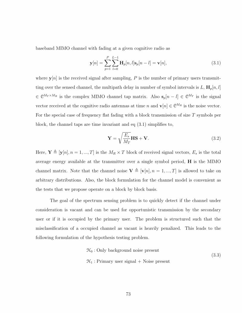
baseband MIMO channel with fading at a given cognitive radio as
y[n] =P∑p=1
L−1∑l=0
Hp[n, l]sp[n− l] = v[n], (3.1)
where y[n] is the received signal after sampling, P is the number of primary users transmit-
ting over the sensed channel, the multipath delay in number of symbol intervals is L, Hp[n, l]
∈ CMT×MR is the complex MIMO channel tap matrix. Also sp[n − l] ∈ CMT is the signal
vector received at the cognitive radio antennas at time n and v[n] ∈ CMR is the noise vector.
For the special case of frequency flat fading with a block transmission of size T symbols per
block, the channel taps are time invariant and eq (3.1) simplifies to,
Y =
√EsMT
HS + V. (3.2)
Here, Y , [y[n], n = 1, ..., T ] is the MR × T block of received signal vectors, Es is the total
average energy available at the transmitter over a single symbol period, H is the MIMO
channel matrix. Note that the channel noise V , [v[n], n = 1, ..., T ] is allowed to take on
arbitrary distributions. Also, the block formulation for the channel model is convenient as
the tests that we propose operate on a block by block basis.
The goal of the spectrum sensing problem is to quickly detect if the channel under
consideration is vacant and can be used for opportunistic transmission by the secondary
user or if it is occupied by the primary user. The problem is structured such that the
misclassification of a occupied channel as vacant is heavily penalized. This leads to the
following formulation of the hypothesis testing problem.
H0 : Only background noise present
H1 : Primary user signal + Noise present
(3.3)
73
3.3 Phi-Divergence based Goodness-of-Fit Tests
3.3.1 Goodness-of-Fit Procedures
A goodness-of-fit test is a procedure for testing how well a certain distribution fits a
given observation [41, 64]. To be more specific, consider a continuous random variable X with
distribution F(x) and let X1, X2, ..., Xn be a random sample of independent and identically
distributed random variables each following distribution F(x), with order statistics X(1) ≤
X(2) ≤ ... ≤ X(n). To implement a goodness-of-fit test, we modify eq (3.3) to
H0 : F(x) = F0(x) (Null hypothesis),
H1 : F(x) 6= F0(x) (Alternative hypothesis).
(3.4)
Here F0(x) is the hypothesized null distribution function to be tested. The alternative
hypothesis is transformed into a composite hypothesis that is defined as the complement of
the null hypothesis. Although we consider the simple null hypothesis for the most parts, it is
straightforward to extend the methods to the case of a composite null hypothesis where F0(x)
has parameters θ0 ∈ Ω0 We note here that the goodness-of-fit testing procedure is closely
related to the tests for such universal hypotheses in information theory. The Empirical
Distribution Function (edf) of X is defined as
Fn(x) =1
n
n∑i=1
1I(Xi < x), −∞ < x <∞ (3.5)
where 1I(.) is the indicator function that evaluates to 1 if the condition in the braces
is true, and is 0 otherwise. Also, the probability integral transformation theorem is stated
below. The edf as defined in eq (3.5) combined with the probability integral transformation
theorem leads directly to a number of powerful goodness-of-fit tests. See [77] for a generalized
proof of the theorem.
Theorem 1. Probability Integral Transformation
Let a random variable X have a distribution F(x). If F is continuous, the random variable
74

Z produced by a transformation Z = F(X) has a uniform probability distribution over the
interval 0 ≤ z ≤ 1.
3.3.2 Phi-Divergences
In the rest of this chapter we propose a novel use of Phi-Divergences for the purpose of
inference between two hypotheses. It has recently been shown that Phi Divergences are the
optimal formulations for goodness-of-fit testing [78–81]. Many previous goodness-of-fit tests
that have been proposed can be reduced to specialized cases of the phi-divergence statistic.
Also, the Phi-Divergences can also be modified to include the standard distributional diver-
gence measures like Kullback-Leibler divergence, Jensen divergence etc. Thus they provide
a link between the metrics used for inference in statistical information theory and the non
parametric inferential techniques used in goodness of fit based approaches. We will capitalize
on these generalizations to allow us to come up with a wide and powerful family of goodness
of fit statistics, out of which the best suited test can be chosen, using guidelines that we
subsequently provide.
Let φ(x) be a convex function with domain x ∈ [0,∞) and range < ∪ ∞. Then
the supremum and integral versions of the Jager-Wellner Generalized Phi Divergences will
be defined as
Sn(φ) = supxKφ
(Fn(x), x
), (3.6)
Tn(φ) =
∫ 1
0
Kφ
(Fn(x), x
)dx. (3.7)
To allow us to draw parallels to various information theoretic divergence measures
and statistical goodness-of-fit tests, we will restrict ourselves to the following special class of
φ-functions using the parameter s ∈ <
75

φs(x) =
[1− x− sx− xs]/[s(1− s)] s 6= 0, 1
x(log x− 1) + 1 s = 1,
log(1/x) + x− 1 s = 0.
(3.8)
Also, with the kernel function used in eq (3.6) defined as in eq (3.9), we get the family
of φs-divergences.
Ks(u, v) = vφs(u/v) + (1− v)φs([1− u]/[1− v]) (3.9)
After substituting φs(x) as defined in eq (3.8) into eq (3.9) above, we get,
Ks(u, v) =1
s(1− s)
(1− usv1−s − (1− u)s(1− v)1−s
). (3.10)
Here, φs is continuous in s∀x ∈ (0, 1) and Ks is continuous in s ∀ (u, v) ∈ (0, 1)2. For each
s, we obtain a unique goodness-of-fit test. It can be shown that a variety of previously
proposed powerful goodness-of-fit tests can be obtained as described next.
3.3.3 Relation of Φ-Divergence Statistics to other Goodness-of-Fit Statistics
Φ-Divergence Statistics can be shown to include many other commonly used statistical
tests as special cases. We will state a few special cases along with references for a more
detailed treatment.
For s = 2, the Φ-divergence statistic Sn(2) is proportional to the supremum form of the
Anderson-Darling statistic [76].
For s = 1, the Φ-divergence statistic Sn(1) reduces to the Berk-Jones statistic and for s = 0,
it reduces to the reversed Berk-Jones statistic [82–84].
For s = 1, the Φ-divergence statistic Tn(1) is the intergral version of the Berk-Jones statistic
[85].
76

0 0.1 0.2 0.3 0.4 0.5 0.6 0.7 0.8 0.9 10
0.5
1
1.5
2
2.5
3
3.5
4
4.5
5
Φs (x) functions for s = −1 to 2
s = −1
s = −0.5
s = 0
s = 0.5
s = 1
s = 1.5
s = 2
Figure 3.1: Φ function plots
For s = 2, the Φ-divergence statistic Sn(1) reduces to the classical Anderson-Darling statistic.
The corresponding Φ-divergence kernels are,
K0(u, v) = v logu
v+ (1− v) log
1− u1− v
. (3.11)
K1(u, v) = u logu
v+ (1− u) log
1− u1− v
. (3.12)
K2(u, v) =1
2
(u− v)2
v (1− v). (3.13)
77
3.4 Phi-Divergence Tests for Spectrum Sensing
3.4.1 Handling Non-Gaussian Noise
Radio Frequency Interference (RFI) is a severe issue in modern spectrum sensing
applications. The primary sources of RFI are non-communication sources of radiation such as
microwave ovens, other wireless systems which are in close proximity, and the computational
platform sources such as clock circuitry, co-located transceivers and power amplifiers which
produce phase noise, clock offset noise etc. Ignoring RFI can lead to spurious decisions in
favor of the signal being present, due to the impulsive noise. The non-parametric nature
of the goodness-of-fit test becomes advantageous when there is such type of added RFI
front end noise that is non-Gaussian in nature. The performance of conventional detection
techniques degrades severely under such conditions, whereas as we show, the GoF tests are
robustly able to handle such noise with minimum effect on performance.
Middleton Class A,B and C noise models are the most widely adopted non-Gaussian
noise model and have been proven to model the non-Gaussianity accurately. We follow the
bivariate Middleton Class A noise model as proposed in [86–88], which also explicitly ac-
counts for the standard thermal noise through an additive Gaussian component. Narrowband
impulsive noise is modeled as a series of independent events that are identically distributed.
Also, the in-phase and quadrature components are usually modeled as i.i.d. The cases we
will study here are
1. Magnitude based 1-D KS test with Gaussian noise
2. Magnitude based 1-D KS test with Middleton Class-A noise
3. Φ-Divergence based test with Gaussian noise for s ∈ [−1, 2].
4. Φ-Divergence based test with Middleton Class-A noise for s ∈ (−1, 2).
78
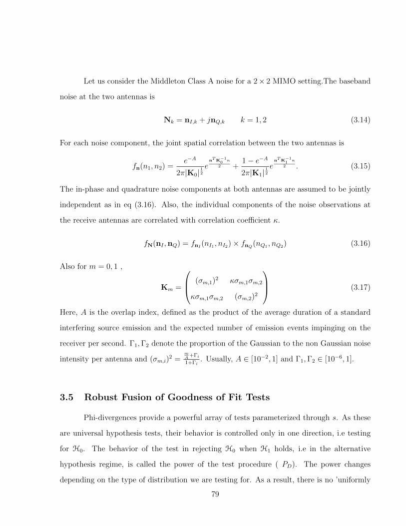
Let us consider the Middleton Class A noise for a 2× 2 MIMO setting.The baseband
noise at the two antennas is
Nk = nI,k + jnQ,k k = 1, 2 (3.14)
For each noise component, the joint spatial correlation between the two antennas is
fn(n1, n2) =e−A
2π|K0|12
enTK−1
0 n
2 +1− e−A
2π|K1|12
enTK−1
1 n
2 . (3.15)
The in-phase and quadrature noise components at both antennas are assumed to be jointly
independent as in eq (3.16). Also, the individual components of the noise observations at
the receive antennas are correlated with correlation coefficient κ.
fN(nI ,nQ) = fnI(nI1 , nI2)× fnQ
(nQ1 , nQ2) (3.16)
Also for m = 0, 1 ,
Km =
(σm,1)2 κσm,1σm,2
κσm,1σm,2 (σm,2)2
(3.17)
Here, A is the overlap index, defined as the product of the average duration of a standard
interfering source emission and the expected number of emission events impinging on the
receiver per second. Γ1,Γ2 denote the proportion of the Gaussian to the non Gaussian noise
intensity per antenna and (σm,i)2 =
mA
+Γi
1+Γi. Usually, A ∈ [10−2, 1] and Γ1,Γ2 ∈ [10−6, 1].
3.5 Robust Fusion of Goodness of Fit Tests
Phi-divergences provide a powerful array of tests parameterized through s. As these
are universal hypothesis tests, their behavior is controlled only in one direction, i.e testing
for H0. The behavior of the test in rejecting H0 when H1 holds, i.e in the alternative
hypothesis regime, is called the power of the test procedure ( PD). The power changes
depending on the type of distribution we are testing for. As a result, there is no ’uniformly
79

00.2
0.40.6
0.81
0
0.5
1
0
1
2
3
4
uv
K (
u,v
)
Figure 3.2: K(u,v) with s= 1/2
00.2
0.40.6
0.810
0.5
10
1
2
3
4
5
uv
K (
u,v
)
Figure 3.3: K(u,v) with s=1
most powerful’ test from such a non-parametric setting, and different tests will be locally
the most powerful, for a given set of alternate distributions. Depending on the structure
of the distribution under the alternate hypothesis, the different goodness-of-fit tests vary
80

00.2
0.40.6
0.810
0.5
10
10
20
30
40
50
uv
K(u
,v)
Figure 3.4: K(u,v) with s=2
greatly in power. Thus it is not possible to recommend a single test as an omnibus test
over a range of SNRs as its performance may be surpassed by another test under different
operating conditions.In cognizance of this fact, we propose to apply a battery of tests with
uniformly spaced s using a novel Thresholded Extreme Value test. In this section, we will
develop methodologies for the proper combination of such tests. Our results show that the
combined test consistently outperforms individual tests, including the Kolmogorov Smirnov
test. Our proposed Thresholded Extreme Value test is based on the following properties of
the p-value.
3.5.1 p-value
In statistics, the p-value of a test is defined as the tail integral of the density of the
test statistic. Consider a goodness-of-fit test with a test statistic T (X). Let ZT (t) and
WT (t) be the cumulative distributions of T under the null hypothesis (H0) and alternative
hypothesis (H1) respectively. Then for a given observed test statistic T (X) = τ , the p-value
81

0 0.05 0.1 0.15 0.2 0.25 0.3 0.35 0.4 0.45 0.50
2
4
6
8
10
12
14
Test Statistic
p.d
.f
H0
H1
(a)
0 0.1 0.2 0.3 0.4 0.5 0.60
2
4
6
8
10
12
14
H0
H1
(b)
−0.5 0 0.5 1 1.5 2 2.5 30
2
4
6
8
10
12
14
16
18
Test Statistic
p.d
.f
H0
H1
(c)
0.05 0.1 0.15 0.2 0.25 0.30
2
4
6
8
10
12
14
Test Statistic
p.d
.f
H0
H1
(d)
0 0.05 0.1 0.15 0.2 0.25 0.3 0.350
2
4
6
8
10
12
14
Test Statistic
p.d
.f
H0
H1
(e)
0 0.2 0.4 0.6 0.8 1 1.20
2
4
6
8
10
12
14
16
Test Statistic
p.d
.f
H0
H1
(f)
Figure 3.5: Distributions of the test statistics for the KL test and Phi-Divergence test
of the test is given as,
ρ(τ) = supθ∈Ω0
P(T (X) ≥ τ) (3.18)
For the special case of a simple null hypothesis,
ρ(τ) = P(T > τ |H0) = 1− ZT (τ) =
∫ +∞
τ
zT (t) dt. (3.19)
The p-value acts as an indicator of the confidence of the decision reached by the
goodness-of-fit test. A low p-value indicates that we are highly unsure about rejecting the
null hypothesis while a high p-value indicates that we are highly confident in rejecting the
null hypothesis. For our purposes, the principle utility is that the p-value is obtained via
an implicit probability integral transformation as we show in the Theorem below. As the
p-values are distributed uniformly over [0, 1] under the null hypothesis, we will compare the
outputs of different types of goodness-of-fit tests that have mismatched ranges of their test
statistics on a standardized [0, 1] interval.
82

Theorem 2. p-value distribution property
The distribution of p-values for the null hypothesis is uniform over [0,1] for
any test sample size.
Proof. Using the definition of p-value as in equation (3.19),
F%(ρ|H0) = P(% ≤ ρ) (3.20)
= P
(1− ZT (τ)
)≤ ρ
(3.21)
= 1− ZTZ−1T (1− ρ)
(3.22)
= ρ. (3.23)
∴ F%(ρ|H0) ∼ U[0, 1] (3.24)
3.5.2 Ensemble of Φ-Divergence Test test
The Kolmogorov Smirnov test, Anderson-Darling test and other standard goodness-
of-fit tests are individually sensitive to changes only in certain regions of the distribution
and sacrifice high local power in order to attain medium power over the complete support of
the cumulative distribution function (c.d.f). In contrast, the Φ-Divergence tests have been
designed to be selective to changes in different regions of the c.d.f, and this selectivity is
controlled via the tuning parameter s. Hence, the ensemble demonstrates a rake like property
by being highly sensitive to changes over the complete support of the c.d.f. We have seen
that the p-value measures the confidence of a given test under a set of specific operating
conditions. Our approach is based on the observation in [89] that the distribution of the p-
value under both hypothesis is essential to formulate a threshold. Out of the ensemble of the
goodness-of-fit tests,we accept the decision of the test that has the most extreme p-value, i.e
83

0 0.1 0.2 0.3 0.4 0.5 0.6 0.7 0.8 0.9 10
1
2
3
4
5
6
7
8
p−value
p.d
.f
H0
H1
Figure 3.6: Distribution of p-values under H1 and H0 for SNR = -2 dB, test size = 50
, it has the highest confidence metric to support the decision. We will illustrate the process
using the distribution of the p-values for SNR = 0 case, for the setup described in Results
section. The distribution of p-values for the ensemble of tests is plotted in figure 3.6. The
uniformity of the p-values under the null hypothesis is clearly seen, also the distribution
under the alternative is highly skewed towards 0. The level of significance α to reject the
null hypothesis is easily noted to be p-value = α. We will calculate a second order P-value
defined as the upper tail integral of the alternate p-value distribution and threshold it a
level β. Note that this differs from conventional p-value use in that the threshold depends
via β on the distribution under the alternate hypothesis. After these rejection regions have
been defined, the remaining area is subject to a randomized test (see Chp.3 , Lehmann [90]
for a review of the randomized test concept). The randomized test randomly decides the
outcome after normalizing with a predetermined prior distribution of the two hypothesis
in the randomization region. Thus, the Ensemble Goodness-of Fit (EG) test based on Φ-
Divergences is implemented as follows
84

Figure 3.7: Block Diagram of Ensemble Goodness-of-Fit tests using tunable Phi-divergence
statistics
1. Training phase: Calculate the distribution of p-values of all the test statistics under
Null and Alternate hypotheses. Calculate the rejection region and the randomization
region.
2. Test Phase: For the test sample, obtain test statistics for each test in the ensemble,
and the corresponding p-values.
3. If the test p-value falls within a rejection region, pick the corresponding hypothesis.
4. Otherwise, randomly pick the hypothesis using the prior distribution and the magni-
tude of p-value.
5. If any test rejects the null hypothesis, then the EG test decides in favor of H1.
The consistently superior performance of this test is shown via experimental simula-
tions in section 3.7. Here, we describe the rationale behind this particular approach.
85

−12 −10 −8 −6 −4 −2 00
0.1
0.2
0.3
0.4
0.5
0.6
0.7
0.8
0.9
1
SNR
Pro
ba
bility o
f D
ete
ctio
n
TEV Test
KS Test
ED Test
(a)
−12 −10 −8 −6 −4 −2 00
0.1
0.2
0.3
0.4
0.5
0.6
0.7
0.8
0.9
1
SNR
Pro
bability o
f D
ete
ction
TEV Test
KS Test
ED Test
(b)
−12 −10 −8 −6 −4 −2 00.2
0.3
0.4
0.5
0.6
0.7
0.8
0.9
1
SNR
Pro
bability o
f F
als
e A
larm
EG Test
KS Test
ED Test
(c)
−12 −10 −8 −6 −4 −2 0
0.05
0.1
0.15
0.2
0.25
0.3
SNR
Pro
bability o
f F
als
e A
larm
TEV Test
KS Test
ED Test
(d)
−12 −10 −8 −6 −4 −2 00
0.05
0.1
0.15
0.2
0.25
0.3
0.35
Pro
bability o
f F
als
e A
larm
SNR
TEV Test
KS Test
ED Test
(e)
−12 −10 −8 −6 −4 −2 00
0.05
0.1
0.15
0.2
0.25
0.3
0.35
SNR
Pro
bability o
f F
als
e A
larm
EG Test
KS Test
ED Test
(f)
Figure 3.8: Performance of the various tests for test size = 50. Fig 3.8a : PD for Gaussian
noise, Fig 3.8b : PD for Non-Gaussian noise with Γ = 0.5 , Fig 3.8d : PFA for Gaussian
noise, Fig 3.8e : PFA for non-Gaussian noise, Fig 3.8f : PFA for Non-Gaussian noise with
Γ = 0.1
86

Definition 1. Consider random variables X and Y with cumulative distribution functions
FX and FY . Then, FX will be said to stochastically dominate FY at the first order (FY (y) 1
FX(y)) if and only if FY (y) ≥ FX(y) ∀y. FX strictly dominates FY with the first order if
and only if FY (y) ≥ FX(y) ∀ y and ∃y s.t FY (y) > FX(y)
Similarly, higher orders of stochastic dominance are defined on repeated integrals of
the cumulative distribution as shown below. Using the definition of stochastic dominance
and of rejection region, we can prove the following theorem.
Definition 2. FX will be said to stochastically dominate FY at the second order (FY (y) 2
FX(y)) if and only if ∫ t
0
FY (x) dx ≥∫ t
0
FX(x) dx ∀t (3.25)
Lemma 1. First order stochastic dominance implies second order stochastic dominance.
Proof. Rearrange equation(3.25) as∫ t
−∞(FY (x)− FX(x)) dx ≥ 0 ∀t. (3.26)
. This is obviously true as first order dominance implies
FY (x) ≥ FX(x) ∀x (3.27)
Now consider the ensemble goodness-of-fit test of size G, where the class of alternate
hypothesis is right-tailed such that the expectation of the test statistic is larger under the
alternate hypothesis than under the null hypothesis. Thus,
F1,i 1 F0,i i = 1, ..., G. (3.28)
87
By Lemma 1 F0 also dominates F1 at the second order, i.e, F1 2 F0. Also, by
Theorem 2, F0,i ∼ U(0, 1)∀i ∈ 1, ..., G. Thus,
F1,i 1 U i = 1, ..., G. (3.29)
where, U ∼ U(0, 1).
Thus for an ensemble of tests, we will define a piecewise alternate distribution using
the method as shown below.
F1,alt(y) = maxi=1,..,G
F1,i(y)∀y ∈ [0, 1]. (3.30)
This can be seen to be the convex hull of the individual p-value distributions under the alter-
nate hypothesis. Doing so does not affect the behavior of the test under the null hypothesis,
as the c.d.f is a uniform distribution as per Theorem above. Thus, by construction, this ef-
fective alternate distribution is stochastically dominant over all individual alternate distribu-
tions of the p-values in the ensemble. Hence, the performance of the ensemble goodness-of-fit
test is superior to all its constituent tests.
Lemma 2. The expectation of the p-value of the test under the alternative hypothesis is
smaller than the expectation of the p-value of the test under the null hypothesis.
Theorem 3. If the test is unbiased, the c.d.f of the test statistic under the null hypothe-
sis is always stochastically dominant over the c.d.f of the test statistic under the alternate
hypothesis.
3.5.3 Choice of Ensemble GoF test parameters
We will now give guidelines to design the ensemble Goodness-of-Fit test for a specific
situation. The baseline test is the Kolmogorov-Smirnov test which is moderately sensitive
to changes over the complete support for the density functions. If we known the exact
88

parametric form of the densities under the null and alternate hypotheses, then we can design
a test that is tuned to the region of maximum change. In the absence of this knowledge,
which is the situation studied here, the following guidelines allow us to design an ensemble
Goodness-of-Fit test that delivers a good performance. The aim is to have the minimum
number of tests in the ensemble to manage the implementation complexity.
1. Start with 3 tests for s = −1, 0, 1 that are sensitive to a change in left and right tails
as well as the median of the density. This simple ensemble is sufficient for symmetric
and relatively smooth densities.
2. Check if the performance of the ensemble is consistently improved over that of the
baseline Kolmogorov-Smirnov test alone.
3. Gradually keep adding more tests to the ensemble to cover more and more regions of the
densities till required performance is achieved. Note that we restrict the searchspace to
values of s = 0.5n where n = −2...4 which have been implemented in the R statistical
software.
Summarizing the properties of the Ensemble Goodness-of-Fit test, we note that it
first implements a parallelized ensemble of basic goodness-of-fit test, and then it reformulates
this ensemble into a collection of p-values of the constituent tests. This reformulation allows
us to test the goodness-of-fit for the uniformity of p-values. Thus we have decoupled the
proposed ensemble test design and the design of the constituent goodness-of-fit test. Also,
the theorem above shows the divergent behavior of the p-value distribution under the null
and alternate hypotheses and this implies that the test will always function correctly. The
exact performance gains delivered by the proposed test is shown in the Results section
89

−12 −10 −8 −6 −4 −2 00
0.1
0.2
0.3
0.4
0.5
0.6
0.7
0.8
0.9
1
SNR
Pro
ba
bili
ty o
f D
ete
ctio
n
CSS EG Test, M = 1
CSS EG Test, M = 5
CSS EG Test, M = 10
Figure 3.9: Probability of Detection for the CSS-EG test for N = 50
3.6 Collaborative Spatially separated Ensemble Goodness-of-Fit
Tests
In this section consider a situation where the individual nonparametric tests are run
at spatially separate locations. Such testing situations arise in the context of distributed
spectrum sensing. While the EG test as proposed in the previous section works very well
in comparison to the energy detector and the Kolmogorov Smirnov based test, those tests
operate on the same data samples, i.e., they operate on completely dependent data, and it is
not straightforward to extend them to the case of independent data. We propose a decision
fusion based on the exchange of summary p-value statistic where each test operates with
knowledge of only the local p-value statistics.
90
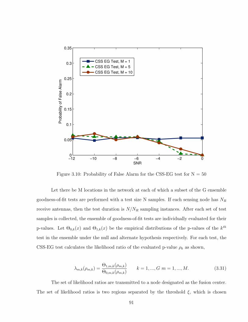
−12 −10 −8 −6 −4 −2 00
0.05
0.1
0.15
0.2
0.25
0.3
0.35
SNR
Pro
ba
bili
ty o
f F
als
e A
larm
CSS EG Test, M = 1
CSS EG Test, M = 5
CSS EG Test, M = 10
Figure 3.10: Probability of False Alarm for the CSS-EG test for N = 50
Let there be M locations in the network at each of which a subset of the G ensemble
goodness-of-fit tests are performed with a test size N samples. If each sensing node has NR
receive antennas, then the test duration is N/NR sampling instances. After each set of test
samples is collected, the ensemble of goodness-of-fit tests are individually evaluated for their
p-values. Let Θ0,k(x) and Θ1,k(x) be the empirical distributions of the p-values of the kth
test in the ensemble under the null and alternate hypothesis respectively. For each test, the
CSS-EG test calculates the likelihood ratio of the evaluated p-value ρk as shown,
λm,k(ρm,k) =Θ1,m,k(ρm,k)
Θ0,m,k(ρm,k)k = 1, ..., G m = 1, ...,M. (3.31)
The set of likelihood ratios are transmitted to a node designated as the fusion center.
The set of likelihood ratios is two regions separated by the threshold ξ, which is chosen
91

using the Neyman-Pearson criterion for a fixed area under the set of combined hypothesis
Θ0,k(x) for k = 1, ..., G. Note the important fact that through the use of Theorem 2, the p-
value distribution under the null hypothesis is known regardless of the size of the individual
EG tests and the distribution of the p-values under the alternate distribution. Thus, the
threshold can be set at the fusion center without the transfer of any side information from the
individual nodes. Consequently, the Collaborative Spatially separated Ensemble Goodness-
of-Fit Tests (CSS-EG) test operates with a high degree of flexibility in choosing the most
powerful test for a given set of test samples, and fully leverages the non-parametric nature
of goodness-of-fit procedures.
This test works extremely well in the situation where the sample size per test is
very small but the number of locations where such tests that are conducted is reasonably
large. The p-values under any test follow a fixed distribution under the two hypotheses. As
effective small sample testing for uniformity is possible, it is possible to use such a test to
robustly reach a decision. As we will show, the CSS-EG test works so well that it is to be
preferred unless its implementation is unfeasible. The downsides to using this test are 1)
the computational burden is higher, 2) the tuning of the test sample size and the threshold
settings is not obvious, although we provide sufficient guidelines.
3.7 Results
In this section, we present the improvement in the performance of the Φ-Divergence
based EG tests over the Kolmogorov-Smirnov test and the energy detector through simula-
tion results under diverse settings.
92

3.7.1 Simulation Scenario
We consider a setup that consists of a single primary user in a frequency flat fading
environment with a block transmission/reception of size T symbols per block. The primary
transmitter and the secondary receiver have 2 antennas each, i.e, NT , NR = 2. Thus the
test size is N = NR × T complex samples. Quadrature Phase Shift Keying modulation is
employed and the noise is circularly complex Gaussian with a spatial correlation coefficient
of 0.2 between the two antennas. At the initiation of the testing period in the absence
of the primary signal, a sequence of training samples is obtained with a duration of N =
100 complex samples. These training samples are used to estimate the distribution of the
test samples under the null hypothesis. This density estimation step is performed using a
Gaussian kernel as shown below. The bandwidth of the kernel is set to be 0.1 times the
bandwidth provided by the Sheather-Jones bandwidth estimation procedure. Such a setting
provides the correct smoothing of the density. In the case of the energy detector test, the
training samples are necessary to estimate the variance of the noise distribution.
3.7.1.1 Handling Complex Data
The goodness-of-fit tests have been defined over the support of real numbers R
whereas the baseband I-Q test samples are complex numbers C. One approach to apply
the goodness-of-fit tests to complex data is via the use of two dimensional KS tests [91–
93]. But, such tests impose a significant overhead in terms of the computational complexity
which is O(n3), or under simplifying assumptions, it reduces to O(n2). Also, the theory of
two dimensional tests has not yet been extended to GoF tests other than the Kolmogorov
Smirnov test. It has previously been proposed that amongst all the variants of the Kol-
mogorov Smirnov test, the 1-dimensional test that considers the magnitude of the received
samples provides the best performance [65]. Our simulations provided similar results for
the Φ-Divergence based goodness-of-fit tests for s ∈ (−1, 2), and we will only focus on the
93
relative performance of the tests that operate on the magnitudes of the received complex
samples.
After the training phase, each goodness-of-fit test statistic is evaluated using equation
(3.10). Also, the corresponding p-value is calculated using the distribution of the test statistic
that is approximated with high accuracy using the Noe recursion relations [78, 94]. Note that
the p-values can be pre-calculated and stored in look-up tables. Only the p-values are used
in later processing and act as the summary statistic. For individual goodness-of-fit tests, the
level of significance α for the test is decided a priori, that corresponds to the probability of
falsely rejecting the null hypothesis (PFA). If the p-value is less than α, the null hypothesis
is rejected. The energy detector test calculates the energy of the received samples as YYH
and compares it to a threshold given by
3.7.1.2 Test Power for individual Goodness-of-Fit test
The power of a statistical test is the measure of its discriminatory power under an
alternative hypothesis. We compare the powers of the Φ-Divergence based goodness of fit
test against the Kolmogorov Smirnov test using Monte Carlo methods. The figure shows the
distribution of the test statistics for 3 representative tests in the ensemble over 106 trials for
each hypothesis. The null hypothesis is, without loss of generalization, assumed to be an
uniform distribution. The alternate hypothesis is a chi-squared distribution followed by the
received statistic. These distributions are converted into the equivalent p-value distributions
using Theorem 1.
3.7.2 Ensemble Goodness-of Fit (EG) test based on Φ-Divergences
The EG test thresholds are implemented as per the algorithm described in Section
3.5.2 for the following specifications. The ensemble consists of 7 Φ-divergence tests in addi-
94

tion to the Kolmogorov-Smirnov test for values of s = −1,−0.5, 0, 0.5, 1, 1.5, 2. This ensemble
is found to comprehensively improve on the performance of each individual test, including
the Kolmogorov-Smirnov test, but is not the only possible configuration. Any number of
tests can be chosen to form the ensemble. The value of s = 0 gives maximum weight to
changes in central portion of the density function. And changing the value of s away from
0 gives increasing weight to changes in the tail areas of the density function. Also, the be-
havior of the phi-divergence is well characterized for any choice of s in the range [−1, 2] and
there is support for implementing this in the R statistical software package. While, we have
chosen s with a spacing of 0.5, a finer spacing will give better performance but also increase
the computational load. The performance of the Ensemble Goodness-of-Fit test is shown in
figure 3.8 for a test sample size of N = 50, i.e, the received block size T = 25. The level of
significance for Probability of False Alarm is set as α = 0.05 and the second order threshold
for Probability of Missed Detection is set to be β = 0.1 using the method described in Section
3.5.2. The p-value corresponding to β is calculated empirically for each SNR level and noise
distribution. The interim region is setup as the randomized testing region. Figure (3.8a) and
figure (3.8d) plot the PD and PFA performance in presence of Gaussian noise. The Signal-
to-Noise Ratio is varied from -12 dB to 0 dB. As the noise realization for the energy detector
follows the model exactly, its performance is better than that of the goodness-of-fit tests.
Also, the Ensemble Goodness-of-Fit test uniformly outperforms the Kolmogorov-Smirnov
test alone. This behavior is expected because of the rake like selectivity property of the
test mentioned in Section 3.5.2, and can be seen through all operating conditions. Thus,
the EG test is a consistent upper bound to the Kolmogorov-Smirnov test. Figure (3.8b)
and figure (3.8e) plot the PD and PFA performance in presence of Middleton Class A noise
mixture distribution. The Middleton noise has a Γ = 0.5 at both antennas and A = 0.2. Γ
controls the ratio of the Gaussian noise component to the Non-Gaussian noise component in
the mixture distribution. For such a mixture with a dominant Gaussian noise, the power of
95
the goodness-of-fit tests as measured by the PD is now better than that for Gaussian noise
alone, and matches that of the Energy detector at SNR > −4 dB. But, the critical point
to note here is that false alarm events, given by PFA, are significantly higher for the energy
detector. Thus the design parameters are violated for the ED test while the EG test and
the KS test still satisfy the PFA design constraints.
3.8 Conclusion
We have shown that nonparametric goodness-of-fit tests provide a robust solution to
the problem of severe degradation of the performance of parametric tests like the energy
detector. A systematic approach to design a nonparametric test suited to the particular set
of alternative hypothesis is proposed via using the Φ-divergence based goodness-of-fit tests.
These are are parameterized through s, and for all values of s, accurate procedures to calcu-
late the test tables exist. Also, the Ensemble Goodness-of-Fit test that comprises of these
Φ-divergence tests is shown through extensive simulations to consistently outperform the in-
dividual goodness-of-fit tests, including the Kolmogorov-Smirnov test. We have also derived
the Collaborative Spatially Separated EG method that leverages the unique properties of
the p-value summary metric to perform rapid distributed decision fusion.
96

Chapter 4
Sequential Approaches to Spectrum Sensing
4.1 Introduction
We have seen how Cognitive Radio (CR) provides an effective framework for oppor-
tunistic and efficient reuse of the scarce spectrum resources, e.g, [9], [13]. The process of
detection of spectral holes is the key enabler of Dynamic Spectrum Access (DSA) in cog-
nitive radio networks. A variety of methods for DSA have been proposed in the literature
such as energy detection, cyclostationarity based detection, eigenvalue based detection and
wide band spectrum sensing, see for example [95], [96]. These spectrum sensing methods
are classified into two categories: blind methods which work irrespective of the nature and
type of PU transmission and non-blind methods which exploit knowledge of the nature of
PU transmission. The energy detector is a blind method. It makes a decision based on the
estimate of the energy in the received signal. In contrast, non-blind techniques are based on
feature detection. Except for energy detection, these methods aim to deliver performance
improvement at the expense of significantly larger sensing times. We will focus on efficient
implementations of the Energy Detector (ED).
4.1.1 Related Work
The ED was recently popularized in the context of IEEE 802.22 Cognitive Radio
Networks [97]. These networks are required to detect the primary user at extremely low
Signal to Noise Ratios (SNRs) of upto -25db. Another constraint is the small upper limit
97
(on the order of milliseconds) on the sensing window. There exists a large body of work which
investigates the performance of the energy detector, e.g, [13], [98], [99] etc. As the structure
of the signal being detected is not known, matched filters cannot be implemented and energy
detectors are commonly used [100]. But, it has been shown that energy detector performance
degrades under lognormal shadowing [101, 102] though collaborative detection methods have
been proposed to improve the robustness of spectrum sensing to shadowing [103]. In this
chapter we investigate the behavior of spectrum sensing under sequential detection schemes.
A variety of distributed sequential detection methods based on information transfer between
the nodes, or between the node and a fusion center at each time step of the sequential
detection have been proposed for sensor networks [104]. For cognitive radios, extremely
reliable and fast detection of the primary user is critical which makes transfer of information
between the secondary users and the central node at each time step as assumed in these
works inviable. In contrast our approach proposes a hierarchical sequential detection scheme
wherein sequential detection of the classical kind is carried on at the level of secondary users
followed by a second level of sequential detection at the central node. The authors of this
work were amongst the first to implement a sequential approach to energy detection for
spectrum sensing [105], [106]. Other sequential based approaches have since been proposed
all of which have the goal of reducing the sensing time [107], [108], [109] but none of them
address the significant overhead reduction and performance gains achieved by hierarchical
tests that we study here.
4.1.2 Our Contributions
In this chapter we formulate a novel Sequential Energy Detector, characterize its per-
formance gains and demonstrate a throughput increase of 2 to 6 times over the Fixed Size
ED test as measured using the Relative Efficiency of the test. Also the issue of sensitivity
of the Sequential Test to primary signal variance estimation is addressed at length. Specif-
98

ically, we develop an Iterative Hybrid Bayesian method to robustly estimate the primary
signal variance.The rest of this chapter is organized as follows. In Section 4.2 we introduce
the assumptions. We review the conventional Fixed Sample Size (FSS) ED and the ba-
sic Sequential Test in Section 4.3. The novel SEquential Energy Detection (SEED) test is
introduced in Section 4.4 & the Iterative Hybrid Bayesian Update method in Section 4.5.
4.2 Notation and Assumptions
In this section we formulate the sequential detection problem. The channel is modeled
as per eqn. (4.1) for n = 1, . . . .
x(n) = hs(n) + v(n) : H1 & x(n) = v(n) : H0 (4.1)
Here, s(n) is the Primary User (PU) signal, v(n) is the Additive White Gaussian Noise
(A.W.G.N), x(n) is the signal received at the CR and h is the instantaneous channel gain.
Also, x = [x(1)x(2)...x(n)]. We make the following assumptions:
A.1 s(n) is independent identically distributed (i.i.d) zero mean circularly complex Gaussian
with variance σ2s . s(n) ∼ N (0 , σ2
s ).
A.2 v(n) is i.i.d zero mean circularly complex Gaussian with variance σ2v distributed as
∼ N (0 , σ2v ).
A.3 h is constant and normalized to unity throughout the test duration.
A.4 s(n) and v(n) are mutually independent.
A.5 Perfect knowledge of the noise variance σ2v at the CR end.
99

4.3 Review of ED and Sequential Detector
The sequential test is most naturally introduced as an extension of the FSS energy
detector. Here we will summarize the structure of the conventional ED as described in [110].
For the problem setting described above of an non deterministic signal in white Gaussian
noise, it is known that the energy detector is the optimal test [110]. The test is given as,
Decide H0 or H1 as λ(x) =f(x|H1)
f(x|H0)Q γ. (4.2)
λ(x) =
1
(2π(σ2s+σ2
v))N/2 exp(− 1
2(σ2s+σ2
v))∑N
n=1 |x(n)|2)
1
(2π(σ2v))N/2 exp
(− 1
2σ2v
∑Nn=1 |x(n)|2
) . (4.3)
λL(x) =N
2ln
(σ2s
σ2s + σ2
v
)+
1
2
σ2s
(σ2s + σ2
v)
N∑n=1
|x(n)|2. (4.4)
As the functional λ is monotonic, the log likelihood ratio is expressed as shown above.
The FSS ED takes the form as shown in eqn. (4.5). T (x) is the sum of Gaussian random
variables and obeys a χ2 distribution as in eqn. (4.6).
T (x) =N∑n=1
|x(n)|2 Q γ. (4.5)
T (x)
σ2s + σ2
v
∼ χ22N : H1 &
T (x)
σ2v
∼ χ22N : H0 (4.6)
It has been shown that the number of samples (N) required for a given PD and PFA
is ∝ SNR−2. Thus, the energy detector has the drawback that at SNRs 1, it requires
a large number of samples. We will show later that sequential tests reduce the expected
number of samples required to maintain the same PD and PFA as the ED by more than 50%.
100
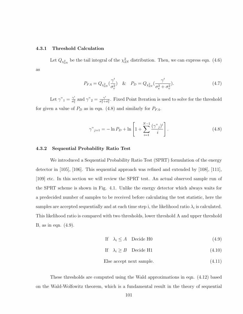
4.3.1 Threshold Calculation
Let Qχ22N
be the tail integral of the χ22N distribution. Then, we can express eqn. (4.6)
as
PFA = Qχ22N
(γ′
σ2v
) & PD = Qχ22N
(γ′
σ2s + σ2
v
). (4.7)
Let γ”1 = γ′
σ2v
and γ”2 = γ′
σ2s+σ2
v. Fixed Point Iteration is used to solve for the threshold
for given a value of PD as in eqn. (4.8) and similarly for PFA.
γ”j+1 = − lnPD + ln
[1 +
N−1∑i=1
(γ”j)i
i
]. (4.8)
4.3.2 Sequential Probability Ratio Test
We introduced a Sequential Probability Ratio Test (SPRT) formulation of the energy
detector in [105], [106]. This sequential approach was refined and extended by [108], [111],
[109] etc. In this section we will review the SPRT test. An actual observed sample run of
the SPRT scheme is shown in Fig. 4.1. Unlike the energy detector which always waits for
a predecided number of samples to be received before calculating the test statistic, here the
samples are accepted sequentially and at each time step i, the likelihood ratio λi is calculated.
This likelihood ratio is compared with two thresholds, lower threshold A and upper threshold
B, as in eqn. (4.9).
If λi ≤ A Decide H0 (4.9)
If λi ≥ B Decide H1 (4.10)
Else accept next sample. (4.11)
These thresholds are computed using the Wald approximations in eqn. (4.12) based
on the Wald-Wolfowitz theorem, which is a fundamental result in the theory of sequential
101
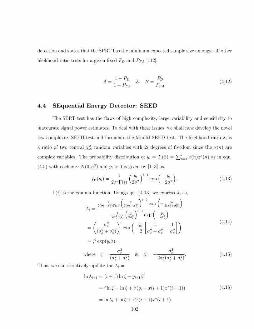
detection and states that the SPRT has the minimum expected sample size amongst all other
likelihood ratio tests for a given fixed PD and PFA [112].
A =1− PD1− PFA
& B =PDPFA
. (4.12)
4.4 SEquential Energy Detector: SEED
The SPRT test has the flaws of high complexity, large variability and sensitivity to
inaccurate signal power estimates. To deal with these issues, we shall now develop the novel
low complexity SEED test and formulate the Min-M SEED test. The likelihood ratio λi is
a ratio of two central χ22i random variables with 2i degrees of freedom since the x(n) are
complex variables. The probability distribution of yi = Ti(x) =∑i
n=1 x(n)x∗(n) as in eqn.
(4.5) with each x ∼ N(0, σ2) and yi > 0 is given by [113] as,
fY (yi) =1
2σ2Γ(i)
( yi2σ2
)i−1
exp(− yi
2σ2
). (4.13)
Γ(i) is the gamma function. Using eqn. (4.13) we express λi as,
λi =
12(σ2
s+σ2v)Γ(i)
(yi
2(σ2s+σ2
v)
)i−1
exp(− yi
2(σ2s+σ2
v)
)1
2σ2vΓ(i)
(yi
2σ2v
)i−1
exp(− yi
2σ2v
)=
(σ2v
(σ2s + σ2
v)
)iexp
(−yi
2
[1
σ2s + σ2
v
− 1
σ2v
])= ζ i exp(yiβ).
(4.14)
where ζ =σ2v
(σ2s + σ2
v)& β = − σ2
s
2σ2v(σ
2s + σ2
v). (4.15)
Thus, we can iteratively update the λi as
lnλi+1 = (i+ 1) ln ζ + yi+1β
= i ln ζ + ln ζ + β(yi + x(i+ 1)x∗(i+ 1))
= lnλi + ln ζ + βx(i+ 1)x∗(i+ 1).
(4.16)
102

0 5 10 15 20 25−0.5
0
0.5
1
1.5
2
2.5
Sample Length
Like
lihoo
d R
atio
(la
mbd
a)SNR = −3.8 dB N(ED)=20
LRA = 0,06B = 1.92
Figure 4.1: Sample Run of the Sequential Test Statistic
Eqn. (4.16) shows that the test statistic update term is linear in complexity as ln ζ and
β are constants. This formulation allows a natural simplification of the implementation of the
SEED test and avoids the approximations made by [109] and others. We use this iterative log
likelihood ratio update formula to reduce the computational complexity. The χ2 distribution
converges asymptotically to the Normal distribution as per the Central Limit Theorem.
The χ2 distribution is commonly approximated by the equivalent normal distribution for a
sample size greater than 20. Figure 4.2 plots the Kullback-Leibler distance between the χ2
distribution and its approximation. It is seen that the approximation is highly inaccurate
for N < 15. Also, our SEED test operates for the most part in this low sample region and
hence use of the normal approximation introduces large errors in analysis of sequential tests
which we avoid here.
103

0 5 10 15 20 25 300
100
200
300
400
500
600
700
800
900
Degree of Freedom of Chi Squared RV
Kul
lbac
k−Le
ible
r D
iver
genc
e
Asymptotic Convergence to Normality of Chi Squared Distribution
Figure 4.2: χ2 Distribution Approximation
4.4.1 SEED Performance Evaluation
The stopping time of a sequential test is a random variable. The relative performance
gain delivered by a sequential test can be succinctly characterized by comparing the expected
value of the sequential test duration to the fixed size of the energy detector. Let NSEED
be the Average Sample Number (ASN) of the sequential test and NED be the size of the
energy detector. The Relative Efficiency, η, of a sequential test over a fixed sample size test
is defined as the ratio of the expected sample size (i.e ASN) of the sequential test to the
sample size of the fixed sample size test with the same size and power.
η = NED/NSEED. (4.17)
The plots shown in Fig.4.3 for a fixed SNR were obtained as follows. For a given PD and
NED, the energy detector threshold γ” is found. Using the fixed point iteration in eqn.(4.8)
the corresponding PFA is calculated. Once we get the PFA and PD, we can construct the
104

(a)
(b)
(c)
Figure 4.3: Relative Efficiency of Seed vs ED for increasing PD with (a) -5 dB SNR (b) -3
dB SNR and (c) 3 dB SNR
105

equivalent SEED test and obtain the ASN using which the Relative Efficiency of the SEED
test is calculated. The plots show that at high PD values for low (negative) SNRs, η increases
as the size of corresponding ED test increases. But, in the high SNR domain, η decreases as
the size of ED test increases. This is because the fixed sample size ED test has very good
performance in the high SNR region and fares poorly in the low SNR operating region.
4.4.2 Problems with Wald Approximations and the Min-M SEED
The thresholds A and B are derived under the assumption that the test statistic
does not overshoot the threshold boundary at the sequential test stopping time. But this
condition usually doesn’t hold in practice and the design values of PFA and PD for the SEED
test are not obtained. We introduce a novel variation called the Min-M SEED test in which
a minimum of M samples are always collected before the test can terminate. This reduces
the effect of spurious values and brings the design values of PFA and PD in line with the
practically obtained values but the cost paid is a reduction in the relative efficiency of SEED
test. The plots in Fig.4.3 implement a Min-1 SEED while Fig.4.4 uses the standard SEED.
The higher variability and the higher efficiencies are easily noticed in Fig.4.4.
4.5 Signal Variance Estimation
Figures 4.3 and 4.4 demonstrate the significant throughput gain of the SEED test
over the FSS ED test and provide compelling evidence in favor of its widespread adoption.
However, there is an important drawback to the sequential testing methodology. In designing
the ED, we require only an accurate knowledge of the noise variance to calculate the ED
thresholds using eqn. (4.7) as its PD and PFA are interdependent. By contrast, in the SEED
test, we need perfect knowledge of both the primary signal power and the noise variance to
setup the test thresholds. In practice, the primary user signal is assumed to be completely
106

Figure 4.4: SNR vs η for a Pd = 0.95
unknown. Moreover, we have at most approximate estimates of the distance from the PU
transmitter, the propagation loss factor and the channel gain. These constraints introduce
high variability in the signal power estimates at the CR.
4.5.1 Sensitivity to Signal Variance Estimate
Eqn. (4.13) shows the dependence of λi on the signal variance σ2s and can be used
to calculate the sensitivity of the likelihood ratio to the estimated σ2s . Unfortunately, this
dependence is not amenable to analysis and is demonstrated here via simulations. Fig. 4.5
plots the percentage change in the efficiency of the SEED test as increasing error is introduced
in the estimate of signal power σ2s . There is a performance degradation of almost 15% for a
30% estimation error.
107
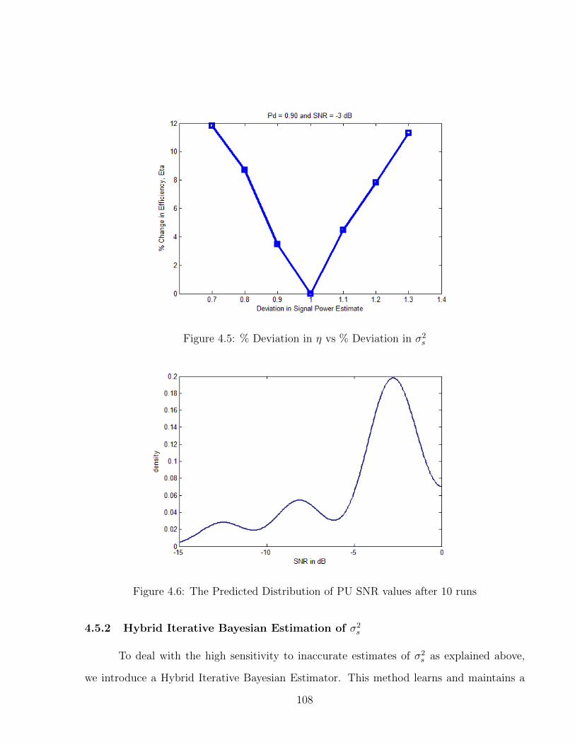
Figure 4.5: % Deviation in η vs % Deviation in σ2s
Figure 4.6: The Predicted Distribution of PU SNR values after 10 runs
4.5.2 Hybrid Iterative Bayesian Estimation of σ2s
To deal with the high sensitivity to inaccurate estimates of σ2s as explained above,
we introduce a Hybrid Iterative Bayesian Estimator. This method learns and maintains a
108

distribution for σ2s . This prior distribution is used to estimate the future value of the signal
energy and the estimate is refined as more and more samples are collected. Before we explain
the method in detail, we note that the signal variance has to be estimated from the sporadic
small intervals when a detection event occurs. In contrast, the problem of noise variance
estimation has been extensively studied, see for e.g [114], and accurate estimates can be
obtained by out-of-band sensing. We assume perfect knowledge of noise variance in order to
isolate the effects of signal variance on the SEED test.
4.5.2.1 Initialization
The instantaneous value of σ2s depends on the shadowing and fading of the channel.
Also, Fig. 4.3 shows that the efficiency of the test improves with SNR and the IEEE 802.22
standard has stringent specifications for detection of low power TV signals in the negative
SNR region. Considering these factors, the σ2s estimator is initialized conservatively using
a uniform distribution over [-20dB, 0dB] as the informative prior. Once the prior has been
initialized, it will be updated every time the SEED algorithm produces a detection event.
4.5.2.2 Update
As the SEED test progresses, it will produce detection events. From the channel
model, σ2x = σ2
s + σ2v . Thus the estimator of the signal variance is σ2
s,old = σ2x − σ2
v . The
updated posterior distribution f(x) is obtained via adding a Gaussian kernel centered at
the obtained σ2s . We implement this as a Kernel Density Estimator with a Gaussian Ker-
nel. f(x) =∑N
i=1K(x,Xi, t) where K(x,Xi, t) = 1√2πt
exp (− (x−Xi)2
2t). t is the estimator
bandwidth selected by the data-dependent Sheather-Jones method [115], [116]. Thus, the
posterior distribution tends towards a Mixture of Gaussian formulation. We use a unique
variation in which the older kernels are assigned exponentially decreasing weights to account
for the time varying received signal power.
109

Table 4.1: Performance of SNR Prediction in 10 Iterations
SNR Mean Predicted SNR % Deviation in η
-3.0dB -4.2 3.6
-10.0dB -9.2 5.4
-15.0dB -17.1 6.9
4.5.2.3 Prediction
A sample drawn probabilistically from the updated posterior distribution is the pre-
dicted value of the signal power σ2s,new and is used to initialize the next iteration of the
SEED test. This probabilistic approach as opposed to the use of the mean of the posterior
increases the robustness of the estimation procedure and helps avoid local attractor points.
The efficiency error reduction through the prediction performance is shown in Table 4.1 .
4.6 Distributed Sequential Detection
In Section 4.4 we have formulated the sequential SED test that runs at an individual
CR node. A typical CR has a single antenna which can be used for either sensing or
transmitting and the secondary transmissions prevent other CRs from detecting PU signals.
The necessity for spectrum sensing to be interleaved with secondary transmission has led
to the adoption of a Quiet Period (QP). The QP is a synchronized time interval when all
secondary transmissions cease. We have seen in the last section that Sequential Tests are
uniquely suited for Cognitive Radio Networks which need to minimize sensing overhead while
attaining a specified detection performance. There is a need to adopt a holistic approach
to the goal of minimization of sensing overhead. Let dk = 0, 1 be the decision of the kth
110

CR whose SED terminates at time Tk. Also, TBS is the DSED termination time at the base
station and is the system sensing overhead. At one end is the policy where the base station
simply decides the same as the first CR to report. We show in Section 4.8 that such a ’one
shot’ strategy has very poor performance in terms of PFA. At the other end is the policy
where the base station waits for all CRs to terminate their SED tests and report before it
decides. But this can take a very long time in the worst case as the termination time of
the SED is a random variable. Assuming all CRs stop sensing at TBS, the system sensing
overhead is bounded as mink∈[1,N ] Tk < TBS < maxk∈[1,N ] Tk. There exists a tradeoff between
the two extreme sensing strategies which can be formulated as shown below.
minTBS s.t PD > PD,target & PFA < PFA,target. (4.18)
4.6.1 Doubly Sequential Energy Detection (DSED)
The novel Doubly Sequential Energy Detection (DSED) test that we propose here
minimizes the sensing overhead while maintaining the target PFA and PD. In the DSED
test, a sequential SED test runs at each CR node and a variable time is required by the
Base Station to reach a final decision. It does not stop sensing when the first CR reaches
a decision. Instead, sensing is continued till more and more CRs terminate and sufficient
data is available to the base station to be able to reach a decision with a pre-fixed certainty.
Thus, the base station can be interpreted as running a second sequential test. We shall call
this unique structure a Doubly Sequential Test.
The termination time of the sequential test is a random variable. Unfortunately, an
exhaustive mathematical formulation of the Doubly Sequential structure is intractable. In
this section we will mainly characterize the DSED performance through simulations and
provide supporting theoretical results where possible. Let Z = log f1(y)f0(y)
. In the SED, y =
T (x) =∑M
n=1 |x(n)|2. Wald has derived the following lower bounds for the expectation of
111
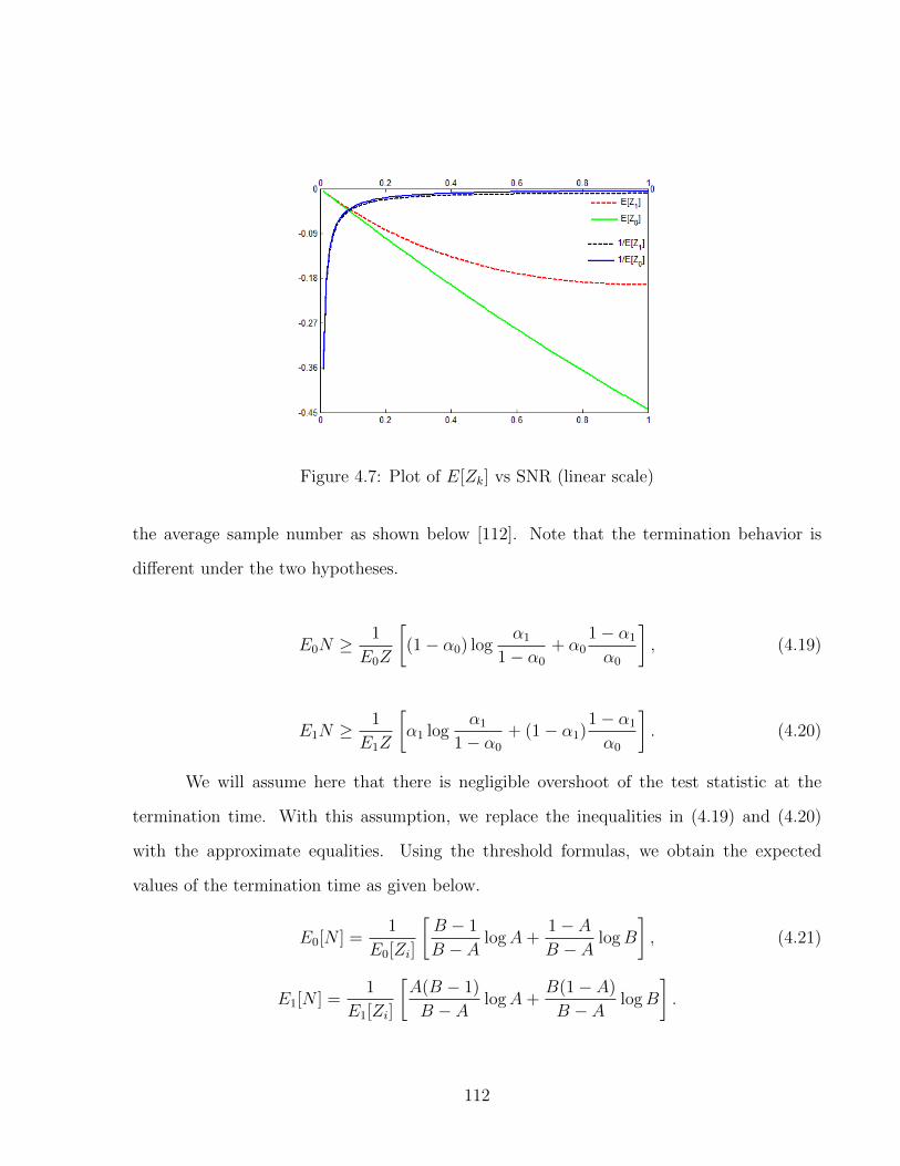
Figure 4.7: Plot of E[Zk] vs SNR (linear scale)
the average sample number as shown below [112]. Note that the termination behavior is
different under the two hypotheses.
E0N ≥1
E0Z
[(1− α0) log
α1
1− α0
+ α01− α1
α0
], (4.19)
E1N ≥1
E1Z
[α1 log
α1
1− α0
+ (1− α1)1− α1
α0
]. (4.20)
We will assume here that there is negligible overshoot of the test statistic at the
termination time. With this assumption, we replace the inequalities in (4.19) and (4.20)
with the approximate equalities. Using the threshold formulas, we obtain the expected
values of the termination time as given below.
E0[N ] =1
E0[Zi]
[B − 1
B − AlogA+
1− AB − A
logB
], (4.21)
E1[N ] =1
E1[Zi]
[A(B − 1)
B − AlogA+
B(1− A)
B − AlogB
].
112

Using (4.14) the Log Likelihood Ratio Z of the SED test becomes Z =∑i
k=1 Zi, i.e,
a sum of i.i.d statistics Zi,
Zi = ln ζ + βx(i+ 1)x∗(i+ 1). (4.22)
Taking the expectation of (4.22), with k = 0 , 1 corresponding to the hypothesis H0 and H1
respectively,
Ek[Z] = E [log ζ + yiβ] = log ζ + σ2xβ. (4.23)
After further simplification with σ2x = σ2
s +σ2v for H1 and σ2
x = σ2v for H0, we get the following
relations.
E0[Zi] = −log(1 + γ) +γ
2(1 + γ): H0
E1[Zi] = −log(1 + γ) + 2γ : H1 (4.24)
Equations (4.21) and (4.24) shown that the distribution of the termination time depends
on the PD, the PFA and the SNR of the system. The behavior of Ek[Zi] for SNR γ < 1
is plotted in Figure 4.7. We note that for γ < 0.1, i.e, γ < − 10 dB, the SED stopping
time significantly deteriorates for a fixed PD and PFA. This behavior has two important
consequences. 1) The SED is a truncated sequential test and is forced to stop and reach
a decision after the maximum sensing duration. As the SNR decreases, the test reaches
truncation more often and the delivered PD suffers as seen in Figure 4.8. 2) When shadowing
is taken into consideration, there is a spread observed in the SNRs. This means that the
earliest CRs to terminate are highly likely to be the ones that have an extreme value of the
SNR and this behavior is exploited in the Distributed SED. In the next section we present
strategies for the termination of the DSED at the Base Station.
113

4.7 Termination Criteria at Base Station
4.7.1 One Shot Detection
This is the simplest strategy where the base station terminates the DSED when the
first CR terminates and communicates its decision, i.e, TBS = T1, i.e, the base station reaches
a final decision in a one-shot manner. While this is an effective strategy for the scenario of
i.i.d observations at each CR, the system performance is severely degraded under log-normal
shadowing. The degradation occurs because the overall system performance is dictated by
the earliest CR to reach a decision, which is often the one that also experiences a false alarm
due to extreme value of γ as explained in the last section. The simulation results verify that
the the sensing time is reduced but detection performance severely degrades.
4.7.2 First-M-Positive Detection
In First-M-Positive Detection, the Base Station continues the DSED test till it has
received M decisions in favor of a particular hypothesis. The test then terminates and
that particular hypothesis is the DSED decision. Heuristically, we found that setting M ≥
4 delivers good performance. We observe that this choice of M depends only upon the
shadowing present and does not scale with the number of nodes in the secondary network.
This strategy exploits the lower stopping times at high SNRs as in Fig. 4.7 to terminate
faster while at the same time it increases the robustness against extreme shadowing values.
TBS = arg mink
(k∑i=1
1[di=1] = M
)∧
(k∑i=1
1[di=0] = M
).
4.7.3 Wait-Till-TTh Detection
The Base Station waits till it receives the first decision after a duration TTh has
passed. The final decision is made in favor of the majority of individual CR decisions. Here,
114
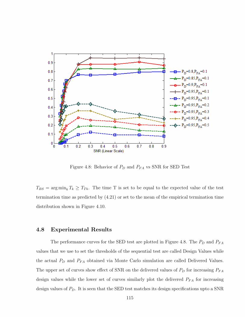
Figure 4.8: Behavior of PD and PFA vs SNR for SED Test
TBS = arg mink Tk ≥ TTh. The time T is set to be equal to the expected value of the test
termination time as predicted by (4.21) or set to the mean of the empirical termination time
distribution shown in Figure 4.10.
4.8 Experimental Results
The performance curves for the SED test are plotted in Figure 4.8. The PD and PFA
values that we use to set the thresholds of the sequential test are called Design Values while
the actual PD and PFA obtained via Monte Carlo simulation are called Delivered Values.
The upper set of curves show effect of SNR on the delivered values of PD for increasing PFA
design values while the lower set of curves similarly plot the delivered PFA for increasing
design values of PD. It is seen that the SED test matches its design specifications upto a SNR
115
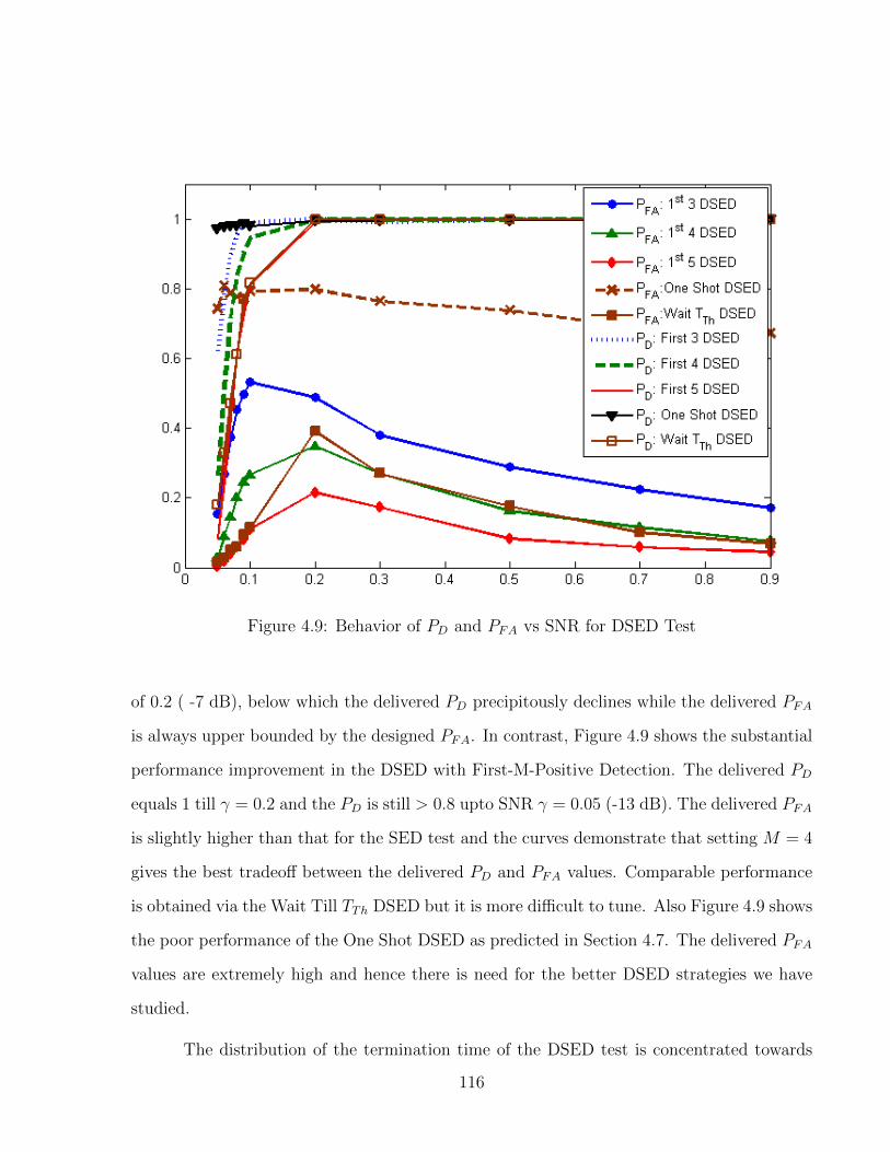
Figure 4.9: Behavior of PD and PFA vs SNR for DSED Test
of 0.2 ( -7 dB), below which the delivered PD precipitously declines while the delivered PFA
is always upper bounded by the designed PFA. In contrast, Figure 4.9 shows the substantial
performance improvement in the DSED with First-M-Positive Detection. The delivered PD
equals 1 till γ = 0.2 and the PD is still > 0.8 upto SNR γ = 0.05 (-13 dB). The delivered PFA
is slightly higher than that for the SED test and the curves demonstrate that setting M = 4
gives the best tradeoff between the delivered PD and PFA values. Comparable performance
is obtained via the Wait Till TTh DSED but it is more difficult to tune. Also Figure 4.9 shows
the poor performance of the One Shot DSED as predicted in Section 4.7. The delivered PFA
values are extremely high and hence there is need for the better DSED strategies we have
studied.
The distribution of the termination time of the DSED test is concentrated towards
116
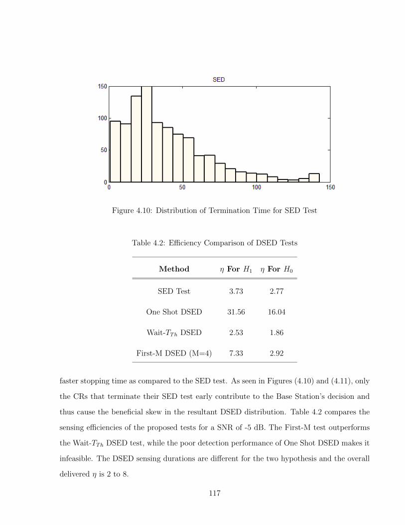
Figure 4.10: Distribution of Termination Time for SED Test
Table 4.2: Efficiency Comparison of DSED Tests
Method η For H1 η For H0
SED Test 3.73 2.77
One Shot DSED 31.56 16.04
Wait-TTh DSED 2.53 1.86
First-M DSED (M=4) 7.33 2.92
faster stopping time as compared to the SED test. As seen in Figures (4.10) and (4.11), only
the CRs that terminate their SED test early contribute to the Base Station’s decision and
thus cause the beneficial skew in the resultant DSED distribution. Table 4.2 compares the
sensing efficiencies of the proposed tests for a SNR of -5 dB. The First-M test outperforms
the Wait-TTh DSED test, while the poor detection performance of One Shot DSED makes it
infeasible. The DSED sensing durations are different for the two hypothesis and the overall
delivered η is 2 to 8.
117

Figure 4.11: Distribution of Termination Time for DSED Test
4.9 Case Study 1- Sequential Sensing applied to the IEEE 802.22
Standard
The IEEE 802.22 Standard is the first practical implementation of the cognitive radio
technology [97, 117]. It is based on dynamic spectrum sensing and opportunistic access of the
bands that are not currently in use by TV transmitters. It exploits the fact that the average
TV market in the United States uses around 7 of the allotted 67 high power channels. FFT
based pilot sensing of the TV signal is recommended in the standard. The sensing is carried
out by averaging over a fixed number of multiple dwells (6-10). We propose a sequential
version of the scheme where the number of dwells required is dynamically varying according
to the fidelity of the received signal. We show via simulation that the proposed sequential
sensing strategy yields a throughput gain and reduces system overhead
118

4.9.1 FFT based Pilot Detection of ATSC signals
The FFT based pilot sensing method is a non-blind technique which meets the sensing
requirements of the 802.22 draft standard [118]. It uses the pilot present in ATSC DTV
signals. The ATSC signal has an 8-VSB (Vestigial Side Band) modulation with signal levels
of (-7,-5,-3,-1, 1, 3, 5, 7). For efficient carrier recovery at the receiving end, a pilot is added
to the signal through a DC offset of 1.25. In this section, we will focus only on ATSC signals.
The pilot is transmitted at a much higher SNR than the rest of the ATSC TV signal. This is
the main advantage of sensing only the pilot, as we can operate at a more favorable point on
the operating characteristics curve of the energy detector. We take the FFT of the captured
signal over a period of 1 ms or 5 ms, called a dwell. The power in the signal at a particular
frequency (say, the pilot frequency) is estimated as the square of the corresponding frequency
bin in its FFT. It can be easily shown that the pilot power follows a Chi-squared distribution
with 2 degrees of freedom. The hypothesis testing problem is to decide between a central
Chi Square and a non-central Chi square distribution with a non centrality parameter equal
to the SNR at the pilot frequency.
H0 ∼ χ22(0) (4.25)
H1 ∼ χ22(λpilot) (4.26)
The test reduces to comparing the power in the bin corresponding to the pilot fre-
quency to a threshold. The threshold is calculated using the Neyman-Pearson theorem to
meet the required values for the probability of missed detection (PMD) and probability of
false alarm (PFA). Calculation of the threshold requires the knowledge/estimation of the
SNR at the pilot frequency, as do all energy detectors. We assume that a perfect estimate
of the SNR is available for deriving the tests. The effect of uncertainty in knowledge of the
SNR is neglected. If the signal is in a deep fade or is very weak, a single dwell may give
119

erroneous results. Multiple dwells have to be used in practical implementations to improve
the detection performance [119].
4.9.2 Sequential Sensing of ATSC Pilot
In the multiple-dwell implementation of pilot sensing, the number of dwells is fixed a
priori, usually between 6 -10. We will now formulate a sequential implementation of the pilot
sensing scheme, where depending upon the uncertainty of the decision, a variable number
of dwells will be required. We will develop the sequential pilot sensing method in a similar
manner to our development of the SED test in last section. The sequential probability ratio
test (SPRT) allows us to arbitrarily specify the PMD and PFA we would like the system
to operate at, by the virtue of the variable run length of the test. We keep accepting new
samples till we can make a decision with a satisfactory certainty. The performance of a SPRT
is measured in terms of the average sample number (the average number of dwells) required.
At each iteration of the sequential test, we update the likelihood ratio, which is a function
of all the samples received within that time. The updated likelihood ratio is compared with
upper and lower thresholds. If either threshold is exceeded, we stop the test and reach a
decision. Otherwise we accept more samples till we are in a position to decide. Also,the
Walds approximations give us the thresholds.
4.9.2.1 Preprocessing of ATSC signal captures
The ATSC signal has a bandwidth of 6 MHz and the pilot is at the lower edge of
the band as shown in Figure 4.12. The IEEE 802.22 standard prescribes a database of
12 ATSC signal captures under varying real world multi-path fading, frequency offsets and
other distortions. The signal is sampled at 21.52 Msamples/sec and down converted to a low
central IF of 5.38 MHz (one fourth the sampling rate). An 8 MHz bandwidth IF filter was
used when capturing the signals.
120

Figure 4.12: Spectral Density of an ATSC channel
We follow the 802.22 standard recommended steps (1-4) [120] and then implement
our proposed sequential test.
A.1 Filter the signal using a passband filter with a 6 MHz bandwidth with a center fre-
quency of fIF = 5.38MHz. The filter is a brick wall filter.
A.2 Add the filtered noise and the scaled and filtered signal.
A.3 Estimate pilot frequency as the peak in the FFT nearest to the nominal pilot frequency
of 2.69MHz.
A.4 We need prior knowledge of the pilot power, the noise power at the pilot frequency
and the pilot SNR to run the test. We will estimate them by averaging over a large
number of realizations of the signal.
121
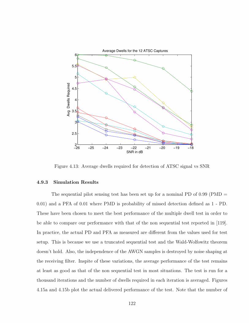
−26 −25 −24 −23 −22 −21 −20 −19 −182
2.5
3
3.5
4
4.5
5
5.5
6
SNR in dB
Avg
D
we
lls R
eq
uire
d
Average Dwells for the 12 ATSC Captures
Figure 4.13: Average dwells required for detection of ATSC signal vs SNR
4.9.3 Simulation Results
The sequential pilot sensing test has been set up for a nominal PD of 0.99 (PMD =
0.01) and a PFA of 0.01 where PMD is probability of missed detection defined as 1 - PD.
These have been chosen to meet the best performance of the multiple dwell test in order to
be able to compare our performance with that of the non sequential test reported in [119].
In practice, the actual PD and PFA as measured are different from the values used for test
setup. This is because we use a truncated sequential test and the Wald-Wolfowitz theorem
doesn’t hold. Also, the independence of the AWGN samples is destroyed by noise shaping at
the receiving filter. Inspite of these variations, the average performance of the test remains
at least as good as that of the non sequential test in most situations. The test is run for a
thousand iterations and the number of dwells required in each iteration is averaged. Figures
4.15a and 4.15b plot the actual delivered performance of the test. Note that the number of
122

−26 −25 −24 −23 −22 −21 −20 −19 −182
2.5
3
3.5
4
4.5
5
5.5
6
SNR in dB
Avg
D
we
lls R
eq
uire
d
Average Dwells for the 12 ATSC Captures
Figure 4.14: Distribution of the dwells required for sensing
dwells required is not constant but varies dynamically. Note also that the proposed sequential
test outperforms the fixed sample size test and yields a lower probability of missed detection.
We have set up the test to run for a minimum of two dwells. The average dwell number
increases as the SNR is decreased from -18 dB to -26 dB. Figure 4.13 shows the average
number of dwells required over the range of SNRs for sequential pilot detection. Also, the
spread of the dwells is plotted in the histogram for a SNR of -26 dB is plotted in Figure 4.14.
4.10 Conclusion
In this chapter we proposed a novel sequential energy detector (SED) which deliv-
ers significant reduction in sensing time as compared to the conventional fixed sample size
energy detector. We also formulated a Doubly Sequential Test (DSED) as a distributed ver-
sion of the SED test and characterized its performance. It was demonstrated that the DSED
123

−26 −25 −22 −20 −1810
−3
10−2
10−1
100
SNR in dB
PM
D
WAS−3−27−06022
WAS−51−35−05242
3WAS−311−36−06052
WAS−311−48−06052
WAS−68−36−05232
WAS−49−34−06142
WAS−311−35−06052
WAS−06−34−06092
WAS−49−39−06142
WAS−47−48−06132
WAS−32−48−06012
WAS−86−48−01722
(a)
−26 −24 −22 −20 −1810
−3
10−2
10−1
100
SNR in dB
PF
A
WAS−3−27−06022
WAS−51−35−05242
3WAS−311−36−06052
WAS−311−48−06052
WAS−68−36−05232
WAS−49−34−06142
WAS−311−35−06052
WAS−06−34−06092
WAS−49−39−06142
WAS−47−48−06132
WAS−32−48−06012
WAS−86−48−07122
(b)
Figure 4.15: The behavior with respect to SNR for (a) delivered probability of missed de-
tection PMD and (b) the delivered probability of false alarm PFA
124
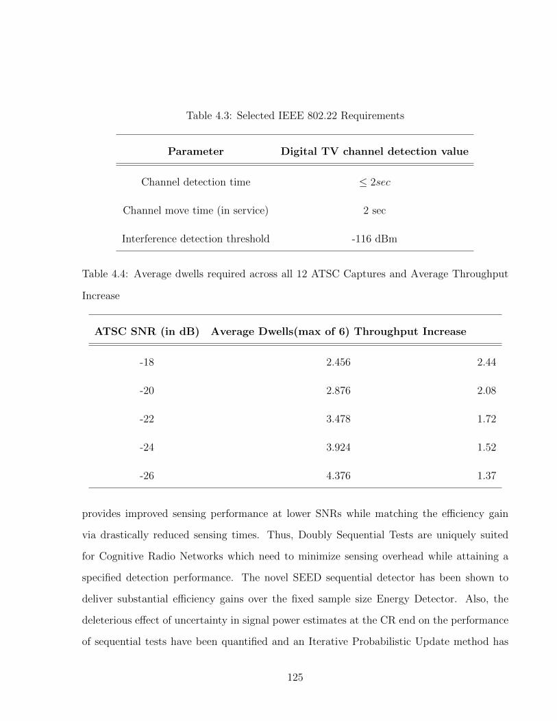
Table 4.3: Selected IEEE 802.22 Requirements
Parameter Digital TV channel detection value
Channel detection time ≤ 2sec
Channel move time (in service) 2 sec
Interference detection threshold -116 dBm
Table 4.4: Average dwells required across all 12 ATSC Captures and Average Throughput
Increase
ATSC SNR (in dB) Average Dwells(max of 6) Throughput Increase
-18 2.456 2.44
-20 2.876 2.08
-22 3.478 1.72
-24 3.924 1.52
-26 4.376 1.37
provides improved sensing performance at lower SNRs while matching the efficiency gain
via drastically reduced sensing times. Thus, Doubly Sequential Tests are uniquely suited
for Cognitive Radio Networks which need to minimize sensing overhead while attaining a
specified detection performance. The novel SEED sequential detector has been shown to
deliver substantial efficiency gains over the fixed sample size Energy Detector. Also, the
deleterious effect of uncertainty in signal power estimates at the CR end on the performance
of sequential tests have been quantified and an Iterative Probabilistic Update method has
125

been developed to robustly estimate the variance and thus improve the SEED test perfor-
mance. The superior performance of the family of sequential energy detectors has been
comprehensively studied from the perspective of Dynamic Spectrum Access applications.
126

Chapter 5
Conclusion
In this thesis we have presented various techniques for sensing and accessing the
latent capacity in wireless channels. We will now briefly revisit the salient points of these
techniques, elaborate on how the techniques fit into a comprehensive network sensing and
access framework, and point out avenues for expanding on our contributions within and
beyond the scope of cognitive radios.
Conventional Opportunistic Spectrum Access methodologies seek out opportunities
for the unlicensed secondary transmissions at the physical layer. The current models such as
white space, interference temperature limits and others are examples of this physical layer
based outlook towards cognitive radios. In Chapter 2 we introduced a novel transmission op-
portunity sensing paradigm which senses the opportunities at the MAC layer of the primary
network in contrast to most previous work. We developed a suite of transmit opportunity
detection methods that effectively exploit the gray space present in high traffic packet net-
works. Our methods adopted a holistic view of the primary network and could proactively
decide the maximum safe transmit power that does not affect the nodes in the primary net-
work. This was achieved via an implicit feedback mechanism from the Primary network to
the Secondary network. This is the first time that such a Primary User - Secondary User
feedback link has been shown to naturally arise in the framework of Opportunistic Spectrum
Access. This was achieved in part via use of primary network packet statistics such as packet
lengths and interarrival durations to rapidly and robustly perform change detection in the
127

primary network’s Quality of Service. Our field testing of these methods on real world de-
ployments of IEEE 802.11 campus wireless LANs demonstrate the potential of this approach
towards Opportunistic Spectrum Access.
In Chapter 3 we focused on the problem of detecting the presence or absence of a
licensed user on a specific channel. We addressed the more complex spectrum sensing setup
where the noise statistics are either completely arbitrary or a mixture of Gaussian and im-
pulsive noise. It has long been known that uncertainty in estimation of noise statistics, time
variability of the noise statistics or presence of significant non Gaussian interferers drastically
deteriorates the presence of conventional white space sensing methods. We demonstrated
here that using a nonparametric formulation delivers superior performance gains over the
more popular parametric spectrum sensing tests. The unique aspect of this work was our
use of goodness of fit tests for the purpose of inference in a non-parametric setting. We
provided the first comprehensive framework for decision fusion of an ensemble of goodness-
of-fit testing procedures through an Ensemble Goodness-of-Fit test. Also, for the first time
we introduced a generalized family of functionals and kernels called Φ-divergences which
allow us to formulate goodness-of-fit tests that are parameterized by a single parameter.
The performance of these tests is simulated under Gaussian and non-Gaussian noise in a
MIMO setting. We show that under uncertainty in the noise statistics or non-Gaussianity
in the noise, the performance of non-parametric tests in general, and phi-divergence based
goodness-of-fit tests in particular, is significantly superior to that of the energy detector with
reduced implementation complexity. In particular, the false alarm rates of our proposed tests
is maintained at a fixed level over a wide variation in the channel noise distributions. Addi-
tionally, we proposed a new and effective collaborative spatially separated version of the test
for robust combining of tests in a distributed spectrum sensing setting via use of p-values of
the test statistics and quantified the significant collaboration gains achieved.
It is critically important during spectrum sensing to detect the presence of the primary
128

user as rapidly as possibly so as to be able to vacate the channel and minimize the interference
caused to the licensed channel users. With this goal in mind, in Chapter 4 we developed the
sequential energy detection problem in the context of spectrum sensing for cognitive radio
networks. We formulated a novel Sequential Energy Detector and provide a comprehensive
study of its performance. Also, the sensitivity of such Sequential Test procedures to errors
in primary signal energy estimation is uniquely addressed in this work. Through simulations
it was demonstrated that our Sequential version of the energy detector delivers a significant
throughput improvement of 2 to 6 times over the fixed sample size test while maintaining
equivalent operating characteristics as measured by the Probabilities of Detection and False
Alarm. We applied our sequential energy detection test to demonstrate the throughput gains
for a case study of sensing real world capture of ATSC television signals under adverse channel
conditions within the framework of the IEEE 802.22 standard via the FFT based pilot energy
sensing technique. Finally, we further extended the sequential testing framework to a doubly
hierarchical setting with each CR performing sequential detection and the fusion center
performing a second tier of hard sequential test on the sequentially transmitted decisions of
these individual nodes.
There is an overarching themes common to the three principal contributions summa-
rized above. The real world wireless channel is a complex messy entity. It is erroneously over-
simplified for ease of analysis and for elegance of the theoretical formulations thus achieved.
Dealing with this real world complexity and nonidealities requires that the researcher be
prepared to go beyond his/her toy models. To give a specific example, most modeling in
cognitive radios assumes that the background noise is additive, white and Gaussian. In prac-
tice, only the thermal noise follows those properties, and in addition to thermal noise, there is
a significance presence of other noise such as front end non-linearities, spikes due to engines,
leakage from microwave ovens, cross channel interference and narrowband interference from
Bluetooth, wireless sensors and other low power pervasive communication devices, natural
129

sources such as lightning etc. Also, even the distribution of the AWGN noise can only be
imperfectly estimated and such imperfect estimation bounds the performance of spectrum
sensing methods like the energy detector. In a blind sensing environment as is typical in
cognitive radio settings, we cannot even assume to know the power statistics of the primary
users unless we tailor the cognitive radio to learn each type of primary transmission at each
frequency band of interest, which is a task of high magnitude of complexity. Summing up,
the tidy little parametric models of the signals of the primary users and background noise
statistics are almost always not usable in the real world, and the parameters are seldom
known to us exactly, as is required to tune those models. In our work, we recommend a shift
in perspective towards nonparametric modeling of Opportunistic Spectrum Access scenarios.
Such nonparametric models are perfectly suited for use when the probability distributions
are known with uncertainty, varying slowly over time or completely arbitrary.
Finally, we conclude by pointing out that the paradigm of Opportunistic Spectrum
Access is only the first tentative step towards the vision of a world of intelligent and flexibly
reconfigurable radios that seamlessly roam over the entire frequency band and integrate
into a single universal wireless network. Cognitive radios built on a foundation of advanced
Software Defined Radio technology show tremendous potential to achieve this goal. Today
the wireless world is divided into hundreds of distinct principalities and fiefdoms, with each
ruled by a combination of particular wireless technology, standard and intellectual property
strongholds. A state of such fragmentation coupled with a regulatory reluctance to overhaul
the spectrum policies and the potent inertia of the vested interests of legacy technologies are
formidable obstacles to a seamless and borderless wireless future. It is the fervent hope of the
authors that the new generation of smart Cognitive Radios and the associated technology
policies and standards will help us achieve the holy grail of a truly universal communications
network.
130

Appendices
131

Appendix A
Abbreviations
ACK Acknowledgment
AD Anderson Darling test
AIMSE Asymptotic Integrated Mean Square Error
ATSC Advanced Television Systems Committee
AMC Adaptive Modulation and Coding
BER Bit Error Rate
BPSK Binary Phase Shift Keying
CAP Channel Capture
CDF Cumulative Distribution Function
CR Cognitive Radio.
CRN Cognitive Radio Network
CSS-EG Collaborative Spatially Separated EG test
CTS Clear To Send
CvM Cramer von Mises test
132

DSA Dynamic Spectrum Access
DSED Doubly Sequential Energy Detection
DTV Digital Television
ED Energy Detector
EG Ensemble Goodness-of-Fit test
e.d.f Empirical Distribution Function
ETSI The European Telecommunications Standards Institute
FCC Federal Communications Commission
FFT Fast Fourier Transform
FSS Fixed Sample Size test
GoF Goodness of Fit
IT Interference Temperature
KDE Kernel Density Estimation
KL Kullback Leibler divergence
KS Kolmogorov Smirnov test
MAC Medium Access Control
MIMO Multiple Input Multiple Output
OFCOM Office of Communications
OSA Opportunistic Spectrum Access
133
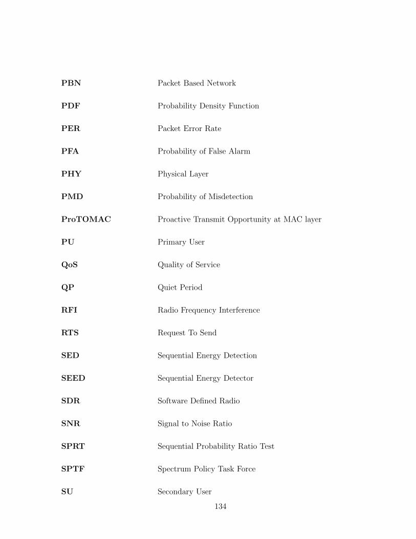
PBN Packet Based Network
PDF Probability Density Function
PER Packet Error Rate
PFA Probability of False Alarm
PHY Physical Layer
PMD Probability of Misdetection
ProTOMAC Proactive Transmit Opportunity at MAC layer
PU Primary User
QoS Quality of Service
QP Quiet Period
RFI Radio Frequency Interference
RTS Request To Send
SED Sequential Energy Detection
SEED Sequential Energy Detector
SDR Software Defined Radio
SNR Signal to Noise Ratio
SPRT Sequential Probability Ratio Test
SPTF Spectrum Policy Task Force
SU Secondary User
134

TEV Thresholded Extreme Value test
TM Transmit Margin
USRP Universal Software Radio Peripheral
WRAN Wireless Regional Area Network
WLAN Wireless Local Area Network
135

Bibliography
[1] V. Valenta, R. Marsalek, G. Baudoin, M. Villegas, M. Suarez, and F. Robert, “Survey
on spectrum utilization in europe: Measurements, analyses and observations,” pp. 1–5,
2010.
[2] M. McHenry, P. Tenhula, D. McCloskey, D. Roberson, and C. Hood, “Chicago spec-
trum occupancy measurements & analysis and a long-term studies proposal,” p. 1,
2006.
[3] M. Islam, C. Koh, S. Oh, X. Qing, Y. Lai, C. Wang, Y. Liang, B. Toh, F. Chin, G. Tan
et al., “Spectrum survey in singapore: Occupancy measurements and analyses,” pp.
1–7, 2008.
[4] S. Pagadarai and A. Wyglinski, “A quantitative assessment of wireless spectrum mea-
surements for dynamic spectrum access,” in Cognitive Radio Oriented Wireless Net-
works and Communications, 2009. CROWNCOM’09. 4th International Conference
on. IEEE, 2009, pp. 1–5.
[5] J. Mitola et al., “Cognitive radio: An integrated agent architecture for software defined
radio,” Doctor of Technology, Royal Inst. Technol.(KTH), Stockholm, Sweden, pp.
271–350, 2000.
[6] E. FCC, “Docket no. 03-108,” Facilitating opportunities for flexible, efficient, and
reliable spectrum use employing cognitive radio technologies, FCC Report and Order
adopted (March 10, 2005), 2005.
136
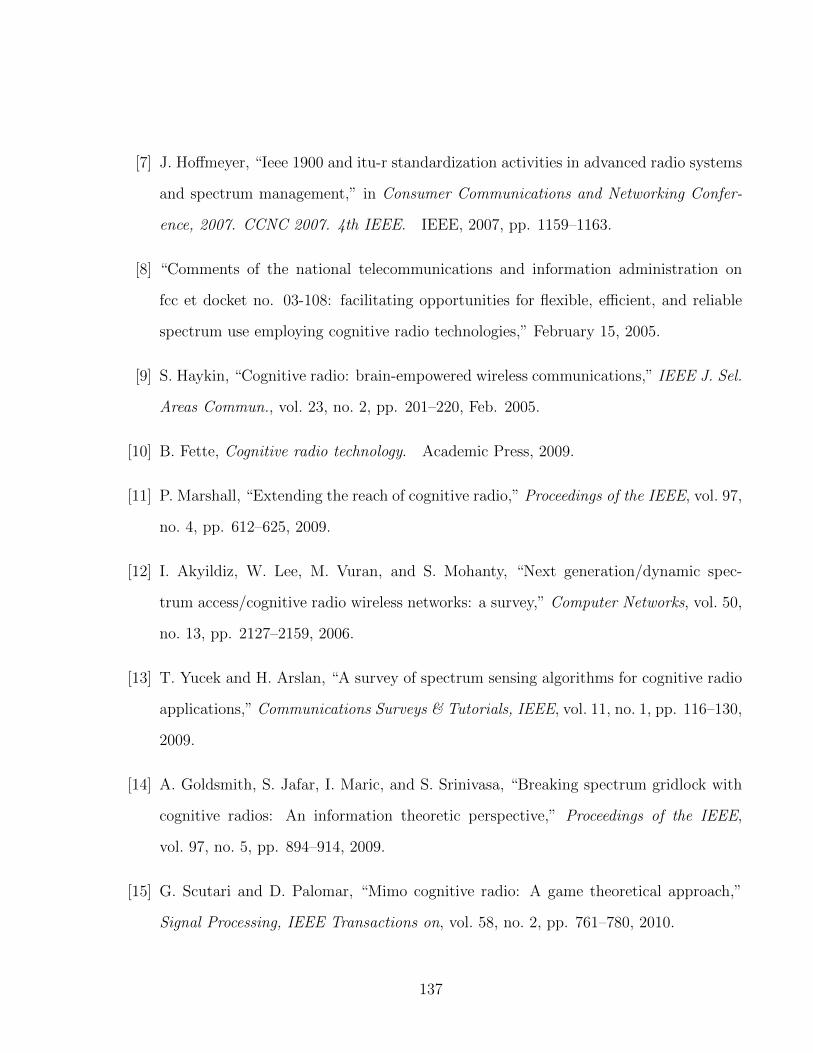
[7] J. Hoffmeyer, “Ieee 1900 and itu-r standardization activities in advanced radio systems
and spectrum management,” in Consumer Communications and Networking Confer-
ence, 2007. CCNC 2007. 4th IEEE. IEEE, 2007, pp. 1159–1163.
[8] “Comments of the national telecommunications and information administration on
fcc et docket no. 03-108: facilitating opportunities for flexible, efficient, and reliable
spectrum use employing cognitive radio technologies,” February 15, 2005.
[9] S. Haykin, “Cognitive radio: brain-empowered wireless communications,” IEEE J. Sel.
Areas Commun., vol. 23, no. 2, pp. 201–220, Feb. 2005.
[10] B. Fette, Cognitive radio technology. Academic Press, 2009.
[11] P. Marshall, “Extending the reach of cognitive radio,” Proceedings of the IEEE, vol. 97,
no. 4, pp. 612–625, 2009.
[12] I. Akyildiz, W. Lee, M. Vuran, and S. Mohanty, “Next generation/dynamic spec-
trum access/cognitive radio wireless networks: a survey,” Computer Networks, vol. 50,
no. 13, pp. 2127–2159, 2006.
[13] T. Yucek and H. Arslan, “A survey of spectrum sensing algorithms for cognitive radio
applications,” Communications Surveys & Tutorials, IEEE, vol. 11, no. 1, pp. 116–130,
2009.
[14] A. Goldsmith, S. Jafar, I. Maric, and S. Srinivasa, “Breaking spectrum gridlock with
cognitive radios: An information theoretic perspective,” Proceedings of the IEEE,
vol. 97, no. 5, pp. 894–914, 2009.
[15] G. Scutari and D. Palomar, “Mimo cognitive radio: A game theoretical approach,”
Signal Processing, IEEE Transactions on, vol. 58, no. 2, pp. 761–780, 2010.
137

[16] C. Clancy, J. Hecker, E. Stuntebeck, and T. O’Shea, “Applications of machine learning
to cognitive radio networks,” Wireless Communications, IEEE, vol. 14, no. 4, pp. 47–
52, 2007.
[17] Q. Zhao and B. Sadler, “A Survey of Dynamic Spectrum Access,” IEEE Signal Process
Mag., vol. 24, no. 3, pp. 79–89, 2007.
[18] G. Bianchi, “Performance analysis of the IEEE 802. 11 distributed coordination func-
tion,” IEEE Journal on selected areas in communications, vol. 18, no. 3, pp. 535–547,
2000.
[19] H. Wang and N. Moayeri, “Finite-state markov channel-a useful model for radio com-
munication channels,” Vehicular Technology, IEEE Transactions on, vol. 44, no. 1, pp.
163–171, 1995.
[20] I. Nikiforov, “A generalized change detection problem,” IEEE Trans. Inf. Theory,
vol. 41, no. 1, pp. 171–187, 1995.
[21] J. Chamberland and V. Veeravalli, “Wireless sensors in distributed detection applica-
tions,” IEEE Signal Processing Magazine, vol. 24, no. 3, p. 16, 2007.
[22] A. Tartakovsky, B. Rozovskii, R. Blazek, and H. Kim, “A Novel Approach to Detection
of Intrusions in Computer Networks via Adaptive Sequential and Batch-Sequential
Change-Point Detection Methods,” IEEE Trans. Signal Process., vol. 54, no. 9, p.
3372, 2006.
[23] A. Adya, P. Bahl, R. Chandra, and L. Qiu, “Architecture and techniques for diagnos-
ing faults in IEEE 802.11 infrastructure networks,” in Proceedings of the 10th annual
international conference on Mobile computing and networking. ACM New York, NY,
USA, 2004, pp. 30–44.
138

[24] S. Rayanchu, A. Mishra, D. Agrawal, S. Saha, and S. Banerjee, “Diagnosing wireless
packet losses in 802.11: Separating collision from weak signal,” in IEEE INFOCOM
2008. The 27th Conference on Computer Communications, 2008, pp. 735–743.
[25] D. Giustiniano, D. Malone, D. Leith, and K. Papagiannaki, “Experimental assessment
of 802.11 MAC layer channel estimators,” IEEE Commun. Lett., vol. 11, no. 12, pp.
961–963, 2007.
[26] FCC, “Docket No 03-322 Notice of Proposed Rule Making and Order,” 2003.
[27] E. Adamopoulou, K. Demestichas, and M. Theologou, “Enhanced estimation of con-
figuration capabilities in cognitive radio,” IEEE Commun. Mag., vol. 46, no. 4, pp.
56–63, 2008.
[28] I. Akyildiz, W. Lee, M. Vuran, and S. Mohanty, “NeXt generation/dynamic spec-
trum access/cognitive radio wireless networks: A survey,” Computer Networks, vol. 50,
no. 13, pp. 2127–2159, 2006.
[29] L. Giupponi and A. Perez-Neira, “Fuzzy-based Spectrum Handoff in Cognitive Ra-
dio Networks,” in 3rd International Conference on Cognitive Radio Oriented Wireless
Networks and Communications. CrownCom 2008., 2008, pp. 1–6.
[30] Y. Xing, C. Mathur, M. Haleem, R. Chandramouli, and K. Subbalakshmi, “Dynamic
Spectrum Access with QoS and Interference Temperature Constraints,” IEEE Trans.
Mob. Comput., pp. 423–433, 2007.
[31] H. Rahul, N. Kushman, D. Katabi, C. Sodini, and F. Edalat, “Learning to share:
narrowband-friendly wideband networks,” ACM SIGCOMM Computer Communica-
tion Review, vol. 38, no. 4, pp. 147–158, 2008.
139

[32] N. Kundargi and A. Tewfik, “A novel parallelized goodness-of-Fit test based Dynamic
Spectrum access technique for Cognitive Radio Networks,” in Communications, Con-
trol and Signal Processing (ISCCSP), 2010 4th Int. Symposium on. IEEE, pp. 1–5.
[33] ——, “A nonparametric sequential kolmogorov-smirnov test for transmit opportunity
detection at the MAC layer,” in Signal Processing Advances in Wireless Communica-
tions, 2009. SPAWC’09. IEEE 10th Workshop on. IEEE, 2009, pp. 101–105.
[34] ——, “ProTOMAC: Proactive Transmit Opportunity Detection at the MAC Layer
for Cognitive Radios,” in IEEE International Conference on Communications (ICC),
2010.
[35] S. Kim, E. Dall’Anese, and G. Giannakis, “Cooperative spectrum sensing for cogni-
tive radios using kriged kalman filtering,” Selected Topics in Signal Processing, IEEE
Journal of, no. 99, pp. 1–1, 2011.
[36] M. Papadopouli, H. Shen, E. Raftopoulos, M. Ploumidis, and F. Hernandez-Campus,
“Short-term traffic forecasting in a campus-wide wireless network,” in Personal, Indoor
and Mobile Radio Communications, 2005. PIMRC 2005. IEEE 16th International
Symposium on, vol. 3. IEEE, 2005, pp. 1446–1452.
[37] C. Sarr, C. Chaudet, G. Chelius, and I. Lassous, “Bandwidth Estimation for IEEE
802.11-Based Ad Hoc Networks,” IEEE Trans. Mob. Comput., vol. 7, no. 10, pp.
1228–1241, 2008.
[38] A. Toledo and X. Wang, “Robust Detection of MAC Layer Denial-of-Service Attacks
in CSMA/CA Wireless Networks,” IEEE Trans. Inf. Forensics Secur., vol. 3, no. 3,
pp. 347–358, 2008.
140

[39] N. Kundargi and A. Tewfik, “Sensing of Transmission Opportunities at the Medium
Access Control Layer for Cognitive Radio Networks,” in 3rd International Conference
on Wireless VITAE, 2009.
[40] R. D’Agostino and M. Stephens, “Goodness-of-fit techniques,” Marcel Dekker, Inc.
New York, NY, USA, p. 560, 1986.
[41] M. Stephens, “EDF statistics for goodness of fit and some comparisons,” Journal of
the American Statistical Association, vol. 69, no. 347, pp. 730–737, 1974.
[42] W. Conover, Practical Nonparametric Statistics. Wiley, 1999.
[43] D. Quade, “On the Asymptotic Power of the One-Sample Kolmogorov-Smirnov Tests,”
Ann. Math. Statist, vol. 36, no. 3, pp. 1000–1018, 1964.
[44] A. Kolmogoroff, “Sulla determinazione empirica di una legge di distribuzione,” Giorn.
1st. Ital. Attuari, vol. 4, pp. 83–91, 1933.
[45] J. Durbin, Distribution Theory for Tests Based on the Sample Distribution Function.
Society for Industrial Mathematics, 1973.
[46] F. Massey, “The Kolmogorov-Smirnov test for goodness of fit,” Journal of the Ameri-
can Statistical Association, vol. 46, no. 253, pp. 68–78, 1951.
[47] A. Stuart, J. Ord, and S. Arnold, “Kendalls Advanced Theory of Statistics, vol. 2A,”
London: Edward Arnold, 1999.
[48] D. Hawkins, “Retrospective and sequential tests for a change in distribution based
on kolmogorov-smirnov-type statistics,” Sequential Analysis, vol. 7, no. 1, pp. 23–51,
1988.
[49] D. Darling, “The Kolmogorov-Smirnov, Cramer-von Mises Tests,” Ann. Math. Statist,
vol. 28, no. 4, pp. 823–838, 1957.
141

[50] T. Anderson and D. Darling, “A test of goodness of fit,” Journal of the American
Statistical Association, pp. 765–769, 1954.
[51] J. Rodriguez and A. Viollaz, “A Cramer: von Mises type goodness of fit test with as-
symetric weight function,” Communications in statistics. Theory and methods, vol. 24,
no. 4, pp. 1095–1120, 1995.
[52] M. Basseville, “Distance measures for signal processing and pattern recognition,” Sig-
nal Processing, vol. 18, no. 4, pp. 349–369, 1989.
[53] S. Ali and S. Silvey, “A general class of coefficients of divergence of one distribution
from another,” J. Roy. Statist. Soc. Ser. B, vol. 28, no. 131-142, p. 213, 1966.
[54] S. Kullback and R. Leibler, “On information and sufficiency,” Annals of Mathematical
Statistics, vol. 22, no. 1, pp. 79–86, 1951.
[55] H. Jeffreys, “An Invariant Form for the Prior Probability in Estimation Problems,”
Proceedings of the Royal Society of London. Series A, Mathematical and Physical
Sciences (1934-1990), vol. 186, no. 1007, pp. 453–461, 1946.
[56] H. Chernoff, “A measure of asymptotic efficiency for tests of a hypothesis based on the
sum of observations,” Annals of Mathematical Statistics, vol. 23, no. 4, pp. 493–507,
1952.
[57] P. Halmos, Measure Theory. Springer-Verlag Berlin and Heidelberg GmbH & Co. K,
1974.
[58] A. Bhattacharyya, “On a measure of divergence between two statistical populations
defined by their probability distributions,” Bull. Calcutta Math. Soc, vol. 35, no.
99-109, p. 4, 1943.
142
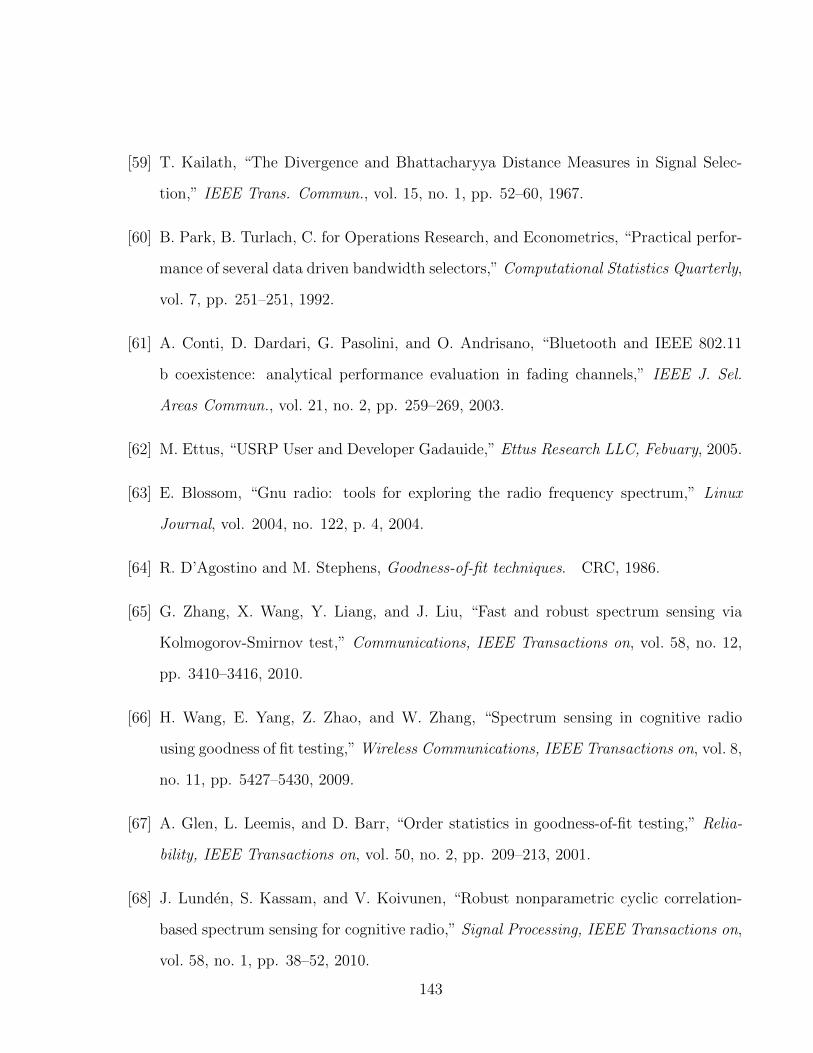
[59] T. Kailath, “The Divergence and Bhattacharyya Distance Measures in Signal Selec-
tion,” IEEE Trans. Commun., vol. 15, no. 1, pp. 52–60, 1967.
[60] B. Park, B. Turlach, C. for Operations Research, and Econometrics, “Practical perfor-
mance of several data driven bandwidth selectors,” Computational Statistics Quarterly,
vol. 7, pp. 251–251, 1992.
[61] A. Conti, D. Dardari, G. Pasolini, and O. Andrisano, “Bluetooth and IEEE 802.11
b coexistence: analytical performance evaluation in fading channels,” IEEE J. Sel.
Areas Commun., vol. 21, no. 2, pp. 259–269, 2003.
[62] M. Ettus, “USRP User and Developer Gadauide,” Ettus Research LLC, Febuary, 2005.
[63] E. Blossom, “Gnu radio: tools for exploring the radio frequency spectrum,” Linux
Journal, vol. 2004, no. 122, p. 4, 2004.
[64] R. D’Agostino and M. Stephens, Goodness-of-fit techniques. CRC, 1986.
[65] G. Zhang, X. Wang, Y. Liang, and J. Liu, “Fast and robust spectrum sensing via
Kolmogorov-Smirnov test,” Communications, IEEE Transactions on, vol. 58, no. 12,
pp. 3410–3416, 2010.
[66] H. Wang, E. Yang, Z. Zhao, and W. Zhang, “Spectrum sensing in cognitive radio
using goodness of fit testing,” Wireless Communications, IEEE Transactions on, vol. 8,
no. 11, pp. 5427–5430, 2009.
[67] A. Glen, L. Leemis, and D. Barr, “Order statistics in goodness-of-fit testing,” Relia-
bility, IEEE Transactions on, vol. 50, no. 2, pp. 209–213, 2001.
[68] J. Lunden, S. Kassam, and V. Koivunen, “Robust nonparametric cyclic correlation-
based spectrum sensing for cognitive radio,” Signal Processing, IEEE Transactions on,
vol. 58, no. 1, pp. 38–52, 2010.
143

[69] Y. Zeng and Y. Liang, “Eigenvalue-based spectrum sensing algorithms for cognitive
radio,” Communications, IEEE Transactions on, vol. 57, no. 6, pp. 1784–1793, 2009.
[70] S. Kassam, “A bibliography on nonparametric detection,” IEEE Transactions on In-
formation Theory, vol. 26, pp. 595–602, 1980.
[71] B. Seyfe and A. Sharafat, “Signed-rank nonparametric multiuser detection in non-
Gaussian channels,” Information Theory, IEEE Transactions on, vol. 51, no. 4, pp.
1478–1486, 2005.
[72] H. Chen, P. Varshney, S. Kay, and J. Michels, “Noise enhanced nonparametric de-
tection,” Information Theory, IEEE Transactions on, vol. 55, no. 2, pp. 499–506,
2009.
[73] Y. Zeng, Y. Liang, A. Hoang, and R. Zhang, “A review on spectrum sensing for
cognitive radio: challenges and solutions,” EURASIP Journal on Advances in Signal
Processing, vol. 2010, pp. 2–2, 2010.
[74] M. Schervish, “P Values: What They Are and What They Are Not.” The American
Statistician, vol. 50, no. 3, 1996.
[75] J. Hoenig and D. Heisey, “The abuse of power,” The American Statistician, vol. 55,
no. 1, pp. 19–24, 2001.
[76] D. Donoho and J. Jin, “Higher criticism for detecting sparse heterogeneous mixtures,”
The Annals of Statistics, vol. 32, no. 3, pp. 962–994, 2004.
[77] J. Angus, “The probability integral transform and related results,” SIAM review,
vol. 36, no. 4, pp. 652–654, 1994.
[78] L. Jager and J. Wellner, “Goodness-of-fit tests via phi-divergences,” The Annals of
Statistics, vol. 35, no. 5, pp. 2018–2053, 2007.
144

[79] N. Cressie, “Multinomial goodness-of-fit tests,” Journal of the Royal Statistical Society.
Series B (Methodological), vol. 46, no. 3, pp. 440–464, 1984.
[80] F. Liese and I. Vajda, “On divergences and informations in statistics and information
theory,” Information Theory, IEEE Transactions on, vol. 52, no. 10, pp. 4394–4412,
2006.
[81] I. Vajda, Theory of statistical inference and information. Kluwer Academic Publishers
Boston, 1989.
[82] R. Berk and D. Jones, “Goodness-of-fit test statistics that dominate the kolmogorov
statistics,” Probability Theory and Related Fields, vol. 47, no. 1, pp. 47–59, 1979.
[83] J. Wellner and V. Koltchinskii, “A note on the asymptotic distribution of berk-jones
type statistics under the null hypothesis,” High Dimensional Probability III, pp. 321–
332, 2003.
[84] L. Jager and J. Wellner, “A new goodness of fit test: the reversed berk-jones statistic,”
2004.
[85] J. Einmahl and I. McKeague, “Empirical likelihood based hypothesis testing,” Bernoulli,
vol. 9, no. 2, pp. 267–290, 2003.
[86] D. Middleton, “Non-Gaussian noise models in signal processing for telecommunica-
tions: New methods an results for class A and class B noise models,” Information
Theory, IEEE Transactions on, vol. 45, no. 4, pp. 1129–1149, 1999.
[87] A. Chopra, K. Gulati, B. Evans, K. Tinsley, and C. Sreerama, “Performance bounds of
MIMO receivers in the presence of radio frequency interference,” in IEEE International
Conference on Acoustics, Speech and Signal Processing, 2009, pp. 2817–2820.
145

[88] L. Liu and M. Amin, “Performance analysis of GPS receivers in non-Gaussian noise
incorporating precorrelation filter and sampling rate,” Signal Processing, IEEE Trans-
actions on, vol. 56, no. 3, pp. 990–1004, 2008.
[89] R. Donahue, “A Note on Information Seldom Reported Via the P Value.” The Amer-
ican Statistician, vol. 53, no. 4, 1999.
[90] E. Lehmann and J. Romano, Testing statistical hypotheses. Springer Verlag, 2005.
[91] S. Metchev and G. JE, “A two-dimensional Kolmogorov–Smirnov test for crowded
field source detection: ROSAT sources in NGC 6397,” Monthly Notices of the Royal
Astronomical Society, vol. 335, no. 1, pp. 73–83, 2002.
[92] R. Lopes, I. Reid, and P. Hobson, “The two-dimensional Kolmogorov-Smirnov test,”
in XI International Workshop on Advanced Computing and Analysis Techniques in
Physics Research, Nikhef, Amsterdam, the Netherlands, April 23-27, 2007, 2007.
[93] G. Fasano and A. Franceschini, “A multidimensional version of the Kolmogorov-
Smirnov test,” Monthly Notices of the Royal Astronomical Society, vol. 225, pp. 155–
170, 1987.
[94] M. Noe, “The calculation of distributions of two-sided Kolmogorov-Smirnov type
statistics,” The Annals of Mathematical Statistics, vol. 43, no. 1, pp. 58–64, 1972.
[95] K. Kim, I. Akbar, K. Bae, J. Urn, C. Spooner, and J. Reed, “Cyclostationary ap-
proaches to signal detection and classification in cognitive radio,” in 2nd IEEE Inter-
national Symposium on New Frontiers in Dynamic Spectrum Access Networks, 2007.
DySPAN 2007, 2007, pp. 212–215.
[96] Z. Quan, S. Cui, A. Sayed, and H. Poor, “Optimal Multiband Joint Detection for
Spectrum Sensing in Cognitive Radio Networks,” IEEE Trans. Signal Process., vol. 57,
no. 3, pp. 1128–1140, 2009.
146

[97] C. Cordeiro, K. Challapali, and D. Birru, “IEEE 802.22: An Introduction To The First
Wireless Standard Based On Cognitive Radios,” Journal of Communications, vol. 1,
no. 1, pp. 38–47, 2006.
[98] A. Sahai, N. Hoven, and R. Tandra, “Some Fundamental Limits on Cognitive Radio,”
in Allerton Conference on Communication, Control, and Computing, 2004.
[99] D. Cabric, A. Tkachenko, and R. Brodersen, “Experimental Study of Spectrum Sensing
Based on Energy Detection and Network Cooperation,” in 1st International Workshop
on Technology and Policy for Accessing Spectrum, TAPAS., 2006.
[100] H. Urkowitz, “Energy detection of unknown deterministic signals,” Proceedings of the
IEEE, vol. 55, no. 4, pp. 523–531, 1967.
[101] D. Cabric, S. Mishra, and R. Brodersen, “Implementation issues in spectrum sensing
for cognitive radios,” in Signals, Systems and Computers, 2004. Conference Record of
the Thirty-Eighth Asilomar Conference on, vol. 1. Ieee, 2004, pp. 772–776.
[102] S. Chang, “Analysis of proposed sensing schemes: Ieee 802.22-06/0032r0,” 2006.
[103] A. Ghasemi and E. Sousa, “Collaborative spectrum sensing for opportunistic access
in fading environments,” in First IEEE International Symposium on New Frontiers in
Dynamic Spectrum Access Networks, 2005. DySPAN., 2005, pp. 131–136.
[104] R. Blum, S. Kassam, and H. Poor, “Distributed detection with multiple sensors I.
Advanced topics,” Proceedings of the IEEE, vol. 85, no. 1, pp. 64–79, 1997.
[105] N. Kundargi and A. Tewfik, “Hierarchical Sequential Detection In The Context Of Dy-
namic Spectrum Access For Cognitive Radios,” in 14th IEEE International Conference
on Electronics, Circuits and Systems. ICECS, 2007.
147

[106] ——, “Sequential pilot sensing of ATSC signals in IEEE 802.22 cognitive radio net-
works,” IEEE International Conference on Acoustics, Speech and Signal Processing.
ICASSP, 2008.
[107] T. Lai, “Sequential analysis: some classical problems and new challenges,” Statistica
Sinica, vol. 11, no. 2, pp. 303–350, 2001.
[108] L. Lai, Y. Fan, and H. Poor, “Quickest Detection in Cognitive Radio: A Sequen-
tial Change Detection Framework,” in IEEE Global Telecommunications Conference.
GLOBECOM, 2008.
[109] Y. Xin, H. Zhang, Z. Ho, V. Lau, R. Cheng, V. Mordachev, and S. Loyka, “A
Simple Sequential Spectrum Sensing Scheme for Cognitive Radio,” Arxiv preprint
arXiv:0905.4684, 2009.
[110] S. Kay, Fundamentals of Statistical Signal Processing. Prentice Hall PTR, 1993.
[111] R. Chen, J. Park, and K. Bian, “Robust Distributed Spectrum Sensing in Cognitive
Radio Networks,” in 27th IEEE Conference on Computer Communications, INFO-
COM 2008.
[112] A. Wald, Sequential analysis. Dover Publications, 2004.
[113] M. Simon, Probability Distributions Involving Gaussian Random Variables: A Hand-
book for Engineers and Scientists. Kluwer Academic Publishers, 2002.
[114] J. Coon, M. Sandell, M. Beach, J. McGeehan, and T. Bristol, “Channel and Noise
Variance Estimation and Tracking Algorithms for Unique-word Based Single-carrier
Systems,” IEEE Transactions on Wireless Communications, vol. 5, no. 6, pp. 1488–
1496, 2006.
148

[115] Z. Botev, “Nonparametric Density Estimation via Diffusion Mixing,” The University
of Queensland, Postgraduate Series, Nov, 2007.
[116] P. Hall, S. Sheather, M. Jones, and J. Marron, “On Optimal Data-based Bandwidth
Selection in Kernel Density Estimation,” Biometrika, vol. 78, no. 2, pp. 263–269, 1991.
[117] C. Stevenson, G. Chouinard, Z. Lei, W. Hu, S. Shellhammer, and W. Caldwell, “Ieee
802.22: The first cognitive radio wireless regional area network standard,” Communi-
cations Magazine, IEEE, vol. 47, no. 1, pp. 130–138, 2009.
[118] M. Ghosh, “Text on fft-based pilot sensing-for informative annex on sensing tech-
niques,” in IEEE 802.22 Meeting Doc, 2007.
[119] C. Cordeiro, M. Ghosh, D. Cavalcanti, and K. Challapali, “Spectrum sensing for
dynamic spectrum access of tv bands,” in Cognitive Radio Oriented Wireless Net-
works and Communications, 2007. CrownCom 2007. 2nd International Conference
on. IEEE, 2007, pp. 225–233.
[120] S. Mathur, R. Tandra, S. Shellhammer, and M. Ghosh, “Initial signal processing of
captured dtv signals for evaluation of detection algorithms,” IEEE 802.22-06/0158r4,
2006.
149
Recommended