Nonparametric Change-Point Tests for Long-Range
Dependent Data
Herold Dehling
Fakultat fur Mathematik, Ruhr-Universitat Bochum
Aeneas Rooch
Fakultat fur Mathematik, Ruhr-Universitat Bochum
Murad S. Taqqu
Department of Mathematics and Statistics, Boston University
March 2, 2012
Abstract
We propose a nonparametric change-point test for long-range dependent data,
which is based on the Wilcoxon two-sample test. We derive the asymptotic distri-
bution of the test statistic under the null-hypothesis that no change occured. In a
simulation study, we compare the power of our test with the power of a test which is
based on differences of means. The results of the simulation study show that in the case
of Gaussian data, our test has only slightly smaller power than the difference-of-means
test. For heavy-tailed data, our test outperforms the difference-of-means test.
Running Head: Change-Point Tests for LRD Data
Keywords: Change-point problem, functional limit theorem, long memory, long-range
dependent data, nonparametric test, Wilcoxon two-sample rank test.
1
1 Introduction and Statement of Main Results
In this paper we study change-point problems in long-range dependent time series. Specif-
ically we consider the model where the observations are generated by a stochastic process
(Xi)i≥1 of the type
Xi = µi + εi,
where (εi)i≥1 is a long-range dependent stationary process with mean zero, and where (µi)i≥1
are the unknown means. We focus on the case when (εi)i≥1 is an instantaneous functional
of a stationary Gaussian process with non-summable covariances, i.e.
εi = G(ξi), i ≥ 1.
We assume that (ξi)i≥1 is a mean-zero Gaussian process with E(ξ2i ) = 1 and long-range
dependence, that is, with autocovariance function
ρ(k) = k−DL(k), k ≥ 1, (1)
where 0 < D < 1, and where L(k) is a slowly varying function. Moreover, G : R → R is a
measurable function satisfying E(G(ξi)) = 0.
Based on observations X1, . . . , Xn, we wish to test the hypothesis
H : µ1 = . . . = µn
that there is no change in the means of the data against the alternative
A : µ1 = . . . = µk 6= µk+1 = . . . = µn for some k ∈ {1, . . . , n− 1}.
We shall refer to this test problem as (H,A).
In the case of independent observations, change-point problems have been much inves-
tigated, and both parametric as well as nonparametric tests have been studied. For an
excellent survey, see the monograph by Csorgo and Horvath (1997). There are also many
results for weakly dependent observations. E.g., Ling (2007) studies the asymptotic distri-
bution of the Wald test for parameter changes in near epoch dependent processes. Aue,
Hormann, Horvath and Reimherr (2009) study tests for detecting breaks in the covariance
structure of multivariate time series. Wied, Kramer and Dehling (2011) study change-points
in the correlation structure of near epoch dependent processes.
In the case of long-range dependent data, much less is known. Csorgo and Horvath (1997)
study so-called cusum tests (cumulative sum tests) for changes in the mean, which are based
2
on statistics of the type
max1≤k≤n
∣∣∣∣∣1kk∑i=1
Xi −1
n
n∑i=1
Xi
∣∣∣∣∣ .Kramer, Sibbertsen and Kleiber (2002) observe that the presence of long-range dependence
might lead to false rejection of the hypothesis of stationarity in change-point tests. Berkes,
Horvath, Kokoszka and Shao (2006) propose cusum type tests for discriminating between
long-range dependence and changes in the mean of a weakly dependent process. Giraitis,
Leipus and Surgailis (1996) consider change-point problems for linear processes where they
test the hypothesis of stationarity against the alternative of some break. Their tests are
based on supremum functionals of the empirical process. Horvath and Kokoszka (1997) study
cusum tests for change points for Gaussian processes. Wang (2003) studies cusum tests for
change-points in multivariate processes that are subordinated to a Gaussian process. Wang
(2008b) studies cusum tests for linear processes.
In the present paper we want to investigate rank tests for changes in the mean. An-
toch, Huskova, Janic and Ledwina (2008) studied rank tests for i.i.d. observations. Wang
(2008a) investigated rank tests for change-points in long-range dependent linear processes.
In this paper, we study rank tests for changes in the mean of long-range dependent processes
that have a representation as instantaneous nonlinear functionals of stationary Gaussian
processes.
Tests for change-point problems usually start from the two-sample problem that one
obtains when the change-point is regarded as being known, that is, where for a given k ∈{1, . . . , n− 1}, the alternative is
Ak : µ1 = . . . = µk 6= µk+1 = . . . = µn.
For the test problem (H,Ak), the Wilcoxon two-sample rank test is a commonly used non-
parametric test. The Wilcoxon test rejects for large and small values of the test statistic
Wk,n =k∑i=1
n∑j=k+1
1{Xi≤Xj}.
Wk,n counts the number of times the second part of the sample exceeds the first part of the
sample. Note that this is the Mann-Whitney U -statistic representation of Wilcoxon’s rank
test statistic; see e.g. Lehmann (1975).
Tests for the change-point problem (H,A), where one does not suppose that k is known,
can be based on the vector of test statistics W1,n, . . . ,Wn−1,n. In a parametric model, the
generalized likelihood ratio test rejects for large values of the maximum of the test statistics
3
obtained for the two-sample problems (H,Ak); see e.g. Csorgo and Horvath (1997). Also
in the nonparametric case, a common procedure is to reject the null hypothesis for large
values of Wn = maxk=1,...,n−1 |Wk,n|, though one could in principle take other functions of
W1,n, . . . ,Wn−1,n.
In order to set the critical values of the test, we need to know the distribution of Wn
under the null hypothesis of no change. Since the exact distribution is hard to obtain, we
consider the asymptotic distribution for a large sample size. To this end we consider the
process
Wn,[nλ] =
[nλ]∑i=1
n∑j=[nλ]+1
1{Xi≤Xj}, 0 ≤ λ ≤ 1,
parametrized by λ. After centering and normalizing, we obtain the process
Wn(λ) =1
n dn
[nλ]∑i=1
n∑j=[nλ]+1
(1{Xi≤Xj} −
∫RF (x)dF (x)
), 0 ≤ λ ≤ 1. (2)
Observe that the centering constant∫R F (x)dF (x) equals E(1{X1≤X′
1}), where X ′1 is an
independent copy of X1. The latter is the proper normalization as the dependence between
Xi and Xj vanishes asymptotically when |j − i| → ∞. If the distribution function F is
continuous, we get∫R F (x)dF (x) = 1
2. Note that under the null hypothesis, the distribution
of Wn(λ) does not depend on the common mean µ := µ1 = . . . = µn. Thus, we may assume
without loss of generality that µ = 0 and hence that Xi = G(ξi).
In order to analyze the asymptotic distribution of the process (Wn(λ))0≤λ≤1, we apply
the empirical process invariance principle of Dehling and Taqqu (1989) to the sequence
(G(ξi))i≥1. We consider the Hermite expansion
1{G(ξi)≤x} − F (x) =∞∑q=1
Jq(x)
q!Hq(ξi),
where Hq is the q-th order Hermite polynomial and where
Jq(x) = EHq(ξi)1{G(ξi)≤x}.
We define the Hermite rank of the class of functions {1{G(ξi)≤x} − F (x), x ∈ R}, by
m := min{q ≥ 1 : Jq(x) 6= 0 for some x ∈ R}, (3)
and the normalizing constants
d2n = Var
(n∑j=1
Hm(ξj)
). (4)
4
We make the further assumption that 0 < D < 1m
, in which case
d2n ∼ cm n2−mDLm(n), (5)
where cm = 2m!(1−Dm)(2−Dm)
. Here we use the symbol an ∼ bn to denote that an/bn → 1 as
n → ∞. Then by the two-parameter empirical process invariance principle of Dehling and
Taqqu (1989),(d−1n [nλ](F[nλ](x)− F (x))
)x∈[−∞,∞],λ∈[0,1] →
(Jm(x)
m!Zm(λ)
)x∈[−∞,∞],λ∈[0,1]
,
weakly in D([−∞,∞]×[0, 1]), where (Zm(λ))λ∈[0,1] is an m-th order Hermite process, defined
in Taqqu (1979), formula (1.3). A spectral representation of Zm is given in formula (1.7)
of Dehling and Taqqu (1989). Observe the separation of variables in the limit: the limiting
process Zm(x, λ) is expressible as Jm(x)m!
Zm(λ).
The process (Zm(λ))λ≥0 is self-similar with parameter
H = 1− mD
2∈ (
1
2, 1),
that is, Zm(c λ) and cHZm(λ) have the same finite-dimensional distributions for all constants
c > 0.1 The process Zm(λ) is not Gaussian when m ≥ 2. When m = 1, Z1(λ) is the standard
Gaussian fractional Brownian motion, often denoted BH(λ). It is Gaussian with mean zero
and covariance
E (Z1(λ1)Z1(λ2)) =1
2
{λ2H1 + λ2H2 − |λ1 − λ2|2H
}(6)
Theorem 1 Suppose that (ξi)i≥1 is a stationary Gaussian process with mean zero, variance
1, and autocovariance function as in (1) with 0 < D < 1m
. Moreover let G : R → R be a
measurable function and define
Xk = G(ξk).
Assume that Xk has a continuous distribution function F . Let m denote the Hermite rank
of the class of functions 1{G(ξi)≤x} − F (x), x ∈ R, as defined in (3) and let dn > 0 satisfy
(5). Then
1
n dn
[nλ]∑i=1
n∑j=[nλ]+1
(1{Xi≤Xj} −
∫RF (x)dF (x)
), 0 ≤ λ ≤ 1, (7)
converges in distribution towards the process
1
m!(Zm(λ)− λZm(1))
∫RJm(x)dF (x), 0 ≤ λ ≤ 1.
1Do not confuse the index H, which is called Hurst parameter with the other H’s used in this paper to
denote hypothesis and Hermite polynomial.
5
2 Proof of Theorem 1
We introduce the empirical distribution functions of the first k and the last (n− k) observa-
tions, respectively:
Fk(x) =1
k
k∑i=1
1{Xi≤x}
Fk+1,n(x) =1
n− k
n∑i=k+1
1{Xi≤x}
so that [nλ]F[nλ](x) =∑[nλ]
i=1 1{Xi≤x} and (n − [nλ])F[nλ]+1,n =∑n
i=[nλ]+1 1{Xi≤x}. Then we
obtain the following representation
[nλ]∑i=1
n∑j=[nλ]+1
(1{Xi≤Xj} −
∫RF (x)dF (x)
)(8)
= [nλ]n∑
j=[nλ]+1
(F[nλ](Xj)−
∫RF (x)dF (x)
)
= [nλ](n− [nλ])
(∫RF[nλ](x)dF[nλ]+1,n(x)−
∫RF (x)dF (x)
)= [nλ](n− [nλ])
∫R(F[nλ](x)− F (x))dF[nλ]+1,n(x)
+[nλ](n− [nλ])
∫RF (x)d(F[nλ]+1,n − F )(x)
= [nλ](n− [nλ])
∫R(F[nλ](x)− F (x))dF[nλ]+1,n(x)
−[nλ](n− [nλ])
∫R(F[nλ]+1,n(x)− F (x))dF (x),
where in the third line we used the relation E(K(X)) =∫RK(x)dF (x), where F and E are
respectively, the empirical distribution and the empirical mean of X, and where, in the final
step, we have used integration by parts, namely∫RGdF = 1 −
∫R F dG, if F and G are
two distribution functions. We now apply the empirical process non-central limit theorem
of Dehling and Taqqu (1989), which states that in the space D([−∞,∞]× [0, 1]), equipped
with the supremum norm,(d−1n [nλ](Fnλ(x)− F (x))
)x∈[−∞,∞],λ∈[0,1]
D−→(J(x)Z(λ))x∈[−∞,∞],λ∈[0,1], (9)
where
J(x) = Jm(x) and Z(λ) = Zm(λ)/m!.
6
Here,D−→ denotes convergence in distribution of random variables with values in the non-
separable metric space D = D([−∞,∞] × [0, 1]), as defined e.g. in Shorack and Wellner
(1986), Section 2.3. Given D-valued random variables (Wn)n≥1 and W , we say that Wn
converges in distribution to W if
Ef(Wn)→ Ef(W )
holds for all functions f : D → R that are bounded, uniformly continuous with respect to the
supremum norm on D and measurable with respect to the σ-field DB on D that is generated
by the open balls. We can then apply the Skorohod-Dudley-Wichura representation theorem;
see Theorem 2.3.4 in Shorack and Wellner (1986). Note that C([−∞,∞]×[0, 1]) is a separable
subset of D, and that P ((J(x)Z(λ))x∈[−∞,∞],λ∈[0,1] ∈ C([−∞,∞] × [0, 1])) = 1, since F is
assumed to be continuous. Thus the conditions of the Skorohod-Dudley-Wichura theorem
are met with Ms = C([−∞,∞] × [0, 1]). Hence we may assume without loss of generality
that convergence holds almost surely with respect to the supremum norm on the function
space D([0, 1]× [−∞,∞]), i.e.
supλ,x
∣∣d−1n [nλ](Fnλ(x)− F (x))− J(x)Z(λ)∣∣ −→ 0 a.s. (10)
Note that, by definition,
(n− [nλ])(F[nλ]+1,n(x)− F (x)) = n(Fn(x)− F (x))− [nλ](F[nλ](x)− F (x)). (11)
Applying (10) to each of the terms on the right-hand side of (11), we obtain the following
limit theorem for the two parameter empirical process of the observations X[nλ]+1, . . . , Xn.
supλ,x
∣∣d−1n (n− [nλ])(F[nλ]+1,n(x)− F (x))− J(x)(Z(1)− Z(λ))∣∣ −→ 0. (12)
Thus we get, for the first term in the right-hand side of (8),
1
n dn[nλ](n− [nλ])
∫R(F[nλ](x)− F (x))dF[nλ]+1,n(x)− (1− λ)
∫RJ(x)Z(λ)dF (x) (13)
=n− [nλ]
n
∫Rd−1n [nλ](F[nλ](x)− F (x))dF[nλ]+1,n(x)− n− [nλ]
n
∫RJ(x)Z(λ)dF (x)
+
{n− [nλ]
n− (1− λ)
}∫RJ(x)Z(λ)dF (x)
=n− [nλ]
n
∫R
{d−1n [nλ](F[nλ](x)− F (x))− J(x)Z(λ)
}dF[nλ]+1,n(x)
+n− [nλ]
n
∫RJ(x)Z(λ)d(F[nλ]+1,n − F )(x)
+
{n− [nλ]
n− (1− λ)
}∫RJ(x)Z(λ)dF (x).
7
The first term on the right-hand side converges to 0 almost surely, by (10). The third term
converges to zero as
sup0≤λ≤1
∣∣∣∣n− [nλ]
n− (1− λ)
∣∣∣∣→ 0.
Regarding the second term, note that∫R J(x)dF (x) = E(J(Xi)) and hence
n− [nλ]
n
∫RJ(x)Z(λ)d(F[nλ]+1,n − F )(x)
= Z(λ)1
n
n∑i=[nλ]+1
(J(Xi)− EJ(Xi))
= Z(λ)
1
n
n∑i=1
(J(Xi)− E(J(Xi)))−1
n
[nλ]∑i=1
(J(Xi)− E(J(Xi)))
.
By the ergodic theorem, 1n
∑ni=1(J(Xi)− E(J(Xi)))→ 0, almost surely. Thus, given ε > 0,
we can find n0 = n0(ε, ω) such that, for all n ≥ n0,
1
n
n∑i=1
(J(Xi)− E(J(Xi))) ≤ ε.
Hence, for n ≥ max{n0,1ε
max1≤k≤n0 |∑k
i=1(J(Xi)− E(J(Xi)))|}, we have
max1≤k≤n
∣∣∣∣∣k∑i=1
(J(Xi)− E(J(Xi)))
∣∣∣∣∣≤ max
(max
1≤k≤n0
∣∣∣∣∣k∑i=1
(J(Xi)− E(J(Xi)))
∣∣∣∣∣ , maxn0≤k≤n
∣∣∣∣∣k∑i=1
(J(Xi)− E(J(Xi)))
∣∣∣∣∣)
≤ ε n.
and thus
max1≤k≤n
∣∣∣∣∣k∑i=1
(J(Xi)− E(J(Xi)))
∣∣∣∣∣ = o(n), as n→∞, a.s. (14)
Hence (13) converges to zero almost surely, uniformly in λ ∈ [0, 1].
Regarding the second term on the right-hand side of (8) we obtain
1
n dn[nλ](n− [nλ])
∫R(F[nλ]+1,n − F (x))dF (x)− λ
∫RJ(x)(Z(1)− Z(λ))dF (x) (15)
=[nλ]
n
∫R
{d−1n (n− [nλ])(F[λn]+1,n(x)− F (x))− J(x)(Z(1)− Z(λ))
}dF (x)
−(λ− [nλ]
n
)∫RJ(x)(Z(1)− Z(λ))dF (x).
8
Both terms on the right-hand side converge to zero a.s., uniformly in λ ∈ [0, 1]. For the first
term, this follows from (12). For the second term, this holds since sup0≤λ≤1
∣∣∣ [nλ]n − λ∣∣∣ → 0,
as n → ∞. Using (8) and the fact that the right-hand sides of (13) and (15) converge to
zero uniformly in 0 ≤ λ ≤ 1, we have proved that the normalized Wilcoxon two-sample test
statistic (7) converges in distribution towards∫R(1− λ)Z(λ)J(x)dF (x)−
∫Rλ(Z(1)− Z(λ))J(x)dF (x), 0 ≤ λ ≤ 1.
Finally, we observe that∫R(1− λ)Z(λ)J(x)dF (x)−
∫Rλ(Z(1)− Z(λ))J(x)dF (x) = (Z(λ)− λZ(1))
∫RJ(x)dF (x),
and thus we have established Theorem 1. �
Remark 1 (1) In our proof we have used an integration by parts in order to express our test
statistic as a functional of the empirical process. A similar integration by parts technique
was used by Dehling and Taqqu (1989, 1991). Note that in the present paper, we use a one-
dimensional integration by parts formula, whereas Dehling and Taqqu use a two-dimensional
integration by parts. The latter would not work here, as the kernel 1{x≤y} does not have
locally bounded variation.
(2) As a corollary to Theorem 1, we obtain for fixed λ ∈ [0, 1] the asymptotic distribution of
the Wilcoxon two-sample test, where the two samples are
X1, . . . , X[nλ]
X[nλ]+1, . . . , Xn.
After centering and normalization, the corresponding test statistic is
Un =1
n dn
[nλ]∑i=1
n∑j=[nλ]+1
(1{Xi≤Xj} −
∫RF (x)dF (x)
).
From Theorem 1 we obtain that Un converges in distribution to
1
m!
(Zm(λ)− λZm(1)
)∫RJm(x)dF (x).
This can be rewritten as
1
m!
((1− λ)Zm(λ)− λ(Zm(1)− Zm(λ))
)∫RJm(x)dF (x),
an expression which is useful for the next remark.
9
(3) A different two-sample problem arises when we observe samples from two independent
long-range dependent processes (Xi)i≥1 and (X ′i)i≥1 with identical joint distributions. In this
case, the samples are
X1, . . . , X[nλ]
X ′1, . . . , X′n−[nλ].
The normalized two-sample Wilcoxon test statistic for this case is
U ′n =1
n dn
[nλ]∑i=1
n−[nλ]∑j=1
(1{Xi≤X′
j} −∫RF (x)dF (x)
).
Following the proof of Theorem 1, and making the appropriate changes where needed, one
can show that U ′n converges in distribution towards
1
m!((1− λ)Zm(λ)− λZ ′m(1− λ))
∫RJm(x)dF (x),
where (Z ′m(λ)) is an independent copy of (Zm(λ))0≤λ≤1. Note that the limit distributions in
the two models are different, as the joint distribution of (Zm(λ), Zm(1)−Zm(λ)) is different
from that of (Zm(λ), Z ′m(1− λ)). This is a result of the fact that the Hermite process does
not have independent increments.
Observe that this is in contrast to the short-range dependent case. In this situation, the
Wilcoxon two-sample test statistic has the same distribution in both models; see Dehling and
Fried (2012). Roughly speaking, the dependence washes away in the limit for short-range
dependence, but not for long-range dependence.
3 Application
In what follows, we will consider the model
Xi = µi +G(ξi), i = 1, . . . , n, (16)
where (ξi)i≥1 is a mean-zero Gaussian process with Var(ξi) = 1 and autocovariance function
ρ(k) satisfying (1). We wish to test the hypothesis
H : µ1 = . . . = µn (17)
against the alternative
A : µ1 = . . . = µk 6= µk+1 = . . . = µn for some k ∈ {1, . . . , n− 1}.
10
3.1 Wilcoxon-type rank test
The change-point test based on Wilcoxon’s rank test will reject the null hypothesis for large
values of
Wn =1
n dnmax
1≤k≤n−1
∣∣∣∣∣k∑i=1
n∑j=k+1
(1{Xi≤Xj} −
1
2
)∣∣∣∣∣ . (18)
We first note an invariance property of the test statistic Wn.
Lemma 1 The test statistic Wn is invariant under strictly monotone transformations of the
data, i.e.
1
n dnmax
1≤k≤n−1
∣∣∣∣∣k∑i=1
n∑j=k+1
(1{G(Xi)≤G(Xj)} −
1
2
)∣∣∣∣∣ =1
n dnmax
1≤k≤n−1
∣∣∣∣∣k∑i=1
n∑j=k+1
(1{Xi≤Xj} −
1
2
)∣∣∣∣∣for all strictly monotone functions G : R→ R.
Proof. If G is strictly increasing, this is obvious, as G(Xi) ≤ G(Xj) if and only if Xi ≤ Xj.
If G is strictly decreasing, G(Xi) ≤ G(Xj) if and only if Xj ≤ Xi, and thus
1{G(Xi)≤G(Xj)} = 1− 1{Xi≤Xj}.
Hence we get
k∑i=1
n∑j=k+1
(1{G(Xi)≤G(Xj)} −
1
2
)= −
k∑i=1
n∑j=k+1
(1{Xi≤Xj} −
1
2
),
and thus the lemma is proved. �
Since Xi = µi +G(ξi), under the null hypothesis,
Wn =1
n dnmax
1≤k≤n−1
∣∣∣∣∣k∑i=1
n∑j=k+1
(1{G(ξi)≤G(ξj)} −
1
2
)∣∣∣∣∣ . (19)
Thus, applying Theorem 1 and the continuous mapping theorem, under the null hypothesis,
Wn converges in distribution, as n→∞, to
sup0≤λ≤1
∣∣∣∣Zm(λ)
m!− λZm(1)
m!
∣∣∣∣ ∣∣∣∣∫RJm(x)dF (x)
∣∣∣∣ .In order to set critical values for the asymptotic test based on Wn, we need to calculate the
distribution of the last expression.
11
In what follows, we will assume that G is a strictly monotone function. In this case,
combining (19) and Lemma 1 we get that
Wn =1
n dnmax
1≤k≤n−1
∣∣∣∣∣k∑i=1
n∑j=k+1
(1{ξi≤ξj} −
1
2
)∣∣∣∣∣ .Note that in this case,
J1(x) = E(ξ1{ξ≤x}) =
∫ x
−∞tϕ(t)dt = −ϕ(x),
where ϕ(t) = 1√2πe−t
2/2 denotes the standard normal density function. In the last step, we
have used the fact that ϕ′(t) = −t ϕ(t). Thus J1(x) 6= 0 for all x and hence the class of
functions {1{ξ≤x}, x ∈ R} has Hermite rank m = 1. Moreover, as F is the normal distribution
function we obtain∫RJ1(x)dF (x) = −
∫R
ϕ(x)ϕ(x)dx =
∫R−(ϕ(s))2ds = − 1
2√π. (20)
We have thus proved the following theorem.
Theorem 2 Let (ξi)i≥1 be a stationary Gaussian process with mean zero, variance 1 and
autocovariance function as in (1) with 0 < D < 1. Moreover, let G : R → R be a strictly
monotone function and define Xi = µi + G(ξi). Then, under the null hypothesis H: µ1 =
. . . = µn, the test statistic Wn, as defined in (18), converges in distribution towards
1
2√π
sup0≤λ≤1
|Z1(λ)− λZ1(1)|,
where (Z1(λ))λ≥0 denotes the standard fractional Brownian motion process with Hurst pa-
rameter H = 1 − D/2 ∈ (1/2, 1). The normalizing constant in (18) satisfies n dn ∼(L(n)
(1−D)(1−D/2)
)1/2n2−D/2.
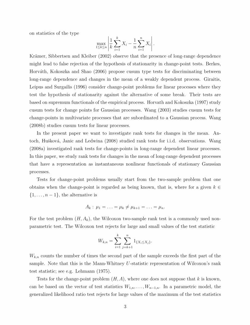
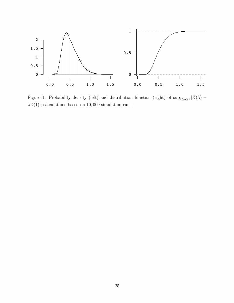
– Insert Figure 1 here –
We have evaluated the distribution of sup0≤λ≤1 |Z1(λ) − λZ1(1)| by simulating 10, 000
realizations of a standard fractional Brownian motion (Z(j)1 (t))0≤t≤1, 1 ≤ j ≤ 10, 000,
t = i1000
, 0 ≤ i ≤ 1000, using the fArma package in R. For each realization, we have
12
calculated Mj := max1≤i≤1000 |Z(j)1 ( i
1000) − i
1000Z
(j)1 (1)| as a numerical approximation to
sup0≤λ≤1 |Z(j)1 (λ)− λZ(j)
1 (1)|. The empirical distribution
FM(x) :=1
10, 000#{1 ≤ j ≤ 10, 000 : Mj ≤ x}
of these 10, 000 maxima was used as approximation to the distribution of sup0≤λ≤1 |Z1(λ)−λZ1(1)|; see Figure 1 for the estimated probability density and the empirical distribution
function, for the Hurst parameter H = 0.7. We have calculated the corresponding upper
α-quantiles
qα := inf{x : FM(x) ≥ 1− α} (21)
for H = 0.6, 0.7, 0.9; that is, D = 2− 2H = 0.8, 0.6, 0.2; see Table 1.
– Insert Table 1 here –
3.2 A difference-of-means test
As an alternative, we also consider a test based on differences of means of the observations.
We consider the test statistic
Dn := max1≤k≤n−1
|Dk,n| , (22)
where
Dk,n :=1
n dn
k∑i=1
n∑j=k+1
(Xi −Xj) .
One would reject the null hypothesis (17) ifDn is large. To obtain the asymptotic distribution
of the test statistic, we apply the functional non-central limit theorem of Taqqu (1979) and
obtain that
1
n dn
[nλ]∑i=1
n∑j=[nλ]+1
(Xi −Xj) =1
n dn
(n− [λn])
[nλ]∑i=1
G(ξi)− [λn]n∑
j=[nλ]+1
G(ξj)
w−→ am
((1− λ)
Zm(λ)
m!− λ
(Zm(1)
m!− Zm(λ)
m!
))= am
1
m!(Zm(λ)− λZm(1)),
where m denotes the Hermite rank of G(ξ) and where am = E(G(ξ)Hm(ξ)) is the Hermite
coefficient. Applying the continuous mapping theorem, we obtain the following theorem
concerning the asymptotic distribution of the Dn.
13
Theorem 3 Let (ξi)i≥1 be a stationary Gaussian process with mean zero, variance 1 and
autocovariance function as in (1) with 0 < D < 1/m. Moreover, let G : R → R be a
measurable function satisfying E(G2(ξ)) <∞ and define Xi = µi + G(ξi). Then, under the
null hypothesis H : µ1 = . . . = µn, the test statistic Dn, as defined in (22), converges in
distribution towards|am|m!
sup0≤λ≤1
|Zm(λ)− λZm(1)|,
where (Zm(λ)) denotes the m-th order Hermite process with Hurst parameter H = 1 −Dm/2 ∈ (1/2, 1).
Remark 2 (i) Observe that Dk,n may be rewritten as
Dk,n =k(n− k)
n dn
(1
k
k∑i=1
Xi −1
n− k
n∑i=k+1
Xi
).
Thus, the difference-of-means test is indeed equal to the cusum test, which was investigated
by Horvath and Kokoszka (1997) and Wang (2003). Theorem 3 can be obtained as a corollary
of the results of the above mentioned papers. We have presented the short proof in the present
paper for the ease of reference.
(ii) For a strictly increasing function G, the Hermite rank is 1, since
E(G(ξ)H1(ξ)) =
∫RG(s)H1(s)ϕ(s)ds =
∫ ∞0
s ϕ(s)(G(s)−G(−s))ds > 0.
Similarly, for a stricly decreasing function G we obtain E(G(ξ)H1(ξ)) < 0. Thus, in these
cases the test statistic Dn converges under the null hypothesis towards
|a1| sup0≤λ≤1
|Z1(λ)− λZ1(1)|,
where Z1 is fractional Brownian motion with index H = 1−D/2. Note that in this case, up
to a norming constant, the limit distribution of the difference-of-means test is the same as
for the test based on Wilxocon’s rank statistics.
4 Difference-of-means test under fractional Gaussian
noise
We want to obtain a lower bound for the power of the difference-of-means test for fractional
Gaussian noise, i.e. for the model
Xi = µi + ξi, i = 1, . . . , n.
14
While the distribution of the difference-of-means test statistic Dn, as defined in (22), is not
explicitly known, one can calculate the exact distribution of
Dk,n =1
n dn
k∑i=1
n∑j=k+1
(Xi −Xj),
for the case of fractional Gaussian noise that we consider here. Recall that fractional Gaus-
sian noise can be obtained by differencing fractional Brownian motion, that is
ξk = BH(k)−BH(k − 1), (23)
where (BH(t))t≥0 is the standard fractional Brownian motion with Hurst parameter H, which
we denoted Z1. Its covariance is given in (6). The random variables ξk have then mean zero,
variance 1 and autocovariances
ρ(k) ∼ H(2H − 1)k2H−2 =
(1− D
2
)(1−D)k−D, (24)
where D = 2− 2H, and thus they have long-range dependence.
Consider the following alternative
Hλ,h : E(Xi) = 0 for i = 1, . . . , [nλ] and E(Xi) = h for i = [nλ] + 1, . . . , n.
We shall compute the exact distribution of Dk,n under Hλ,h and thus obtain a lower bound
for the power of the test based on Dn, defined in (22), since
P (Dn ≥ qα) ≥ P (D[nλ],n ≥ qα),
where {Dn ≥ qα} is the rejection region and qα is given in (21).
First note that dn = nH and thus ndn = n1+H , where H is again the Hurst coefficient.
Dk,n has a normal distribution with mean
E(Dk,n) =1
n1+H
k∑i=1
n∑j=k+1
(E(Xi)− E(Xj)).
Thus a small calculation shows that
E(Dk,n) =
{− 1n1+H k (n− [nλ])h if k ≤ [nλ]
− 1n1+H (n− k) [nλ]h if k ≥ [nλ].
15
Note that max1≤k≤n−1 |E(Dk,n)| = |E(D[nλ],n)| = 1n1+H (n − [nλ]) [nλ]h ∼ n1−Hλ (1 − λ)h.
Since the variance of Dk,n is not changed by the level shift, we get
Var(Dk,n) = Var
(1
n1+H
k∑i=1
n∑j=k+1
(ξi − ξj)
)
= Var
(1
n1+H
((n− k)
k∑i=1
ξi − kn∑
j=k+1
ξj
))
= Var
(1
n1+H((n− k)BH(k)− k(BH(n)−BH(k)))
)= Var
(1
n1+H(nBH(k)− kBH(n))
).
By the self-similarity of fractional Brownian motion, we finally get
Var(Dk,n) = Var
(BH
(k
n
)− k
nBH(1)
)= Var
(BH
(k
n
))+k2
n2Var (BH(1))− 2
k
nCov
(BH
(k
n
), BH(1)
)=
(k
n
)2H
+k2
n2− k
n
((k
n
)2H
+ 1−(
1− k
n
)2H)
=
(k
n
)2H
+
(k
n
)2
−(k
n
)2H+1
− k
n+k
n
(1− k
n
)2H
=
(k
n
)2H (1− k
n
)− k
n
(1− k
n
)+k
n
(1− k
n
)2H
.
Defining
σ2(λ) = λ2H(1− λ)− λ(1− λ) + λ(1− λ)2H ,
we thus obtain
Var(Dk,n) = σ2(k/n).
The variance is maximal for k = n/2, in which case we obtain
Var(Dn/2,n) =1
22H− 1
4≈ 0.13.
The distribution of Dk,n gives a lower bound for the power of the difference-of-means test at
16
the alternative Hλ,h considered above. We have
P (Dn ≥ qα) ≥ P (|D[nλ],n| ≥ qα)
= P (D[nλ],n ≤ −qα) + P (D[nλ],n ≥ qα)
= P
(D[nλ],n + n1−Hλ(1− λ)h√
σ2(λ)≤ −qα + n1−Hλ(1− λ)h√
σ2(λ)
)
+P
(D[nλ],n + n1−Hλ(1− λ)h√
σ2(λ)≥ qα + n1−Hλ(1− λ)h√
σ2(λ)
)
≈ Φ
(−qα + n1−Hλ(1− λ)h√
σ2(λ)
)+ 1− Φ
(qα + n1−Hλ(1− λ)h√
σ2(λ)
),
where Φ is the c.d.f. of a standard normal random variable. E.g., for H = 0.7, λ = 12, we
get q0.05 = 0.87 using Table 1 and thus
P (Dn ≥ q0.05) ≥ Φ
(−0.87 + n0.3h/4√
σ2(1/2)
)≈ Φ(−2.42 + 0.70hn0.3).
In this way, for sample size n = 500 and level shift h = 1 we get Φ(2.07) ≈ .98 as lower
bound on the power of the difference-of-means test. For the same sample size, but h = 0.5,
we get the lower bound Φ(−0.18) ≈ 0.43.
5 Simulations
In this section, we will present the results of a simulation study involving the Wilcoxon type
rank test (18) and the difference-of-means test (22). We first investigate whether these tests
reach their asymptotic level when applied in a finite sample setting, for sample sizes ranging
from n = 10 to n = 1, 000. Secondly, we compare the power of the two tests for sample size
n = 500 at various different alternatives
Ak : µ1 = . . . = µk 6= µk+1 = . . . = µn.
We let both the break point k and the level shift h := µk+1−µk vary. Specifically, we choose
k = 25, 50, 150, 250 and h = 0.5, 1, 2.
As a basis for our simulations, we have taken realizations ξ1, . . . , ξn of a fractional Gaus-
sian noise (fGn) process with Hurst parameter H; respectively D = 2 − 2H, see (23) and
(24). We have repeated each simulation 10, 000 times.
17
5.1 Normally distributed data
In our first simulations, we took G(t) = t, so that (Xi)i≥1 is fGn. F is then the c.d.f. Φ
of a standard normal random variable. In order to determine the critical values for the
test statistics Wn and Dn, we have applied Theorem 2 and Theorem 3. Since G is strictly
increasing, Theorem 2 yields that, under the null hypothesis, Wn has approximately the
same distribution as1
2√π
sup0≤λ≤1
|Z1(λ)− λZ1(1)|.
Since G is the first Hermite polynomial, its Hermite rank is m = 1 and the associated
Hermite coefficient is a1 = 1. Hence, Theorem 3 yields that, under the null hypothesis, the
test statistic Dn has approximately the same distribution as
supλ∈[0,1]
|Z1(λ)− λZ1(1)| ,
We have calculated asymptotic critical values for both tests by using the upper 5%-quantiles
of supλ∈[0,1] |Z1(λ)− λZ1(1)|, as given in Table 1. Thus the Wilcoxon-type test rejected the
null hypothesis when Wn ≥ 12√πqα, while the difference-of-means test rejected when Dn ≥ qα,
where qα is given in (21).
– Insert Table 2 here –
We have checked whether the tests reach their asymptotic level of 5% and counted the
number of rejections of the null hypothesis in 10, 000 simulations, where the null hypothesis
was true. We see in Table 2 that both tests perform well already for moderate sample sizes
of n = 50, with the notable exception of the Wilcoxon-type test when H = 0.9, i.e. when
we have very strong dependence. In that case, convergence in Theorem 2 appears to be very
slow so that the asymptotic critical values are misleading when applied in a finite sample
setting.
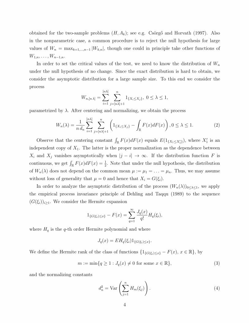
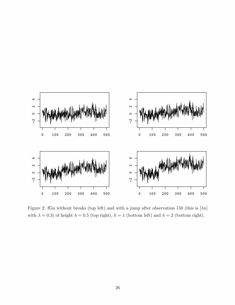
– Insert Figure 2 here –
In order to analyze how well the tests detect break points, we have introduced a level
18
shift h at time [nλ], i.e. we consider the time series
Xi =
{ξi for i = 1, . . . , [nλ]
ξi + h for i = [nλ] + 1, . . . , n.
We have done this for several choices of λ and h, for sample size n = 500. As Table 3 shows,
both tests detect breaks very well – and the better, the larger the level shift is and the more
in the middle the shift takes place. When the break occurs in the middle, both tests perform
equally well. Breaks at the beginning are better detected by the difference-of-means test.
– Insert Table 3 here –
5.2 Heavy-Tailed Data
In the second set of simulations, we took Pareto distributed data. Note that the Pareto(β, k)
distribution has distribution function
F (x) =
1−(kx
)βif x ≥ k
0 else,
where the scale parameter k is the smallest possible value for x and where β is a shape
parameter. The Pareto distribution has finite expected value when β > 1 and finite variance
when β > 2. The expected value and the variance are given by
µ = E(X) =βk
β − 1, β > 1
σ2 = Var(X) =βk2
(β − 1)2(β − 2), β > 2.
In order to obtain Pareto(β, k)-distributed X = G(ξ), we take G to be the quantile transform,
i.e. G(t) = k (Φ(t))−1/β where Φ denotes the standard normal distribution function, so that
for x ≥ k
P (Xi ≥ x) = P (G(ξi) ≥ x) = P(
(Φ(ξi))−1/β ≥ x
k
)= P
(ξi ≤ Φ−1(
(k
x
)β)
)=
(k
x
)β.
Since we want the Xi to be centered, we will in fact take
G(t) = k (Φ(t))−1/β − βk
β − 1. (25)
19
If we want Xi to be standardized to have mean 0 and variance 1, we will consider Z =
(X − µ)/σ and take
G(t) =
(βk2
(β − 1)2(β − 2)
)−1/2(k(Φ(t))−1/β − βk
β − 1
)(26)
The corresponding distribution function of Z is then
FZ(z) =
1−(
kσz+µ
)βif z ≥ k−µ
σ
0 else.(27)
and its density function is
fZ(z) =
{kββσ(σz + µ)−β−1 if z ≥ k−µ
σ
0 else(28)
Pareto(3, 1) Data: We first performed simulations with Pareto(3, 1) data, i.e. heavy-tailed
data with finite variance. In this case, β = 3, k = 1 and we have E(X) = 32
and Var(X) = 34.
For a better comparison with the simulations involving fractional Gaussian noise, we also
standardize the data, i.e. we consider (see (26)),
G(t) =1√3/4
((Φ(t))−1/3 − 3
2
).
The probability density function of the standardized X is given by (see (28)),
f(x) =
3√
34
(√34x+ 3
2
)−4if x ≥ −
√13
0 else.
G is again strictly decreasing, and by the above results, the Hermite rank of the class of
functions {I{G(ξi)≤x} − F (x), x ∈ R} is m = 1, the Hermite rank of G itself is m = 1 and
|∫R J1(x) dF (x)| = (2
√π)−1, see (20). Numerical integration yields
a1 = E[ξG(ξ)] =
√4
3
∫ ∞−∞
sΦ(s)−1/3ϕ(s) ds ≈ −0.6784.
Table 4 shows the observed level of the tests, for various sample sizes and various Hurst
parameters. For sample sizes up to n = 1, 000, the ”difference-of-means” test has level larger
than 10%. We conjecture that this is due to the slow convergence in Theorem 3. This
conjecture is supported by the outcomes of simulations with sample sizes n = 2, 000 and
n = 10, 000; see Table 4.
20
– Insert Table 4 here –
Table 5 gives the observed power of the ”difference-of-means” test and the Wilcoxon-
type test, for sample size n = 500 and various values of the break points and height of level
shift. The results show that the Wilcoxon-type test has larger power than the ”difference-of-
means” test for small level shift h, but that the ”difference-of-means” test outperforms the
Wilcoxon type test for larger level shifts.
– Insert Table 5 here –
However, the above comparison is not really meaningful, since the ”difference-of-means”
test has a realized level of approximately 10% while the Wilcoxon-type test has level close to
5%; see Table 4. Thus we have calculated the finite sample 5%-quantiles of the distribution
of the “difference-of-means” test, using a Monte-Carlo simulation; see Table 6. For example,
for n = 500 and H = 0.7, the corresponding critical value is 0.70. Thus we reject the null
hypothesis of no break point if the “difference-of-means” test statistic is greater than 0.70.
– Insert Table 6 here –
The value of 0.70 should be contrasted to the asymptotic (n = ∞) value of 0.59. To
obtain the asymptotic critical values, we proceeded as follows: according to Theorem 3,
the asymptotic distribution, under the null hypothesis, of the test statistic Dn equals the
distribution of
|a1| sup0≤λ≤1
|Z(λ)− λZ(1)|.
Thus the asymptotic upper α-quantiles of Dn can be calculated as |a1|qα, where qα is the
upper α-quantile of the distribution of sup0≤λ≤1 |Z(λ)− λZ(1)|, as tabulated in Table 1.
– Insert Table 7 here –
We have then calculated the power of the ”difference-of-means” test through simulation,
21
with n = 500, H = 0.7 and the finite sample quantile critical value of 0.70 rather than the
asymptotic value of 0.59 (see Table 6). Table 7 shows the power of the test. We can now
compare the results of the Wilcoxon-type test given in the right-hand side of Table 5 with the
finite sample “difference-of-means” test results given in Table 7. We see that the Wilcoxon-
type test has better power than the ”difference-of-means” test, except for large level shifts
at an early time. Such changes are detected more often by the ”difference-of-means” test.
Pareto(2, 1) Data: We now choose k = 1 and β = 2, so that the X have finite expectation,
but infinite variance. In order to have centered data, we take G as in (25), i.e.
G(t) =1√Φ(t)
− 2.
– Insert Table 8 here –
We will now compare both tests, i.e. the Wilcoxon-type test and the difference of means
test, although the latter can strictly speaking not be applied because it requires data with
finite variance, respectively G ∈ L2(R,N ). By Theorem 2, under the null hypothesis of no
change, the Wilcoxon-type test statistic Wn converges in distribution towards
1
2√π
sup0≤λ≤1
|Z1(λ)− λZ1(1)|.
In fact, as a consequence of Lemma 1, even the finite sample distribution of Wn is the same
as for normally distributed data. Table 8 gives the measured level of the Wilcoxon-type test
(the asymptotic level is 5%) and Table 9 suggests it has good power, especially for small
shifts in the middle of the observations.
– Insert Table 9 here –
Let us now consider the difference-of-means test. Note that, strictly speaking, Theorem 3
cannot be applied in the case of the Pareto data with β = 2 because it requires the variance
of the data to be finite. It is interesting nevertheless to use the asymptotic test suggested
by Theorem 3. Since G is strictly monotone, the Hermite rank of G is m = 1 as well, by the
22
remark following Theorem 3. Using numerical integration, we have calculated
a1 = E [ξG(ξ)] =
∫ ∞−∞
s(Φ(s)−1/2 − 2)ϕ(s) ds =
∫ ∞−∞
sΦ(s)−1/2ϕ(s) ds ≈ −1.40861.
We clearly see in Table 8 that the difference-of-means test very often falsely rejects the null
hypothesis, that is detects breaks where there are none, while the Wilcoxon-type test is
robust. Table 9 shows that both tests have good power, but again, the Wilcoxon tests is
clearly better, especially for small shifts in the middle of the observations.
6 Conclusion
We have investigated the properties of a nonparametric change-point test in the presence of
long-range dependent data. Our test is based on Wilcoxon’s two sample rank test statistic.
We analytically derive the asymptotic distribution of our test statistic, and we perform
a simulation study to calculate its power. The simulation study shows that already for
moderate sample sizes, our test attains the asymptotic level. For LRD Gaussian data, our
test has almost the same power as a difference-of-means test. For heavy-tailed data, our new
test outperforms the difference-of-means test. In a subsequent paper, we plan to derive the
asymptotic distribution of our test statistic under local alternatives.
Acknowledgement.
Herold Dehling and Aeneas Rooch were supported in part by the Collaborative Research
Grant 823, Project C3 Analysis of Structural Change in Dynamic Processes, of the German
Research Foundation. Murad S. Taqqu was supported in part by the NSF grants DMS-
0608669 and DMS-1007616 at Boston University. The authors wish to thank the referee of
this paper for his/her careful reading of the manuscript and for insightful and constructive
comments.
References
[1] Antoch, J., Huskova, M., Janic, M.A. & Ledwina, T. (2008). Data driven rank tests forthe change point problem. Metrika 68, 1–15.
[2] Aue, A., Hormann, S., Horvath, L. & Reimherr, M. (2009). Break detection in thecovariance structure of multivariate time series. The Annals of Statistics 37, 4046–4087.
[3] Berkes, I., Horvath, L., Kokoszka, P. & Shao, Q.-M. (2006). On discriminating betweenlong-range dependence and changes in the mean. The Annals of Statistics 34, 1140–1165.
23
[4] Csorgo, M. & Horvath, L. (1997). Limit Theorems in Change-Point Analysis. J. Wiley& Sons, Chichester.
[5] Dehling, H. & Fried, R. (2012). Asymptotic Distribution of Two-Sample EmpiricalU-Quantiles with Applications to Robust Tests for Shifts in Location. Journal of Mul-tivariate Analysis 105, 124–140.
[6] Dehling, H. & Taqqu, M.S. (1989). The empirical process of some long-range dependentsequences with an application to U-statistics. The Annals of Statistics 17, 1767–1783.
[7] Dehling, H. & Taqqu, M.S. (1991). Bivariate symmetric statistics of long-range depen-dent observations. Journal of Statistical Planning and Inference 28, 153–165.
[8] Giraitis, L., Leipus, R. & Surgailis, D. (1996). The change-point problem for dependentobservations. Journal of Statistical Planning and Inference 53, 297–310.
[9] Horvath, L. & Kokoszka, P. (1997). The effect of long-range dependence on change-pointestimators. Journal of Statistical Planning and Inference 64, 57–81.
[10] Kramer, W. & Sibbertsen, P. & Kleiber, C. (2002). Long memory versus structuralchange in financial time series. Allgemeines Statistisches Archiv 86, 83–96.
[11] Lehmann, E. (1975). Nonparametrics: Statistical Methods Based on Ranks. Holden-Day,San Francisco.
[12] Ling, S. (2007). Testing for change points in time series models and limiting theoremsfor NED sequences. The Annals of Statistics 35, 1213–1227.
[13] Shorack, G.R. & Wellner, J.A. (1986). Empirical Processes with Applications to Statis-tics. John Wiley & Sons, New York.
[14] Taqqu, M.S. (1979). Convergence of integrated processes of arbitrary Hermite rank.Zeitschrift fur Wahrscheinlichkeitstheorie und verwandte Gebiete 50, 53–83.
[15] Wang, L. (2003). Limit theorems in change-point problems with multivariate long-ranegdependent observations. Statistics & Decisions 21, 283–300.
[16] Wang, L. (2008a). Change-Point Detection with Rank Statistics in Long-Memory Time-Series Models. Australian & New Zealand Journal of Statistics 50, 241–256.
[17] Wang, L. (2008b). Change-in-mean problem for long memory time series models withapplications. Journal of Statistical Computation and Simulation 78, 653–668.
[18] Wied, D., Kramer, W. & Dehling, H. (2011). Testing for a change in correlation at anunknown point in time using an extended functional delta method. Econometric Theory,Available on CJO 2011 doi:10.1017/S0266466611000661.
Herold Dehling, Fakultat fur Mathematik, Ruhr-Universitat Bochum, Universitatsstraße 150,
44801 Bochum, Germany.
E-mail: [email protected]
24
0.0 0.5 1.0 1.5
0
0.5
1
1.5
2
0.0 0.5 1.0 1.5
0
0.5
1
Figure 1: Probability density (left) and distribution function (right) of sup0≤λ≤1 |Z(λ) −λZ(1)|; calculations based on 10, 000 simulation runs.
25
0 100 200 300 400 500
-2
02
4
0 100 200 300 400 500-2
02
4
0 100 200 300 400 500
-2
02
4
0 100 200 300 400 500
-2
02
4
Figure 2: fGn without breaks (top left) and with a jump after observation 150 (this is [λn]
with λ = 0.3) of height h = 0.5 (top right), h = 1 (bottom left) and h = 2 (bottom right).
26
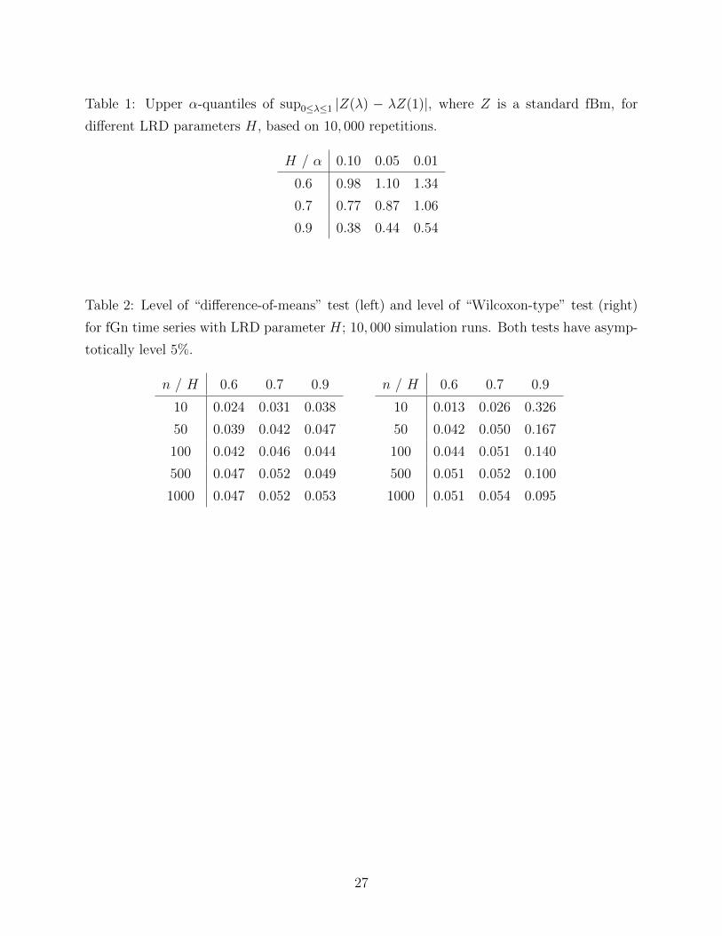
Table 1: Upper α-quantiles of sup0≤λ≤1 |Z(λ) − λZ(1)|, where Z is a standard fBm, for
different LRD parameters H, based on 10, 000 repetitions.
H / α 0.10 0.05 0.01
0.6 0.98 1.10 1.34
0.7 0.77 0.87 1.06
0.9 0.38 0.44 0.54
Table 2: Level of “difference-of-means” test (left) and level of “Wilcoxon-type” test (right)
for fGn time series with LRD parameter H; 10, 000 simulation runs. Both tests have asymp-
totically level 5%.
n / H 0.6 0.7 0.9
10 0.024 0.031 0.038
50 0.039 0.042 0.047
100 0.042 0.046 0.044
500 0.047 0.052 0.049
1000 0.047 0.052 0.053
n / H 0.6 0.7 0.9
10 0.013 0.026 0.326
50 0.042 0.050 0.167
100 0.044 0.051 0.140
500 0.051 0.052 0.100
1000 0.051 0.054 0.095
27
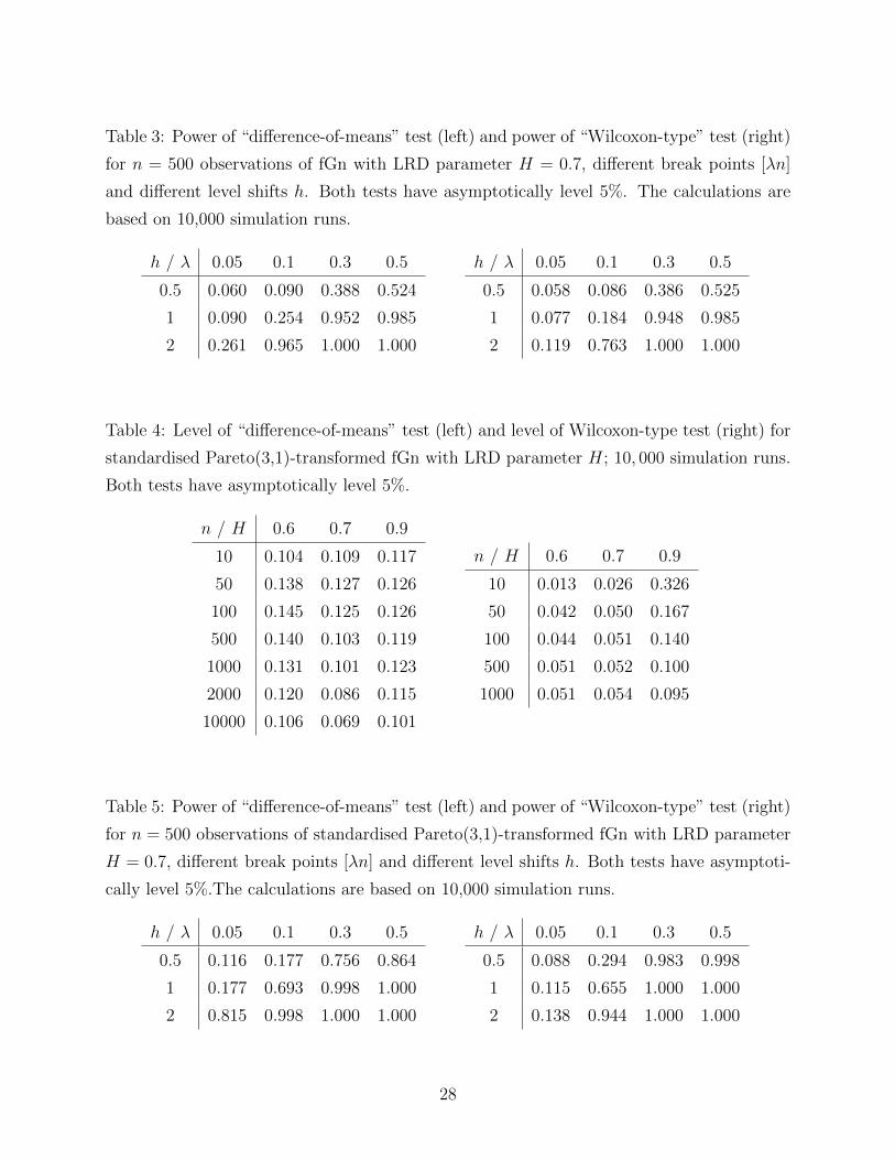
Table 3: Power of “difference-of-means” test (left) and power of “Wilcoxon-type” test (right)
for n = 500 observations of fGn with LRD parameter H = 0.7, different break points [λn]
and different level shifts h. Both tests have asymptotically level 5%. The calculations are
based on 10,000 simulation runs.
h / λ 0.05 0.1 0.3 0.5
0.5 0.060 0.090 0.388 0.524
1 0.090 0.254 0.952 0.985
2 0.261 0.965 1.000 1.000
h / λ 0.05 0.1 0.3 0.5
0.5 0.058 0.086 0.386 0.525
1 0.077 0.184 0.948 0.985
2 0.119 0.763 1.000 1.000
Table 4: Level of “difference-of-means” test (left) and level of Wilcoxon-type test (right) for
standardised Pareto(3,1)-transformed fGn with LRD parameter H; 10, 000 simulation runs.
Both tests have asymptotically level 5%.
n / H 0.6 0.7 0.9
10 0.104 0.109 0.117
50 0.138 0.127 0.126
100 0.145 0.125 0.126
500 0.140 0.103 0.119
1000 0.131 0.101 0.123
2000 0.120 0.086 0.115
10000 0.106 0.069 0.101
n / H 0.6 0.7 0.9
10 0.013 0.026 0.326
50 0.042 0.050 0.167
100 0.044 0.051 0.140
500 0.051 0.052 0.100
1000 0.051 0.054 0.095
Table 5: Power of “difference-of-means” test (left) and power of “Wilcoxon-type” test (right)
for n = 500 observations of standardised Pareto(3,1)-transformed fGn with LRD parameter
H = 0.7, different break points [λn] and different level shifts h. Both tests have asymptoti-
cally level 5%.The calculations are based on 10,000 simulation runs.
h / λ 0.05 0.1 0.3 0.5
0.5 0.116 0.177 0.756 0.864
1 0.177 0.693 0.998 1.000
2 0.815 0.998 1.000 1.000
h / λ 0.05 0.1 0.3 0.5
0.5 0.088 0.294 0.983 0.998
1 0.115 0.655 1.000 1.000
2 0.138 0.944 1.000 1.000
28
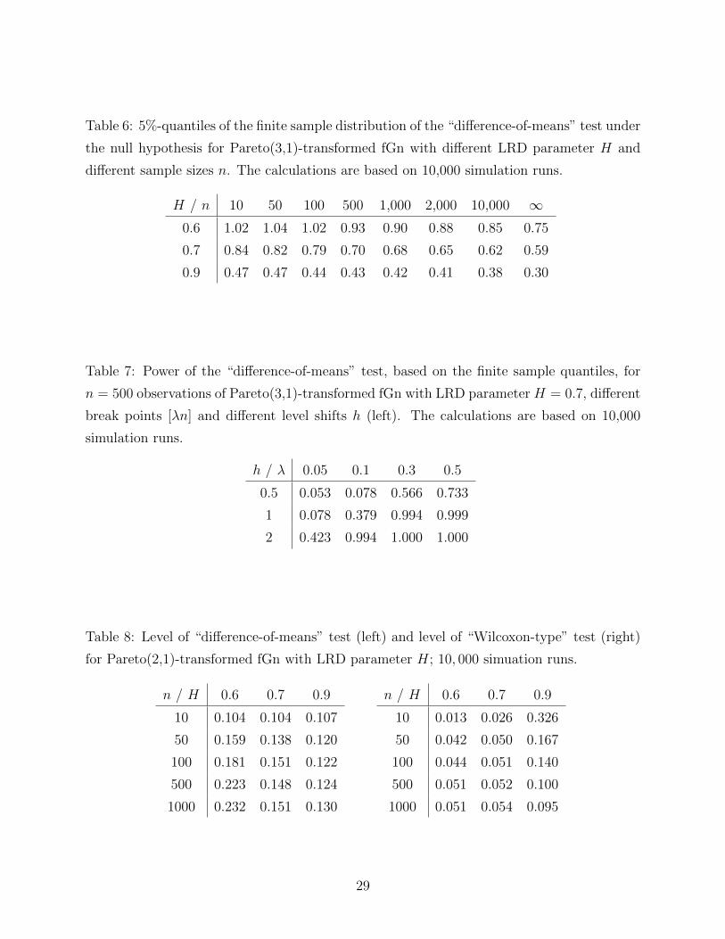
Table 6: 5%-quantiles of the finite sample distribution of the “difference-of-means” test under
the null hypothesis for Pareto(3,1)-transformed fGn with different LRD parameter H and
different sample sizes n. The calculations are based on 10,000 simulation runs.
H / n 10 50 100 500 1,000 2,000 10,000 ∞0.6 1.02 1.04 1.02 0.93 0.90 0.88 0.85 0.75
0.7 0.84 0.82 0.79 0.70 0.68 0.65 0.62 0.59
0.9 0.47 0.47 0.44 0.43 0.42 0.41 0.38 0.30
Table 7: Power of the “difference-of-means” test, based on the finite sample quantiles, for
n = 500 observations of Pareto(3,1)-transformed fGn with LRD parameter H = 0.7, different
break points [λn] and different level shifts h (left). The calculations are based on 10,000
simulation runs.
h / λ 0.05 0.1 0.3 0.5
0.5 0.053 0.078 0.566 0.733
1 0.078 0.379 0.994 0.999
2 0.423 0.994 1.000 1.000
Table 8: Level of “difference-of-means” test (left) and level of “Wilcoxon-type” test (right)
for Pareto(2,1)-transformed fGn with LRD parameter H; 10, 000 simuation runs.
n / H 0.6 0.7 0.9
10 0.104 0.104 0.107
50 0.159 0.138 0.120
100 0.181 0.151 0.122
500 0.223 0.148 0.124
1000 0.232 0.151 0.130
n / H 0.6 0.7 0.9
10 0.013 0.026 0.326
50 0.042 0.050 0.167
100 0.044 0.051 0.140
500 0.051 0.052 0.100
1000 0.051 0.054 0.095
29
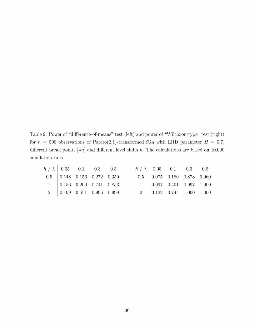
Table 9: Power of “difference-of-means” test (left) and power of “Wilcoxon-type” test (right)
for n = 500 observations of Pareto(2,1)-transformed fGn with LRD parameter H = 0.7,
different break points [λn] and different level shifts h. The calculations are based on 10,000
simulation runs.
h / λ 0.05 0.1 0.3 0.5
0.5 0.148 0.156 0.272 0.350
1 0.156 0.200 0.741 0.853
2 0.199 0.651 0.996 0.999
h / λ 0.05 0.1 0.3 0.5
0.5 0.075 0.180 0.878 0.960
1 0.097 0.401 0.997 1.000
2 0.122 0.744 1.000 1.000
30
Recommended


![Bayesian nonparametric mean residual life regressionarXiv:1412.0367v2 [stat.AP] 5 Nov 2018 survival times. KEYWORDS: Dependent Dirichlet process, Dirichlet process mixture models,](https://img.pdfslide.us/doc/110x75/60c2a6848928e11b25203e25/bayesian-nonparametric-mean-residual-life-regression-arxiv14120367v2-statap.jpg)