Nonlinear Equations
W. E. Schiesser
Iacocca D307
111 Research Drive
Lehigh University
Bethlehem, PA 18015
(610) 758-4264 (o�ce)
(610) 758-5057 (fax)
http://www.lehigh.edu/~wes1/wes1.html
1

Nonlinear Equations
http://www.lehigh.edu/~wes1/apci/24feb00-b.ps
http://www.lehigh.edu/~wes1/apci/24feb00-b.pdf
http://www.lehigh.edu/~wes1/apci/24feb00-s.tex
http://www.lehigh.edu/~wes1/apci/24feb00-s.ps
http://www.lehigh.edu/~wes1/apci/24feb00-s.pdf
Previous lectures are in:
http://www.lehigh.edu/~wes1/apci/28jan00.tex
http://www.lehigh.edu/~wes1/apci/28jan00.ppt
http://www.lehigh.edu/~wes1/apci/28jan00.ps
http://www.lehigh.edu/~wes1/apci/28jan00.pdf
http://www.lehigh.edu/~wes1/apci/18feb00.ps
http://www.lehigh.edu/~wes1/apci/18feb00.pdf
A Table of Contents is in:
http://www.lehigh.edu/~wes1/apci/�les.txt
1. Newton's method and quasilinearization (WES)
2. Obtaining derivatives (LTB)
3. Broyden's method (LTB)
4. Continuation methods (WES)
5. Davidenko's equation (WES)
2

6. Levenberg-Marquardt method (WES)
7. Tearing algorithms (LTB)
8. Direct substitution (LTB)
9. Wegstein method (LTB)
10. References and software (LTB/WES)
3

The General NonlinearProblem
The n x n nonlinear problem is:
f1(x1; x2; � � � ; xn) = 0
f2(x1; x2; � � � ; xn) = 0...
fn(x1; x2; � � � ; xn) = 0
(1)
which can be summarized as
f(x) = 0 (2)
where we use bold face to denote vectors:
f =
26664
f1f2...
fn
37775 ;x =
26664
x1x2...
xn
37775 ; 0 =
26640
0
0
0
3775
Two points:
� Nonlinear equations are generally solved numerically by the iterative
solution of linear equations
� John Rice states (approximately) that the solution of nonlinear equa-
tions is the most di�cult problem in scienti�c computation
4

Newton's Method andQuasilinearization
To obtain a form of Newton's method for systems of equations, we start with
the Taylor series in n variables, e.g., n = 2, we want to obtain the values of
x1; x2 that satisfy the 2 x 2 system
f1(x1; x2) = 0
f2(x1; x2) = 0(7)
If f1 and f2 are expanded in two Taylor series in two dimensions (with respect
to the iteration counter k)
f1(xk+11 ; xk+1
2 ) = f1(xk
1; xk
2) +@f1(x
k
1; xk
2)
@x1(xk+1
1 � xk1) +@f1(x
k
1; xk
2)
@x2(xk+1
2 � xk2) + � � �
f2(xk+11 ; xk+1
2 ) = f2(xk
1; xk
2) +@f2(x
k
1; xk
2)
@x1(xk+1
1 � xk1) +@f2(x
k
1; xk
2)
@x2(xk+1
2 � xk2) + � � �
(8)
truncation after the �rst derivative terms, with the resulting equations ex-
pressed in terms of Newton corrections
�xk1 = (xk+11 � xk1)
�xk2 = (xk+12 � xk2)
and with just the right Newton corrections so that the LHS's of eqs. (8) are
zero, gives
@f1(xk
1; xk
2)
@x1�xk1 +
@f1(xk
1; xk
2)
@x2�xk2 = �f1(x
k
1; xk
2)
@f2(xk
1; xk
2)
@x1�xk1 +
@f2(xk
1; xk
2)
@x2�xk2 = �f2(x
k
1; xk
2)
(9)
Eqs. (9) are a 2 x 2 linear system in the two Newton corrections, �xk1 ;�xk2then can be solved by any standard method for linear equations, e.g., Gauss
row reduction. The unknowns can then be updated iteratively by
5

xk+11 = �xk1 + xk1
xk+12 = �xk2 + xk2
k = 0; 1; 2; � � � (10)
Eq. (9) can be generalized to the n x n case by writing it in matrix form
J�x = �f (11)
where
J =
2666666664
@f1(xk
1; xk
2; � � � ; xk
n)
@x1
@f1(xk
1; xk
2; � � � ; xk
n)
@x2� � �
@f1(xk
1; xk
2; � � � ; xk
n)
@xn@f2(x
k
1; xk
2; � � � ; xk
n)
@x1
@f2(xk
1; xk
2; � � � ; xk
n)
@x2� � �
@f2(xk
1; xk
2; � � � ; xk
n)
@xn...
.... . .
...
@fn(xk
1; xk
2; � � � ; xk
n)
@x1
@fn(xk
1; xk
2; � � � ; xk
n)
@x2� � �
@fn(xk
1; xk
2; � � � ; xk
n)
@xn
3777777775;�x =
26664
�xk1�xk2...
�xkn
37775
(12)(13)
Eq. (11) is Newton's method for an n x n system (a remarkably compact
and useful equation).
We now consider three small nonlinear problems:
(1) The third order polynomial
f(x) = x3 � 2x� 5 = 0
As noted on 28jan00, this polynomial may be the �rst application of Newton's
method, since Newton used it to illustrate his method
If we apply Newton's method, eq. (9), for the scalar (n = 1) case
df(xk)
dx(xk+1
� xk) = �f(xk)
6

or the familiar form
xk+1 = xk �f(xk)
df(xk)=dx; k = 0; 1; � � �
where k is an iteration index or counter.
We can make some observations about the application of Newton's method
to Newton's polynomial and the generalization of Newton's method to the n
x n problem (eq. (11)):
� The polynomial has three roots (three reals or one real and two complex
conjugates - conjugates are required for the polynomial to have real
coe�cients). This conclusion is from a famous proof by C. F. Gauss;
in general, nonlinear problems will have multiple (nonunique) roots.
� If we make the choice of the initial starting point at a root of
df(x)
dx= 3x2 � 2 = 0
or
x0 = �
p2=3
the method will fail because this is a singular point (the Jacobian ma-
trix, or in this case, the �rst derivative, is singular).
� Also, if we choose a starting point near the singular point, the method
will most likely fail, i.e., the system is near-singular (this is clear if we
consider Newton's method as a projection along the tangent to f(x)).
7

� The choice of an initial point that is not singular or near-singular be-
comes increasingly di�cult as the size of the problem increases (more
equations), and we should have a test in our software for the condition
of the Jacobian matrix.
� The Jacobian matrix, J (in eq. (11)), is n x n, and therfore grows
quickly with the problem size.
� The Jacobian matrix is not constant (a property of nonlinear systems),
and therefore must be updated as the iterations proceed; updating
at every iteration may not be required since all that is required is
convergence of the iterations.
� The right hand side (RHS) vector, f in eq. (11), must also be updated as
the iterations proceed, but this will be less costly than for the Jacobian
matrix because of the smaller size of f .
� A stopping criterion is required for the iterations, e.g.,
���xki
�� < "i; i = 1; 2; � � � ; n (relative or absolute)
���xk+1i
��xki
�� < "i; i = 1; 2; � � � ; n (relative or absolute)
��fi(xki )�� < "i; i = 1; 2; � � � ; n
��fi(xk+1i
)� fi(xk
i)�� < "i; i = 1; 2; � � � ; n
� Quasilinearization is the characterization of eq. (11) denoting the lin-
earization with respect to the iteration index or counter, k.
8
� Eq. (11) is almost never solved as
�x = �J�1f
Rather, J is factored (LU, QR factorization), and eq. (11) is then solved
as a system of linear algebraic equations (for the vector of Newton
corrections �x).
� For large nonlinear systems, e.g., n > 100, the structure of the Jacobian
matrix in eq. (11) can often be exploited to good advantage, e.g., as a
banded or sparse matrix.
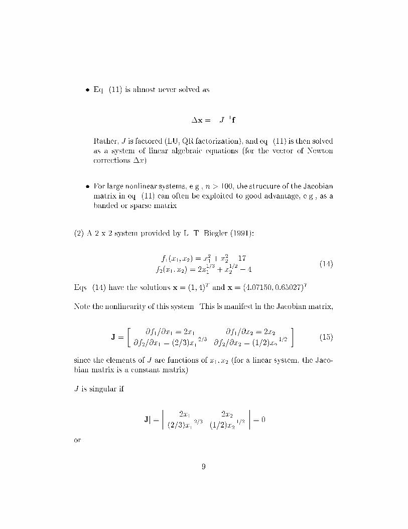
(2) A 2 x 2 system provided by L. T. Biegler (1991):
f1(x1; x2) = x21 + x22 � 17
f2(x1; x2) = 2x1=31 + x
1=22 � 4
(14)
Eqs. (14) have the solutions x = (1; 4)T and x = (4:07150; 0:65027)T .
Note the nonlinearity of this system. This is manifest in the Jacobian matrix,
J =
�@f1=@x1 = 2x1 @f1=@x2 = 2x2
@f2=@x1 = (2=3)x�2=31 @f2=@x2 = (1=2)x
�1=22
�(15)
since the elements of J are functions of x1; x2 (for a linear system, the Jaco-
bian matrix is a constant matrix).
J is singular if
jJj =
���� 2x1 2x2
(2=3)x�2=31 (1=2)x
�1=22
���� = 0
or
9

(2x1) (1=2)x�1=22 � (2x2) (2=3)x
�2=31 = 0 (16)
Eq. (16) is a relationship between x1 and x2 that de�nes a locus of singular
points for system (14). Later we will start a numerical solution at a singular
point given by eq. (16) and observe what happens with the calculation of
the solution.
Applying eq. (11) to eqs. (14), we have
�2x1 2x2
(2=3)x�2=31 (1=2)x
�1=22
�k ��x1�x2
�k= �
�x21 + x22 � 17
2x1=31 + x
1=22 � 4
�k
or
2xk1�xk1 + 2xk2�xk2 = �(xk1)2� (xk2)
2 + 17
(2=3)(xk1)�2=3�xk1 + (1=2)(xk2)
�1=2�xk2 = �2(xk1)1=3� (xk2)
1=2 + 4(17)
A basic algorithm for solving eqs. (14) is therefore
1 Select xk1 = x01; xk
2 = x022 Substitute xk1; x
k
2 in eqs. (17)
3 Solve eqs. (17) for �xk1;�xk24���xk1
�� < "1 and���xk2
�� < "2 ?; yes - output, quit; no - continue
5 xk+11 = xk1 +�xk1 ; x
k+12 = xk2 +�xk2
6 Let xk1 = xk+11 ; xk2 = xk+1
2 ; go to 2
Note that all that is required to implement this algorithm is a linear equation
solver (to compute the Newton corrections, �xk1;�xk2).
(3) A 4 x 4 system from Riggs, J. B. (1994), \An Introduction to Numerical
Methods for Chemical Engineers", 2nd ed., Texas Tech University Press, pp
82-89:
A continuous stirred tank reactor (CSTR) is used for the following reaction
scheme
10

Ar1! 2B
Ar2
�r3
C
Br4! C +D
where
r1 = k1CA
r2 = k2C3=2
A
r3 = k3C2C
r4 = k4C2B
k1 = 1:0 sec�1
k2 = 0:2 liter1=2/gm mol1=2-sec
k3 = 0:05 liter/gm mol-sec
k4 = 0:4 liter/gm mol-sec
Each reaction rate (r1 to r4) is in gm mols/liter-sec. If the volume of the
reactor is Vr = 100 liters, the volumetric ow rate through the reactor is
Q = 50 liters/sec, and the feed to the reactor is CA0 = 1:0 gm mol/liter, the
steady state material balances for the reactor are:
f1(CA; CB; CC ; CD) = �QCA +QCA0 + VR(�k1CA � k2C3=2
A+ k3C
2C) = 0
(17a)
f2(CA; CB; CC; CD) = �QCB + VR(2k1CA � k4C2B) = 0 (17b)
f3(CA; CB; CC ; CD) = �QCC + VR(k2C3=2
A� k3C
2C+ k4C
2B) = 0 (17c)
11

f4(CA; CB; CC ; CD) = �QCD + VR(k4C2B) = 0 (17d)
We will subsequently consider a solution to eqs. (17) to three signi�cant
�gures, i.e., the values of CA; CB; CC ; CD that satisfy eqs. (17).
One possible approach to computing a solution would be to convert eqs. (17)
to a system of ordinary di�erential equations (ODEs):
VdCA
dt= �QCA +QCA0 + VR(�k1CA � k2C
3=2
A+ k3C
2C) = 0; CA(0) = C0
A
(18a)
VdCB
dt= �QCB + VR(2k1CA � k4C
2B) = 0; CB(0) = C0
B(18b)
VdCC
dt= �QCC + VR(k2C
3=2
A� k3C
2C+ k4C
2B) = 0; CC(0) = C0
C(18c)
VdCD
dt= �QCD + VR(k4C
2B) = 0; CD(0) = C0
D(18d)
where: (a) V is the volume of the reactor (if we are interested in the true
dynamic response of the CSTR) or (b) V is a \pseudo" time constant if all
we are interested in is the �nal steady state withdCA
dt�
dCB
dt�
dCC
dt�
dCD
dt� 0.
Method (b) is a perfectly satisfactory way of solving eqs. (14) called the
method of \false transients". However, care must be given to adding the
derivatives to the nonlinear equations with the correct sign to ensure a stable
steady state or equilibrium solution (which may not be obvious for large
systems of equations). Later we will consider a systematic procedure for
adding the derivatives.
12

Continuation Methods
Consider again the 2 x 2 system of eq. (7). If we assume two related functions,
g1(x1; x2)
g2(x1; x2)
with known solutions based on arbitrary values x1 = x01; x2 = x02;i.e.,
g1(x01; x
02) = 0
g2(x01; x
02) = 0
then we can form a vector of homotopy functions
h1(x1; x2; t) = tf1(x1; x2) + (1� t)g1(x1; x2)
h2(x1; x2; t) = tf2(x1; x2) + (1� t)g2(x1; x2)(19)
where t is an embedded homotopy continuation parameter.
Now we vary t over the interval 0 � t � 1 while always setting the homotopy
functions to zero. This can be easily visualized using a table
13

t h1(x1; x2; t) = 0 x1;x2 Comments
h2(x1; x2; t) = 0
0 g1(x1; x2) = 0 x01 Assumed initial
g2(x1; x2) = 0 x02 solution
0:1 0:1f1(x1; x2) + 0:9g1(x1; x2) = 0 x0:11 x0:11 close to x010:1f2(x1; x2) + 0:9g2(x1; x2) = 0 x0:12 x0:12 close to x02
0:2 0:2f1(x1; x2) + 0:8g1(x1; x2) = 0 x0:21 Root �nder required
0:2f2(x1; x2) + 0:8g2(x1; x2) = 0 x0:22 at each step
0:3 0:3f1(x1; x2) + 0:7g1(x1; x2) = 0 x0:31
0:3f2(x1; x2) + 0:7g2(x1; x2) = 0 x0:32
......
...
0:9 0:9f1(x1; x2) + 0:9g1(x1; x2) = 0 x0:91
0:9f2(x1; x2) + 0:9g2(x1; x2) = 0 x0:92
1 f1(x1; x2) = 0 x11 Required solution
f2(x1; x2) = 0 x12
The essential features of this continuation method are:
� The solution is continued from the known solution
� The closer g1(x1; x2) and g1(x1; x2) are to f1(x1; x2) and f2(x1; x2), the
better chances of this procedure working.
� However, the success of the method is generally not particularly sensi-
tive to the selection of g1(x1; x2) and g1(x1; x2). For example, we could
try linear functions
14
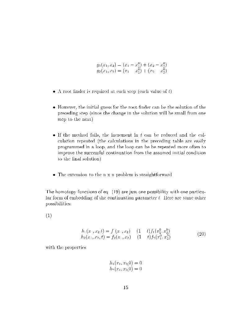
g1(x1; x2) = (x1 � x01) + (x2 � x02)
g2(x1; x2) = (x1 � x01) + (x2 � x02)
� A root �nder is required at each step (each value of t).
� However, the initial guess for the root �nder can be the solution of the
preceding step (since the change in the solution will be small from one
step to the next).
� If the method fails, the increment in t can be reduced and the cal-
culation repeated (the calculations in the preceding table are easily
programmed in a loop, and the loop can be be repeated more often to
improve the successful continuation from the assumed initial condition
to the �nal solution).
� The extension to the n x n problem is straightforward.
The homotopy functions of eq. (19) are just one possibility with one particu-
lar form of embedding of the continuation parameter t. Here are some other
possibilities:
(1)
h1(x1; x2;t) = f1(x1; x2)� (1� t)f1(x01; x
02)
h2(x1; x2; t) = f2(x1; x2)� (1� t)f2(x01; x
02)
(20)
with the properties
h1(x1; x2;0) = 0
h2(x1; x2;0) = 0
15

h1(x1; x2;1) = f1(x1; x2)
h2(x1; x2; 1) = f2(x1; x2)
as required.
(2)
h1(x1; x2;t) = f1(x1; x2)� e�tf1(x01; x
02)
h2(x1; x2; t) = f2(x1; x2)� e�tf2(x01; x
02)
(21)
with the properties
h1(x1; x2;0) = 0
h2(x1; x2;0) = 0
h1(x1; x2;1) = f1(x1; x2)
h2(x1; x2;1) = f2(x1; x2)
as required (note that the interval in t is now 0 � t � 1).
16

Davidenko's Equation
If we consider again the embedding of eqs. (21), we can analyze it by con-
sidering the di�erentials of the homotopy functions
dh1 =@h1
@x1dx1 +
@h1
@x2dx2 +
@h1
@tdt = 0
dh2 =@h2
@x1dx1 +
@h2
@x2dx2 +
@h2
@tdt = 0
(22)
(these di�erentials are zero since h1(x1; x2; t) = 0; h2(x1; x2; t) = 0). From
eqs. (21) and (22), we have
dh1 =@f1
@x1dx1 +
@f1
@x2dx2 + e�tf1(x
01; x
02)dt = 0
dh2 =@f2
@x1dx1 +
@f2
@x2dx2 + e�tf2(x
01; x
02)dt = 0
or
@f1
@x1
dx1
dt+
@f1
@x2
dx2
dt= �e�tf1(x
01; x
02) = �f1(x1; x2)
@f2
@x1
dx1
dt+
@f2
@x2
dx2
dt= �e�tf2(x
01; x
02) = �f2(x1; x2)
(23)
Eqs. (23), a di�erential form of Newton's method, are the Davidenko di�er-
ential equation, that can be written in matrix form for the n x n problem
as
Jdx
dt= �f (24)
where again J and f are the Jacobian matrix and function vector of the
nonlinear system, respectively, anddx
dtis the derivative of the solution vector
with respect to the continuation parameter, t (compare eq. (11) with eq. (24)
to see why Davidenko's ODE is a di�erential form of Newton's method).
17

Eq. (24) de�nes an initial value problem, requiring an initial condition vector
that serves as the assumed initial or starting solution
x(0) = x0 (25)
The procedure for the solution of the nonlinear system is to integrate eq.
(24) until
Jdx
dt� 0 which implies f � 0 (26)
This is the required solution of the nonlinear system, i.e., whatever the so-
lution vector, x(t); of eq. (24) is when condition (26) occurs is the required
solution of the original nonlinear system.
Note that form of ODEs (23); there is more than one derivative in each ODE,
and they are termed linearly implicit ODEs. Special integrators are available
for ODEs of this form, e.g., LSODI, DASSL.
Since eqs. (23) are linear in the derivatives, another approach to integrating
them is �rst use a linear algebraic equation solver to compute the derivative
vector,dx
dt; then use a conventional ODE integrator for the explicit ODEs to
compute a solution. In other words, eq. (24) can be written as
dx
dt= �J�1f (27)
This method works well for relatively low order systems.
The advantages of using eq. (24) or eq. (27) relative to the conventional
�nite stepping Newton method, eq. (11), are
� The solution of eqs. (24) or (27) proceeds by di�erential steps rather
than the �nite steps of Newton's method. Thus, the convergence to
a solution is often more reliable, i.e., Davidenko's method may work
when Newton's method fails.
18

� In other words, we are relying on the error monitoring and step size con-
trol of an ODE integrator (rather than the use of damping in Newton's
method).
� The implementation of eq. (24) requires only an integrator for linearly
implicit ODEs, e.g., LSODI, DASSL.
� Eq. (27) requires only a linear equation solver plus an integrator for
explicit ODEs.
Thus, the di�erential approach to Newton's method can be implemented with
readily available software.
To conclude this section, consider the application of eqs. (24) and (27) to
problem (2). For eq. (24)
�2x1 2x2
(2=3)x�2=31 (1=2)x
�1=22
�26664
dx1
dt
dx2
dt
37775 = �
�x21 + x22 � 17
2x1=31 + x
1=22 � 4
�
or
2x1dx1
dt+ 2x2
dx2
dt= � (x21 + x22 � 17)
(2=3)x�2=31
dx1
dt+ (1=2)x
�1=22
dx2
dt= �
�2x
1=31 + x
1=22 � 4
� (28)
For eq. (27)
26664
dx1
dt
dx2
dt
37775 = �
�2x1 2x2
(2=3)x�2=31 (1=2)x
�1=22
��1 �
x21 + x22 � 17
2x1=31 + x
1=22 � 4
�(29)
A Fortran program for the solution of eqs. (29) is given in Schiesser (1994),
pp 174-193.
19

Finally, we can analyze the convergence of solutions to Davidenko's ODE,
eq. (24). For the scalar case, eq. (24) becomes
df
dx
dx
dt= �f
which rearranges to
df
f= �dt
Integration of each side of this ODE, subject to the initial condition
f(t0) = f0
gives
ln(f=f0) = �(t� t0)
or
f = f0e�(t�t0) (30)
Eq. (30) indicates that the convergence of Davidenko's method is exponen-
tial in t. This result also carries over to the n x n case. This exponential
convergence is demonstrated numerically for problem (2) in Schiesser (1994).
20

Levenberg-Marquardt Method
A major di�culty with Newton's method, eq. (11), or Davidenko's method,
eq. (24), is failure caused by a singular or near singular Jacobian matrix (note
that both methods require the inverse Jacobian matrix). To circumvent this
problem, we consider the discrete and di�erential (continuous) Levenberg-
Marquardt methods:
�(1� �)JTJ + �I
�x = �JT f (31)
�(1� �)JTJ + �I
dxdt
= �JT f (32)
When � = 0;eqs. (31) and (32) reduce to
JTJ�x = �JT f or J�x = �f (33)
JTJdx
dt= �JT f or J
dx
dt= �f (34)
Eqs. (33) and (34) are just Newton's method and Davidenko's method,
respectively (and both will fail if J is singular).
When � = 1;eqs. (31) and (32) reduce to
�x = �JT f (35)
dx
dt= �JT f (36)
Eqs. (35) and (36) express the discrete and di�erential steepest descent. Note
that neither eq. (35) nor eq. (36) requires the inverse Jacobian. However,
these equations re ect the conditions for a maximum or minimum in
21

ss =
NXi
f 2i
(37)
Thus, eqs. (35) and (36) can \get stuck" at a local maximum or minimum of
ss of eq. (37). Also, when they do approach the solution f1 = f2 = � � � fN =
0, they do so relatively slowly (compared to Newton's method).
Therefore, the approach to avoiding a singular system and still approach the
solution f1 = f2 = � � � fN = 0; is to use 0 < � < 1, and to possibly vary � as
the solution proceeds by monitoring the condition of J:
Equations (31) and (32) have been coded in library software. In particular,
eq. (32) is available as a Fortran program from WES. We conclude this
discussion with the application of eq. (32) to problem (3).
The initial conditions for eq. (32) are
C...
C... First starting point
IF(NORUN.EQ.1)THEN
X(1)=0.5D0
X(2)=0.5D0
X(3)=0.5D0
X(4)=0.5D0
END IF
C...
C... LM parameter in eq. (1). Note: the calculation fails with
C... L = 0 for a singular system (determinant of the Jacobian
C... matrix is zero)
L=0.5D0
The programming of the RHS of eqs. (32) is then
C...
22

C... Once past the singular point, the DLM parameter is reset to
C... zero to give the differential Newton's method (and thereby
C... enhance the rate of convergence)
IF(T.GT.1.0D0)L=0.0D0
C...
C... Vector of functions (f in eq. (1))
CALL FUNC(N,X,F)
C...
C... Jacobian matrix (J in eq. (1))
CALL JAC(N,X,J)
C... T
C... Jacobian matrix transpose (J in eq. (1))
CALL TRANS(N,J,JT)
C...
C... T
C... Matrix product (J*J in eq. (1))
CALL MULT(N,N,N,J,JT,JTJ)
C... T
C... Left hand side coupling matrix (1-L)*J*J + L*I in eq. (1))
CALL CMAT(N,JTJ,L,ID,JTJPLI)
C...
C... T
C... Right hand side vector (-J*f in eq. (1))
CALL MULT1(N,N,1,JT,F,JTF)
C...
C... Solve for the vector of derivatives, dx/dt, in eq. (1) (in
C... effect, eq. (1) is premultiplied by the inverse of the LHS
C... coupling matrix). DECOMP performs an LU decomposition and
C... computes the condition number of JTJPLI
CALL DECOMP(N,N,JTJPLI,COND,IPVT,WORK)
C...
C... Compute derivative vector dx/dt from JTJPLI with RHS JTF,
C... i.e., solve eq. (1) for dx/dt. The solution is returned
C... in JTF
CALL SOLVE(N,N,JTJPLI,JTF,IPVT)
C...
C... Transfer array JTF to array DXDT so the derivative vector,
C... dx/dt, is available in COMMON/F/ for the ODE integrator
23

DO 2 I=1,N
DXDT(I)=JTF(I,1)
2 CONTINUE
RETURN
END
The programming of the function vector is
SUBROUTINE FUNC(N,X,F)
C...
C... Subroutine FUNC computes the vector of functions,
C... -f, in eq. (1) (note the minus sign, as required
C... in the RHS of eq. (1))
C...
C... Arguments
C...
C... N order of the NLE system (number of NLE)
C... (input)
C...
C... X solution vector of size N (input)
C...
C... F function vector of size N (output)
C...
IMPLICIT DOUBLE PRECISION(A-H,O-Z)
DIMENSION X(N), F(N)
C...
C... COMMON area for the problem parameters
COMMON/P/ VR, Q, CA0, RK1, RK2, RK3, RK4
C...
C... Problem variables
CA=X(1)
CB=X(2)
CC=X(3)
CD=X(4)
C...
C... Function vector
F(1)=-CA+VR*(-RK1*CA-RK2*CA**1.5D0+RK3*CC**2)/Q+CA0
24

F(2)=-CB+VR*(2.0D0*RK1*CA-RK4*CB**2)/Q
F(3)=-CC+VR*(RK2*CA**1.5D0-RK3*CC**2+RK4*CB**2)/Q
F(4)=-CD+VR*(RK4*CB**2)/Q
C...
C... Reverse the sign of the function vector in accordance
C... with the RHS of eq. (1)
DO 1 I=1,N
F(I)=-F(I)
1 CONTINUE
RETURN
END
The programming of the Jacobian matrix is:
SUBROUTINE JAC(N,X,J)
C...
C... Subroutine JAC computes the Jacobian matrix
C... of the vector of functions, f, in eq. (1)
C... (note the elements of J are computed for f,
C... not -f)
C...
C... Arguments
C...
C... N order of the NLE system (number of NLE)
C... (input)
C...
C... X solution vector of size N (input)
C...
C... J Jacobian matrix of size N x N (output)
C...
IMPLICIT DOUBLE PRECISION(A-H,O-Z)
DOUBLE PRECISION J
DIMENSION X(N), J(N,N)
C...
C... COMMON area for the problem parameters
COMMON/P/ VR, Q, CA0, RK1, RK2, RK3, RK4
C...
25

C... Problem variables
CA=X(1)
CB=X(2)
CC=X(3)
CD=X(4)
C...
C... Jacobian matrix
J(1,1)=-1.0D0+VR*(-RK1-1.5D0*RK2*CA**0.5)/Q
J(1,2)=0.0D0
J(1,3)=VR*(2.0D0*RK3*CC)/Q
J(1,4)=0.0D0
J(2,1)=VR*(2.0D0*RK1)/Q
J(2,2)=-1.0D0+VR*(-2.0D0*RK4*CB)/Q
J(2,3)=0.0D0
J(2,4)=0.0D0
J(3,1)=VR*(1.5D0*RK2*CA**0.5D0)/Q
J(3,2)=VR*(2.0D0*RK4*CB)/Q
J(3,3)=-1.0D0+VR*(-2.0D0*RK3*CC)/Q
J(3,4)=0.0D0
J(4,1)=0.0D0
J(4,2)=VR*(2.0D0*RK4*CB)/Q
J(4,3)=0.0D0
J(4,4)=-1.0D0
RETURN
END
The output from the complete program is:
RUN NO. - 1 Four component, steady state CSTR
equations
INITIAL T - 0.000D+00
FINAL T - 0.200D+03
PRINT T - 0.500D+02
26

NUMBER OF DIFFERENTIAL EQUATIONS - 4
INTEGRATION ALGORITHM - LSODES
MAXIMUM INTEGRATION ERROR - 0.100D-06
1
t = 0.0
Ca = 0.50000 dCa/dt = -0.416D+01 res f1 = 0.616D+00
Cb = 0.50000 dCb/dt = -0.261D+01 res f2 = -0.130D+01
Cc = 0.50000 dCc/dt = -0.176D+01 res f3 = 0.184D+00
Cd = 0.50000 dCd/dt = -0.122D+01 res f4 = 0.300D+00
t = 50.0
Ca = 0.31814 dCa/dt = 0.120D-03 res f1 = -0.200D-02
Cb = 0.78160 dCb/dt = 0.249D-03 res f2 = -0.222D-02
Cc = 0.53095 dCc/dt = 0.405D-03 res f3 = -0.136D-02
Cd = 0.48780 dCd/dt = 0.375D-03 res f4 = -0.926D-03
t = 100.0
Ca = 0.31886 dCa/dt = -0.899D-04 res f1 = -0.992D-05
Cb = 0.78387 dCb/dt = -0.648D-04 res f2 = -0.211D-04
Cc = 0.53495 dCc/dt = -0.444D-04 res f3 = -0.128D-04
Cd = 0.49155 dCd/dt = -0.410D-04 res f4 = -0.812D-05
t = 150.0
Ca = 0.31887 dCa/dt = -0.118D-05 res f1 = 0.857D-06
Cb = 0.78388 dCb/dt = -0.118D-05 res f2 = 0.887D-06
Cc = 0.53498 dCc/dt = -0.419D-06 res f3 = 0.257D-06
Cd = 0.49158 dCd/dt = -0.874D-06 res f4 = -0.303D-07
t = 200.0
Ca = 0.31887 dCa/dt = 0.111D-06 res f1 = 0.135D-06
Cb = 0.78388 dCb/dt = -0.213D-07 res f2 = 0.209D-06
Cc = 0.53498 dCc/dt = 0.166D-06 res f3 = 0.779D-07
Cd = 0.49158 dCd/dt = -0.165D-07 res f4 = 0.121D-07
27

COMPUTATIONAL STATISTICS
LAST STEP SIZE 0.658D+02
LAST ORDER OF THE METHOD 1
TOTAL NUMBER OF STEPS TAKEN 147
NUMBER OF FUNCTION EVALUATIONS 232
NUMBER OF JACOBIAN EVALUATIONS 4
The four residuals follow the semi-log variation with t discussed previously
(eq. (30)).
28

References and Software
NAG routines pertaining to nonlinear equations include:
Chapter C02 - Zeros of Polynomials
C02AFF - All zeros of complex polynomial,
modified Laguerre method
C02AGF - All zeros of real polynomial,
modified Laguerre method
C02AHF - All zeros of complex quadratic
C02AJF - All zeros of real quadratic
Chapter C05 - Roots of One or More Transcendental
Equations
C05ADF - Zero of continuous function in given
interval, Bus and Dekker algorithm
C05AGF - Zero of continuous function, Bus and
Dekker algorithm, from given starting
value, binary search for interval
C05AJF - Zero of continuous function, continuation
method, from a given starting value
C05AVF - Binary search for interval containing
zero of continuous function (reverse
communication)
C05AXF - Zero of continuous function by continuation
method, from given starting value (reverse
communication)
29

C05AZF - Zero in given interval of continuous function
by Bus and Dekker algorithm (reverse communi-
cation)
C05NBF - Solution of system of nonlinear equations
using function values only (easy-to-use)
C05NCF - Solution of system of nonlinear equations
using function values only (comprehensive)
C05NDF - Solution of systems of nonlinear equations
using function values only (reverse communi-
cation)
C05PBF - Solution of system of nonlinear equations
using 1st derivatives (easy-to-use)
C05PCF - Solution of system of nonlinear equations
using 1st derivatives (comprehensive)
C05PDF - Solution of systems of nonlinear equations
using 1st derivatives (reverse communication)
C05ZAF - Check user's routine for calculating 1st
derivatives
A Web page with additional information about the solution of nonlinear
equations:
http://www-fp.mcs.anl.gov/otc/Guide/OptWeb
/continuous/unconstrained/nonlineareq/index.html
Byrne, G. D., and C. A. Hall (1973), Numerical Solution of Systems of Non-
linear Algebraic Equations, Academic Press, New York.
30

Dennis, J.E. and R.B. Schnabel (1986), Numerical Methods for Unconstrained
Optimization and Nonlinear Equations, Prentice-Hall, Englewood Cli�s, NJ.
Finlayson, B.A. (1980), Applied Nonlinear Analysis in Chemical Engineer-
ing, McGraw-Hill, New York.
Riggs, J. B. (1994), An Introduction to Numerical Methods for Chemical
Engineers, 2nd ed., Texas Tech University Press, Lubbock, Texas.
Schiesser, W. E. (1994), Computational Mathematics in Engineering and
Applied Science: ODEs, DAEs and PDEs, CRC Press, Boca Raton, FL.
31
Recommended


![A tion o tten cus-of-A F EM-ML Algorithm · , [7 8] algorithms h whic all ely iterativ e solv the linear system of equations P 0 = n (1) where n is a D-dimensional ector v ting represen](https://img.pdfslide.us/doc/110x75/5f6fcb54aca6f153157cf303/a-tion-o-tten-cus-of-a-f-em-ml-algorithm-7-8-algorithms-h-whic-all-ely-iterativ.jpg)