8/8/2019 Nomic Probability
http://slidepdf.com/reader/full/nomic-probability 1/38
The Theory of Nomic ProbabilityAuthor(s): John L. PollockSource: Synthese, Vol. 90, No. 2, Uncertainty and Probability (Feb., 1992), pp. 263-299Published by: SpringerStable URL: http://www.jstor.org/stable/20117000
Accessed: 29/10/2009 22:53
Your use of the JSTOR archive indicates your acceptance of JSTOR's Terms and Conditions of Use, available athttp://www.jstor.org/page/info/about/policies/terms.jsp. JSTOR's Terms and Conditions of Use provides, in part, that unless
you have obtained prior permission, you may not download an entire issue of a journal or multiple copies of articles, and you
may use content in the JSTOR archive only for your personal, non-commercial use.
Please contact the publisher regarding any further use of this work. Publisher contact information may be obtained at
http://www.jstor.org/action/showPublisher?publisherCode=springer.
Each copy of any part of a JSTOR transmission must contain the same copyright notice that appears on the screen or printed
page of such transmission.
JSTOR is a not-for-profit service that helps scholars, researchers, and students discover, use, and build upon a wide range of
content in a trusted digital archive. We use information technology and tools to increase productivity and facilitate new forms
of scholarship. For more information about JSTOR, please contact [email protected].
Springer is collaborating with JSTOR to digitize, preserve and extend access to Synthese.
http://www.jstor.org
8/8/2019 Nomic Probability
http://slidepdf.com/reader/full/nomic-probability 2/38
JOHN L. POLLOCK
THE THEORY OF NOMIC PROBABILITY
ABSTRACT. This article sketches atheory of objective probability focusing on nomic
probability, which is supposedto be the kind of probability figuring in statistical laws of
nature. The theory is based upon a strengthened probability calculus and some epistemo
logical principles that formulate aprecise version of the statistical syllogism. It is shown
that from this rather minimal basis it is possible to derive theorems comprising (1) a
theory of direct inference, and (2) a theory of induction. The theory of induction is not
of the familiar Bayesian variety, but consists of a precise version of the traditional Nicod
Principle and its statistical analogues.
1. INTRODUCTION
Probability theorists divide into two camps, the proponents of subjective
probability, and the proponents of objective probability. Opinion hasit that subjective probability has carried the day, but I think that such
a judgment is premature. I have argued elsewhere that there aredeep
incoherencies in the notion of subjective probability.1 Accordingly, I
find myself in the camp of objective probability. The consensus is,
however, that the armies of objective probability are in disarray. The
purpose of this paper is to outline a theory of objective probability that
rectifies this. Such a theory must explain the meaning of objective
probability, show how we can discover the values of objective probabil
ities, clarify their use in decision theory, and demonstrate how they can
be used for epistemological purposes. The theory of nomic probabilityaims to do all that. The technical details were
developed originally in
a number of journal articles,2 and have recently been put together into
a book.3 The purpose of this paper is to give the reader aphilosophical
overview of the theory without going into all of the logical and mathe
matical details.
There are two kinds of physical laws, statistical and nonstatistical.
Statistical laws are probabilistic. I will call the kind of probabilityinvolved in statistical laws nomic probability. The best way to under
stand nomic probability is by looking first at non-statistical laws. What
distinguishes such laws from material generalizations of the form
r(Vx)(Fx D Gx)n is that they are not just about actual F's. Theyare
Synthese 90: 263-299, 1992.
? 1992 Kluwer Academic Publishers. Printed in the Netherlands.
8/8/2019 Nomic Probability
http://slidepdf.com/reader/full/nomic-probability 3/38
264 JOHN L. POLLOCK
about 'all the F's there could be', that is, they are about 'physically
possible F's'. I call non-statistical laws nomic generalizations.4 Nomic
generalizationscan be expressed in English using the locution rAny F
would be a G"1. I will symbolize this nomic generalization asT^> G"1.
It can be roughly paraphrased as telling us that any physically possibleF would be G.
I propose that we think of nomic probabilities as analogous to nomic
generalizations.Just as T
=>G"1 tells that us
any physically possibleF
would be G, for heuristic purposes, we can think of the statistical law
rprob(G/F)= r"1 s telling us that the proportion of physically possible
F's that would be G's is r. For instance, suppose it is a law of nature
that at any given time, there are exactly as many electrons as protons.
Then, in every physically possible world, the proportion of electrons
or-protons that are electrons is 0.5. It is then reasonable to regard the
probability of aparticular particle being an electron given that it is
either an electron or a proton as 0.5. Of course, in the general case,
the proportion of G's that are F's will vary from onepossible world to
another. prob(F/G) then 'averages' these proportions across all physi
cally possible worlds. The mathematics of this averaging process is
complex, and I will say more about it below.
Nomic probability is illustrated by any of a number of examples that
are difficult for frequency theories. For instance, consider a physical
description D of a coin, and suppose there is just one coin of that
description and it is neverflipped. On the basis of the description D,
together with our knowledge of physics,we might conclude that a coin
of this description is a fair coin and, hence, the probability of a flip of
a coin of description D landing heads is 0.5. In saying this we are not
talking about relative frequencies - as there are no flips of coins of
description D, the relative frequency does not exist. Or, suppose instead
that the single coin of description D is flipped just once, landing heads,
and then destroyed. In that case the relative frequency is 1, but we
would still insist that the probability of a coin of that description landing
heads is 0.5. The reason for the difference between the relative fre
quency and the probability is that the probability statement is in some
sense subjunctive or counterfactual. It is not just about actual flips, but
about possible flips as well. In saying that the probability is 0.5, we are
sayingthat out of all
physically possible flipsof coins of
descriptionD,
0.5 of them would land heads. To illustrate nomic probability with a
more realistic example, in physicswe often want to talk about the
8/8/2019 Nomic Probability
http://slidepdf.com/reader/full/nomic-probability 4/38
THE THEORY OF NOMIC PROBABILITY 265
probability of some event in simplified circumstances that have never
occurred. For example, the typical problem given students in a quantum
mechanics class is of this character. The relative frequency does not
exist, but the nomic probability does and that is what the students are
calculating.
The theory of nomic probability will be a theory of probabilistic
reasoning. I will not attempt to define 'nomic probability' in terms of
simpler concepts,because I doubt that that can be done. If we have
learned anything from the last thirty years of philosophy, it should
be that philosophically-interesting concepts are rarely definable. You
cannot solve the problem of perception by defining 'red' in terms of
'looks red', you cannot solve the problem of other minds by defining
'person' in terms of behavior, and you cannot provide foundations for
probabilistic reasoning by defining 'probability' in terms of relative
frequencies. In general, the principles of reasoning involving various
categories of concepts are primitive constituents of ourconceptual
framework and cannot be derived from definitions. The task of the
epistemologist must simply be to state the principles precisely. That is
my objective for probabilistic reasoning.
Probabilistic reasoning has three constituents. First, there must be
rules prescribing how to ascertain the numerical values of nomic proba
bilities on the basis of observed relative frequencies. Second, there
must be 'computational' principles that enable us to infer the values of
some nomic probabilities from others. Finally, there must be principles
enabling us to use nomic probability to draw conclusions about other
matters.
The first element of this account will consist largely of a theory of
statistical induction. The second element will consist of a calculus of
nomic probabilities. The final element will be an account of how con
clusions not about nomic probabilities can be inferred from premisesabout nomic probability. This will have two parts. First, it seems clear
that under some circumstances, knowing that certain probabilities are
high can justify us in holding related non-probabilistic beliefs. For
example, I know it to be highly probable that the date appearing on a
newspaper is the correct date of its publication. (I do not know that
this is always the case -typographical errors do occur.) On this basis,
I can arrive at a
justified
belief
regarding today's
date. The
epistemicrules describing when high probability can justify belief are called ac
ceptance rules. The acceptance rules endorsed by the theory of nomic
8/8/2019 Nomic Probability
http://slidepdf.com/reader/full/nomic-probability 5/38
266 JOHN L. POLLOCK
probability will constitute the principal novelty of that theory. The
other fundamental principles that will be adopted as primitive assump
tions about nomic probabilityare all of a
computational nature. Theyconcern the logical and mathematical structure of nomic probability
and, in effect, amount to nothing more than an elaboration of the
standard probability calculus. It is the acceptance rules that give the
theory its unique flavor and comprise the main epistemological ma
chinery makingit run.
It is important to be able to make another kind of inference from
nomic probabilities. We can make a distinction between 'definite' probabilities and 'indefinite' probabilities. A definite probability is the prob
ability that aparticular proposition is true. Indefinite probabilities, on
the other hand, concernproperties rather than propositions. For exam
ple, the probability of a smoker getting cancer is not about any particular smoker. Rather, it relates the property of being a smoker and
the property of getting cancer. Nomic probabilities are indefinite proba
bilities. This is automatically the case for any probabilities derived by
induction from relative frequencies, because relative frequencies relate
properties. But, for many practical purposes, the probabilitieswe are
really interested in are definite probabilities. We want to know how
probable it is that it will rain today, that Bluenose will win the third
race, that Sally will have a heart attack, etc. It is probabilities of this sort
that are involved in practical reasoning. Thus, the first three elements of
our analysis must be augmented by a fourth element; that is, atheory
telling us how to get from indefinite probabilities to definite probabilities. We judge that there is a 20% probability of rain today, because the
indefinite probability of its raining in similar circumstances is believed to
be about 0.2. We think it unlikely that Bluenose will win the third race
because the horse has never finished above seventh in its life. We
judge that Sally is more likely than her sister to have a heart attack
because Sally smokes incessantly and drinks like a fish, while her sister,
who is a nun, jogs and lifts weights. We take these facts about Sallyand her sister to be relevant because we know that they affect the
indefinite probability of a person having a heart attack; that is, the
indefinite probability of a person who smokes and drinks having a heart
attack is much greater than the indefinite probability for a person who
does not smoke or drink and is ingood physical
condition. Inferences
from indefinite probabilities to definite probabilities are called direct
8/8/2019 Nomic Probability
http://slidepdf.com/reader/full/nomic-probability 6/38
THE THEORY OF NOMIC PROBABILITY 267
inferences. A satisfactory theory of nomic probability must include an
account of direct inference.
To summarize, the theory of nomic probability will consist of (1) a
theory of statistical induction, (2) an account of the computational
principles allowing some probabilities to be derived from others, (3)an account of acceptance rules, and (4) a theory of direct inference.
2. COMPUTATIONAL PRINCIPLES
It might seem that the calculus of nomic probabilities should just be
the classical probability calculus. But this overlooks the fact that nomic
probabilitiesare indefinite probabilities. Indefinite probabilities operate
onproperties, including relational properties of arbitrarily many places.
This introduces logical relationships into the theory of nomic probabilitythat are ignored in the classical probability calculus. One simple
exam
ple is the 'principle of individuals':
(IND)prob(Axy/Rxy
& y=
b)=
prob(Axb/Rxb).This is an essentially relational principle and is not a theorem of the
classical probability calculus. It might be wondered how there can be
general truths regarding nomic probability that are not theorems of the
classical probability calculus. The explanation is that, historically, the
probability calculus was devised with definite probabilities in mind. The
standard versions of the probability calculus originate with Kolmogoroff
(1933) and are concerned with 'events'. The relationship between the
calculus of indefinite probabilities and the calculus of definite probabilities is a bit like the relationship between the predicate calculus and
the propositional calculus. Specifically, there are principles regardingrelations and quantifiers that must be added to the classical probabilitycalculus to obtain a reasonable calculus of nomic probabilities.
In developing the calculus of nomic probabilities, I propose that we
make further use of the heuristic model of nomic probability as measur
ing proportions among physically possible objects. The statistical law
rprob(G/F)= r"1can be regarded as telling us that the proportion of
physically possible F's that would be G is r. Treating probabilities in
terms of proportions proves to be a useful approach for investigatingthe
logical
and mathematical structure of nomic
probability.Proportions operate on sets. Given any two sets A and B, we can
8/8/2019 Nomic Probability
http://slidepdf.com/reader/full/nomic-probability 7/38
268 JOHN L. POLLOCK
talk about the proportion of members of B that are also members of
A. I will symbolize rthe proportion of members of B that are inA"1 as
"^(A/B)"1. The concept of a proportion is a general measure-theoretic
notion. The theory of proportions is developed in detail in Pollock
(1987a), and I will say more about it below. But, first, consider how
we can use it to derive computational principles governing nomic proba
bility. The derivation is accomplished by making moreprecise
our
explanationof nomic
probabilityas
measuring proportions amongphysically possible objects. Where F and G are
properties and G is not
counterlegal (i.e., it is physically possible for there to be G's), we can
regard prob(F/G)as the proportion of physically possible G's that
would be F's. This suggests that we define:
(2.1) IfOp(3x)Gx, then prob(F/G)=
9>(F/G)
where F is the set of all physically possible F's and G is the set of all
physically possible G's. This forces us to consider more carefully just
what we mean by 'a physically possible F'. We cannot just mean 'a
possible object that is F in some physically possible world', because the
same object can be F in one physically possible world and non-F in
another. Instead, I propose to understand a physically possible F to be
an ordered pair (w, x) such that w is a physically possible world (i.e.,one having the same
physical laws as the actual world) and x is an F
at w. We then define:
(2.2) F ={(w, x) |
w is aphysically possible world and x is F at
w};
G=
{(w,x)
|
w is a
physically possible
world and x is G at
w}.
With this understanding, we can regard nomic probabilities straightfor
wardly, as in (2.1), as measuring proportions between sets of physically
possible objects. (2.1) must be extended to include the case of counter
legal probabilities, but Iwill not go into this here.5
(2.1) reduces nomic probabilities to proportions among sets of physi
cally possible objects. The next task is to investigate the theory of
proportions. That investigation is carried out in Pollock (1987a) and
generates
a calculus ofproportions
that in turn
generates
a calculus of
nomic probabilities. The simplest and least problematic talk of pro
portionsconcerns finite sets. In that case proportions
are just frequen
8/8/2019 Nomic Probability
http://slidepdf.com/reader/full/nomic-probability 8/38
THE THEORY OF NOMIC PROBABILITY 269
cies. Taking #X to be the cardinality of a set X, relative frequenciesare defined as follows:
(2.3) If X and Y are finite and Y is nonempty, then freq[X/Y]=
#(X HY)/#Y.
We then have the Frequency Principle:
(2.4) If X and Y are finite and Y is nonempty, then 3>(X/Y)=
freq[X/Y].
But we also want to talk about proportions among infinite sets. The
concept of a proportion in such a case is an extension of the concept
of a frequency. The simplest laws governing such proportionsare those
contained in the classical probability calculus, which can be axiomatized
as follows:
(2.5) 0<3>(X/Y)<1.
(2.6) IfY ? X, then 9>(X/Y)= 1.
(2.7) If Z + 0 and Z OX n Y =0, then 9>(XU Y/Z)
=3>(X/Z)
+ 9>(Y/Z).
(2.8) 9>(XHY/Z)=
9>(X/Z) 9>(Y/X H Z).
Given the theory of proportions and the characterization of nomic
probabilities in terms of proportions of physically possible objects, we
can derive a powerful calculus of nomic probabilities.6 Much of the
theory is rather standard looking. For example, the following versions
of the standard axioms for the probability calculus follow from (2.5)
(2.8):
(2.9) 0<prob(F/G)<l.(2.10) If (G =>F), then prob(F/G)
= 1.
(2.11) If 03H and [H=>~(F & G)], then prob(F v G/H)=
prob(F/H) + prob(G/H).
(2.12) If Op(3x)Hx, then prob(F& G/H)=
prob(F/H)
prob(G/F&H).
The theory of proportions resulting from (2.4)-(2.8) might be termed
'the Boolean theory of proportions', because it is only concerned with
the Boolean operationson sets. In this respect, it is analogous to the
prepositional
calculus. However, in
9*(X/Y),
X and Y
might
be sets of
ordered pairs, i.e., relations. There are a number of principles that
ought to hold in that case but are not contained in the Boolean theory
8/8/2019 Nomic Probability
http://slidepdf.com/reader/full/nomic-probability 9/38
270 JOHN L. POLLOCK
of proportions. The classical probability calculus takes no notice of
relations and, to that extent, it is seriously inadequate. For example,the following Cross Product Principle would seem to be true:
(2.13) If C^0, D^0, A?C, and BCD, then
SP(Ax B/C x D)=
3>(A/C) 9>(B/D).
In the specialcase in which A, B, C and D are finite, the cross product
principlefollows from the
frequency principle but,in
general,it is not
a consequence of the classical probability calculus.
I have found that experienced probability theorists tend to raise two
sorts of spurious objections at this point. The first is that the cross
product principle is not a new principle-
"It can be found in every
text onprobability theory under the heading of 'product spaces' ". That
is quite true, but irrelevant to the point I am making. My point is
simply that this is a true principle regarding proportions that is not a
theorem of the classical probability calculus. The second spurious objection acknowledges that the cross product principle is not a theorem of
the probability calculus but goes on to insist that that is as it should bebecause the principle is false. It is 'explained' that the cross
productdoes not hold in general because it assumes the statistical independenceof the members of C and D. This objection is based upon a confusion,
and it is important to be clear of this confusion because it will affect
one's entire understanding of the theory of proportions. The confusion
consists of not distinguishing between probabilities and proportions.These are two quite different things. What the probability theorist is
thinking is that we should not endorse the following principle regarding
probabilities:
prob(Ax & By/Cx & Dy)=
prob(Ax/Cx) prob(Bx/Dx)
because the C's and D's need not be independent of one another. For
example, ifA = B and C =D, this principle would entail that
prob(Ax & Ay/Cx & Cy)=
(prob(A/C))2.
But suppose it is a law that (Cx & Cy) =^> Ax=
Ay). Then, we should
have
prob(Ax & Ay/Cx & Cy)=
prob(A/C)
and, hence, we would obtain the absurd result that prob(A/C)=
(prob(A/C))2. But all of this pertains to probabilities, not proportions.
8/8/2019 Nomic Probability
http://slidepdf.com/reader/full/nomic-probability 10/38
THE THEORY OF NOMIC PROBABILITY 271
The cross product principle for proportions does not imply the cross
product principle for probabilities.7 Proportions are simply relative
measures of the sizes of sets. If we consider the case in which A = B
and C =D, what the cross product principle tells us is that the relative
measure of A x A is the square of the relative measure of A, i.e.,
?(Ax A/C x C)-
(2P(A/C))2,
and this principle is undeniable. For example, when A and C are finite,this principle is an immediate consequence of the fact that, if A has n
members, then A x A has n2 members. Talk of independence makes
no sense when we are talking about proportions.The fact that the cross product principle is not a consequence of the
classical probability calculus demonstrates that the probability calculus
must be strengthened by the addition of some relational axioms in
order to axiomatize the general theory of proportions. The details of
the choice of relational axioms turn out to be rather complicated, and
I will not pursue them further here. However, the theory developed
in Pollock (1987a) turns out to have some important consequences.
One of these concerns probabilities of probabilities. On many theories,
there are difficulties making sense of probabilities of probabilities, but
there are no such problems within the theory of nomic probability,
'prob'can relate any two properties, including properties defined in
terms of nomic probabilities. Our theorem is:
(PPROB)
If r is a rigid designator of a real number and 0[(3x)Gx &
prob(F/G) = r], then prob(F/G & prob(F/G) = r) = r.
The most important theorem of the calculus of nomic probabilitiesis the Principle of Agreement, which I will now
explain. This theorem
follows from ananalogous principle regarding proportions, and I will
begin by explaining that principle. First, note a rather surprisingcom
binatorial fact (at least, surprising to the uninitiated in probability
theory). Consider the proportion of members of a finite set B that are
in some subset A of B. Subsets of B need not exhibit the same pro
portion
of A's, but it is a
striking
fact of set
theory
that subsets of B
tend to exhibit approximately the sameproportion of A's as B, and
both the strength of the tendency and the degree of approximation
8/8/2019 Nomic Probability
http://slidepdf.com/reader/full/nomic-probability 11/38
272 JOHN L. POLLOCK
improve as the size of B increases. More precisely, where rx ~?yn
means rx is approximately equal to y, the difference being at most ?T,
the following is a theorem of set theory:
(2.14) For every 8, y > 0, there is an n such that if B is a finite set
containing at least n members, then
freq[freq[A/X]? 8freq[A/B]/X C B] > 1
-y.
It seemsinescapable
thatwhen
Bbecomes infinite, the proportion of
subsets agreeing with B to any given degree of approximation should
become 1. This is the Principle of Agreement for Proportions:
(2.15) If B is infinite and 9>(A/B)=
p, then for every ? > 0:
9>(9>(A/X) ?8p/XCB)= l.
This principle seems to me to be undeniable. It is simplya generaliza
tion of (2.14) to infinite sets. It is shown in Pollock (1987a) that this
principle can be derived within a sufficiently strong theory of pro
portions.The importance of the Principle of Agreement for Proportions is that
it impliesa
Principle of Agreement for Nomic Probabilities. Let us say
that H is a subproperty of G iff H nomically implies G and H is not
counterlegal:
(2.16) H ^ G iffOp3H & Dp V(H D G).
Strict subpropertiesare
subproperties restricted to the set of physically
possible worlds:
(2.17) H<^G iff: (1) H is a subproperty of G; and (2) if
(w, Xi,. . . ,x?) E H, then w is a physically possible world.
In effect, strict subproperties result from chopping off those parts of
properties that pertain to physically impossible worlds. The followingturns out to be an easy consequence of the Principle of Agreement for
Proportions:
(AGREE) If F and G areproperties and there are infinitely many
physically possible G's and prob(F/G)=
p (where p
is a nomically rigid designator), then for every <5>0,
prob(prob(F/X)
?
6p/X^
G)
= 1.
This is the Principle of Agreement for Probabilities. (AGREE) is the
8/8/2019 Nomic Probability
http://slidepdf.com/reader/full/nomic-probability 12/38
THE THEORY OF NOMIC PROBABILITY 273
single most important computational principle of nomic probability. It
lies at the heart of the theory of direct inference, and that makes it
fundamental to the theory of statistical and enumerative induction.
A profligate ontology of sets of possible worlds and possible objects
underlies the constructions I have been describing. It deserves to be
emphasized that this use of proportions and sets of physically possible
objects is just a way of getting the mathematical structure of nomic
probability right.It will
playno further role in the
theory. Accordingly,if ontological scruples prevent one from accepting this metaphysicalfoundation for nomic probability, one can instead view it as a merely
heuristic model for arriving at anappropriate formal mathematical
structure. Once we have adopted that structure we can forget about
possible worlds and possible objects. This formal mathematical struc
ture will be coupled with epistemological principles that areontologi
cally neutral, and the theory of nomic probability will be derived from
that joint basis.
3. THE STATISTICAL SYLLOGISM
Rules telling us when it is rational to believe something on the basis of
probabilityare called acceptance rules. The philosophical literature
contains numerous proposals for acceptance rules, but most proceed in
terms of definite probabilities rather than indefinite probabilities. There
is, however, an obvious candidate for an acceptance rule that proceedsin terms of nomic probability. This is the statistical syllogism, whose
traditional formulation is something like the following:
Most A'sare
B's.
This is an A.
Therefore, this is a B.
It seems clear that we often reason in roughly this way. For instance,
on what basis do I believe what I read in the newspaper? Certainly not
that everything printed in the newspaper is true. No one believes that.
But, I do believe that most of what is published in the newspaper is
true, and that justifies me in believing individual newspaper reports.
Similarly, I do not believe that every time a
piece
of chalk is
dropped,it falls to the ground. Various circumstances can prevent that. Itmight
be snatched in midair by a wayward hawk, orsuspended in air by
8/8/2019 Nomic Probability
http://slidepdf.com/reader/full/nomic-probability 13/38
274 JOHN L. POLLOCK
Brownian movement, or hoisted aloft by a sudden wind. None of these
are at all likely, but they arepossible. Consequently, all I can be
confident of is that chalk, when dropped, will almost always fall to the
ground. Nevertheless, when I dropa
particular piece of chalk, I expect
it to fall to the ground.
rMost A's are B's-1 can have different interpretations. It may mean
simply that most actual A's are B's. But sometimes it is used to talk
about more thanjust
actual A's. Forinstance,
inasserting
that most
pieces of chalk will fall to the ground when dropped, I am not confining
the scope of 'most' to actual pieces of chalk. If by some statistical fluke
it happened that at this instant there was just onepiece of chalk in the
world, all others having just been used up and no new ones manufac
tured for the next few seconds, and that single remaining piece of chalk
was in the process of being dropped and snatched inmidair by a bird,
Iwould not regard that as falsifying my assertion about most pieces of
chalk.
At least sometimes, 'most' statements can be cashed out as statements
of nomic probability. On that construal, rMost A's are B's"1 means
rprob(B/A) is high"1. I think this is the most natural construal of my
claim about the behavior of pieces of chalk. This suggests the following
acceptance rule, which can be regarded as a more precise version of
the statistical syllogism:
prob(B/A) ishigh.
Ac.
Therefore, Be.
Clearly, the conclusion of the statistical syllogism does not follow
deductively from the premises. Furthermore, although the premises
may often make it reasonable to accept the conclusion, that is not
always the case. For instance, Imay know that most ravens are black,
and Josey is a raven, but Imay also know that Josey is an albino raven
and hence is not black. The premises of the statistical syllogism can at
most create apresumption in favor of the conclusion, and that presump
tion can be defeated by contrary information. In other words, the
inference licensed by this rule must be a defeasible inference: the infer
ence is a reasonable one in the absence ofconflicting information,
but
it is possible to have conflicting information in the face of which the
inference becomes unreasonable.
8/8/2019 Nomic Probability
http://slidepdf.com/reader/full/nomic-probability 14/38
THE THEORY OF NOMIC PROBABILITY 275
Defeasible reasoning has been the subject of much discussion in
recent epistemology.8 As recently as the 1960s it was often supposed
that in order for P to be a reason for believing Q, P must logically
entail Q. But such a view of reasons leads inexorably to skepticism. Our
knowledge of the world cannot be reconstructed in terms of logically
conclusive reasons.9 It is now generally granted in epistemology that
there are two kinds of reasons -defeasible and non-defeasible. Non
defeasible reasons arealways
conclusive-
they logicallyentail what
they are reasons for. Defeasible reasons are what I have called 'prima
facie reasons'.10 These are reasons providing justification only when
unaccompanied by defeaters. For example, something's looking red to
me is a reason for me to think that it is red. This is a defeasible reason.
Despite the fact that an object looks red to me, Imay have reasons for
believing that the object is not red. For instance, Imay be assured of
this by someone I regard as reliable, or Imay know that it was orange
just a minute ago when I examined it in better light and it is unlikely
to have changed color in the interim.
In general, if P is a prima facie reason for Q, there can be two kindsof defeaters for P. Rebutting def eaters are reasons for denying Q in the
face of P. To be contrasted with rebutting defeaters are undercutting
defeaters, which attack the connection between the prima facie reason
and its conclusion rather than attacking the conclusion itself.11 For
example, if I know that x is illuminated by red lights and such illumi
nation often makes things look red when they are not, then I cannot
be justified in believing that x is red on the basis of its looking red to
me. What I know about the illumination constitutes an undercutting
def eater for my prima facie reason. An undercutting def eater for P as
a prima facie reason for believing Q is a reason for denying that P
would not be true unless Q were true. To illustrate, knowing about the
peculiar illumination gives me a reason for denying that x would not
look red to me unless itwere red.12 The technical details of reasoning
with prima facie reasons and defeaters are discussed in Pollock (1987).
As a first approximation, the statistical syllogismcan be formulated
as follows:
(3.1) If r>0.5, then rAc and prob(B/A)> r"1 is a prima facie
reason for ""Be"1,he strength of the reason depending upon
the value of r.
It is illuminating to consider how this rule handles the lottery paradox.13
8/8/2019 Nomic Probability
http://slidepdf.com/reader/full/nomic-probability 15/38
8/8/2019 Nomic Probability
http://slidepdf.com/reader/full/nomic-probability 16/38
THE THEORY OF NOMIC PROBABILITY 277
good independent prima facie reasons for each member of a
minimal set of propositions deductively inconsistent with R,
and none of these prima facie reasons is defeated in any
other way, then none of the propositions in the set is war
ranted on the basis of these prima facie reasons.
Although the principle of collective defeat allows the principle (3.1)of statistical
syllogismto
escapethe
lottery paradox,it turns out that
the very fact that (3.1) can handle the lottery paradox in this way shows
that it cannot be correct. The difficulty is that every case of high
probabilitycan be recast in a form that makes it similar to the lottery
paradox. The details of this are a bit complicated, and they arespelled
out in Pollock (1983a), so I will not repeat them here. The difficultycan be traced to the assumption that A and B in (3.1) can be arbitrary
formulas. Basically, we need a constraint to rule out arbitrary disjunc
tions. It turns out that disjunctions create repeated difficulties throughout the theory of probabilistic reasoning. This is easily illustrated in the
case of (3.1). For instance, it is a theorem of the probability calculusthat prob(F/G vH)> prob(F/G) prob(G/G
vH). Consequently, if
prob(F/G) and prob(G/Gv H) are sufficiently large, it follows that
prob(F/Gv H)
> r. For example, because the vast majority of birds
can fly and because there are many more birds than giant sea tortoises,
it follows that most things that are either birds or giant sea tortoises
can fly. If Herman is a giant sea tortoise, (3.1) would give us a reason
for thinking that Herman can fly, but notice that this is based simplyon the fact that most birds can fly, which should be irrelevant to whether
Herman can fly. This indicates that arbitrary disjunctions cannot be
substituted for B in (3.1).
Nor can arbitrary disjunctions be substituted for A in (3.1). By the
probability calculus, prob(Fv
G/H)>
prob(F/H). Therefore, if
prob(F/H) is high, so is prob(Fv
G/H). Thus, because most birds can
fly, it is also true that most birds can either fly or swim the English
Channel. By (3.1), this should be a reason for thinking that a starling
with a broken wing can swim the English Channel, but obviously it is
not.
There must be restrictions on the properties A and B in (3.1). To
have a convenient label, let us say that B is
projectible
with respect to
A iff (3.1) holds. What we have seen is that projectibility is not closed
under disjunction, i.e., neither of the following hold:
8/8/2019 Nomic Probability
http://slidepdf.com/reader/full/nomic-probability 17/38
278 JOHN L. POLLOCK
If C is projectible with respect to both A and B, then C is
projectible with respect to (A v B).
If A and B are both projectible with respect to C, then
(A v B) is projectible with respect to C.
On the other hand, it seems fairly clear that projectibility is closed
under conjunction.
It seems that informulating
theprinciple
of statisticalsyllogism,
we
must build in an explicit projectibility constraint:
(Al) If F is projectible with respect to G and r> 0.5, then rGc &
prob(F/G)> r"1 s aprima facie reason for believing rFcn, the
strength of the reason depending upon the value of r.
Of course, if we define projectibility in terms of (3.1), (Al) becomes
a mere tautology, but the intended interpretation of (Al) is that there
is a relation of projectibility between properties, holding in important
cases, such that rGc & prob(F/G)> r"1 s a prima facie reason for Te"1
when F is projectible with respect to G. To have a fully adequate theorywe must augment (Al) with an account of projectibility, but that proves
very difficult and I have no account to propose. At best, our conclusions
about closure conditions providea partial account. Because pro
jectibility is closed under conjunction but not under disjunction, it
follows that it is not closed under negation. Similar considerations
establish that it is not closed under the formation of conditionals or
biconditionals. It is not clear how it behaves with quantifiers. Although
projectibility is not closed under negation, it seems likely that negations
of 'simple' projectible properties are projectible. For instance, both
'red' and 'non-red' are projectible with respect to 'robin'. A reasonable
hypothesis is that there is a large class P containing most properties
that are intuitively 'logically simple', and whenever A and B are con
junctions of members of P and negations of members of P, A is pro
jectible with respect to B. This is at best a sufficient condition for
projectibility, however, because we shall find numerous cases of pro
jectibility involving properties that arelogically more
complex than this.
The term 'projectible' comes from the literature on induction. Good
man (1955) was the first to observe that principles of induction requirea
projectibilityconstraint. I have
deliberatelychosen the term
'projectible' in formulating the constraint on (Al). This is because in the
theory of nomic probability, principles of induction become theorems
8/8/2019 Nomic Probability
http://slidepdf.com/reader/full/nomic-probability 18/38
THE THEORY OF NOMIC PROBABILITY 279
rather than primitive postulates. The acceptance rules provide the epis
temological machinery that make the theory run, and the projectibilityconstraint in induction turns out to derive from the projectibility con
straint on (Al). It is the same notion of projectibility that is involved
in both cases.
The reason provided by (Al) is only a prima facie reason, and as
such it is defeasible. As with any prima facie reason, it can be defeated
by havinga reason for
denyingthe conclusion. The reason for
denyingthe conclusion constitutes a rebutting defeater. But there is also an
important kind of undercutting defeater for (Al). In (Al), we infer the
truth of Te"1 on the basis of probabilities conditional on a limited set
of facts about c (i.e., the facts expressed by rGc"1). But, if we know
additional facts about c that alter the probability, that defeats the prima
facie reason:
(Dl) If F is projectible with respect to H, then rHc & prob(F/G& H) + prob(F/G)n is an undercutting defeater for (Al).
I shall refer to these as subproperty defeaters. (Dl) amounts to a kind
of 'total evidence requirement'. It requires us to make our inference
on the basis of the most comprehensive facts about which we know the
requisite probabilities.
(Al) is not the only defensible acceptance rule. There is another
acceptance rule that is related to (Al) rather like modus tollens is
related to modus ponens:
(A2) If F is projectible with respect to G, then r~Fc &
prob(F/G)> r"1 is a prima facie reason for r~Gcn, the
strength of the reason depending upon the value of r.
(A2) is easily illustrated. For example,on the basis of quantum mechan
ics, we can calculate that it is highly probable that an energetic electron
will be deflected if it passes within a certain distance of a uranium
atom. We observe that aparticular electron was not deflected, and so
conclude that it did not pass within the critical distance. Reasoning in
this way with regard to the electrons used in a scattering experiment,we arrive at conclusions about the diameter of a uranium atom.
It seems clear that (Al) and (A2) are closely related. I suggest that
they are consequences of a single stronger principle:
(A3) If F is projectible with respect to G, then rprob(F/G)> r"1 s
8/8/2019 Nomic Probability
http://slidepdf.com/reader/full/nomic-probability 19/38
280 JOHN L. POLLOCK
a prima facie reason for the conditional rGc D Fc1, the
strength of the reasondepending upon the value of r.
(Al) can then be replaced byan instance of (A3) and modus ponens,
and (A2) by an instance of (A3) and modus tollens. Accordingly I will
regard (A3) as the fundamental probabilistic acceptance rule.15 Just as
in the case of (Al), when we use (A3) we are making an inference on
the basis of a limited set of facts about c. That inference should be
defeated if the probability can be changed by taking more facts into
account. This indicates that the defeater for (A2) and (A3) should be
the same as for (Al):
(D) If F is projectible with respect to (G & H), then rHc &
prob(F/G & H) + prob(F/G)n is an undercutting defeater
for (Al), (A2) and (A3).
I take it that (A3) is actually quite an intuitive acceptance rule. It
amounts to a rule saying that when F is projectible with respect to G,
ifwe
know that most G'sare
F, that givesus a reason
for thinking ofany particular object that it is an F if it is a G. The only surprising
feature of this rule is the projectibility constraint. (A3) is the basic
epistemic principle from which all the rest of the theory of nomic
probability is derived.
4. DIRECT INFERENCE AND DEFINITE PROBABILITIES
Nomic probability is a species of indefinite probability, but as I re
marked above, for many purposes we are more interested in definite
('single case') probabilities. In particular, this is required for decision
theoretic purposes. The probabilities required for decision theory must
have a strong epistemic element. For example, any decision on what
odds to accept on a bet that Bluenose will win the next race must be
based in part on what we know about Bluenose, and when our knowl
edge about Bluenose changes so will the odds we are willing to accept.
Such probabilities are mixed physical/epistemic probabilities.
What I call 'classical direct inference' aims to derive physical/epis
temic definite probabilities from indefinite probabilities. The basic idea
behind classical direct inference was first articulatedby
Hans Reichen
bach: in determining the probability that an individual c has a property
F, we find the narrowest reference class X for which we have reliable
statistics and then infer that PROB(Fc)=
prob(Fx/x E X). For exam
8/8/2019 Nomic Probability
http://slidepdf.com/reader/full/nomic-probability 20/38
THE THEORY OF NOMIC PROBABILITY 281
pie, insurance rates are calculated in this way. There is almost universal
agreement that direct inference is based upon some such principle as
this, although there is little agreement about the precise form the theory
should take. In Pollock (1983; 1984), it is argued that classical direct
inference should be regarded asproceeding in accordance with the
following two epistemic rules (where rW<lc>~1bbreviates r<p is warrant
edV6
(4.1) If F is projectible with respect to G, then rprob(F/G)= r&
W(Gc) & W(P=
Fc)"1 is a prima facie reason for
rPROB(P)= f1.
(4.2) If F is projectible with respect to H, then rprob(F/H) ?^
prob(F/G) & W(Hc) & H < Gn is an undercutting defeater
for (4.1).
Principle (4.2) is called 'the principle of subset defeat', because it says
that probabilities based upon morespecific information take precedence
over those based upon less specific information. Note the projectibilityconstraint in these rules. That constraint is required to avoid various
paradoxes of direct inference that turn in an essential way on disjunc
tions.
To illustrate this account of direct inference, suppose we know that
Herman is a forty-year-old resident of the United States who smokes.
Suppose we also know that the probability of a forty-year-old resident
of the United States having lung cancer is 0.1, but the probability of a
forty-year-old smoker who resides in the United States having lungcancer is 0.3. If we know nothing else that is relevant we shall infer
that the probability of Herman having lung cancer is 0.3. (4.1) providesus with one prima facie reason for inferring that the probability is 0.1
and a second prima facie reason for inferring that the probability is 0.3.
However, the latter prima facie reason is based upon more specific
information, and so by (4.2) it takes precedence, defeating the first
prima facie reason and leaving us justified in inferring that the probabi
lity is 0.3.
I believe that (4.1) and (4.2) are correct rules of classical direct
inference, but I also believe that the nature of direct inference has
been
fundamentally
misunderstood. Direct inference is taken to govern
inferences from indefinite probabilities to definite probabilities, but it
ismy contention that such 'classical' direct inference rests upon parallelinferences from indefinite probabilities to indefinite probabilities. The
8/8/2019 Nomic Probability
http://slidepdf.com/reader/full/nomic-probability 21/38
282 JOHN L. POLLOCK
basic rule of classical direct inference is that if F is projectible with
respect to G and we know rprob(F/G)= r& W(Gc)"1 but do not know
anything else about c that is relevant, this givesus a reason to believe
that PROB(Fc)= r. Typically, we shall know c to have other projectible
properties H but not know anything about the value of prob(F/G &
H) and, so, we shall be unable to use the latter in direct inference.
But, if the direct inference from rprob(F/G)= rn to TPROB(Fc)
= r"1 s
to bereasonable,
there must be apresumption
to the effect that
prob(F/G & H)= r. If there were no such presumption, then we would
have to regard it as virtually certain that prob(F/G & H) i= r (after all,
there are infinitely many possible values that prob(F/G & H) could
have), and so virtually certain that there is a true subset defeater for
the direct inference. This would make the direct inference to
rPROB(Fc)= r"1unreasonable. Thus, classical direct inference pre
supposes the following principle regarding indefinite probabilities:
(4.3) If F is projectible with respect to G, then rH^G &
prob(F/G)
= r"1 s a primafacie
reason for
rprob(F/H)
= r"1.
Inferences in accord with (4.3) comprise non-classical direct inference.
(4.3) amounts to a kind of principle of insufficient reason, telling us
that if we have no reason to think otherwise, it is reasonable for us to
anticipate that conjoining H to G will not affect the probability of F.
A common reaction to (4.3) is that it is absurd, perhaps trivially
inconsistent. This reaction.arises from the observation that in a large
number of cases, (4.3) will provide us with prima facie reasons for
conflicting inferences or even prima facie reasons for inferences to
logically impossible conclusions. For example, since in a standard deck
of cards a spade is necessarily black and the probability of a black card
beinga club is .5, (4.3) gives us a prima facie reason to conclude that
the probability of aspade being a club is 0.5, which is absurd. But this
betrays aninsensitivity to the functioning of prima facie reasons. A
prima facie reason for an absurd conclusion is automatically defeated
by the considerations that lead us to regard the conclusion as absurd.
Similarly, prima facie reasons for conflicting conclusions defeat one
another. If P is a prima facie reason for Q and R is a prima facie reason
for ~Q, then P and R rebut one another and both prima facie inferences
are defeated. Noinconsistency
results. That this sort of case occurs
with some frequency in non-classical direct inference should not be
surprising, because it also occurs with some frequency in classical direct
8/8/2019 Nomic Probability
http://slidepdf.com/reader/full/nomic-probability 22/38
THE THEORY OF NOMIC PROBABILITY 283
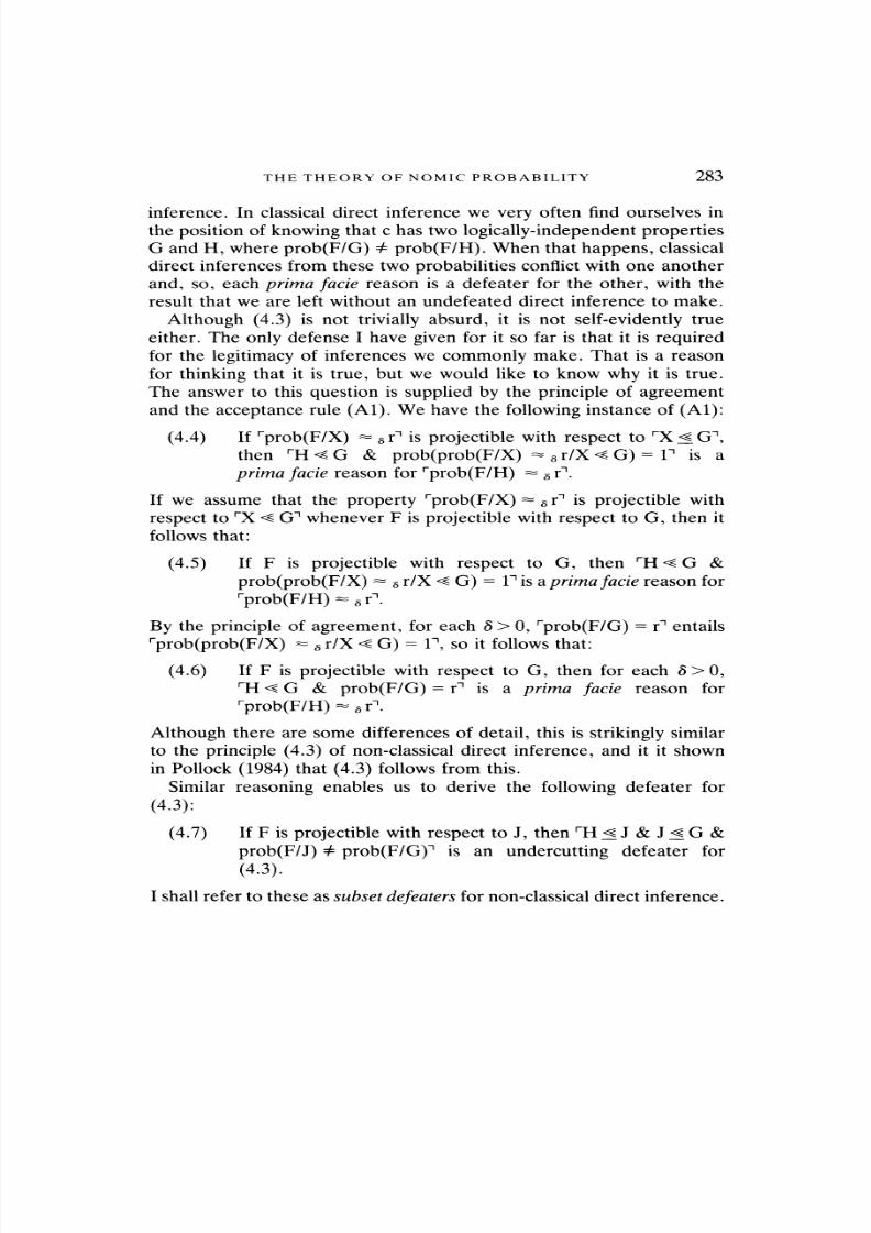
inference. In classical direct inference we very often find ourselves in
the position of knowing that c has two logically-independent propertiesG and H, where prob(F/G) + prob(F/H). When that happens, classical
direct inferences from these two probabilities conflict with one another
and, so, each prima facie reason is a defeater for the other, with the
result that we are left without an undefeated direct inference to make.
Although (4.3) is not trivially absurd, it is not self-evidently true
either. Theonly
defense I havegiven
for it so far is that it isrequired
for the legitimacy of inferences we commonly make. That is a reason
for thinking that it is true, but we would like to know why it is true.
The answer to this question is supplied by the principle of agreement
and the acceptance rule (Al). We have the following instance of (Al):
(4.4) If rprob(F/X)?
?rn is projectible with respect to rX^Gn,
then rH<^G & prob(prob(F/X)?
? r/X < G)= V is a
prima facie reason for rprob(F/H)~
? r~\
If we assume that the property rprob(F/X)?
? r-1 is projectible with
respect to rX < G-1 whenever F is projectible with respect to G, then itfollows that:
(4.5) If F is projectible with respect to G, then rH<^G &
prob(prob(F/X)~
? r/X <^G)
= ln is aprima facie reason for
rprob(F/H)-?rn.
By the principle of agreement, for each 8 > 0, rprob(F/G)= r"1 ntails
rprob(prob(F/X)?
Sr/X < G)=
V, so it follows that:
(4.6) If F is projectible with respect to G, then for each 8>0,
rH < G &prob(F/G)
= r"1is
aprima facie
reasonfor
rprob(F/H)-?rn.
Although there are some differences of detail, this is strikingly similar
to the principle (4.3) of non-classical direct inference, and it it shown
in Pollock (1984) that (4.3) follows from this.
Similar reasoning enables us to derive the following defeater for
(4.3):
(4.7) If F is projectible with respect to J, then rH^J&J^G&
prob(F/J) + prob(F/G)n is an undercutting defeater for
(4.3).
I shall refer to these as subset defeaters for non-classical direct inference.
8/8/2019 Nomic Probability
http://slidepdf.com/reader/full/nomic-probability 23/38
284 JOHN L. POLLOCK
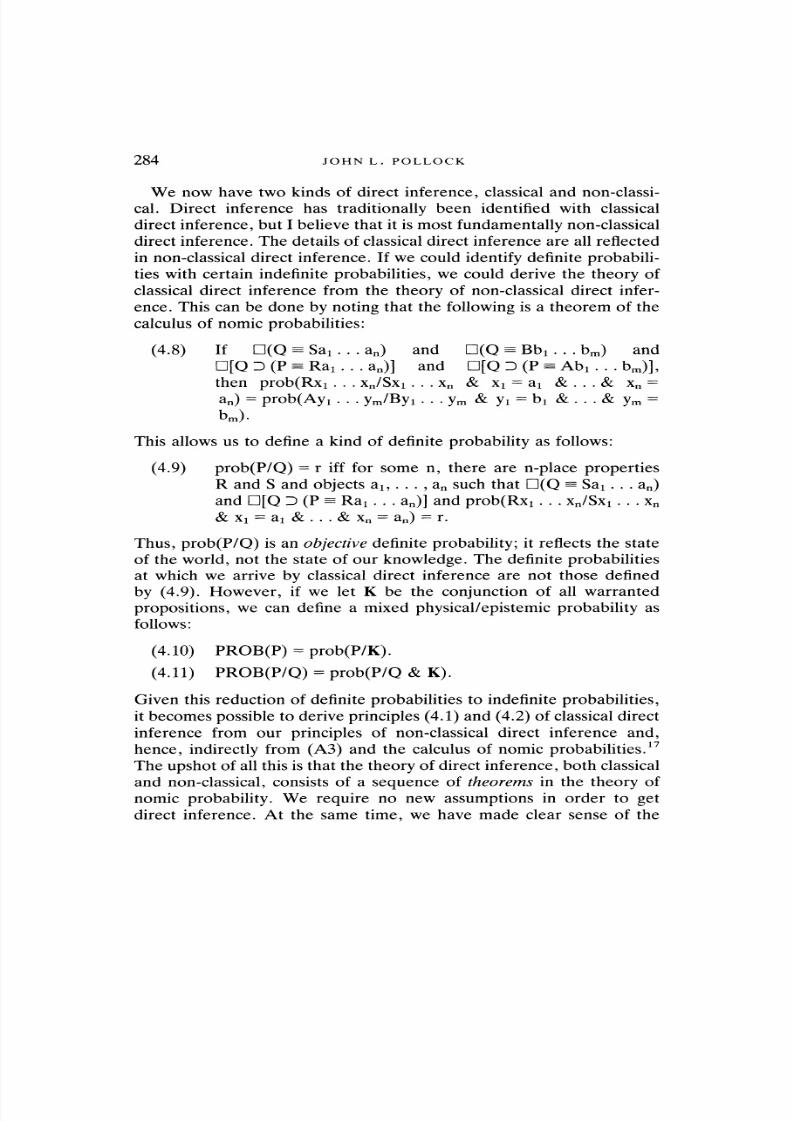
We now have two kinds of direct inference, classical and non-classi
cal. Direct inference has traditionally been identified with classical
direct inference, but I believe that it ismost fundamentally non-classical
direct inference. The details of classical direct inference are all reflected
in non-classical direct inference. If we could identify definite probabili
ties with certain indefinite probabilities,we could derive the theory of
classical direct inference from the theory of non-classical direct infer
ence. This can be doneby noting
that thefollowing
is a theorem of the
calculus of nomic probabilities:
(4.8) If D(Q=
Sai. . .an) and D(Q
^Bbx . . .
bm) and
D[Q D (Ps
Rai. . .an)] and D[Q D (P
=Abi . . .
bm)],
thenprob(Rxi
. . .xn/Sxi
. . .xn & xx
=ax & ... & xn
=
a?)=
prob(Ayi.. .
ym/Byi.. .
ym & y1=
bi & . . .& ym=
bm).
This allows us to define a kind of definite probabilityas follows:
(4.9) prob(P/Q)
=
r iff for some n, there are n-place propertiesR and S and objects ai? . . . ,an such that D(Q
=Sai. . .
an)
and D[Q D (P=
Rax. . .an)] and prob(Rxx
. . .xn/Sxi . . .xn
& Xi=
ai & . . .& xn=
an)= r.
Thus, prob(P/Q) is an objective definite probability; it reflects the state
of the world, not the state of our knowledge. The definite probabilitiesat which we arrive by classical direct inference are not those defined
by (4.9). However, if we let K be the conjunction of all warranted
propositions,we can define a mixed physical/epistemic probability as
follows:
(4.10) PROB(P)=
prob(P/K).
(4.11) PROB(P/Q)=
prob(P/Q & K).
Given this reduction of definite probabilities to indefinite probabilities,
it becomes possible to derive principles (4.1) and (4.2) of classical direct
inference from our principles of non-classical direct inference and,
hence, indirectly from (A3) and the calculus of nomic probabilities.17The upshot of all this is that the theory of direct inference, both classical
and non-classical, consists of a
sequence
of theorems in the
theory
of
nomic probability. We require no new assumptions in order to get
direct inference. At the same time, we have made clear sense of the
8/8/2019 Nomic Probability
http://slidepdf.com/reader/full/nomic-probability 24/38
THE THEORY OF NOMIC PROBABILITY 285
mixed physical/epistemic probabilities that are needed for decision the
ory.
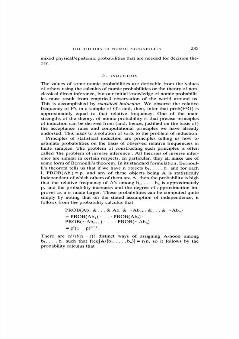
5. INDUCTION
The values of some nomic probabilitiesare derivable from the values
of others using the calculus of nomic probabilities or the theory of non
classical direct inference, but our initial knowledge of nomic probabilities must result from empirical observation of the world around us.
This is accomplished by statistical induction. We observe the relative
frequency of F's in a sample of G's and, then, infer that prob(F/G) is
approximately equal to that relative frequency. One of the main
strengths of the theory, of nomic probability is that precise principlesof induction can be derived from (and, hence, justified on the basis of)
the acceptance rules and computational principles we have already
endorsed. This leads to a solution of sorts to the problem of induction.
Principles of statistical induction are principles telling us how to
estimate probabilities on the basis of observed relative frequencies in
finite samples. The problem of constructing such principles is often
called 'the problem of inverse inference'. All theories of inverse infer
ence are similar in certain respects. In particular, they all make use of
some form of Bernoulli's theorem. In its standard formulation, Bernoul
li's theorem tells us that if we have n objects bi, . . . ,bn and for each
i, PROB(Abi)=
p, and any of these objects being A is statistically
independent of which others of them are A, then the probability is highthat the relative frequency of A's among b1? . . . ,bn is approximately
p, and the probability increases and the degree of approximation im
proves as n is made larger. These probabilitiescan be computed quite
simply by noting that on the stated assumption of independence, it
follows from the probability calculus that
PROB(Abx & . . .& Abr & ~Abr+1 & ... & ~Abn)
=PROB(Abx)
. . .PROB(Abr)
PROB(~Abr+1). . .
PROB(~Abn)
-pr(i-prr.
There are n!/r!(n-r)! distinct ways of
assigning
A-hood among
bi,. . ., bn such that freq[A/{bi,. . . ,bn}]
=r/n, so it follows by the
probability calculus that
8/8/2019 Nomic Probability
http://slidepdf.com/reader/full/nomic-probability 25/38
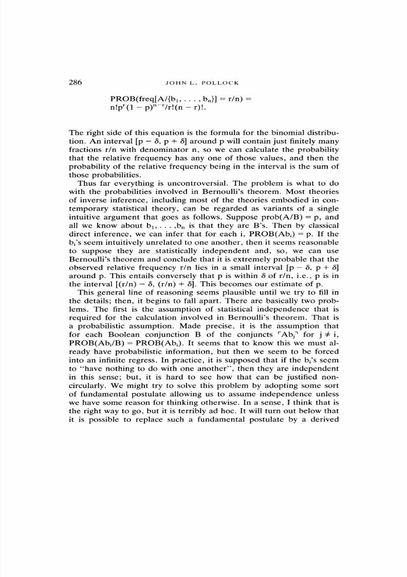
286 JOHN L. POLLOCK
PROB(freq[A/{bi,. . . ,bn}]
=r/n)
=
n!pr(l-p)n-7r!(n-r)!.
The right side of this equation is the formula for the binomial distribu
tion. An interval [p-
8, p +8] around p will contain just finitely many
fractions r/n with denominator n, so we can calculate the probability
that the relativefrequency
hasany
one of thosevalues,
and then the
probability of the relative frequency being in the interval is the sum of
those probabilities.
Thus far everything is uncontroversial. The problem is what to do
with the probabilities involved in Bernoulli's theorem. Most theories
of inverse inference, including most of the theories embodied in con
temporary statistical theory, can be regarded as variants of a single
intuitive argument that goes as follows. Suppose prob(A/B)=
p, and
all we know about bi,. . . ,bn is that they are B's. Then by classical
direct inference, we can infer that for each i, PROB (Abi)=
p. If the
bi's seem intuitively unrelated to one another, then it seems reasonableto suppose they are statistically independent and, so, we can use
Bernoulli's theorem and conclude that it is extremely probable that the
observed relative frequency r/n lies in a small interval [p-
8, p +8]
around p. This entails conversely that p is within 8 of r/n, i.e., p is in
the interval [(r/n)-
8, (r/n)+
8]. This becomes our estimate of p.
This general line of reasoning seems plausible until we try to fill in
the details; then, it begins to fall apart. There are basically two problems. The first is the assumption of statistical independence that is
required for the calculation involved in Bernoulli's theorem. That is
a probabilistic assumption. Made precise, it is the assumption that
for each Boolean conjunction B of the conjuncts '"Abj-1 for j + i,
PROB(Abi/B)=
PROB(Abi). It seems that to know this we must al
ready have probabilistic information, but then we seem to be forced
into an infinite regress. In practice, it is supposed that if the bi's seem
to "have nothing to do with one another", then they are independent
in this sense; but, it is hard to see how that can be justified non
circularly. We might try to solve this problem by adopting some sort
of fundamental postulate allowing us to assume independence unless
we have some reason forthinking
otherwise. In a sense, I think that is
the right way to go, but it is terribly ad hoc. It will turn out below that
it is possible to replace such a fundamental postulate by a derived
8/8/2019 Nomic Probability
http://slidepdf.com/reader/full/nomic-probability 26/38
THE THEORY OF NOMIC PROBABILITY 287
principle following from the parts of the theory of nomic probability
that have already been established.
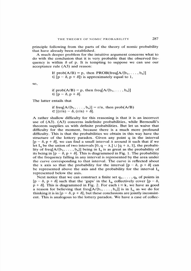
A much deeper problem for the intuitive argument concerns what to
do with the conclusion that it is very probable that the observed fre
quency is within ? of p. It is tempting to suppose we can use our
acceptance rule (A3) and reason:
If prob(A/B)=
p, then PROB(freq[A/{b!,.. . ,bn}]
E [p- 8, p + 8]) is approximately equal to 1,
so,
if prob(A/B)=
p, then freq[A/{b1?. . . ,bn}]
e[p-S,p+
S].
The latter entails that
if freq[A/{bi,. . . ,bn}]
=r/n, then prob(A/B)
E [(r/n)-5, (r/n)+ 5].
A rather shallow difficulty for this reasoning is that it is an incorrect
use of (A3). (A3) concerns indefinite probabilities, while Bernoulli's
theorem suppliesus with definite probabilities. But let us waive that
difficulty for the moment, because there is a much more profound
difficulty. This is that the probabilitieswe obtain in this way have the
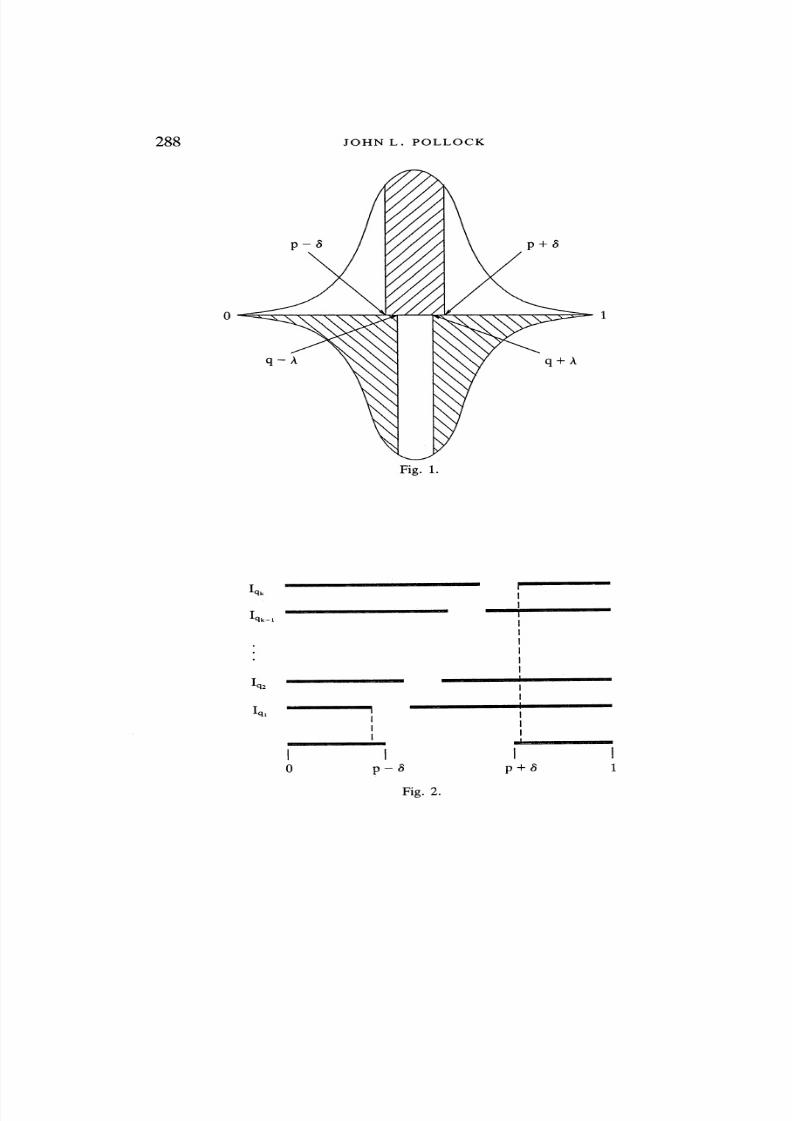
structure of the lottery paradox. Given any point q in the interval
[p-
8, p +8], we can find a small interval ? around it such that if we
let Iq be the union of two intervals [0, q-
A,] U [q+ A, 1], the probabi
lity of freq[A/{bi,. . . ,bn}] being in
Iqis as great as the probability of
its being in [p - 8, p + 8]. This is diagrammed in Fig. 1. The probability
of the frequency falling in any interval is represented by the area under
the curve corresponding to that interval. The curve is reflected about
the x axis so that the probability for the interval [p-
8, p 4-8] can
be represented above the axis and the probability for the interval Iq
represented below the axis.
Next notice that we can construct a finite set q1?.. . ,qk of points in
[p-
8, p +8] such that the 'gaps' in the Iqi collectively cover [p
-8,
p +5]. This is diagrammed in Fig. 2. For each i< k, we have as good
a reason forbelieving
thatfreq[A/{bi,
. . . ,bn}]
is inIqi
as we do for
thinking it is in [p-
8, p + 8], but these conclusions are jointly inconsist
ent. This is analogous to the lottery paradox. We have a case of collec
8/8/2019 Nomic Probability
http://slidepdf.com/reader/full/nomic-probability 27/38
288 JOHN L. POLLOCK
Fig. 1.
p-a
Fig. 2.
p + 5
8/8/2019 Nomic Probability
http://slidepdf.com/reader/full/nomic-probability 28/38
THE THEORY OF NOMIC PROBABILITY 289
tive defeat and, thus, are unjustified in concluding that the relative
frequency is in the interval [p-
8, p + 8].
The intuitive response to the 'lottery objection' consists of notingthat [p
-8, p +
8] is an interval while the Iqare not. Somehow, it seems
right to make an inference regarding intervals when it is not right to
make the analogous inference regarding 'gappy' sets. That is the line
taken in orthodox statistical inference when confidence intervals are
employed. But,it is
veryhard to see
whythis should be the
case,and some heavy-duty argument is needed here to justify the whole
procedure.
In sum, when we try to make the intuitive argument precise, it
becomes apparent that it contains major lacunae. This does not consti
tute an utter condemnation of the intuitive argument. Because it is so
intuitive, it would be surprising if it were not at least approximately
right. Existing statistical theories tend to be ad hoc jury-rigged affairs
without adequate foundations, but it seems there must be some sound
intuitions that statisticians are trying to capture with these theories.18
The problem is to turn the intuitive argument into a rigorous anddefensible argument. That, in effect, is what my account of statistical
induction does. The argument will undergo three kinds of repairs,
creating what I call the statistical induction argument. First, it will be
reformulated in terms of indefinite probabilities, thus enabling us to
make legitimate use of our acceptance rules. Second, it will be shown
that the gap concerning statistical independence can be filled by non
classical direct inference. Third, the final step of the argument will be
scrapped and replaced by a morecomplex argument not subject to the
lottery paradox. This morecomplex argument will employ
aprinciple
akin to the Likelihood Principle of classical statistical inference.
The details of the statistical induction argument are complicated, and
can be found in full in Pollock (1984a and 1990). I will try to convey
the gist of the argument by focusing on a special case. Normally,
prob(A/B)can have any value from 0 to 1. The argument is complicated
by the fact that there are infinitely many possible values. Let us suppose
instead that we somehow know that prob(A/B) has one of a finite set
of values pi,.. . ,pk. If we have observed a
sample X ={bi,
. . . ,bn}
of B's and noted that only b1?. . . ,br are A's (where A and ~A are
projectible with respect to B), then the relative
frequency freq[A/X]of A's in X is r/n. From this we want to infer that prob(A/B) is
approximately r/n. Our reasoning proceeds in two stages, the first stage
8/8/2019 Nomic Probability
http://slidepdf.com/reader/full/nomic-probability 29/38
290 JOHN L. POLLOCK
employing the theory of non-classical direct inference, and the second
stage employing our acceptance rules.
Stage I
Let us abbreviate rXi,...,xn are distinct & Bx &. . .& Bx &
prob(Ax/Bx)=
p"1asr0pn.When r^ n, n, we have by the probability
calculus:
(5.1) prob(Axx & . . .& Ax4 & ~Axr+1 & ... & ~Axn/0p)
=prob(Axx/Ax2 & ..& Axr & ~Axr+1 & ... & ~Axn &
0P)
. . .prob(Axr/~Axr+i
& ... & ~Axn &0P)
prob(~Axr+i/~Axr+2 & ... & ~Axn &0P)
. . .prob(~Axn/0p).
Making 0P explicit:
(5.2) prob(AXi/Axi+1
& . . .& Axr & ~Axr+1 & ... & ~Axn &
0P)=
prob(Ax?/xi,. . . , xn are distinct
& Bxx & . . .& Bxn & Axn+1 & . . .& Axr
& ?Axr+1 & ... & ~Axn & prob(A/B)
=p).
Projectibility is closed under conjunction, so rAxin is projectible with
respect to rBxx & ... & Bxn & xl5 . . . ,xn are distinct & Axi+1 & . . .&
Axr & ~Axr+i & ... & ~Axnn. Given principles we have already en
dorsed, it can be proven that whenever ""Axi-1s projectible with respect
toTFx"1,
it is alsoprojectible
withrespect
to rFx &prob(Ax/Bx)
=
p"1.Consequently, ""Axf is projectible with respect to the reference property
of (5.2). Thus a non-classical direct inference gives us a reason for
believing that:
prob(AXi/Axi+1 & . . .& Axr & ~Axr+1 & ... & ~Axn &0P)
=prob(Axi/BXi & prob(A/B)
=p),
which by principle (PPROB) equals p. Similarly, non-classical direct
inference gives us a reason for believing that if r< i^ n then,
(5.3) prob(~AXi/~Axi+1 & ... & ~Axn & 0P) = 1-
p.
Then from (5.1) we have:
8/8/2019 Nomic Probability
http://slidepdf.com/reader/full/nomic-probability 30/38
THE THEORY OF NOMIC PROBABILITY 291
(5.4) prob(AXi & . . .& Axr & ~Axr+1 & ... &~Axn/0p)
=pr(i-prr.
rfreq[A/{xi,. . . ,xn}]
= r/n"1 is equivalent to a disjunction of
n!/r!(n-
r)! pairwise incompatible disjuncts of the form rAxi & ... &
Axr & ~Axr+1 & ... & ~Axnn, so, by the probability calculus:
(5.5) prob(freq[A/{Xl,. . .
,xn}] =r/n/0p)=n!pr(l-p)n"r/r!(n-r)!.
This is the formula for the binomial distribution.
This completes Stage I of the statistical induction argument. This
stage reconstructs the first half of the intuitive argument described in
Section 1. Note that it differs from that argument in that it proceedsin terms of indefinite probabilities rather than definite probabilities,and it avoids having to make unwarranted assumptions about independence by using non-classical direct inference instead. In effect, non
classical direct inferencegives
us a reasonfor expecting independence,
unless we have evidence to the contrary. All of this is a consequence
of our acceptance rule and computational principles.
Stage II
The second half of the intuitive argument ran afoul in the lottery
paradox and seems to me to be irreparable. I propose to replace it with
an argument using (A2). I assume at this point that ifA is a projectible
property, then rfreq[A/X] ?^ r/n"1 is aprojectible property of X. Thus,
the following conditional probability, derived from (5.5), satisfies the
projectibility constraint of our acceptance rules:
(5.6) prob(freq[A/{xi,. . . ,xn}] ^ r/n / 0P)
=l-n!pr(l-p)n~7r!(n-r)!.
Let b(n, r, p)=
n!pr(l-
p)n~7r!(n-
r)!. For sizable n, b(n, r, p) is al
most always quite small, e.g., b(50, 20, 0.5)= 0.04. Thus, by (A2) and
(5.6), for each choice of p we have a prima facie reason for believingthat (bi,.
. . ,bn) does not satisfy 0P, i.e., for believing
~(bi,.. . ,bn are distinct & Bbi & . . .& Bbn &
prob(A/B)=
p).
8/8/2019 Nomic Probability
http://slidepdf.com/reader/full/nomic-probability 31/38
292 JOHN L. POLLOCK
Because we know that rbi,. . . , bn are distinct & Bbi & ... & Bbnn
is true, this gives us aprima facie reason for believing that
prob(A/B) # p. But, we know that for some one of pi, ...,pk,
prob(A/B)=
pi. This case is much like the case of the lottery para
dox. For each i we have aprima facie reason for believing that
prob(A/B) # pi, but we also have a counterargument for the conclusion
that prob(A/B)=
pi? viz.:
prob(A/B) 7 p!
prob(A/B) # p2
prob(A/B)#pi_!
prob(A/B) 7^pi+1
prob(A/B) t? pk
For some j between 1 and k, prob(A/B)=
pj.
Therefore, prob(A/B)=
pi.
But there is animportant difference between this case and a fair lottery.
For each i, we have a prima facie reason for believing that
prob(A/B) ?" pi5 but these reasons are not all of the same strength
because the probabilities assigned by (5.6) differ for the different pi's.The counterargument is only as good as its weakest link, so for some
of the pi's, the counterargument may not be strong enough to defeat
the prima facie reason for believing that prob(A/B) ^ pA. This will
result in there being a subset R (the rejection class) of {pi,... ,pk} such
that we can conclude that that for each p E R, prob(A/B) ?^ p and,
hence, prob(A/B) ? R. Let A (the acceptance class) be
{pi, ,pk}-
R. It follows that we are justified in believing that
prob(A/B) E A. A will consist of those pi's closest in value to r/n.
Thus, we can think of A as an interval around the observed frequency,
and we are justified in believing that prob(A/B) lies in that interval.
To fill in some details, let us abbreviate 'r/n' as 'f, and make the
simplifying assumption that for some i, pi= f. Then, b(n, r, p) will
always be highest for this value of p, which means that (5.6) providesus with a weaker reason for
believing
that
prob(A/B)
# f than it does
for believing that prob(A/B) ^ pj for any of the other pj's. It follows
that f cannot be in the rejection class, because each step of the coun
8/8/2019 Nomic Probability
http://slidepdf.com/reader/full/nomic-probability 32/38
THE THEORY OF NOMIC PROBABILITY 293
terargument is better than the reason for believing that prob(A/B) t* f.
On the other hand, rprob(A/B) # F will be the weakest step of the
counterargument for every other pj. Thus, what determines whether pj
is in the rejection class is simply the comparison of b(n, r, pj)to
b(n, r, n/r). A convenient way to encode this comparison is by consider
ing the ratio
(5.7) L(n, r, p)=
b(n, r, p)/b(n, r, f )=
(p/f)nf-((l-p)/l-f)n(1-f).
L(n, r, p) is the likelihood ratio of rprob(A/B)= fn to rprob(A/B)
= f1.
The smaller the likelihood ratio, the stronger is our on-balance reason
for believing (despite the counterargument) that prob(A/B) # p and,
hence, the more justified we are in believing that prob(A/B) t? p. Each
degree of justification corresponds to a minimal likelihood ratio, so we
can take the likelihood ratio to be a measure of the degree of justifi
cation. For each likelihood ratio a we obtain the a-rejection class Ra
and the a-acceptance class Aa:
(5.8) Ra=
{Pi |L(n, r, Pi)*=
a}
(5.9) Aa-{pi|L(n,r,Pi)>a}.
We are justified to degreea in rejecting the members of Ra and, hence,
we are justified to degreea in believing that prob(A/B) is a member
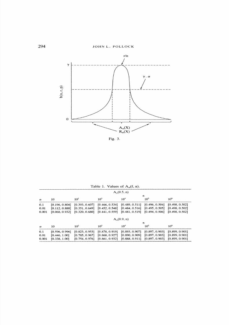
of Aa. If we plot the likelihood ratios, we get a bell curve centered
around r/n, with the result that Aa is an interval around r/n and Ra
consists of the tails of the bell curve. This is shown in Fig. 3. In
interpreting this curve, remember that low likelihood ratios correspond
to a high degree of justification for rejecting that value for prob(A/B)
and, so, the region around r/n consists of those values we cannot reject,
i.e., it consists of those values that might be the actual value.
I have been discussing the idealized case in which we know that
prob(A/B) has one of a finite set of values, but the argument can be
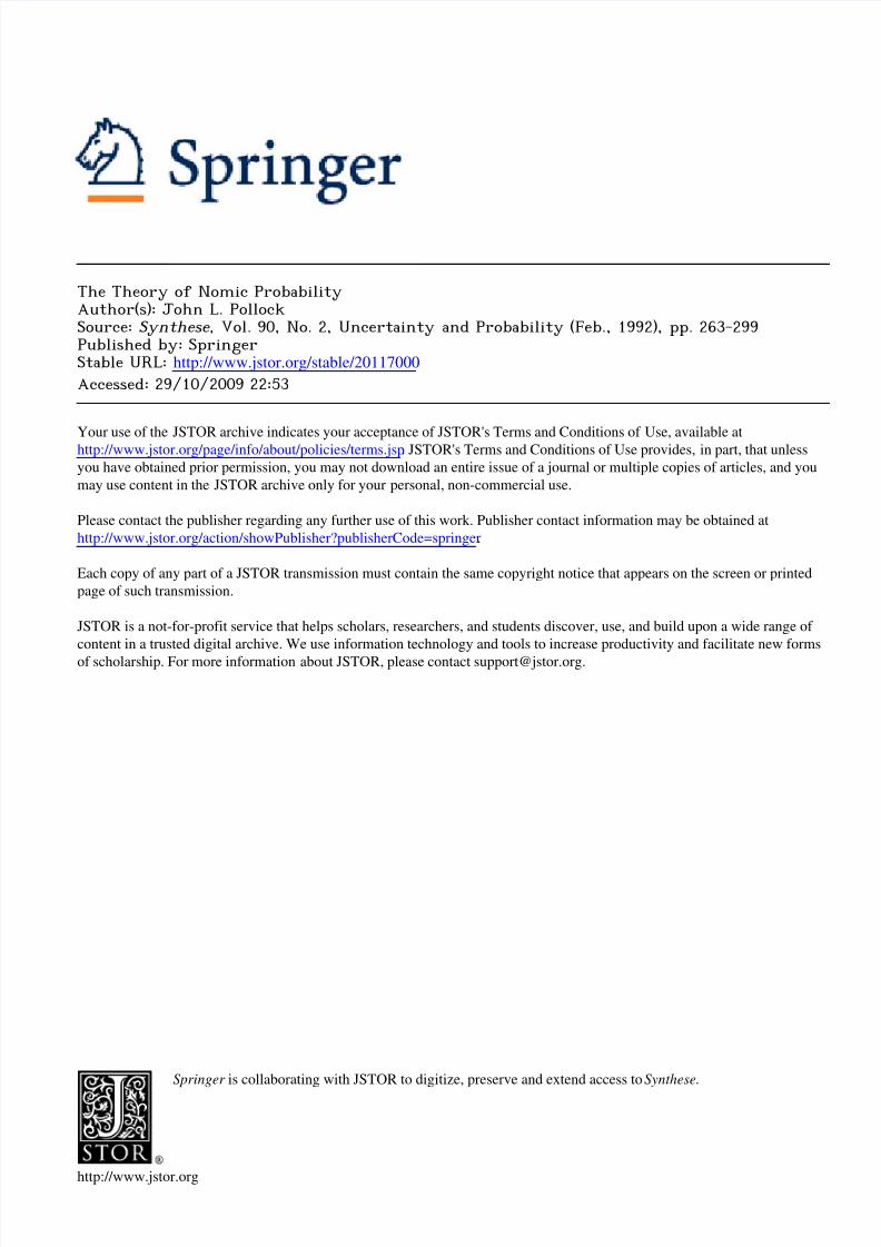
generalized to apply to the continuous case as well. The argument
provides us with justification for believing that prob(A/B) lies in a
precisely-defined interval around the observed relative frequency, the
width of the interval beinga function of the degree of justification. For
illustration, some
typical
values of the
acceptance
interval are listed in
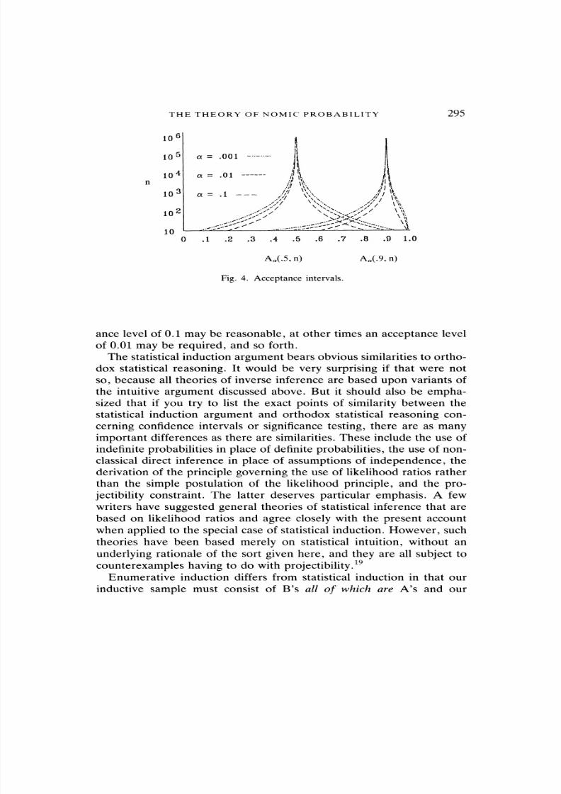
Table 1 and plotted in Fig 4. Reference to the acceptance level reflects
the fact that attributions of warrant are indexical. Sometimes an accept
8/8/2019 Nomic Probability
http://slidepdf.com/reader/full/nomic-probability 33/38
JOHN L. POLLOCK
c
Aa(X)
Ra(X)
Fig. 3.
Table 1. Values of A?(f,n).
10 102 10j
Aa(0.5, n)
104 105 106
0.1 [0.196,0.804]
0.01 [0.112,0.888]
0.001 [0.068,0.932]
10
[0.393,0.607]
[0.351,0.649]
[0.320,0.680]
102
[0.466, 0.534]
[0.452, 0.548]
[0.441,0.559]
[0.489,0.511]
[0.484, 0.516]
[0.481,0.519]
[0.496,0.504] [0.498, 0.502]
[0.495,0.505] [0.498, 0.502]
[0.494, 0.506] [0.498,0.502]
10J
Aa(0.9, n)
104 105 106
0.1 [0.596,0.996]0.01 [0.446,1.00]0.001 [0.338,1.00]
[0.823,0.953] [0.878,0.919] [0.893,0.907] [0.897,0.903] [0.899,0.901]
[0.785,0.967] [0.868,0.927] [0.890,0.909] [0.897,0.903] [0.899,0.901]
[0.754,0.976] [0.861,0.932] [0.888,0.911] [0.897,0.903] [0.899,0.901]
8/8/2019 Nomic Probability
http://slidepdf.com/reader/full/nomic-probability 34/38
THE THEORY OF NOMIC PROBABILITY 295
10?
10'
10'
10'
10'
10
a - .001-
a = .01?
a = .1"I VV>
..^i^^,-. \
.1 .2 .3 .4 .5 .6 .7 .8 .9 1.0
Aa(.5,n) Aa(.9,n)
Fig. 4. Acceptance intervals.
ance level of 0.1 may be reasonable, at other times an acceptance levelof 0.01 may be required, and so forth.
The statistical induction argument bears obvious similarities to ortho
dox statistical reasoning. It would be very surprising if that were not
so, because all theories of inverse inference are based upon variants of
the intuitive argument discussed above. But it should also be emphasized that if you try to list the exact points of similarity between the
statistical induction argument and orthodox statistical reasoning con
cerning confidence intervals or significance testing, there are as many
important differences as there are similarities. These include the use of
indefinite probabilities in place of definite probabilities, the use of non
classical direct inference in place of assumptions of independence, the
derivation of the principle governing the use of likelihood ratios rather
than the simple postulation of the likelihood principle, and the pro
jectibility constraint. The latter deserves particular emphasis. A few
writers have suggested general theories of statistical inference that are
based on likelihood ratios and agree closely with the present account
when applied to the special case of statistical induction. However, such
theories have been based merely on statistical intuition, without an
underlying
rationale of the sort
givenhere, and
they
are all
subject
to
counterexamples having to do with projectibility.19Enumerative induction differs from statistical induction in that our
inductive sample must consist of B's all of which are A's and our
8/8/2019 Nomic Probability
http://slidepdf.com/reader/full/nomic-probability 35/38
296 JOHN L. POLLOCK
conclusion is the generalization rB =>A"1. It is shown in Pollock (1984a
and 1990) that in the special case in which the observed relative fre
quency is 1, our theory of nomic probability allows us to extend the
statistical induction argument to obtain an argument for the conclusion
rB =>A-1. Thus, enumerative induction can also be justified on the basis
of nomic probability.
6. Conclusions
To briefly recapitulate, the theory of nomic probability aims to make
objective probability philosophically respectable by providinga mathe
matically precise theory of probabilistic reasoning. This theory has
two primitive parts: (1) a set of computational principles comprisinga
strengthened probability calculus, and (2) an acceptance rule licensing
defeasible inferences from high probabilities. Some of the compu
tational principles are novel, but the resulting calculus of nomic proba
bilities is still just a strengthened probability calculus. The strengthen
ings are important, but not philosophically revolutionary. The main
weight of the theory is borne by the acceptance rule. But it deserves
to be emphasized that that rule is not revolutionary either. It is just a
tidied-up version of the classical statistical syllogism. What makes the
theory work where earlier theories did not is the explicit appeal to a
theory of defeasible reasoning. It is the importation of state-of-the-art
epistemology that infuses new life into the old ideas on which the theory
of nomic probability is based.
The most remarkable aspect of the theory of nomic probability is
that theories of direct inference and induction fall out as theorems. We
need no new postulates in order to justify these essential kinds of
probabilistic reasoning. In animportant sense, this comprises
a solution
to the problem of induction. Of course, you cannot get something from
nothing, so we are still making epistemological assumptions that Hume
would have found distasteful, but, in animportant sense, principles of
induction have been derived from principles that areepistemologically
more basic.
NOTES
1Pollock 1986, p. 97ff.
2In Pollock 1983, 1983a, 1984, 1984a, 1986a, 1987a.
8/8/2019 Nomic Probability
http://slidepdf.com/reader/full/nomic-probability 36/38
THE THEORY OF NOMIC PROBABILITY 297
3Pollock 1990.
4The concept of a nomic generalization is introduced in Pollock (1974a), and discussed
itmore fully in Pollock (1976). I have previously called nomic generalizations 'subjunctive
generalizations'.5
See Pollock 1987a.6
For this purpose, we must augment (2.1) with aprinciple characterizing counterlegal
nomic probabilities, as in Pollock (1987a).7
Examining the definition of nomic probability in terms of proportions reveals that what
would be required to get the cross product principle for probabilities is not (2.13) but,
rather,
9>({(w,x, y> |Awx & Bwy}/{(w, x, y) |Cwy & Dwy})
=9>({<w,x> |Awx}/{(w, x> |Cwy}) 0>({<w,y) |Bwy}/{(w, y) |Dwy}),
but this principle has nothing to recommend it.8
This stems mainly from the work of Roderick Chisholm and Pollock. See Chisholm
1957, 1977, 1981 and Pollock 1967, 1968, 1971, 1974, 1986. See also Kyburg 1974, 1983.9
For a defense of this, see Pollock (1974, 1986).10
In Pollock 1974.11
In Pollock (1974) rebutting and undercutting defeaters are called 'type F and 'type IF
defeaters, respectively.12
Researchers in artificial intelligence became interested in defeasible reasoning at about
the same time asphilosophers. In AI this led to the current theories of 'nonmonotonic
reasoning'. This is represented by the work of Doyle (1979), Etherington (1983), McCar
thy (1980, 1984),McDermott (1982),McDermott andDoyle (1980), Nute (1986, 1987,
1988), Poole (1985), Reiter (1980), and others. In both philosophy and AI, undercutting
defeaters have generally been overlooked, leading to accounts that do not capture the
full logical structure of defeasible reasoning.13
The lottery paradox is due to Kyburg (1961).14
Kyburg (1970) draws a different conclusion, namely, that we can be justified in holding
inconsistent sets of beliefs, and that it is not automatically reasonable to adopt the
conjunction of beliefs one justifiably holds (i.e., adjunction fails). I am not going to
discuss this position here. Iwill just assume that adjunction is a correct rule of reasoning.
For a discussion of Kyburg's position,see Pollock (1986, pp. 105-12).
15Given certain reasonable assumptions about the operation of prima facie reasons,
(Al), (A2) and (A3) turn out to be equivalent.16
To say that q> is warranted (relative to aparticular epistemic situation) is to say that
an ideal reasoner in that epistemic situation would be justified in believing <p.Warrant
has the important property of being closed under deductive consequence.17
For the details, see Pollock (1984 and 1990).18
In thus chastising existing statistical theory, I take it that I am not saying anything
controversial. It seems to be pretty generally realized that the foundations of statistical
theory are a mess. For discussions of some of this, see Birnbaum (1969), Cox (1958),
Dempster (1964, 1966), Kyburg (1974, p. 51ff.), Pratt (1961), and Seidenfeld (1979).19See particularly Hacking (1965), Gillies (1973), and Edwards (1972). See also Fisher
(1921, 1922) and Barnard (1949, 1966, 1967).
8/8/2019 Nomic Probability
http://slidepdf.com/reader/full/nomic-probability 37/38
298 JOHNL. POLLOCK
REFERENCES
Barnard, G. A.: 1949, 'Statistical Inference', Journal of the Royal Statistical Society BII,
115-49.
Barnard, G. A.: 1966, 'The Use of the Likelihood Function in Statistical Practice',
Proceedings V Berkeley Symposium on Mathematical Statistics and Probability I, 27
40.
Barnard, G. A.: 1967, 'The Bayesian Controversy in Statistical Inference', /. Inst. Actuar.
93, 229-69.
Birnbaum, Allan: 1969, 'Concepts of Statistical Inference', in S. Morganbesser, P.
Suppes, and M. White (eds.), Philosophy, Science, and Method, St. Martin's Press,
New York, pp. 112-43.
Chisholm, Roderick: 1957, Perceiving, Cornell University Press, Ithaca.
Chisholm, Roderick: 1977, Theory of Knowledge. 2d. edn., Prentice Hall, Englewood
Cliffs NJ.
Chisholm, Roderick: 1981, 'A Version of Foundationalism', Midwest Studies in Philoso
phy, eds. P. A. French, T. E. Uehling, and H. K. Wettstein, University of Minnesota
Press, Minneapolis, Vol. V, pp. 543-64.
Cox, D. R.: 1958, 'Some Problems Connected With Statistical Inference', Annals of
Mathematical Statistics 29, 357-63.
Dempster, A. P.: 1964, 'On the Difficulties Inherent in Fisher's Fiducial Argument',
Journal of the American Statistical Association 59, 56-66.
Dempster, A. P.: 1966, 'Review of The Logic of Statistical Inference', Journal of the
American Statistical Association 61, 1233-35.
Doyle, J.: 1979, 'A Truth Maintenance System', Artificial Intelligence 12, 231-72.
Edwards, A. W. F.: 1972, Likelihood, Cambridge University Press, Cambridge.
Etherington, D. W.: 1983, Formalizing Nonmonotonic Reasoning Systems, Computer
Science Tech. Report No. 83-1, University of British Columbia, Vancouver BC.
Fisher, R. A.: 1921, 'On the 'Probable Error' of a Coefficient of Correlation Deduced
From a Small Sample', Metron I(Pt. 4), 3-32.
Fisher, R. A.: 1922, 'On the Mathematical Foundations of Theoretical Statistics', Philo
sophical Transactions of the Royal Society 222 (Series A), 309-68.
Gillies,D. A.:
1973,An
Objective Theory of Probability,Methuen, London.
Goodman, Nelson: 1955, Fact, Fiction, and Forecast, Harvard University Press, Cam
bridge MA.
Hacking, Ian: 1965, Logic of Statistical Inference, Cambridge University Press, Cam
bridge.
Kolmogoroff, A. N.: 1933, Grundbegriffe der Wahrscheinlichkeitsrechnung, Julius
Springer, Berlin.
Kyburg, Henry, Jr.: 1961, Probability and the Logic of Rational Belief, Wesleyan Univer
sity Press, Middletown CT.
Kyburg, Henry, Jr.: 1970, 'Conjunctivitis', in Marshall Swain (ed.), Induction, Accept
ance, and Rational Belief, D. Reidel, Dordrecht, pp. 55-82.
Kyburg, Henry, Jr.: 1974, The Logical Foundations of Statistical Inference, D. Reidel,
Dordrecht.
Kyburg, Henry, Jr.: 1983, 'The Reference Class', Philosophy of Science 50, 374-97.
McCarthy, J.: 1980, 'Circumscription- a Form of Nonmonotomic Reasoning', Artificial
Intelligence 13, 27-39.
8/8/2019 Nomic Probability
http://slidepdf.com/reader/full/nomic-probability 38/38
THE THEORY OF NOMIC PROBABILITY 299
McCarthy, J.: 1984, 'Applications of Circumscription to Formalizing Common Sense
Knowledge', Proceedings of the Nonmonotonic Reasoning Workshop, New Platz NY,
pp. 295-324.
McDermott, D. V.: 1982, 'Nonmonotonic Logic II: Monmonotonic Modal Theories', /.
ACM 29(1), 33-57.
McDermott, D. V. and J. Doyle: 1980, 'Nonmonotonic Logic F, Artificial Intellience 13,
41-72.
Nute, D.: 1986, LDR: A Logic for Defeasible Reasoning, ACMA Research Report No.
01-0013, University of Georgia, Athens GA.
Nute, D.: 1987, 'Defeasible Reasoning', Proceedings of the Twentieth Annual Hawaii
International Conference on Systems Sciences, University of Hawaii, Honolulu, pp.
470-77.
Nute, D.: 1988, 'Defeasible Reasoning: aPhilosophical Analysis in Prolog', in J. Fetzer
(ed.), Aspects of AI, D. Reidel, Dordrecht, pp. 251-88.
Pollock, John: 1967, 'Criteria and Our Knowledge of the Material World', The Philosoph
ical Review LXXVI, 28-60.
Pollock, John: 1968, 'What is anEpistemological Problem', American Philosophical
Quarter 5, 183-90.
Pollock, John: 1971, 'Perceptual Knowledge', Philosophical Review LXXX, 287-319.
Pollock, John: 1974, Knowledge and Justification, Princeton University Press, Princeton.
Pollock, John: 1974a, 'Subjunctive Generalizations', Synthese 28, 199-214.
Pollock, John: 1976, Subjunctive Reasoning, D. Reidel, Dordrecht.
Pollock, John: 1983, 'A Theory of Direct Inference', Theory and Decision 15, 29-96.
Pollock, John: 1983a, 'Epistemology and Probability', Synthese 55, 231-52.
Pollock, John: 1984, 'Foundations for Direct Inference', Theory and Decision 17, 221
56.
Pollock, John: 1984a, 'A Solution to the Problem of Induction', Nous 18, 423-61.
Pollock, John: 1986, Contemporary Theories of Knowledge, Rowman and Littlefield,
Totowa NJ.
Pollock, John: 1986a, 'The Paradox of the Preface', Philosophy of Science 53, 246-58.
Pollock, John: 1987, 'Defeasible Reasoning', Cognitive Science 11, 481-518.
Pollock, John: 1987a, 'Probability and Proportions', inH. Berghel and G. Eberlein (eds.),
Theoryand Decision:
EssaysinHonor
ofWerner
Leinfellner,D.
Reidel,Amsterdam.
Pollock, John: 1990, Nomic Probability and the Foundations of Induction, Oxford Univer
sity Press, New York.
Poole, D.: 1985, 'On the Comparison of Theories: Preferring the Most Specific Explana
tion', Proceedings of the International Joint Conference on AI, Morgan Kaufmann, Los
Angeles.
Pratt, John W.: 1961, 'A Review of E. L. Lehmann's Testing Statistical Hypotheses',
Journal of the American Statistical Association 56, 163-67.
Reiter, R.: 1980, 'A Logic for Default Reasoning', Artificial Intelligence 13, 81-132.
Seidenfeld, Teddy: 1979, Philosophical Problems of Statistical Inference, D. Reidel,
Dordrecht.
Department of Philosophy
University of Arizona
Tucson, AZ 85721
U.S.A.
Recommended