Neural Network Estimator for Electric Field
Distribution on High Voltage Insulators
Abstract-- This paper introduces, a three-dimensional (3D)
neural network electric fields estimator, which will be used to
determine the electric field distribution on high voltage insulator
surface. A 15 KV composite suspension insulator has been used.
In the course of collection the training data sets the finite element
method (FEM) have been used. The collected/used training data
sets consists of x, y and z coordinates of the investigated points
on the insulator surface and operating voltage as NN inputs, and
the electrical fields as NN outputs, i.e. training pairs (input, and
output). Several ANN models have been built, and examined
based on number of NN design considerations, such as number of
layers, number of neurons in each layer, used learning
algorithms, and used performance functions, in order to get the
most efficient trained NN-estimator, which provides the best
generalized approximation ability of NN These developed NNs
make it is possible to determine the electrical fields at any point
on the insulator surface easier and faster. The obtained results
show that the estimated values of electrical field on an acceptable
degree of accuracy. Therefor the ANN models which has been
presented in this paper can be used easily for design and
development processes of the composite insulators for various
line voltages levels.
Keywords: Insulators; Electric Fields; Artificial Neural Networks
(ANN); Back Propagation
I. INTRODUCTION
High voltage insulators is a very important part of the high
voltage electric power transmission systems. Any failure in the
High voltage insulators performance will result in considerable
loss of capital, as there are many industries that depend upon
the continuance of a power supply. The importance of the
research on insulator has been increased with the rise of energy
demand [1].
For high voltage transmission applications, the electric field
and potential distribution calculations, are widely performed in
the design and development operations of the composite
insulators. Control of the electric field within and around high
voltage equipment as conductors, transmission lines, insulators
and associated line hardware, surge arresters, switchgear,
power transformers and rotating machines is a very important
aspect of the design of such equipment. Composite insulators
are being increasingly used by utilities to replace porcelain and
glass insulators because of the advantages obtained from lower
weight, ease of handling, reduced installation and maintenance
cost, increased resistance to vandalism, and superior
contamination performance. Through more than 25 years, of
service experience, the manufacturers and utilities have learned
the importance of controlling the electric field in the vicinity of
the insulators to prevent degradation of the polymeric
insulating materials from corona-related phenomena [2].
In previous study the electric field distribution was
calculated on the surface of the composite insulator using finite
element method (FEM), where a three-dimensional model for
two types of the composite insulators (Alternate Shed and
Straight Shed) were developed, the electric field values on
insulator surface were simulated in two cases: clean/dry, and
contaminated/wet environmental conditions, finally a
comparison of the estimated electric fields on the insulators
surfaces were investigated for the two types [3].
Currently artificial neural networks (ANNs) are being
applied to an increasing number of complex problems due to
their calculation speed, their ability to solve complex non-
linear functions, great efficiency, and robustness and, also in
cases where most of the information for the studied problem is
absent. Many interesting ANN applications have been reported
in power system areas [4].
In this work an alternate sheds insulator will be
investigated, the (FEM) will be used to calculate the induced
electric fields at a huge number of points on the insulator
surface. These calculated electric field values will be used to
train the artificial neural network, and hence the estimated and
calculated electric field values will be compared together, in
order to explore the efficiency of ANN abilities as a universal
approximator. In other words, ANNs were addressed in order
to estimate the electric field across medium voltage composite
insulator, information which is very useful for diagnostic tests
and design procedures.
Actual electric field values and model geometric
coordinates, which were calculated using finite element
method-simulation software on a medium voltage polymeric
(silicon rubber) insulator, are used in order to train, validate
and test the presented ANNs.
Various structures, learning algorithms, and performance
functions for an ANN multi-layer feed-forward back-
propagation network are tested in order to produce the ANN
models with the best generalizing ability. In this paper, and in
the presented ANNs models, the estimation time is very short
to calculate the electric field distribution of HV insulator,
compared with electric field calculations based on the Finite
Element Method.
Mohamed H. Essai, Member IEEE,
Electrical Engineering Department, Al-Azhar University, Qena, Egypt,
Mahmoud. A-H. Ahmed, Electrical Engineering Department,
Al-Azhar University, Qena, Egypt,
Ali. H.I. Mansour, Electrical Engineering Department,
Al-Azhar University, Qena, Egypt,
Refai. A. Refai Electrical Engineering Department,
Al-Azhar University, Cairo, Egypt,
INTERNATIONAL JOURNAL OF SYSTEMS APPLICATIONS, ENGINEERING & DEVELOPMENT Volume 11, 2017
ISSN: 2074-1308 160
II. ELECTRIC FIELD CALCULATION USING FEM
The Finite Element Method (FEM) is a numerical method
of solving Maxwell’s equations in the differential form. The
basic feature of the FEM is to divide the entire problem space,
including the surrounding region, into a number of non-
separated, non-overlapping sub regions, called “finite
elements”. This process is called meshing. These finite
elements can take a number of shapes, but generally triangles
are used for 2-D and 3-D analysis [5].
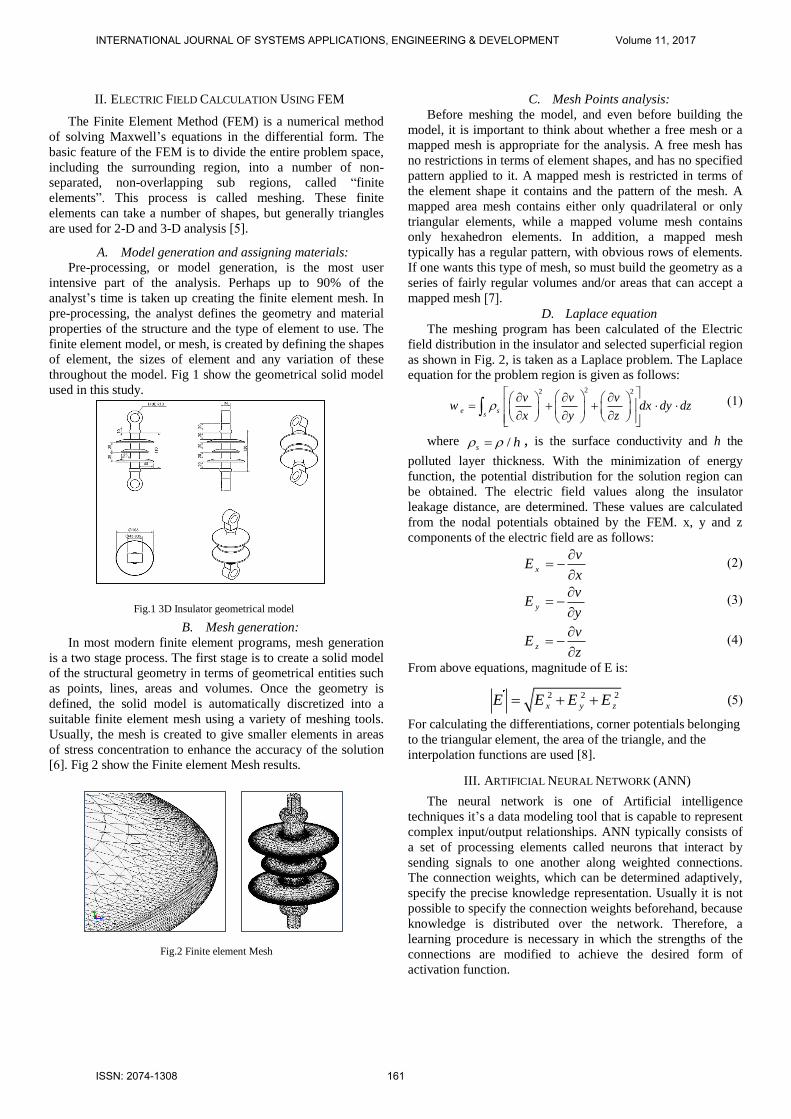
A. Model generation and assigning materials:
Pre-processing, or model generation, is the most user
intensive part of the analysis. Perhaps up to 90% of the
analyst’s time is taken up creating the finite element mesh. In
pre-processing, the analyst defines the geometry and material
properties of the structure and the type of element to use. The
finite element model, or mesh, is created by defining the shapes
of element, the sizes of element and any variation of these
throughout the model. Fig 1 show the geometrical solid model
used in this study.
Fig.1 3D Insulator geometrical model
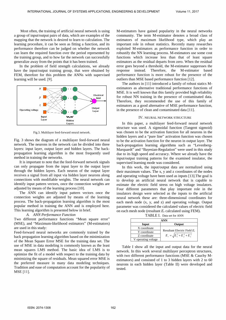
B. Mesh generation:
In most modern finite element programs, mesh generation
is a two stage process. The first stage is to create a solid model
of the structural geometry in terms of geometrical entities such
as points, lines, areas and volumes. Once the geometry is
defined, the solid model is automatically discretized into a
suitable finite element mesh using a variety of meshing tools.
Usually, the mesh is created to give smaller elements in areas
of stress concentration to enhance the accuracy of the solution
[6]. Fig 2 show the Finite element Mesh results.
Fig.2 Finite element Mesh
C. Mesh Points analysis:
Before meshing the model, and even before building the
model, it is important to think about whether a free mesh or a
mapped mesh is appropriate for the analysis. A free mesh has
no restrictions in terms of element shapes, and has no specified
pattern applied to it. A mapped mesh is restricted in terms of
the element shape it contains and the pattern of the mesh. A
mapped area mesh contains either only quadrilateral or only
triangular elements, while a mapped volume mesh contains
only hexahedron elements. In addition, a mapped mesh
typically has a regular pattern, with obvious rows of elements.
If one wants this type of mesh, so must build the geometry as a
series of fairly regular volumes and/or areas that can accept a
mapped mesh [7].
D. Laplace equation
The meshing program has been calculated of the Electric
field distribution in the insulator and selected superficial region
as shown in Fig. 2, is taken as a Laplace problem. The Laplace
equation for the problem region is given as follows: 22 2
e ss
v v vw dx dy dz
x y z
(1)
where /s h , is the surface conductivity and h the
polluted layer thickness. With the minimization of energy
function, the potential distribution for the solution region can
be obtained. The electric field values along the insulator
leakage distance, are determined. These values are calculated
from the nodal potentials obtained by the FEM. x, y and z
components of the electric field are as follows:
x
vE
x
(2)
y
vE
y
(3)
z
vE
z
(4)
From above equations, magnitude of E is:
2 2 2
x y zE E E E (5)
For calculating the differentiations, corner potentials belonging
to the triangular element, the area of the triangle, and the
interpolation functions are used [8].
III. ARTIFICIAL NEURAL NETWORK (ANN)
The neural network is one of Artificial intelligence
techniques it’s a data modeling tool that is capable to represent
complex input/output relationships. ANN typically consists of
a set of processing elements called neurons that interact by
sending signals to one another along weighted connections.
The connection weights, which can be determined adaptively,
specify the precise knowledge representation. Usually it is not
possible to specify the connection weights beforehand, because
knowledge is distributed over the network. Therefore, a
learning procedure is necessary in which the strengths of the
connections are modified to achieve the desired form of
activation function.
INTERNATIONAL JOURNAL OF SYSTEMS APPLICATIONS, ENGINEERING & DEVELOPMENT Volume 11, 2017
ISSN: 2074-1308 161
Most often, the training of artificial neural network is using
a group of input/output pairs of data, which are examples of the
mapping that the network is desired to learn to calculation. The
learning procedure, it can be seen as fitting a function, and its
performance therefore can be judged on whether the network
can learn the required function over the period represented by
the training group, and to how far the network can successfully
generalize away from the points that it has been trained.
In the problem of field strength calculations, we already
have the input/output training group, that were obtained by
FEM, therefore for this problem the ANNs with supervised
learning will be used. [9].
Fig.3. Multilayer feed-forward neural network.
Fig. 3 shows the diagram of a multilayer feed-forward neural
network. The neurons in the network can be divided into three
layers: input layer, output layer and hidden layers. The back-
propagation learning algorithm is the most frequently used
method in training the networks.
It is important to note that the feed-forward network signals
can only propagate from the input layer to the output layer
through the hidden layers. Each neuron of the output layer
receives a signal from all input via hidden layer neurons along
connections with modifiable weights. The neural network can
identify input pattern vectors, once the connection weights are
adjusted by means of the learning process [10].
The ANN can identify input pattern vectors once the
connection weights are adjusted by means of the learning
process. The back-propagation learning algorithm is the most
popular method in training the ANN and is employed here.
This learning algorithm is presented below in brief.
A. ANN Performance Function
Two different performance functions “Mean square error”
(MSE), and “Maximum-likelihood estimators” (M-estimators)
are used in this study:
Feed-forward neural networks are commonly trained by the
back propagation learning algorithm based on the minimization
of the Mean Square Error MSE for the training data set. The
use of MSE in data modeling is commonly known as the least
mean squares LMS method. The basic idea of LMS is to
optimize the fit of a model with respect to the training data by
minimizing the square of residuals. Mean squared error MSE is
the preferred measure in many data modeling techniques.
Tradition and ease of computation account for the popularity of
MSE [11].
M-estimators have gained popularity in the neural networks
community. The term M-estimator denotes a broad class of
estimators of maximum likelihood type, which play an
important role in robust statistics. Recently many researches
exploited M-estimators as performance function in order to
robustify the NN learning process. M-estimators use some cost
functions which increase less than that of least square
estimators as the residual departs from zero. When the residual
error goes beyond a threshold, the M-estimator suppresses the
response instead. Therefore, the M-estimator based
performance function is more robust for the presence of the
outliers than MSE based performance function [12].
The authors in [11] introduced a family of robust statics M-
estimators as alternative traditional performance functions of
MSE. It is well known that this family provided high reliability
for robust NN training in the presence of contaminated data.
Therefore, they recommended the use of this family of
estimators as a good alternative of MSE performance function,
in the presence of clean and contaminated data [11].
IV. NEURAL NETWORK STRUCTURE
In this paper, a multilayer feed-forward neural network
structure was used. A sigmoidal function (Tangent sigmoid)
was chosen to be the activation function for all neurons in the
hidden layers and a “pure line” activation function was chosen
to be the activation function for the neuron in output layer. The
back-propagation learning algorithms such as “Levenberg-
Marquardt” and “Bayesian-Regulation” were used in this study
due to its high speed and accuracy. Where we already have the
input/output training patterns for the examined insulator, the
supervised learning mode was considered.
In this work, the input/output data are normalized using
their maximum values. The x, y and z coordinates of the nodes
and operating voltage have been used as inputs [13].The goal is
to develop an artificial neural network that is capable to
estimate the electric field stress on high voltage insulators.
Four different parameters that play important role in the
insulators design were selected as the inputs to the artificial
neural network these are: three-dimensional coordinates for
each mesh node (x, y, and z) and operating voltage. Output
parameter was considered the calculated values of electric field
on each mesh node (resultant Er calculated using FEM).
TABLE I. Data set for ANN
Table I show all the input and output data for the neural
network. In this work several multilayer perceptron structures,
with two different performance functions (MSE & Cauchy M-
estimators) and consisted of 1 to 3 hidden layers with 2 to 60
neurons in each hidden layer (Table II) were developed and
tested.
ANN Input Output
X coordinate Resultant Electric Field Er
2 2 2
r x y zE E E E Y coordinate
Z coordinate
V operating voltage
INTERNATIONAL JOURNAL OF SYSTEMS APPLICATIONS, ENGINEERING & DEVELOPMENT Volume 11, 2017
ISSN: 2074-1308 162
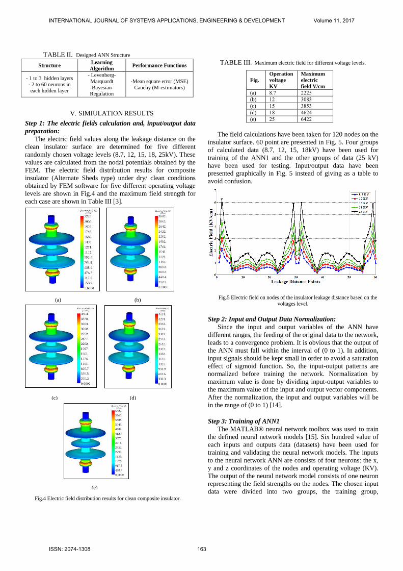
TABLE II. Designed ANN Structure
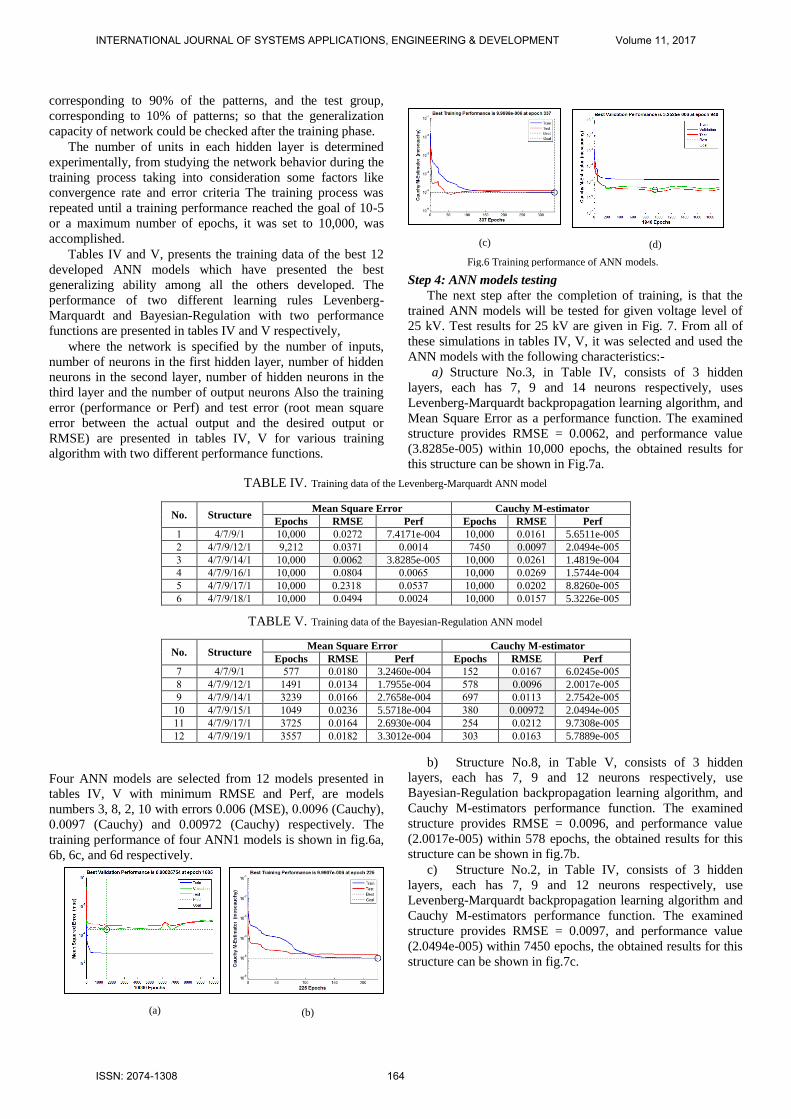
V. SIMIULATION RESULTS
Step 1: The electric fields calculation and, input/output data
preparation:
The electric field values along the leakage distance on the
clean insulator surface are determined for five different
randomly chosen voltage levels (8.7, 12, 15, 18, 25kV). These
values are calculated from the nodal potentials obtained by the
FEM. The electric field distribution results for composite
insulator (Alternate Sheds type) under dry/ clean conditions
obtained by FEM software for five different operating voltage
levels are shown in Fig.4 and the maximum field strength for
each case are shown in Table III [3].
Fig.4 Electric field distribution results for clean composite insulator.
TABLE III. Maximum electric field for different voltage levels.
The field calculations have been taken for 120 nodes on the
insulator surface. 60 point are presented in Fig. 5. Four groups
of calculated data (8.7, 12, 15, 18kV) have been used for
training of the ANN1 and the other groups of data (25 kV)
have been used for testing. Input/output data have been
presented graphically in Fig. 5 instead of giving as a table to
avoid confusion.
Fig.5 Electric field on nodes of the insulator leakage distance based on the
voltages level.
Step 2: Input and Output Data Normalization:
Since the input and output variables of the ANN have
different ranges, the feeding of the original data to the network,
leads to a convergence problem. It is obvious that the output of
the ANN must fall within the interval of (0 to 1). In addition,
input signals should be kept small in order to avoid a saturation
effect of sigmoid function. So, the input-output patterns are
normalized before training the network. Normalization by
maximum value is done by dividing input-output variables to
the maximum value of the input and output vector components.
After the normalization, the input and output variables will be
in the range of (0 to 1) [14].
Step 3: Training of ANN1
The MATLAB® neural network toolbox was used to train
the defined neural network models [15]. Six hundred value of
each inputs and outputs data (datasets) have been used for
training and validating the neural network models. The inputs
to the neural network ANN are consists of four neurons: the x,
y and z coordinates of the nodes and operating voltage (KV).
The output of the neural network model consists of one neuron
representing the field strengths on the nodes. The chosen input
data were divided into two groups, the training group,
Structure Learning
Algorithm Performance Functions
- 1 to 3 hidden layers - 2 to 60 neurons in
each hidden layer
- Levenberg-
Marquardt
-Bayesian-Regulation
-Mean square error (MSE)
Cauchy (M-estimators)
Fig.
Operation
voltage
KV
Maximum
electric
field V/cm
(a) 8.7 2225
(b) 12 3083
(c) 15 3853
(d) 18 4624
(e) 25 6422
(a)
(e)
(b) (a)
(c) (d)
INTERNATIONAL JOURNAL OF SYSTEMS APPLICATIONS, ENGINEERING & DEVELOPMENT Volume 11, 2017
ISSN: 2074-1308 163
corresponding to 90% of the patterns, and the test group,
corresponding to 10% of patterns; so that the generalization
capacity of network could be checked after the training phase.
The number of units in each hidden layer is determined
experimentally, from studying the network behavior during the
training process taking into consideration some factors like
convergence rate and error criteria The training process was
repeated until a training performance reached the goal of 10-5
or a maximum number of epochs, it was set to 10,000, was
accomplished.
Tables IV and V, presents the training data of the best 12
developed ANN models which have presented the best
generalizing ability among all the others developed. The
performance of two different learning rules Levenberg-
Marquardt and Bayesian-Regulation with two performance
functions are presented in tables IV and V respectively,
where the network is specified by the number of inputs,
number of neurons in the first hidden layer, number of hidden
neurons in the second layer, number of hidden neurons in the
third layer and the number of output neurons Also the training
error (performance or Perf) and test error (root mean square
error between the actual output and the desired output or
RMSE) are presented in tables IV, V for various training
algorithm with two different performance functions.
Four ANN models are selected from 12 models presented in
tables IV, V with minimum RMSE and Perf, are models
numbers 3, 8, 2, 10 with errors 0.006 (MSE), 0.0096 (Cauchy),
0.0097 (Cauchy) and 0.00972 (Cauchy) respectively. The
training performance of four ANN1 models is shown in fig.6a,
6b, 6c, and 6d respectively.
Step 4: ANN models testing
The next step after the completion of training, is that the
trained ANN models will be tested for given voltage level of
25 kV. Test results for 25 kV are given in Fig. 7. From all of
these simulations in tables IV, V, it was selected and used the
ANN models with the following characteristics:-
a) Structure No.3, in Table IV, consists of 3 hidden
layers, each has 7, 9 and 14 neurons respectively, uses
Levenberg-Marquardt backpropagation learning algorithm, and
Mean Square Error as a performance function. The examined
structure provides RMSE = 0.0062, and performance value
(3.8285e-005) within 10,000 epochs, the obtained results for
this structure can be shown in Fig.7a.
b) Structure No.8, in Table V, consists of 3 hidden
layers, each has 7, 9 and 12 neurons respectively, use
Bayesian-Regulation backpropagation learning algorithm, and
Cauchy M-estimators performance function. The examined
structure provides RMSE = 0.0096, and performance value
(2.0017e-005) within 578 epochs, the obtained results for this
structure can be shown in fig.7b.
c) Structure No.2, in Table IV, consists of 3 hidden
layers, each has 7, 9 and 12 neurons respectively, use
Levenberg-Marquardt backpropagation learning algorithm and
Cauchy M-estimators performance function. The examined
structure provides RMSE = 0.0097, and performance value
(2.0494e-005) within 7450 epochs, the obtained results for this
structure can be shown in fig.7c.
No. Structure Mean Square Error Cauchy M-estimator
Epochs RMSE Perf Epochs RMSE Perf
1 4/7/9/1 10,000 0.0272 7.4171e-004 10,000 0.0161 5.6511e-005
2 4/7/9/12/1 9,212 0.0371 0.0014 7450 0.0097 2.0494e-005
3 4/7/9/14/1 10,000 0.0062 3.8285e-005 10,000 0.0261 1.4819e-004
4 4/7/9/16/1 10,000 0.0804 0.0065 10,000 0.0269 1.5744e-004
5 4/7/9/17/1 10,000 0.2318 0.0537 10,000 0.0202 8.8260e-005
6 4/7/9/18/1 10,000 0.0494 0.0024 10,000 0.0157 5.3226e-005
No. Structure Mean Square Error Cauchy M-estimator
Epochs RMSE Perf Epochs RMSE Perf
7 4/7/9/1 577 0.0180 3.2460e-004 152 0.0167 6.0245e-005
8 4/7/9/12/1 1491 0.0134 1.7955e-004 578 0.0096 2.0017e-005
9 4/7/9/14/1 3239 0.0166 2.7658e-004 697 0.0113 2.7542e-005
10 4/7/9/15/1 1049 0.0236 5.5718e-004 380 0.00972 2.0494e-005
11 4/7/9/17/1 3725 0.0164 2.6930e-004 254 0.0212 9.7308e-005
12 4/7/9/19/1 3557 0.0182 3.3012e-004 303 0.0163 5.7889e-005
TABLE IV. Training data of the Levenberg-Marquardt ANN model
TABLE V. Training data of the Bayesian-Regulation ANN model
Fig.6 Training performance of ANN models.
(c) (d)
(a) (b)
INTERNATIONAL JOURNAL OF SYSTEMS APPLICATIONS, ENGINEERING & DEVELOPMENT Volume 11, 2017
ISSN: 2074-1308 164
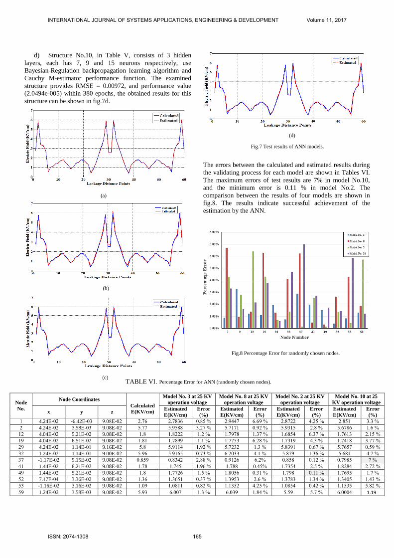
d) Structure No.10, in Table V, consists of 3 hidden
layers, each has 7, 9 and 15 neurons respectively, use
Bayesian-Regulation backpropagation learning algorithm and
Cauchy M-estimator performance function. The examined
structure provides RMSE = 0.00972, and performance value
(2.0494e-005) within 380 epochs, the obtained results for this
structure can be shown in fig.7d.
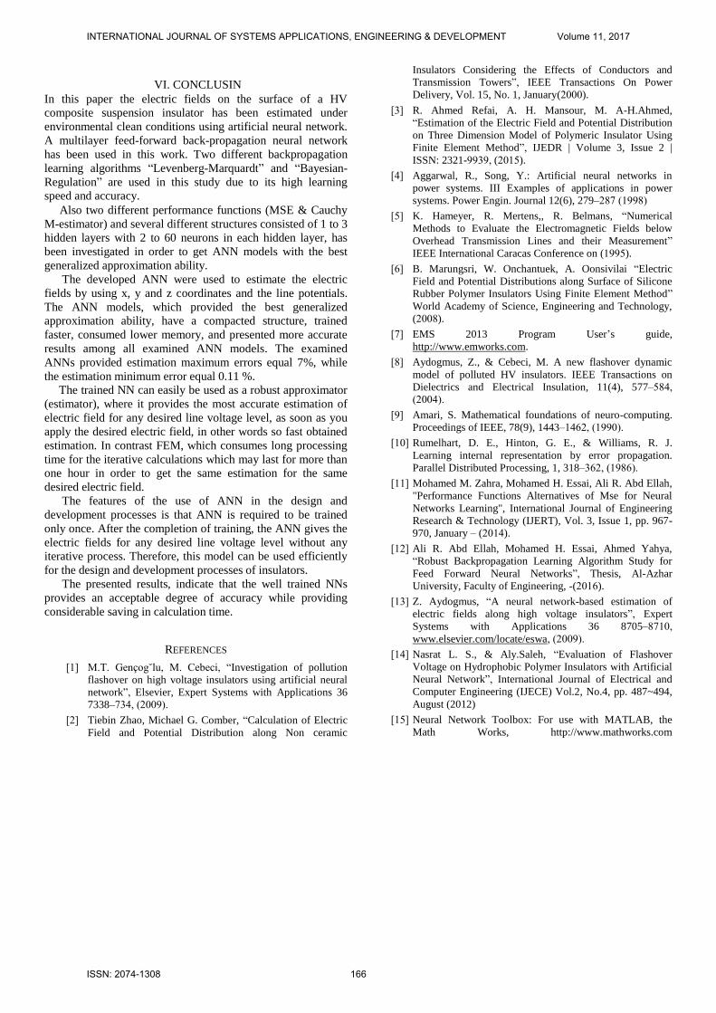
The errors between the calculated and estimated results during
the validating process for each model are shown in Tables VI.
The maximum errors of test results are 7% in model No.10,
and the minimum error is 0.11 % in model No.2. The
comparison between the results of four models are shown in
fig.8. The results indicate successful achievement of the
estimation by the ANN.
Node
No.
Node Coordinates
Calculated
E(KV/cm)
Model No. 3 at 25 KV
operation voltage
Model No. 8 at 25 KV
operation voltage
Model No. 2 at 25 KV
operation voltage
Model No. 10 at 25
KV operation voltage
x y z Estimated
E(KV/cm)
Error
(%)
Estimated
E(KV/cm)
Error
(%)
Estimated
E(KV/cm)
Error
(%)
Estimated
E(KV/cm)
Error
(%)
1 4.24E-02 -6.42E-03 9.08E-02 2.76 2.7836 0.85 % 2.9447 6.69 % 2.8722 4.25 % 2.851 3.3 %
2 4.24E-02 3.58E-03 9.08E-02 5.77 5.9588 3.27 % 5.7171 0.92 % 5.9315 2.8 % 5.6786 1.6 % 12 4.04E-02 5.21E-02 9.08E-02 1.8 1.8222 1.2 % 1.7978 1.37 % 1.6854 6.37 % 1.7613 2.15 % 19 4.04E-02 6.51E-02 9.08E-02 1.81 1.7899 1.1 % 1.7753 6.28 % 1.7319 4.3 % 1.7418 3.77 % 29 4.24E-02 1.14E-01 9.16E-02 5.8 5.9114 1.92 % 5.7232 1.3 % 5.8391 0.67 % 5.7657 0.59 % 32 1.24E-02 1.14E-01 9.00E-02 5.96 5.9165 0.73 % 6.2033 4.1 % 5.879 1.36 % 5.681 4.7 % 37 -1.17E-02 9.15E-02 9.08E-02 0.859 0.8342 2.88 % 0.9126 6.2% 0.858 0.12 % 0.7985 7 % 41 1.44E-02 8.21E-02 9.08E-02 1.78 1.745 1.96 % 1.788 0.45% 1.7354 2.5 % 1.8284 2.72 % 49 1.44E-02 5.21E-02 9.08E-02 1.8 1.7726 1.5 % 1.8056 0.31 % 1.798 0.11 % 1.7695 1.7 % 52 7.17E-04 3.36E-02 9.08E-02 1.36 1.3651 0.37 % 1.3953 2.6 % 1.3783 1.34 % 1.3405 1.43 % 53 -1.16E-02 3.16E-02 9.08E-02 1.09 1.0811 0.82 % 1.1352 4.25 % 1.0854 0.42 % 1.1535 5.82 % 59 1.24E-02 3.58E-03 9.08E-02 5.93 6.007 1.3 % 6.039 1.84 % 5.59 5.7 % 6.0004 1.19
Fig.8 Percentage Error for randomly chosen nodes.
Fig.7 Test results of ANN models.
TABLE VI. Percentage Error for ANN (randomly chosen nodes).
(a)
(b)
(c)
(d)
INTERNATIONAL JOURNAL OF SYSTEMS APPLICATIONS, ENGINEERING & DEVELOPMENT Volume 11, 2017
ISSN: 2074-1308 165
VI. CONCLUSIN
In this paper the electric fields on the surface of a HV
composite suspension insulator has been estimated under
environmental clean conditions using artificial neural network.
A multilayer feed-forward back-propagation neural network
has been used in this work. Two different backpropagation
learning algorithms “Levenberg-Marquardt” and “Bayesian-
Regulation” are used in this study due to its high learning
speed and accuracy.
Also two different performance functions (MSE & Cauchy
M-estimator) and several different structures consisted of 1 to 3
hidden layers with 2 to 60 neurons in each hidden layer, has
been investigated in order to get ANN models with the best
generalized approximation ability.
The developed ANN were used to estimate the electric
fields by using x, y and z coordinates and the line potentials.
The ANN models, which provided the best generalized
approximation ability, have a compacted structure, trained
faster, consumed lower memory, and presented more accurate
results among all examined ANN models. The examined
ANNs provided estimation maximum errors equal 7%, while
the estimation minimum error equal 0.11 %.
The trained NN can easily be used as a robust approximator
(estimator), where it provides the most accurate estimation of
electric field for any desired line voltage level, as soon as you
apply the desired electric field, in other words so fast obtained
estimation. In contrast FEM, which consumes long processing
time for the iterative calculations which may last for more than
one hour in order to get the same estimation for the same
desired electric field.
The features of the use of ANN in the design and
development processes is that ANN is required to be trained
only once. After the completion of training, the ANN gives the
electric fields for any desired line voltage level without any
iterative process. Therefore, this model can be used efficiently
for the design and development processes of insulators.
The presented results, indicate that the well trained NNs
provides an acceptable degree of accuracy while providing
considerable saving in calculation time.
REFERENCES
[1] M.T. Gençog˘lu, M. Cebeci, “Investigation of pollution
flashover on high voltage insulators using artificial neural
network”, Elsevier, Expert Systems with Applications 36
7338–734, (2009).
[2] Tiebin Zhao, Michael G. Comber, “Calculation of Electric
Field and Potential Distribution along Non ceramic
Insulators Considering the Effects of Conductors and
Transmission Towers”, IEEE Transactions On Power
Delivery, Vol. 15, No. 1, January(2000).
[3] R. Ahmed Refai, A. H. Mansour, M. A-H.Ahmed,
“Estimation of the Electric Field and Potential Distribution
on Three Dimension Model of Polymeric Insulator Using
Finite Element Method”, IJEDR | Volume 3, Issue 2 |
ISSN: 2321-9939, (2015).
[4] Aggarwal, R., Song, Y.: Artificial neural networks in
power systems. III Examples of applications in power
systems. Power Engin. Journal 12(6), 279–287 (1998)
[5] K. Hameyer, R. Mertens,, R. Belmans, “Numerical
Methods to Evaluate the Electromagnetic Fields below
Overhead Transmission Lines and their Measurement”
IEEE International Caracas Conference on (1995).
[6] B. Marungsri, W. Onchantuek, A. Oonsivilai “Electric
Field and Potential Distributions along Surface of Silicone
Rubber Polymer Insulators Using Finite Element Method”
World Academy of Science, Engineering and Technology,
(2008).
[7] EMS 2013 Program User’s guide,
http://www.emworks.com.
[8] Aydogmus, Z., & Cebeci, M. A new flashover dynamic
model of polluted HV insulators. IEEE Transactions on
Dielectrics and Electrical Insulation, 11(4), 577–584,
(2004).
[9] Amari, S. Mathematical foundations of neuro-computing.
Proceedings of IEEE, 78(9), 1443–1462, (1990).
[10] Rumelhart, D. E., Hinton, G. E., & Williams, R. J.
Learning internal representation by error propagation.
Parallel Distributed Processing, 1, 318–362, (1986).
[11] Mohamed M. Zahra, Mohamed H. Essai, Ali R. Abd Ellah,
"Performance Functions Alternatives of Mse for Neural
Networks Learning", International Journal of Engineering
Research & Technology (IJERT), Vol. 3, Issue 1, pp. 967-
970, January – (2014).
[12] Ali R. Abd Ellah, Mohamed H. Essai, Ahmed Yahya,
“Robust Backpropagation Learning Algorithm Study for
Feed Forward Neural Networks”, Thesis, Al-Azhar
University, Faculty of Engineering, -(2016).
[13] Z. Aydogmus, “A neural network-based estimation of
electric fields along high voltage insulators”, Expert
Systems with Applications 36 8705–8710,
www.elsevier.com/locate/eswa, (2009).
[14] Nasrat L. S., & Aly.Saleh, “Evaluation of Flashover
Voltage on Hydrophobic Polymer Insulators with Artificial
Neural Network”, International Journal of Electrical and
Computer Engineering (IJECE) Vol.2, No.4, pp. 487~494,
August (2012)
[15] Neural Network Toolbox: For use with MATLAB, the
Math Works, http://www.mathworks.com
INTERNATIONAL JOURNAL OF SYSTEMS APPLICATIONS, ENGINEERING & DEVELOPMENT Volume 11, 2017
ISSN: 2074-1308 166
Recommended