Download pdf - Network of European Union–funded collaborative research and development projects

Network of European Union–funded collaborative research and development projects

Michael J. Barber*Centro de Ciências Matemáticas, Universidade da Madeira, Funchal, Portugal

Andreas Krueger†

Fakultät für Physik, Universität Bielefeld, Bielefeld, Germany

Tyll Krueger‡

Fakultät für Physik, Universität Bielefeld, Bielefeld, Germany and Fachbereich Mathematik,Technische Universität Berlin, Berlin, Germany

Thomas Roediger-Schluga§

Department of Technology Policy, ARC Systems Research, Vienna, Austria�Received 20 October 2005; published 29 March 2006�

We describe collaboration networks consisting of research projects funded by the European Union �EU� andthe organizations involved in those projects. The networks are substantial in terms of size, complexity, andpotential impact on research policies and national economies in the EU. In empirical determinations of thenetwork properties, we observe characteristics similar to those of other collaboration networks, includingscale-free degree distributions, small diameter, and high clustering. We present some plausible models for theformation and structure of networks with the observed properties.

DOI: 10.1103/PhysRevE.73.036132 PACS number�s�: 89.75.Hc, 89.75.Da

I. INTRODUCTION

Real-world network analysis has recently become a majorresearch topic, following the landmark work of Watts andStrogatz �1�. Most prominent are perhaps the investigationsof the structure of the World Wide Web, the network of in-ternet routers, and certain social networks like citation net-works. On the theoretical side, one tries to understand themechanisms of formation of such networks and to derivestatistical properties of the networks from the generatingrules. On the rigorous mathematical side, there are only afew results for specific models, indicating the difficulty of apurely mathematical approach �for a survey of recent resultsin this direction, see �2��. Thus, the main approach is to usesome mean field assumption to get relevant informationabout the corresponding graphs. Although it is not clearwhere the limits of this approach lie, in many cases the re-sults match well with numerical simulations and empiricaldata. Several useful reviews of recent research in networksare available, such as �3�.

In this paper, we study a particular collaboration network.Its vertices are research projects funded by the EuropeanUnion �EU� and the organizations involved in those projects.In total, the database contains over 20 000 projects and35 000 participating organizations. The network shows allthe main characteristics known from other complex networkstructures, such as scale-free degree distribution, small diam-

eter, high clustering, and assortative vertex correlations.Besides the general interest in studying a new, real-world

network of large size and high complexity, the study couldhave a significant economic impact. Improving collaborationbetween actors involved in innovation processes is a keyobjective of current science, technology, and innovationpolicy in industrialized countries. However, little is knownabout what kind of network structures emerge from suchinitiatives. Moreover, it is quite likely that network structureaffects network functions such as knowledge creation,knowledge diffusion, and the collaboration of particulartypes of actors. Presumably, this is determined by both en-dogenous formation mechanisms and exogenous frameworkconditions. In order to progress in our understanding, it istherefore essential to have sound statistics on the structure ofnetworks we observe and to develop plausible models ofhow these are formed and evolve over time.

The model networks we use to compare with the empiri-cal data are random intersection graphs, a natural frameworkfor describing projections of bipartite graphs. Discrete inter-section graphs similar to the ones we use were first discussedin �4�. We extend and refine the construction from �4� to bemore applicable to real-world graphs.

Perhaps the most important finding from our model ap-proach is the strong determination of the real network struc-ture by the degree distribution. That is, most statistical prop-erties we measure in the EU research project networks arethe ones observed in a typical realization of a uniformweighted random graph model with given �bipartite� degreedistribution as in the EU networks. Since this distribution ischaracterized by two exponents—one for each partition—wehave essentially only four parameters �size, edge number,and exponents� which are needed to describe the entire net-work. This tremendous reduction of complexity indicates

*Electronic address: [email protected]†Electronic address: [email protected]‡Electronic address: [email protected]§Electronic address: [email protected]

PHYSICAL REVIEW E 73, 036132 �2006�

1539-3755/2006/73�3�/036132�13�/$23.00 ©2006 The American Physical Society036132-1

http://dx.doi.org/10.1103/PhysRevE.73.036132

that only a few basic formation rules are driving the networkevolution.

In Sec. II, we describe the preparation of the data on theEU research programs. We present empirical determinationof the network properties in Sec. III, followed by an expla-nation of these properties using a random intersection graphmodel in Sec. IV. Finally, in Sec. V, we summarize the keyresults and consider implications of the network propertieson EU research programs.

II. THE DATA SET

In this work, we study research collaboration networksthat have emerged in the European Union’s successive four-year Framework Programs �FPs� on Research and Techno-logical Development. Since their inception in 1984, six FPshave been launched, on the first four of which we have com-prehensive data. FPs are organized in priority areas, whichinclude information and communication technologies �ICTs�,energy, industrial technologies, life sciences, environment,transportation, and a number of additional activities. In linewith economic structural change, the main thematic focus ofthe FPs has shifted somewhat over time from energy andindustrial technologies to the application of ICTs and lifesciences. The majority of funding activities are aimed atstimulating research partnerships between firms, universities,research organizations, governmental actors, nongovernmen-tal organizations, lobby groups, etc. Since FP4, the scope ofactivities has been expanded to also cover training, network-ing, demonstration, and preparatory activities �for details, seeRef. �5��. In order to keep our data set compatible over thedifferent FPs, we have excluded the latter set of projectsfrom FP4 and focus only on collaborative research projects�see Table I�.

In order to receive funding, projects in FP1–FP4 had tocomprise at least two organizations from at least two mem-ber states. We have retrieved data on these projects from thepublicly available Community Research and DevelopmentInformation Service �CORDIS� projects database �6�. Thisdatabase contains information on all funded projects as wellas a reasonably complete listing of all participating organi-zations.

The raw data on participating organizations are rather in-consistent. Apart from incoherent spelling in up to four lan-guages per country, organizations are labeled inhomoge-neously. Entries may range from large corporate groupings,such as Siemens, or large public research organizations, likethe Spanish CSIC, to individual departments or laboratories,and are listed as valid at the time the respective project wascarried out. Among heterogeneous organizations, only a sub-set contains information on the unit actually participating oron geographical location. Information on older entries andthe substructure of firms tends to be less complete.

Because of these difficulties, any automatic standardiza-tion method akin to the one utilized by Newman �7� is inap-propriate to this kind of data. Rather, the raw data have to becleaned and completed manually, which is an ongoingproject at ARC Systems Research. The objective of this workis to produce a data set useful for policy advice by identify-ing homogeneous, economically meaningful organizationalentities. To this end, organizational boundaries are defined bylegal control and entries are assigned to the respective orga-nizations. Resulting heterogeneous organizations, such asuniversities, large research centers, or conglomerate firms arebroken down into subentities that operate in fairly coherentareas of activity, such as faculties, institutes, divisions, orsubsidiaries. These can be identified for a large number ofentries, based on the available contact information of partici-pants, and are comparable across organizations.

The case of the French Centre National de la RechercheScientifique �CNRS�, the most active participant in the EUFPs, may serve as an illustration. First, 785 separate entrieswere summarized under a unique organizational label. Next,these 785 entries were broken down into the eight areas ofresearch activity in which CNRS is currently organized.Based on available information on participating units andgeographical location, 732 of the 785 entries could be as-signed to one of these subentities. For the remaining 53 en-tries, the nonspecific label CNRS was used.

Comparable success rates were achieved for other largepublic research organizations and universities. Due to scarcerinformation, firms could not be broken down at a comparablerate. Moreover, due to resource constraints, standardizationwork has focused on the major players in the FPs. Organiza-tions participating in fewer than a total of 30 projects in

TABLE I. FP1–FP4 total budget and number of funded projects. The smaller average funding per projectand organization in FP4 is an artifact as it involves a large number of scholarships and the like, which aresmaller than research projects �however, we cannot isolate the bias created�.

Framework Program Budgeta No. of PMillionEuros/P

No. of�P�1�b

No. ofO

MillionEuros/O

FP1 �1984–1988� 3.8 3283 1.15 1696 2500 1.52

FP2 �1987–1991� 5.4 3885 1.39 3013 6135 0.88

FP3 �1990–1994� 6.65 5294 1.25 4611 9615 0.69

FP4c �1994–1998� 13.3 15061 �9087� 0.88 11374 �8039� 20873 0.64

aBillion Euros.bProjects with more then one participating organization.cResearch and development projects listed in parentheses. The number excludes all projects devoted topreparatory, demonstration, and training activities.

BARBER et al. PHYSICAL REVIEW E 73, 036132 �2006�

036132-2

FP1–FP4 have not been broken down yet. Due to these limi-tations in processing the data, we cannot rule out the possi-bility of a bias in analyzing our data. However, we have runall the reported analyses with the undivided organizationsand have obtained qualitatively similar results, apart fromdifferent extreme values, e.g., maximum degree.

Table I displays information on the present data set, whichcontains information on a total of 27 758 projects, carried outover the period 1984–2004. It shows that the total budget aswell as number of funded projects has increased dramaticallyfrom FP1 to FP4. Moreover, it provides a rough measure onthe completeness of the available data. For a sizable numberof projects, the CORDIS project database lists informationonly on the project coordinator. This is due to the age of thedata and inhomogeneous disclosure policies of different unitsat the European Commission. Comparing the number ofprojects containing information on more than one participantwith the total number of projects funded in each FP showsthat the data are fairly complete as of FP2.

The facts that FP1 was the first program launched and thatthe available data are rather incomplete make it exceptionalin many respects. We therefore focus our analyses on FP2–FP4 and only give graph characteristic values for FP1 toindicate the difference from the networks created by the sub-sequent FPs.

III. THE NETWORK STRUCTURE

In this section, we present the basic properties of the net-work structure for projects and organizations in the first four

EU Framework Programs. We consider both graphs as inter-section graphs �4�, each being the dual of the other, which,for our purposes, is generally more convenient than the usualbipartite-graph point of view. The vertices of an intersectiongraph are given by an enumerated collection of sets withelements from a given fixed base-set, while the edges aredefined via an intersection property �edge � nonempty inter-section of two sets�. The sets need not be distinct.

We denote by P= �P1 ; . . . ; PM� the family of projects andby O= �O1 ; . . . ;ON� the family of organizations. Projects areunderstood as labeled sets of organizations and organizationsas labeled sets of projects. The corresponding intersectiongraphs are denoted by GP and GO; we will also use the termsP graph and O graph for them. The size �x� of a vertex x fromGP or GO is the cardinality of the set corresponding to thevertex; in the picture of bipartite graphs, the size is just thedegree of the vertex. In Tables II and III, we give some basicparameters measured on the P and O graphs from the fourFramework Programs. Since the degree distribution for Pgraphs is a superposition of two power-law distributions �onefor small degree values and one for large values�, we give thecorresponding values for the exponents parenthetically. Theclustering coefficients shown are defined �following �1�� asfollows. Assume that vertex v has dv neighbors; potentially,dv�dv−1� /2 edges could exist between those neighbors,forming triangles. Define an auxiliary, vertex-specific clus-tering coefficient Cv as the ratio of the number of those tri-angles actually formed to the number of triangles that poten-tially could be formed. The clustering coefficient for the

TABLE II. Basic network properties of FP1–FP4 organizations projection.

Graph characteristic FP1 FP2 FP3 FP4

No. of vertices N 2500 6135 9615 20873

�N for largest component� �2038� �5875� �8920� �20130�N outside largest component 462 260 695 743

No. of edges M 9557 64300 113693 199965

�No. of edges M largest component� �9410� �64162� �113219� �199182�

Mean degree d̄ 7.65 20.96 23.65 19.16

�d̄ largest component� �9.23� �21.84� �25.39� �19.79�

Maximal degree dmax 140 386 648 649

Mean triangles per vertex � 22.90 169.70 244.91 146.04

�� largest component� �27.97� 177.16 263.84 151.26

Maximal triangle number 966 5295 15128 10730

Cluster coefficient C̄ 0.57 0.72 0.72 0.79

�C̄ largest component� �0.67� �0.74� �0.75� �0.81�

Number of components 369 183 455 467

Diameter of largest component 9 7 9 10

Mean path length � of largest component 3.70 3.27 3.32 3.59

Exponent of degree distribution −2.1 −2.0 −2.0 −2.1

Variance of degree exponent 0.4 0.3 0.3 0.3

Exponent of organization size distribution −2.1 −1.9 −1.7 −1.8

Variance of size exponent 0.5 0.3 0.5 0.3

Mean no. of projects per organization E��O � � 2.40 4. 87 5.6 6.24

Maximal size �max�O�� 130 82 138 172

NETWORK OF EUROPEAN UNION–FUNDED¼ PHYSICAL REVIEW E 73, 036132 �2006�

036132-3

network as a whole is just the average of Cv over all verticesin the graph.

As expected, FP1–FP4 are of small-world type: high clus-tering coefficient and small diameter of the giant component.There is a slight increase in the clustering coefficient of theO graphs from FP1 to FP4, indicating a stronger integrationamong groups of collaborating organizations. This is alsoreflected in the mean organization size which increases from2.4 to 6.2. There is an interesting jump in the P graph meandegree values and the mean triangle numbers between FP1and FP2 and between FP2 and FP3. The maximal degrees ofthe O graphs are high in comparison with the mean degrees,which is a consequence of the power-law degree structure.For the P graphs, the gap between mean and maximal degreeis less pronounced.

More information is contained in the statistical propertiesof the relevant distributions. The numerical data strongly in-dicate that the size distributions follow power laws. Also, theO graph degree distribution is of power-law type, while theproject-graph degree distribution is a superposition of twoscale-free distributions, one dominating the distribution forsmall degree values �up to 100� and one relevant for the largedegree values. We discuss these properties at greater lengthin the following sections.

A. Size distributions

The size distributions are the basic distributions for theEU networks since, as will be shown in Sec. IV B, a typical

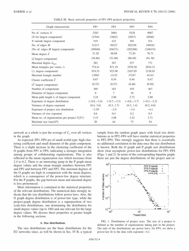
sample from the random graph space with fixed size distri-butions as in FP2–FP4 will have similar statistical propertiesto FP2–FP4. This strongly suggests that there is essentiallyno additional correlation in the data once the size distributionis known. Both the O graph and P graph size distributionsshow clear asymptotic power-law distributions for FP1–FP4�Figs. 1 and 2�. In terms of the corresponding bipartite graph,these are just the degree distributions of the project and or-

TABLE III. Basic network properties of FP1–FP4 projects projection.

Graph characteristic FP1 FP2 FP3 FP4

No of. vertices N 3283 3884 5528 9087

�N for largest component� �2764� �3662� �5027� �8566�N outside largest component 519 222 501 521

No. of edges M 51217 94527 202358 348542

�No of. edges M largest component� �50940� �94471� �202306� �348474�

Mean degree d̄ 31.20 48.68 73.20 76.71

�d̄ largest component� �36.86� �51.60� �80.49� �81.36�

Maximal degree dmax 282 387 917 771

Mean triangles per vertex � 774.41 871.19 1970.30 2034.31

�� largest component� 919.53 923.98 2167.05 2158.03

Maximal triangle number 12903 11125 37247 41141

Cluster coefficient C̄ 0.67 0.54 0.44 0.47

�C̄ largest component� �0.75� �0.57� �0.48� �0.50�

Number of components 369 183 455 467

Diameter of largest component 9 7 10 9

Mean path length � of largest component 3.24 2.80 2.72 2.80

Exponent of degree distribution �−0.8,−3.4� �−0.7,−3.3� �−0.6,−3.7� �−0.3,−2.2�Variance of degree exponent �0.4, 3.6� �0.3, 1.7� �0.3, 1.4� �0.2, 0.6�Exponent of project size distrbution −3.59 −2.9 −3.4 −4.1

Variance of size exponent 0.6 0.4 0.2 0.3

Mean no. of organizations per project E��P � � 3.15 3.08 3.22 2.71

Maximal size �max�P�� 20 44 73 54

FIG. 1. Distribution of project sizes. The size of a project isdefined as the number of organizations taking part in the project.The tails of the distributions are power laws; for FP4, we show apower-law fit to the data with exponent −4.1.


036132-4

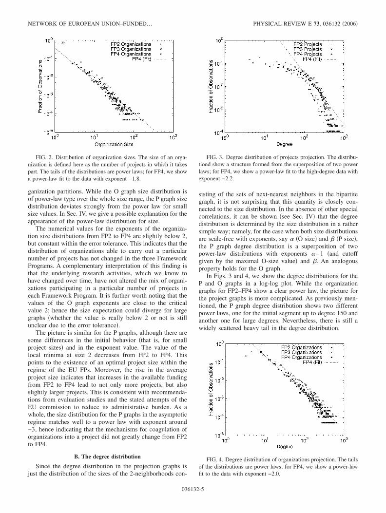
ganization partitions. While the O graph size distribution isof power-law type over the whole size range, the P graph sizedistribution deviates strongly from the power law for smallsize values. In Sec. IV, we give a possible explanation for theappearance of the power-law distribution for size.

The numerical values for the exponents of the organiza-tion size distributions from FP2 to FP4 are slightly below 2,but constant within the error tolerance. This indicates that thedistribution of organizations able to carry out a particularnumber of projects has not changed in the three FrameworkPrograms. A complementary interpretation of this finding isthat the underlying research activities, which we know tohave changed over time, have not altered the mix of organi-zations participating in a particular number of projects ineach Framework Program. It is further worth noting that thevalues of the O graph exponents are close to the criticalvalue 2; hence the size expectation could diverge for largegraphs �whether the value is really below 2 or not is stillunclear due to the error tolerance�.

The picture is similar for the P graphs, although there aresome differences in the initial behavior �that is, for smallproject sizes� and in the exponent value. The value of thelocal minima at size 2 decreases from FP2 to FP4. Thispoints to the existence of an optimal project size within theregime of the EU FPs. Moreover, the rise in the averageproject size indicates that increases in the available fundingfrom FP2 to FP4 lead to not only more projects, but alsoslightly larger projects. This is consistent with recommenda-tions from evaluation studies and the stated attempts of theEU commission to reduce its administrative burden. As awhole, the size distribution for the P graphs in the asymptoticregime matches well to a power law with exponent around−3, hence indicating that the mechanisms for coagulation oforganizations into a project did not greatly change from FP2to FP4.

B. The degree distribution

Since the degree distribution in the projection graphs isjust the distribution of the sizes of the 2-neighborhoods con-

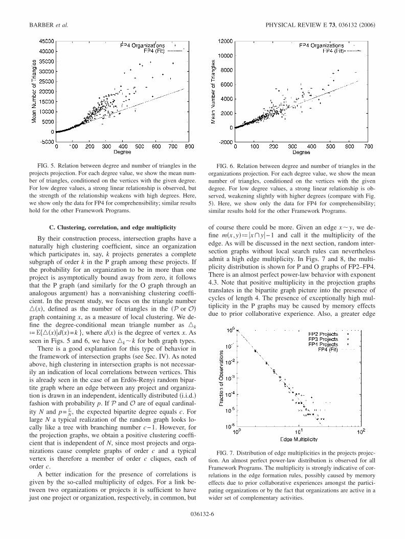
sisting of the sets of next-nearest neighbors in the bipartitegraph, it is not surprising that this quantity is closely con-nected to the size distribution. In the absence of other specialcorrelations, it can be shown �see Sec. IV� that the degreedistribution is determined by the size distribution in a rathersimple way; namely, for the case when both size distributionsare scale-free with exponents, say � �O size� and � �P size�,the P graph degree distribution is a superposition of twopower-law distributions with exponents �−1 �and cutoffgiven by the maximal O-size value� and �. An analogousproperty holds for the O graph.

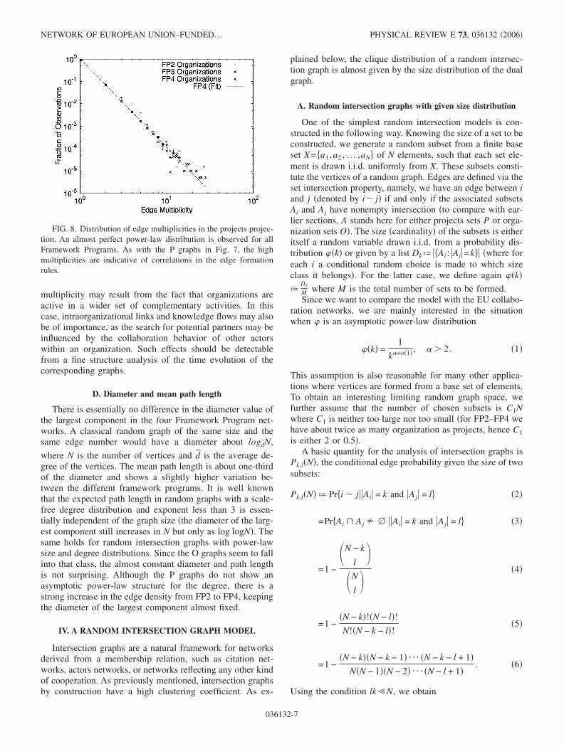
In Figs. 3 and 4, we show the degree distributions for theP and O graphs in a log-log plot. While the organizationgraphs for FP2–FP4 show a clear power law, the picture forthe project graphs is more complicated. As previously men-tioned, the P graph degree distribution shows two differentpower laws, one for the initial segment up to degree 150 andanother one for large degrees. Nevertheless, there is still awidely scattered heavy tail in the degree distribution.

FIG. 2. Distribution of organization sizes. The size of an orga-nization is defined here as the number of projects in which it takespart. The tails of the distributions are power laws; for FP4, we showa power-law fit to the data with exponent −1.8.

FIG. 3. Degree distribution of projects projection. The distribu-tiond show a structure formed from the superposition of two powerlaws; for FP4, we show a power-law fit to the high-degree data withexponent −2.2.

FIG. 4. Degree distribution of organizations projection. The tailsof the distributions are power laws; for FP4, we show a power-lawfit to the data with exponent −2.0.


036132-5

C. Clustering, correlation, and edge multiplicity

By their construction process, intersection graphs have anaturally high clustering coefficient, since an organizationwhich participates in, say, k projects generates a completesubgraph of order k in the P graph among these projects. Ifthe probability for an organization to be in more than oneproject is asymptotically bound away from zero, it followsthat the P graph �and similarly for the O graph through ananalogous argument� has a nonvanishing clustering coeffi-cient. In the present study, we focus on the triangle number��x�, defined as the number of triangles in the �P or O�graph containing x, as a measure of local clustering. We de-fine the degree-conditional mean triangle number as �kªE��x��d�x�=k��, where d�x� is the degree of vertex x. Asseen in Figs. 5 and 6, we have �k�k for both graph types.

There is a good explanation for this type of behavior inthe framework of intersection graphs �see Sec. IV�. As notedabove, high clustering in intersection graphs is not necessar-ily an indication of local correlations between vertices. Thisis already seen in the case of an Erdös-Renyi random bipar-tite graph where an edge between any project and organiza-tion is drawn in an independent, identically distributed �i.i.d.�fashion with probability p. If P and O are of equal cardinal-ity N and p= c

N , the expected bipartite degree equals c. Forlarge N a typical realization of the random graph looks lo-cally like a tree with branching number c−1. However, forthe projection graphs, we obtain a positive clustering coeffi-cient that is independent of N, since most projects and orga-nizations cause complete graphs of order c and a typicalvertex is therefore a member of order c cliques, each oforder c.

A better indication for the presence of correlations isgiven by the so-called multiplicity of edges. For a link be-tween two organizations or projects it is sufficient to havejust one project or organization, respectively, in common, but

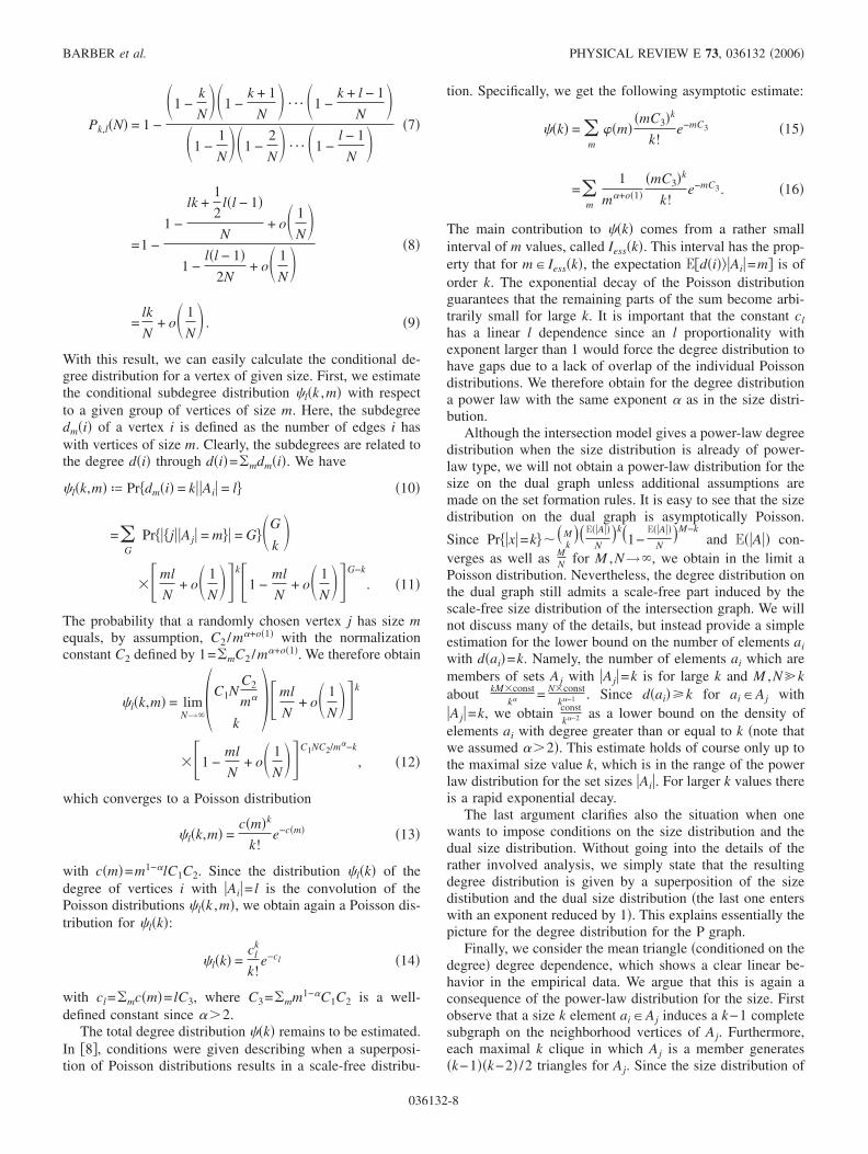
of course there could be more. Given an edge x�y, we de-fine m�x ,y�ª �x�y�−1 and call it the multiplicity of theedge. As will be discussed in the next section, random inter-section graphs without local search rules can neverthelessadmit a high edge multiplicity. In Figs. 7 and 8, the multi-plicity distribution is shown for P and O graphs of FP2–FP4.There is an almost perfect power-law behavior with exponent4.3. Note that positive multiplicity in the projection graphstranslates in the bipartite graph picture into the presence ofcycles of length 4. The presence of exceptionally high mul-tiplicity in the P graphs may be caused by memory effectsdue to prior collaborative experience. Also, a greater edge

FIG. 5. Relation between degree and number of triangles in theprojects projection. For each degree value, we show the mean num-ber of triangles, conditioned on the vertices with the given degree.For low degree values, a strong linear relationship is observed, butthe strength of the relationship weakens with high degrees. Here,we show only the data for FP4 for comprehensibility; similar resultshold for the other Framework Programs.

FIG. 6. Relation between degree and number of triangles in theorganizations projection. For each degree value, we show the meannumber of triangles, conditioned on the vertices with the givendegree. For low degree values, a strong linear relationship is ob-served, weakening slightly with higher degrees �compare with Fig.5�. Here, we show only the data for FP4 for comprehensibility;similar results hold for the other Framework Programs.

FIG. 7. Distribution of edge multiplicities in the projects projec-tion. An almost perfect power-law distribution is observed for allFramework Programs. The multiplicity is strongly indicative of cor-relations in the edge formation rules, possibly caused by memoryeffects due to prior collaborative experiences amongst the partici-pating organizations or by the fact that organizations are active in awider set of complementary activities.


036132-6

multiplicity may result from the fact that organizations areactive in a wider set of complementary activities. In thiscase, intraorganizational links and knowledge flows may alsobe of importance, as the search for potential partners may beinfluenced by the collaboration behavior of other actorswithin an organization. Such effects should be detectablefrom a fine structure analysis of the time evolution of thecorresponding graphs.

D. Diameter and mean path length

There is essentially no difference in the diameter value ofthe largest component in the four Framework Program net-works. A classical random graph of the same size and thesame edge number would have a diameter about logd̄N,

where N is the number of vertices and d̄ is the average de-gree of the vertices. The mean path length is about one-thirdof the diameter and shows a slightly higher variation be-tween the different framework programs. It is well knownthat the expected path length in random graphs with a scale-free degree distribution and exponent less than 3 is essen-tially independent of the graph size �the diameter of the larg-est component still increases in N but only as log logN�. Thesame holds for random intersection graphs with power-lawsize and degree distributions. Since the O graphs seem to fallinto that class, the almost constant diameter and path lengthis not surprising. Although the P graphs do not show anasymptotic power-law structure for the degree, there is astrong increase in the edge density from FP2 to FP4, keepingthe diameter of the largest component almost fixed.

IV. A RANDOM INTERSECTION GRAPH MODEL

Intersection graphs are a natural framework for networksderived from a membership relation, such as citation net-works, actors networks, or networks reflecting any other kindof cooperation. As previously mentioned, intersection graphsby construction have a high clustering coefficient. As ex-

plained below, the clique distribution of a random intersec-tion graph is almost given by the size distribution of the dualgraph.

A. Random intersection graphs with given size distribution

One of the simplest random intersection models is con-structed in the following way. Knowing the size of a set to beconstructed, we generate a random subset from a finite baseset X= �a1 ,a2 , . . . ,aN� of N elements, such that each set ele-ment is drawn i.i.d. uniformly from X. These subsets consti-tute the vertices of a random graph. Edges are defined via theset intersection property, namely, we have an edge between iand j �denoted by i� j� if and only if the associated subsetsAi and Aj have nonempty intersection �to compare with ear-lier sections, A stands here for either projects sets P or orga-nization sets O�. The size �cardinality� of the subsets is eitheritself a random variable drawn i.i.d. from a probability dis-tribution ��k� or given by a list Dkª ��Ai : �Ai�=k�� where foreach i a conditional random choice is made to which sizeclass it belongs�. For the latter case, we define again ��k�ª

Dk

M where M is the total number of sets to be formed.Since we want to compare the model with the EU collabo-

ration networks, we are mainly interested in the situationwhen � is an asymptotic power-law distribution

��k� =1

k�+o�1� , � � 2. �1�

This assumption is also reasonable for many other applica-tions where vertices are formed from a base set of elements.To obtain an interesting limiting random graph space, wefurther assume that the number of chosen subsets is C1Nwhere C1 is neither too large nor too small �for FP2–FP4 wehave about twice as many organization as projects, hence C1is either 2 or 0.5�.

A basic quantity for the analysis of intersection graphs isPk,l�N�, the conditional edge probability given the size of twosubsets:

Pk,l�N� ª Pr�i � j��Ai� = k and �Aj� = l� �2�

=Pr�Ai � Aj � � ��Ai� = k and �Aj� = l� �3�

=1 −N − k

l

N

l �4�

=1 −�N − k�!�N − l�!N!�N − k − l�!

�5�

=1 −�N − k��N − k − 1� ¯ �N − k − l + 1�

N�N − 1��N − 2� ¯ �N − l + 1�. �6�

Using the condition lk�N, we obtain

FIG. 8. Distribution of edge multiplicities in the projects projec-tion. An almost perfect power-law distribution is observed for allFramework Programs. As with the P graphs in Fig. 7, the highmultiplicities are indicative of correlations in the edge formationrules.


036132-7

Pk,l�N� = 1 −1 −

k

N1 −

k + 1

N¯ 1 −

k + l − 1

N

1 −1

N1 −

2

N¯ 1 −

l − 1

N �7�

=1 −

1 −

lk +1

2l�l − 1�

N+ o 1

N

1 −l�l − 1�

2N+ o 1

N �8�

=lk

N+ o 1

N . �9�

With this result, we can easily calculate the conditional de-gree distribution for a vertex of given size. First, we estimatethe conditional subdegree distribution �l�k ,m� with respectto a given group of vertices of size m. Here, the subdegreedm�i� of a vertex i is defined as the number of edges i haswith vertices of size m. Clearly, the subdegrees are related tothe degree d�i� through d�i�=�mdm�i�. We have

�l�k,m� ª Pr�dm�i� = k��Ai� = l� �10�

=�G

Pr��j��Aj� = m�� = G�G

k

��ml

N+ o 1

N k�1 −

ml

N+ o 1

N G−k

. �11�

The probability that a randomly chosen vertex j has size mequals, by assumption, C2 /m�+o�1� with the normalizationconstant C2 defined by 1=�mC2 /m�+o�1�. We therefore obtain

�l�k,m� = limN→�C1N

C2

m�

k��ml

N+ o 1

N k

��1 −ml

N+ o 1

N C1NC2/m�−k

, �12�

which converges to a Poisson distribution

�l�k,m� =c�m�k

k!e−c�m� �13�

with c�m�=m1−�lC1C2. Since the distribution �l�k� of thedegree of vertices i with �Ai�= l is the convolution of thePoisson distributions �l�k ,m�, we obtain again a Poisson dis-tribution for �l�k�:

�l�k� =cl

k

k!e−cl �14�

with cl=�mc�m�= lC3, where C3=�mm1−�C1C2 is a well-defined constant since ��2.

The total degree distribution ��k� remains to be estimated.In �8�, conditions were given describing when a superposi-tion of Poisson distributions results in a scale-free distribu-

tion. Specifically, we get the following asymptotic estimate:

��k� = �m

��m��mC3�k

k!e−mC3 �15�

=�m

1

m�+o�1��mC3�k

k!e−mC3. �16�

The main contribution to ��k� comes from a rather smallinterval of m values, called Iess�k�. This interval has the prop-erty that for m� Iess�k�, the expectation E�d�i��Ai�=m� is oforder k. The exponential decay of the Poisson distributionguarantees that the remaining parts of the sum become arbi-trarily small for large k. It is important that the constant clhas a linear l dependence since an l proportionality withexponent larger than 1 would force the degree distribution tohave gaps due to a lack of overlap of the individual Poissondistributions. We therefore obtain for the degree distributiona power law with the same exponent � as in the size distri-bution.

Although the intersection model gives a power-law degreedistribution when the size distribution is already of power-law type, we will not obtain a power-law distribution for thesize on the dual graph unless additional assumptions aremade on the set formation rules. It is easy to see that the sizedistribution on the dual graph is asymptotically Poisson.

Since Pr��x�=k�� Mk

��E��A��

N�k�1−

E��A��

N�M−k

and E��A�� con-verges as well as M

N for M ,N→, we obtain in the limit aPoisson distribution. Nevertheless, the degree distribution onthe dual graph still admits a scale-free part induced by thescale-free size distribution of the intersection graph. We willnot discuss many of the details, but instead provide a simpleestimation for the lower bound on the number of elements aiwith d�ai�=k. Namely, the number of elements ai which aremembers of sets Aj with �Aj�=k is for large k and M ,Nkabout kM�const

k� = N�constk�−1 . Since d�ai��k for ai�Aj with

�Aj�=k, we obtain constk�−2 as a lower bound on the density of

elements ai with degree greater than or equal to k �note thatwe assumed ��2�. This estimate holds of course only up tothe maximal size value k, which is in the range of the powerlaw distribution for the set sizes �Ai�. For larger k values thereis a rapid exponential decay.

The last argument clarifies also the situation when onewants to impose conditions on the size distribution and thedual size distribution. Without going into the details of therather involved analysis, we simply state that the resultingdegree distribution is given by a superposition of the sizedistibution and the dual size distribution �the last one enterswith an exponent reduced by 1�. This explains essentially thepicture for the degree distribution for the P graph.

Finally, we consider the mean triangle �conditioned on thedegree� degree dependence, which shows a clear linear be-havior in the empirical data. We argue that this is again aconsequence of the power-law distribution for the size. Firstobserve that a size k element ai�Aj induces a k−1 completesubgraph on the neighborhood vertices of Aj. Furthermore,each maximal k clique in which Aj is a member generates�k−1��k−2� /2 triangles for Aj. Since the size distribution of


036132-8

the elements ai is Poisson with expectation of, say, c and thedegree of Aj is proportional to the size �Aj�, we obtain for theconditional expected number of triangles �k given the de-gree k:

�k ª E�number of triangles containing A�d�A� = k�

�c2

2const � k . �17�

In deriving Eq. �17�, we used the facts that with high prob-ability the size of the intersection between two sets Ai and Ajhas cardinality 1 �conditioned on the two sets having a non-empty intersection� and that the Poisson distribution has anexponentially decaying tail.

B. A Molloy-Reed version of random intersection graphs anda Bernoulli-type model

We sketch the construction of random intersection graphswith given size distribution � and size distribution � on thedual. The two distributions are not independent but mustsatisfy the condition �ii��i�=�ii��i�. There are further re-strictions on the maximal size in order to get a reasonablerandom graph model. Note that the problem is equivalent tothe construction of a random bipartite graph given the degreesequence on the two partitions. The approach we follow is avariation of the graph construction algorithm usually attrib-

uted to Molloy and Reed �9� �actually given earlier by Bol-lobás �10��.

Assign first to each set A and each element a from thebase set a random size value according to the given distribu-tions � and �. Let Dk be the resulting set of elements ai withsize k. Replace each element from Dk by k virtual elementsai,l , l=1,2 , . . . ,k and form a new base set X� with all thevirtual elements. The set formation process for the sets �Ai� isnow the same as in the previous section except that eachchosen virtual element ai,l will be removed from X� when itwas selected first into a set. After the sets are constructed weidentify the virtual elements back into the original ones, re-move multiple and self-links, and define the correspondingset graph in the usual way.

By construction the resulting size distribution on the dualgraph will be given by � as long as the probability of choos-ing two virtual elements ai,l and ai,m �corresponding to thesame element ai� is sufficiently small. To ensure this one hasto impose restrictions on the maximal size values. It is notdifficult to show that the correlation between the size of Aand the size of an element a is multiplicative. In case of alinear relation between the number of sets N and the numberof elements M we have

Pr�a � A��A� = k and �a� = l� �const

Nkl . �18�

To see this observe that

Pr�a � A��A� = k and �a� = l� = 1 − Pr�among the k choices to generate A is no virtual a element� �19�

=1 −M* − l

M*

M* − 1 − l

M* − 1¯

M* − k − l + 1

M* − k + 1�20�

with M* being the number of virtual elements. The last for-mula has the same structure as the expression for the pairingprobability in the previous section, hence we get, forlk�M* and bounded first moments of the � distribution,the claimed multiplicative correlation. We note that there isalso a variant of the Molloy-Reed construction whichproduces an additive size-size correlation such thatPr�a� �A��A�=k and �a�= l�� const

N �k+ l� holds �see �11� fordetails of the algorithm�.

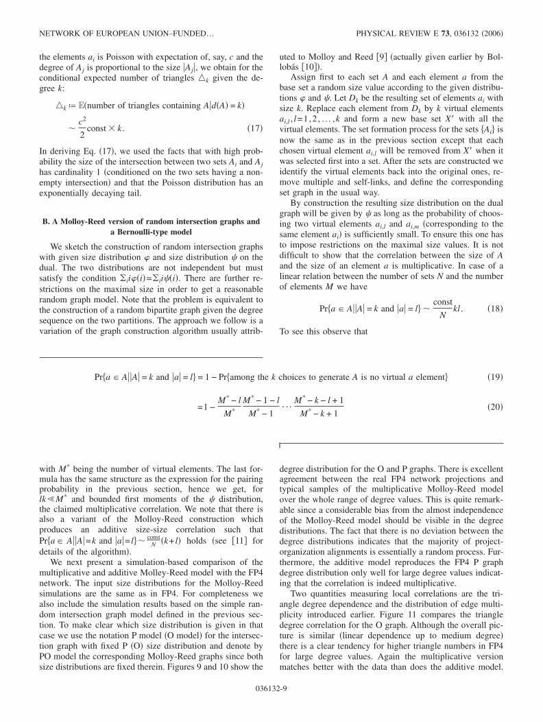
We next present a simulation-based comparison of themultiplicative and additive Molley-Reed model with the FP4network. The input size distributions for the Molloy-Reedsimulations are the same as in FP4. For completeness wealso include the simulation results based on the simple ran-dom intersection graph model defined in the previous sec-tion. To make clear which size distribution is given in thatcase we use the notation P model �O model� for the intersec-tion graph with fixed P �O� size distribution and denote byPO model the corresponding Molloy-Reed graphs since bothsize distributions are fixed therein. Figures 9 and 10 show the

degree distribution for the O and P graphs. There is excellentagreement between the real FP4 network projections andtypical samples of the multiplicative Molloy-Reed modelover the whole range of degree values. This is quite remark-able since a considerable bias from the almost independenceof the Molloy-Reed model should be visible in the degreedistributions. The fact that there is no deviation between thedegree distributions indicates that the majority of project-organization alignments is essentially a random process. Fur-thermore, the additive model reproduces the FP4 P graphdegree distribution only well for large degree values indicat-ing that the correlation is indeed multiplicative.

Two quantities measuring local correlations are the tri-angle degree dependence and the distribution of edge multi-plicity introduced earlier. Figure 11 compares the triangledegree correlation for the O graph. Although the overall pic-ture is similar �linear dependence up to medium degree�there is a clear tendency for higher triangle numbers in FP4for large degree values. Again the multiplicative versionmatches better with the data than does the additive model.


036132-9

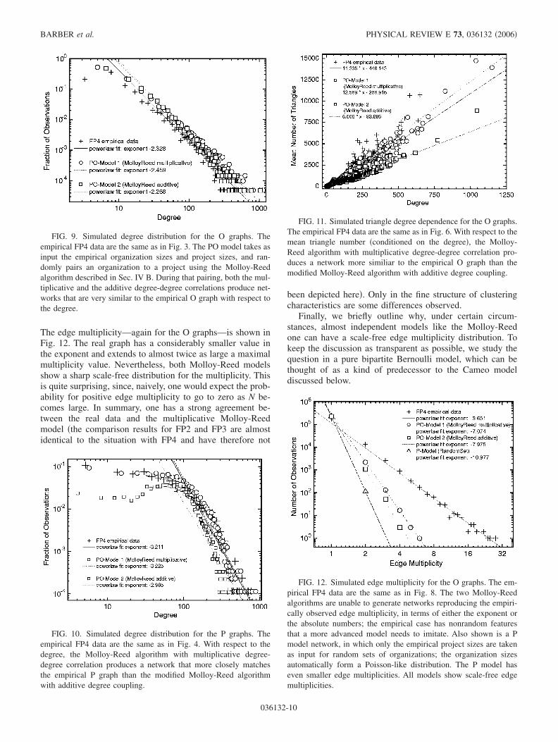
The edge multiplicity—again for the O graphs—is shown inFig. 12. The real graph has a considerably smaller value inthe exponent and extends to almost twice as large a maximalmultiplicity value. Nevertheless, both Molloy-Reed modelsshow a sharp scale-free distribution for the multiplicity. Thisis quite surprising, since, naively, one would expect the prob-ability for positive edge multiplicity to go to zero as N be-comes large. In summary, one has a strong agreement be-tween the real data and the multiplicative Molloy-Reedmodel �the comparison results for FP2 and FP3 are almostidentical to the situation with FP4 and have therefore not

been depicted here�. Only in the fine structure of clusteringcharacteristics are some differences observed.

Finally, we briefly outline why, under certain circum-stances, almost independent models like the Molloy-Reedone can have a scale-free edge multiplicity distribution. Tokeep the discussion as transparent as possible, we study thequestion in a pure bipartite Bernoulli model, which can bethought of as a kind of predecessor to the Cameo modeldiscussed below.

FIG. 9. Simulated degree distribution for the O graphs. Theempirical FP4 data are the same as in Fig. 3. The PO model takes asinput the empirical organization sizes and project sizes, and ran-domly pairs an organization to a project using the Molloy-Reedalgorithm described in Sec. IV B. During that pairing, both the mul-tiplicative and the additive degree-degree correlations produce net-works that are very similar to the empirical O graph with respect tothe degree.

FIG. 10. Simulated degree distribution for the P graphs. Theempirical FP4 data are the same as in Fig. 4. With respect to thedegree, the Molloy-Reed algorithm with multiplicative degree-degree correlation produces a network that more closely matchesthe empirical P graph than the modified Molloy-Reed algorithmwith additive degree coupling.

FIG. 11. Simulated triangle degree dependence for the O graphs.The empirical FP4 data are the same as in Fig. 6. With respect to themean triangle number �conditioned on the degree�, the Molloy-Reed algorithm with multiplicative degree-degree correlation pro-duces a network more similiar to the empirical O graph than themodified Molloy-Reed algorithm with additive degree coupling.

FIG. 12. Simulated edge multiplicity for the O graphs. The em-pirical FP4 data are the same as in Fig. 8. The two Molloy-Reedalgorithms are unable to generate networks reproducing the empiri-cally observed edge multiplicity, in terms of either the exponent orthe absolute numbers; the empirical case has nonrandom featuresthat a more advanced model needs to imitate. Also shown is a Pmodel network, in which only the empirical project sizes are takenas input for random sets of organizations; the organization sizesautomatically form a Poisson-like distribution. The P model haseven smaller edge multiplicities. All models show scale-free edgemultiplicities.


036132-10

To each vertex from the O and P partitions �with cardinal-ity N and M�, we assign a power-law distributed, positiveinteger parameter ��P� and �O� with exponents � and �.That is we partition the P and O vertices into setsD�ª ��P��P�=�� and G ª � �O� �O�= �� such that �D��=

CPM

�� and �G �=CON

� where CP and CO are normalization con-stants. We further assume that M and N are proportional withCop=M /N, and put

Pr�P � O� ªc

N��P� �O� . �21�

In Eq. �21�, c is a free parameter; the ratio c /N regulates thenumber of edges realized in the network. It is easily shownthat the expected degree, conditioned on the � or value, isproportional to � or , respectively, and therefore the �bipar-tite� degree distribution on each partition has the same expo-nent as � or . Note that the maximal � and values aregiven by �max�M1/� and max�N1/�.

Since the edge multiplicity in the projection graph corre-sponds to the number of paths of length 2 in the bipartitegraph, we define Ek

�P2�ªE��P , P��: there are exactly k paths

of length 2 between P and P�� and E�P2�ª�kEk

�P�. For fixedP and P� with parameters � and �� the expected number ofpaths of length 2 between the two vertices is given by

�

c2

N2�� 2�G � �22�

and therefore the expected total number of 2-paths in the Ppartition is

E�P2� = ��,��

�D��D��

c2

N2�� 2�G � �23�

= ��,��

�

COCP2 M

Cop��−1 �−2 . �24�

On the other hand, we have for the probability of an edgebetween P and P� in the P-projection graph the estimate

Pr�P � P�� = 1 − � 1 −

c2

N2�� 2�G �

�25�

�1 − exp− �

COc2��

CopM �−2 �26�

and hence for the expected total number of edges E

E � ��,��

CP2 M2

��1 − exp− �

COc2��

CopM �−2 . �27�

Several cases are now possible. For ��3 and ��2, it iseasy to see that limN→

E�P2�

E =1 and higher edge multiplicitieshave essentially zero probability.

The situation is different if either condition is violated,since in this case E�P2�−E diverges and can become of thesame order as E. For instance, we obtain for ��3,��2

E�P2� − E � ��,��

�max CP2 M2

�� k�2

�− 1�k

k!�

max COc2��

CopM �−2k

�28�

� ��,��

�max const � M2

�� k�2

�− 1�k

k!�const

� ��M3/�−2�k �29�

� �k�2

const ��− 1�k

k!M2/�+k�3/�+2/�−2�. �30�

From the last formula, we see that the expected edge multi-plicity E�P2�

E −1 can become positive for proper choices of �and �. We show that E

E�p2� �1 under the above assumptions.Since

E�P2� = ��,��

�

COCP2 M

Cop��−1 �−2 �31�

�const � M�1/��2�2−��+1+�1/��3−�� 32�

=const � M4/�+3/�−2 �33�

and

E � �k�1

const ��− 1�k+1

k!M2/�+k�3/�+2/�−2�, �34�

one gets

E

E�P2� � 1 − �k�2

const ��− 1�k

k!M2�k−1�/�+3�k−1�/�−2k

�35�

�1 − const � M−2/�−3/��M2/�+3/� − 1 + o�1��36�

=1 − const + o�1� . �37�

Since the involved constant is positive we get the desiredresult. A more careful analysis, which will be part of a forth-coming paper, shows that one also obtains a power law forthe edge multiplicity, as observed in the simulations.

C. Random intersection graphs and the cameo principle

In this section, we give a possible explanation for theappearance of power laws in the size distribution. In mostmodels of complex networks with power-law-like degreedistributions, one assumes a kind of preferential attachmentrule, as in the Albert and Barabási model �3�. This makeslittle sense in our framework. Instead we make use of thecameo principle, first formulated in �8�.

Before giving an interpretation and motivation we brieflydescribe the formal setting. Assign to each project a positive,


036132-11

�-distributed random variable � and to each organization apositive, �-distributed random variable � �note that, in con-trast to Sec. IV B, � and � are not the size distributions�. Weassume � and � to be supported on �1,� and monotonedecreasing as � and � tend to infinity. We also make useof the notational simplifications ��P�=�(��P�) and ��O�=��O��. On the bipartite graph, an edge between an orga-nization O and a project P is then formed with probability

po,p ªc0

��P�1

�P�−��P�

+c1

��O�1

�O�−��O�

, �38�

where c0 and c1 are positive constants, the exponents � and� are in the interval �0,1�, and all edges are drawn indepen-dently of one another. We are interested in the properties ofthe corresponding random P and O graphs for typical real-izations of the � and � variables. The word typical is hereunderstood in the sense of the ergodic theorem, namely, weassume 1

N�O�−��O��1−�d�¬C0−1 and 1

M �P�−��P��1−�d�¬C1

−1, where N and M are the cardinalities of theO and P partitions and � and � are such that the integral isbounded. The above formula reduces then to

po,p ªc0C0

M��P�+

c1C1

N��O�. �39�

The expected conditional size of a vertex is then given by

E��P��P�� =Nc0C0

C1M��P�+ c1 �40�

and

E��O��O�� =Mc1C1

C0N��O�+ c0. �41�

The interpretation behind the special form of edge prob-ability in Eq. �39� is the following. The � and � valuesdescribe a kind of attractivity property inherent to projectsand organizations. Thinking in terms of a virtual project for-mation process either the final set of organizations belongingto a project P can join the project actively—in which casethe � value of P is important—or the organization morepassively enters the project on the request of organizationsalready involved—in which case the attractivity � of the thecorresponding organization is important. The attractivity ofan organization could, for instance, be related to its reputa-tion, financial strength, or quality of earlier projects in whichthe organization was involved. The pairing probability is notdirectly based on the � or � values, but rather the relativefrequency of the � or � values: the rarer a property, the moreattractive it becomes. This is the essence of the cameo prin-ciple.

The parameters � and � can be seen as defining the pro-pensity to follow the above rule; for � ,�→0 the rule isswitched off and we recover a classical Erdös-Renyi inter-section graph. In general the values of � and � are them-selves quenched random variables with their own—usuallyunknown—distribution. As shown in �12�, only the maximal

� and � values matter for the resulting degree distribution ofthe graphs. We therefore restrict ourselves in the following toconstant values.

Since the conditional expectations of the size values �Eqs.�40� and �41�� are proportional to �−� and �−�, we have toestimate their induced distribution. It can be shown �13� thatzª�−�� is asymptotically distributed with densityz−�1+1/�+o�1�� when �� decays monotonically and faster thanany power law to zero as �→. When �� is itself apower-law distribution with exponent �, the resulting distri-bution for z will be z−�1+1/�−1/��+o�1��. Therefore, the induceddistribution is always a power law and independent of thedetails of �. Applying this result to our model, we obtainimmediately a power-law distribution for the size distribu-tion on the P and O graphs with exponents depending essen-tially only on � and �. Due to the edge independence in themodel definition, the resulting degree distributions are againof power-law type. The cameo ansatz hence generates in anatural way a bipartite graph, where both projections admittwo of the main features of the FP networks. Furthermore,we obtain a linear dependence of the mean triangle number�k on the degree, as in Sec. IV A.

None of the models discussed in Sec. IV can reproducescale-free distribution of the edge multiplicity with the samelow exponent as observed in each of the FP networks. It willbe interesting to see whether the inclusion of memory effectslike the “my friends are your friends” principle �14� willchange the picture.

V. CONCLUSIONS

In this paper, we have described research collaborationnetworks determined from research projects funded by theEuropean Union. The networks are substantial in terms ofsize, complexity, and economic impact. We observed numer-ous characteristics known from other complex networks, in-cluding scale-free degree distribution, small diameter, andhigh clustering. Using a random intersection-graph model,we were able to reproduce many properties of the actualnetworks. The empirical and theoretical investigations to-gether shed light on the properties of these complex net-works, in particular that the EU-funded research and devel-opment networks match well with typical realizations ofrandom graph models characterized by just four parameters:the size, edge number, exponent of project-projection degreedistribution, and exponent of organization-projection degreedistribution.

In terms of real-world interpretation, the present analysisyields three major insights. First, based on the fact that thesize distribution of projects did not change significantly be-tween the Framework Programs, any possible changes inproject formation rules—which we do not know at thisstage—did not affect the aggregate structure of the resultingresearch networks. Second, the fact that integration betweencollaborating organizations has increased over time, as mea-sured by the average clustering coefficient, indicates that Eu-rope has already been moving toward a more closely inte-grated European Research Area in the earlier FrameworkPrograms. Finally, the fact that a sizable number of organi-


036132-12

zations collaborate more than once in each Framework Pro-gram shows that there appears to be a kind of robust back-bone structure in place, which may constitute the core of theEuropean Research Area.

In terms of application, the present results suggest a num-ber of extensions. First, it is essential to learn more about theproperties of the vertices in our networks. To what extent canthey be characterized and classified? What kind of structuralpatterns emerge if we add this information? Second, we needto know more about the microstructure of the networks. Inwhich areas are the networks highly clustered and wheredoes this clustering come from? What kind of subgroups canbe identified? Third, we need to learn more about where theobserved distribution of edge multiplicity comes from. Fi-nally, it would be desirable to explicitly include edge weightsinto the analysis, as actors who collaborate frequently arepresumably more proximate to each other than actors who

collaborate only once. This may significantly impact thestructural features we are able to observe, as well as theconclusions we might draw concerning the link between net-work structure and function.

ACKNOWLEDGMENTS

We would like to acknowledge support from the Portu-guese Fundação para a Ciência e a Tecnologia �Bolsa deInvestigação SFRH/BPD/9417/2002 and FEDER/POCTI-SFA-1-219�, ARC systems research �W4570000294-3�, andthe VW Stiftung �I/80496�. We thank Ph. Blanchard and L.Streit for useful discussions and commentary. Portions of thiswork were done at the Vienna Thematic Institute for Com-plexity and Innovation, EXYSTENCE Network of Excel-lence: IST-2001-32802.

�1� D. J. Watts and S. H. Strogatz, Nature �London� 393, 440�1998�.

�2� B. Bollobás and J. Riordan, in Handbook of Graphs and Net-works �Wiley-VCH, Berlin, 2003�.

�3� R. Albert and A.-L. Barabási, Rev. Mod. Phys. 74, 47 �2002�.�4� M. Karonski, E. R. Scheinerman, and K. B. Singer-Cohen,

Combinatorics, Probab. Comput. 8, 131 �1999�.�5� K. Barker and H. Cameron, in European Collaboration in Re-

search and Development, edited by Y. Caloghirou, N. S.Vonortas, and S. Ioannides �Edward Elgar, Cheltenham, U.K.,2004�.

�6� CORDIS Projects Database—Advanced and Professional Da-tabase Search, http://dbs.cordis.lu/cordis-cgi/EI&CALLER�EIPROF_EN_PROJ&MODE�N&LANGUAGE�EN&DATABASE�PROJ.

�7� M. E. J. Newman, Phys. Rev. E 64, 016131 �2001�.�8� Ph. Blanchard and T. Krueger, J. Stat. Phys. 114, 5 �2004�.�9� M. Molloy and B. Reed, Random Struct. Algorithms 6,

161180 �1995�.�10� B. Bollobás, Eur. J. Comb. 1, 311316 �1980�.�11� Ph. Blanchard, A. Krüger, T. Krueger, and P. Martin, e-print

physics/0505031.�12� Ph. Blanchard, S. Fortunato, and T. Krueger, Phys. Rev. E 71,

056114 �2005�.�13� Ph. Blanchard and T. Krueger, in Extreme Events in Nature

and Society, The Frontier Collections �Springer, Berlin, 2006�.�14� Ph. Blanchard, T. Krueger, and A. Ruschhaupt, Phys. Rev. E

71, 046139 �2005�.


036132-13