NBER WORKING PAPER SERIES
EMPIRICAL EXCHANGE RATE MODELSOF THE NINETIES:
ARE ANY FIT TO SURVIVE?
Yin-Wong CheungMenzie D. Chinn
Antonio Garcia Pascual
Working Paper 9393http://www.nber.org/papers/w9393
NATIONAL BUREAU OF ECONOMIC RESEARCH1050 Massachusetts Avenue
Cambridge, MA 02138December 2002
We thank, without implicating, Jeff Frankel, Fabio Ghironi, Jan Groen, Lutz Kilian, Ed Leamer, RonaldMacDonald, David Papell, John Rogers, Lucio Sarno, Torsten Sløk, Frank Westermann, seminar participantsat Academica Sinica, Boston College, UCLA, University of Houston and conference participants at CES-ifoVenice Summer Institute conference on “Exchange Rate Modeling” for helpful comments, and JeannineBailliu, Gabriele Galati and Guy Meredith for providing data. The financial support of faculty research fundsof the University of California, Santa Cruz is gratefully acknowledged. The views expressed herein are thoseof the authors and not necessarily those of the International Monetary Fund or the National Bureau ofEconomic Research.
© 2002 by Yin-Wong Cheung, Menzie D. Chinn, and Antonio Garcia Pascual. All rights reserved. Shortsections of text not to exceed two paragraphs, may be quoted without explicit permission provided that fullcredit including, © notice, is given to the source.

Empirical Exchange Rate Models of the Nineties:Are Any Fit to Survive?Yin-Wong Cheung, Menzie D. Chinn, and Antonio Garcia PascualNBER Working Paper No. 9393December 2002JEL No. F31, F47
ABSTRACT
Previous assessments of nominal exchange rate determination have focused upon a narrowset of models typically of the 1970’s vintage. The canonical papers in this literature are by Meeseand Rogoff (1983, 1988), who examined monetary and portfolio balance models. Succeeding worksby Mark (1995) and Chinn and Meese (1995) focused on similar models. In this paper we re-assessexchange rate prediction using a wider set of models that have been proposed in the last decade:interest rate parity, productivity based models, and "behavioral equilibrium exchange rate" models.The performance of these models is compared against a benchmark model – the Dornbusch-Frankelsticky price monetary model. The models are estimated in error correction and first-differencespecifications. Rather than estimating the cointegrating vector over the entire sample and treatingit as part of the ex ante information set as is commonly done in the literature, we recursively updatethe cointegrating vector, thereby generating true ex ante forecasts. We examine model performanceat various forecast horizons (1 quarter, 4 quarters, 20 quarters) using differing metrics (mean squarederror, direction of change), as well as the Aconsistency@ test of Cheung and Chinn (1998). No modelconsistently outperforms a random walk, by a mean squared error measure; however, along adirection-of-change dimension, certain structural models do outperform a random walk withstatistical significance. Moreover, one finds that these forecasts are cointegrated with the actualvalues of exchange rates, although in a large number of cases, the elasticity of the forecasts withrespect to the actual values is different from unity. Overall, model/specification/currencycombinations that work well in one period will not necessarily work well in another period.
Yin-Wong Cheung Menzie D. Chinn Antonio Garcia PascualDepartment of Economics Department of Economics International Monetary FundUniversity of California University of California 700 19th Street, NWSanta Cruz, CA 95064 Santa Cruz, CA 95064 Washington, DC [email protected] and NBER [email protected]

1
1. Introduction
The recent movements in the dollar and the euro have appeared seemingly inexplicable in
the context of standard models. While the dollar may not have been Adazzling@ – as it was
described in the mid-1980's – it has been characterized as overly Adarling.@1 And the euro=s
ability to repeatedly confound predictions needs little re-emphasizing.
It is against this backdrop that several new models have been forwarded in the past
decade. Some explanations are motivated by new findings in the empirical literature, such the
correlation between net foreign asset positions and real exchange rates. Others, such as those
based on productivity differences, are solidly grounded in the theoretical literature. None of
these models, however, have been subjected to rigorous examination of the sort that Meese and
Rogoff conducted in their seminal work, the original title of which we have appropriated and
amended for this study.2
We believe that a systematic examination of these newer empirical models is long
overdue, for a number of reasons. First, while these models have become prominent in policy
and financial circles, they have not been subjected to the sort of rigorous out-of-sample testing
conducted in academic studies. For instance, behavioral equilibrium exchange rate models –
essentially combinations of real interest differential, productivity and portfolio balance models –
have been used in estimating the “equilibrium” values of the dollar and the euro.3
Second, most of the recent academic treatments exchange rate forecasting performance
rely upon a single model – such as the monetary model – or some other limited set of models of
1970’s vintage. Thus, in the recent Journal of International Economics symposium celebrating
the 20th anniversary of the Meese-Rogoff papers, the nominal exchange rate approaches applied
1 Frankel (1985) and The Economist (2001), respectively.
2 Meese and Rogoff (1983) was based upon work in “Empirical exchange rate models of the seventies: are any fit to survive?” International Finance Discussion Paper No. 184 (Board of Governors of the Federal Reserve System, 1981).
3 For the euro: Morgan Stanley (Fels and Yilmaz, 2001), Bundesbank (Clostermann and Schnatz, 2000), ECB ( Maeso-Fernandez et al., 2001), and IMF (Alberola, et al., 1999). For the dollar: Morgan Stanley (Yilmaz and Jen, 2001).
2
to the G-3 currencies included the flexible price monetary model, purchasing power parity, and
the interest differential.
Third, the same criteria are often used, neglecting many alternative dimensions of model
forecast performance. That is, the first and second moment metrics such as mean error and mean
squared error are considered, while other aspects that might be of greater importance are often
neglected. We have in mind the direction of change – perhaps more important from a market
timing perspective – and other indicators of forecast attributes.
In this study, we extend the forecast comparison of exchange rate models in several
dimensions.
• Four models are compared against the random walk. Only one of the structural models – the
benchmark sticky-price monetary model of Dornbusch and Frankel – has been the subject of
previous systematic analyses. The other models include one incorporating productivity
differentials in a fashion consistent with a Balassa-Samuelson formulation, an interest rate
parity specification, and a representative behavioral equilibrium exchange rate model.
• The behavior of US dollar-based exchange rates of the Canadian dollar, British pound,
Deutsche mark and Japanese yen are examined. We also examine the corresponding yen-
based rates, to insure that our conclusions are not driven by dollar specific results.
• The models are estimated in two ways: in first-difference and error correction specifications.
• Forecasting performance is evaluated at several horizons (1-, 4- and 20-quarter horizons) and
two sample periods (post-Louvre Accord and post-1982).
• We augment the conventional metrics with a direction of change statistic and the
“consistency” criterion of Cheung and Chinn (1998).
In accord with previous studies, we find that no model consistently outperforms a random
walk according to the mean squared error criterion at short horizons. Somewhat at variance with
some previous findings, we find that the proportion of times the structural models incorporating
long-run relationships outperform a random walk at long horizons is slightly less than would be
expected if the outcomes were merely random.
On the other hand, the direction-of-change statistics indicate that the structural models do
outperform a random walk characterization by a statistically significant amount. For instance,

3
using a 10% significance level, the sticky price model outperforms a random walk 23% of the
time for dollar-based exchange rates. For yen based exchange rates, the interest rate parity model
outperforms a random walk 37% of the time.
In terms of the “consistency” test of Cheung and Chinn (1998), similarly positive results
are obtained. The actual and forecasted rates are cointegrated more often than would occur by
chance for all the models. While in many of these cases of cointegration, the condition of unitary
elasticity of expectations is rejected, between 12% to 13% fulfill all the conditions of the
consistency criteria.
We conclude that the question of exchange rate predictability remains unresolved. In
particular, while the oft-used mean squared error criterion provides a dismal perspective, criteria
other than the conventional ones suggest that structural exchange rate models have some
usefulness. Furthermore, the best model and specification tend to be specific to the currency and
out-of-sample forecasting period.
2. Theoretical Models
The universe of empirical models that have been examined over the floating rate period is
enormous. Consequently any evaluation of these models must necessarily be selective. Our
criteria require that the models are (1) prominent in the economic and policy literature, (2)
readily implementable and replicable, and (3) not previously evaluated in a systematic fashion.
We use the random walk model as our benchmark naive model, in line with previous work, but
we also select one workhorse model, the basic Dornbusch (1976) and Frankel (1979) model as a
comparator specification, as it still provides the fundamental intuition for how flexible exchange
rates behave. The sticky price monetary model can be expressed as follows:
(1) ,ˆˆˆˆ tt4t3t2t10t u + i + y + m + = s +πβββββ
where m is log money, y is log real GDP, i and π are the interest and inflation rate, respectively,
A^@ denotes the intercountry difference, and ut is an error term.
The characteristics of this model are well known, so we will not devote time to
discussing the theory behind the equation. We will observe, however, that the list of variables
included in (1) encompasses those employed in the flexible price version of the monetary model,
4
as well as the micro-based general equilibrium models of Stockman (1980) and Lucas (1982).
Second, we assess models that are in the Balassa-Samuelson vein, in that they accord a
central role to productivity differentials to explaining movements in real, and hence also
nominal, exchange rates. Real versions of the model can be traced to DeGregorio and Wolf
(1994), while nominal versions include Clements and Frenkel (1980) and Chinn (1997). Such
models drop the purchasing power parity assumption for broad price indices, and allow the real
exchange rate to depend upon the relative price of nontradables, itself a function of productivity
(z) differentials. A generic productivity differential exchange rate equation is
(2) tt53210t uz + i + y + m + = s +ˆˆˆˆ βββββ .
The third set of models we examine includes the behavioral equilibrium exchange rate
models. This is a diverse set of models that incorporate a number of familiar and unfamiliar
relationships. A typical specification is:
(3) ,ˆˆˆˆ tt9t8t7t6t5t0t unfa + tot + debtg + r + + p + = s +ββββωββ
where p is the log price level (CPI), ω is the relative price of nontradables, r is the real interest
rate, gdebt the government debt to GDP ratio, tot the log terms of trade, and nfa is the net foreign
asset. This specification can be thought of as incorporating the Balassa-Samuelson effect, the
real interest differential model, an exchange risk premium associated with government debt
stocks, and additional portfolio balance effects arising from the net foreign asset position of the
economy.4 Clark and MacDonald (1999) is a recent exposition of this approach.
Models based upon this framework have been the predominant approach to determining
the rate at which currencies will gravitate to over some intermediate horizon, especially in the
context of policy issues. For instance, the behavioral equilibrium exchange rate approach is the
model that is most used to determine the long-term value of the euro.5
4 On this latter channel, Cavallo and Ghironi (2002) provide a role for net foreign assets
in the determination of exchange rates in the sticky-price optimizing framework of Obstfeld and Rogoff (1995).
5 We do not examine two closely related approaches: the internal-external balance approach of the IMF (see Faruqee, Isard and Masson, 1999) and the NATREX approach (Stein, 1999). The IMF approach requires extensive judgements regarding the trend level of output, and the impact of demographic variables upon various macroeconomic aggregates. We did not

5
The final specification assessed is not a model per se; rather it is an arbitrage relationship
– uncovered interest rate parity:
(4) s s it k t t k+ = + $ ,
where it,k is the interest rate of maturity k. Unlike the other specifications, this relation need not
be estimated in order to generate predictions.
Interest rate parity at long horizons has recently gathered empirical support (Alexius,
2001 and Meredith and Chinn, 1998), in contrast to the disappointing results at the shorter
horizons. MacDonald and Nagayasu (2000) have also demonstrated that long-run interest rates
appear to predict exchange rate levels. On the basis of these findings, we anticipate that this
specification will perform better at the longer horizons than at shorter.6
3. Data, Estimation and Forecasting Comparison
3.1 Data
The analysis uses quarterly data for the United States, Canada, UK, Japan, Germany, and
Switzerland over the 1973q2 to 2000q4 period. The exchange rate, money, price and income
variables are drawn primarily from the IMF’s International Financial Statistics. The productivity
data were obtained from the Bank for International Settlements, while the interest rates used to
conduct the interest rate parity forecasts are essentially the same as those used in Meredith and
Chinn (1998)). See the Data Appendix for a more detailed description.
Two out-of-sample periods are used to assess model performance: 1987q2-2000q4 and
1983q1-2000q4. The former period conforms to the post-Louvre Accord period, while the latter
spans the period after the end of monetary targeting in the U.S. Figures 1 and 2 depict,
respectively, the dollar based Deutschemark and yen exchange rates, with the right-most line
believe it would be possible to subject this methodology to the same out of sample forecasting exercise applied to the others. The NATREX approach is conceptually different from the BEER methodology. However, it shares a sufficiently large number of attributes with the latter that we decided not to separately examine it.
6 Despite this finding, there is little evidence that long term interest rate differentials – or equivalently long-dated forward rates – have been used for forecasting at the horizons we are investigating. One exception from the non-academic literature is Rosenberg (2001).
6
indicating the beginning of the first out-of-sample period, and the left-most line indicating the
second. The shorter out-of-sample period (1987-2000) spans a period of relative dollar stability
(and appreciation in the case of the mark). The longer out-of-sample period subjects the models
to a more rigorous test, in that the prediction takes place over a large dollar appreciation and
subsequent depreciation (against the mark) and a large dollar depreciation (from 250 to 150 yen
per dollar). In other words, this longer span encompasses more than one “dollar cycle.” The use
of this long out-of-sample forecasting period has the added advantage that it ensures that there
are many forecast observations to conduct inference upon. 7
3.2 Estimation and Forecasting
We adopt the convention in the empirical exchange rate modeling literature of
implementing “rolling regressions.” That is, estimates are applied over a given data sample, out-
of-sample forecasts produced, then the sample is moved up, or “rolled” forward one observation
before the procedure is repeated. This process continues until all the out-of-sample observations
are exhausted. This procedure is selected over recursive estimation because it is more in line
with previous work, including the original Meese and Rogoff paper. Moreover, the power of the
test is kept constant as the sample size over which estimation occurs is fixed, rather than
increasing as it does in the recursive framework.
Two specifications of these theoretical models were estimated: (1) an error correction
specification, and (2) a first differences specification. Since implementation of the error
correction specification is relatively involved, we will address the first-difference specification
to begin with. Consider the general expression for the relationship between the exchange rate
and fundamentals:
(5) ttt uX = s +Γ ,
7 We are aware of the debate over the use of out of sample versus in sample tests. Out of
sample tests have been favored as a means of guarding against data mining. Inoue and Kilian (2002) argue that in sample tests often have higher power than out of sample, even after accounting for the effects of data mining. We retain the use of out of sample testing in order to make our findings comparable to those in the literature, and to hew to the tradition of the original Meese-Rogoff papers.

7
where Xt is a vector of fundamental variables under consideration. The first-difference
specification involves the following regression:
(6) ttt uX = s +Γ∆∆ .
These estimates are then used to generate one- and multi-quarter ahead forecasts. Since these
exchange rate models imply joint determination of all variables in the equations, it makes sense
to apply instrumental variables. However, previous experience indicates that the gains in
consistency are far outweighed by the loss in efficiency, in terms of prediction (Chinn and
Meese, 1995). Hence, we rely solely on OLS.
The error correction estimation involves a two step procedure. In the first step, the long-
run cointegrating relation implied by (5) is identified using the Johansen procedure. The
estimated cointegrating vector (~Γ ) is incorporated into the error correction term, and the
resulting equation
(7) tktktktt uXs = ss +Γ−+− −−− )(~
10 δδ
is estimated via OLS. Equation (7) can be thought of as an error correction model stripped of
short run dynamics. A similar approach was used in Mark (1995) and Chinn and Meese (1995),
except for the fact that in those two cases, the cointegrating vector was imposed a priori.
One key difference between our implementation of the error correction specification and
that undertaken in some other studies involves the treatment of the cointegrating vector. In some
other prominent studies (MacDonald and Taylor, 1993), the cointegrating relationship is
estimated over the entire sample, and then out of sample forecasting undertaken, where the short
run dynamics are treated as time varying but the long-run relationship is not. While there are
good reasons for adopting this approach – in particular one wants to use as much information as
possible to obtain estimates of the cointegrating relationships – the asymmetry in estimation
approach is troublesome, and makes it difficult to distinguish quasi-ex ante forecasts from true
ex ante forecasts. Consequently, our estimates of the long-run cointegrating relationship vary as
the data window moves.
It is also useful to stress the difference between the error correction specification
forecasts and the first-difference specification forecasts. In the latter, ex post values of the right

8
hand side variables are used to generate the predicted exchange rate change. In the former,
contemporaneous values of the right hand side variables are not necessary, and the error
correction predictions are true ex ante forecasts. Hence, we are affording the first-difference
specifications a tremendous informational advantage in forecasting.8
3.3 Forecast Comparison
To evaluate the forecasting accuracy of the different structural models, the ratio between
the mean squared error (MSE) of the structural models and a driftless random walk is used. 9A
value smaller (larger) than one indicates a better performance of the structural model (random
walk). We also explicitly test the null hypothesis of no difference in the accuracy of the two
competing forecasts (i.e. structural model vs. driftless random walk). In particular, we use the
Diebold-Mariano statistic (Diebold and Mariano, 1995) which is defined as the ratio between the
sample mean loss differential and an estimate of its standard error; this ratio is asymptotically
distributed as a standard normal. 10 The loss differential is defined as the difference between the
squared forecast error of the structural models and that of the random walk. A consistent
estimate of the standard deviation can be constructed from a weighted sum of the available
8 We opted to exclude short-run dynamics in equation (7) because a) the use of equation
(7) yields true ex ante forecasts and makes our exercise directly comparable with, for example, Mark (1995), Chinn and Meese (1995) and Groen (2000), and b) the inclusion of short-run dynamics creates additional demands on the generation of the right-hand-side variables and the stability of the short-run dynamics that complicate the forecast comparison exercise beyond a manageable level.
9 The comparison could also be made against a random walk with estimated drift, as
suggested by Kilian (1999). We opted not to make this comparison for two reasons. First, over the long samples we are examining, the drift term would be approximately zero (except perhaps for the yen). Second, it is typically easier to outperform a random walk with drift benchmark; hence, in selecting this reference model, we are being conservative by biasing our results against finding structural model performance.
10 In using the DM test, we are relying upon asymptotic results, which may or may not be appropriate for our sample. However, generating finite sample critical values for the large number of cases we deal with would be computationally infeasible. More importantly, the most likely outcome of such an exercise would be to make detection of statistically significant outperformance even more rare, and leaving our basic conclusion intact.
9
sample autocovariances of the loss differential vector. Following Andrews (1991), a quadratic
spectral kernel is employed, together with a data-dependent bandwidth selection procedure.11
We also examine the predictive power of the various models along different dimensions.
One might be tempted to conclude that we are merely changing the well-established “rules of the
game” by doing so. However, there are very good reasons to use other evaluation criteria. First,
there is the intuitively appealing rationale that minimizing the mean squared error (or relatedly
mean absolute error) may not be important from an economic standpoint. A less pedestrian
motivation is that the typical mean squared error criterion may miss out on important aspects of
predictions, especially at long horizons. Christoffersen and Diebold (1998) point out that the
standard mean squared error criterion indicates no improvement of predictions that take into
account cointegrating relationships vis à vis univariate predictions. But surely, any reasonable
criteria would put some weight the tendency for predictions from cointegrated systems to “hang
together”. Hence, our first alternative evaluation metric for the relative forecast performance of the
structural models is the direction of change statistic, which is computed as the number of correct
predictions of the direction of change over the total number of predictions. A value above
(below) 50 per cent indicates a better (worse) forecasting performance than a naive model that
predicts the exchange rate has an equal chance to go up or down. Again, Diebold and Mariano
(1995) provide a test statistic for the null of no forecasting performance of the structural model.
The statistic follows a binomial distribution, and its studentized version is asymptotically
distributed as a standard normal. Not only does the direction of change statistic constitute an
alternative metric, it is also an approximate measure of profitability. We have in mind here tests
for market timing ability (Cumby and Modest, 1987). 12
The third metric we used to evaluate forecast performance is the consistency criterion
11 We also experienced with the Bartlett kernel and the deterministic bandwidth selection
method. The results from these methods are qualitatively very similar. Appendix 2 contains a more detailed discussion of the forecast comparison tests.
12 See also Leitch and Tanner (1991), who argue that a direction of change criterion may
be more relevant for profitability and economic concerns, and hence a more appropriate metric than others based on purely statistical motivations.

10
proposed in Cheung and Chinn (1998). This metric focuses on the time-series properties of the
forecast. The forecast of a given spot exchange rate is labeled as consistent if (1) the two series
have the same order of integration, (2) they are cointegrated, and (3) the cointegration vector
satisfies the unitary elasticity of expectations condition. Loosely speaking, a forecast is
consistent if it moves in tandem with the spot exchange rate in the long run. Cheung and Chinn
(1998) provide a more detailed discussion on the consistency criterion and its implementation.
4. Comparing the Forecast Performance
4.1 The MSE Criterion
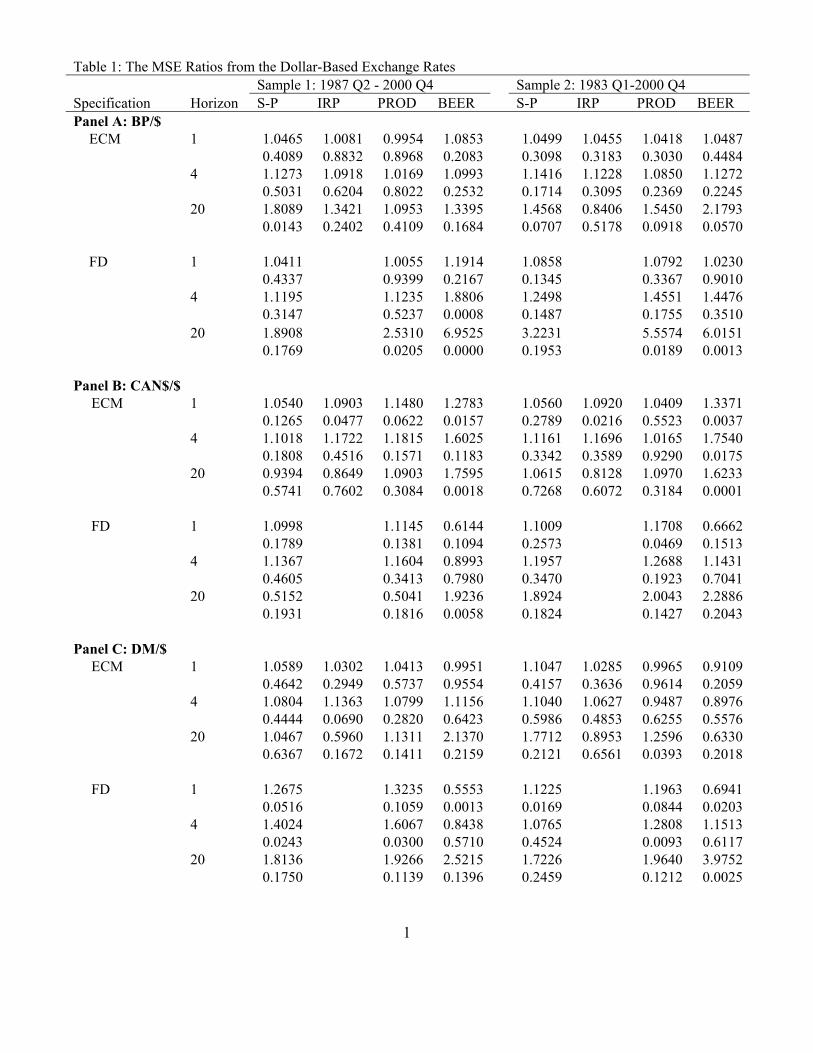
The comparison of forecasting performance based on MSE ratios is summarized in Table
1. The Table contains MSE ratios and the p-values from five dollar-based currency pairs, four
structural models, the error correction and first-difference specifications, three forecasting
horizons, and two forecasting samples. Each cell in the Table has two entries. The first one is the
MSE ratio (the MSEs of a structural model to the random walk specification). The entry
underneath the MSE ratio is the p-value of the hypothesis that the MSEs of the structural and
random walk models are the same. Because of the lack of data, the behavioral equilibrium
exchange rate model is not estimated for the dollar-Swiss franc and dollar-yen exchange rates.
Altogether, there are 186 MSE ratios, which spread evenly across the two forecasting samples.
Of these 186 ratios, 108 are computed from the error correction specification and 78 from the
first-difference one.
Note that in the tables, only “error correction specification” entries are reported for the
interest rate parity model. In fact, this model is not estimated; rather the predicted spot rate is
calculated using the uncovered interest parity condition. To the extent that long term interest
rates can be considered the error correction term, we believe this categorization is most
appropriate.
Overall, the MSE results are not favorable to the structural models. Of the 186 MSE
ratios, 141 are not significant (at the 10% significance level) and 45 are significant. That is, for
the majority cases one cannot differentiate the forecasting performance between a structural
model and a random walk model. For the 45 significant cases, there are 43 cases in which the

11
random walk model is significantly better than the competing structural models and only 2 cases
in which the opposite is true. The significant cases are quite evenly distributed across the two
forecasting periods. As 10% is the size of the test and 3 cases constitute less than 10% of the
total of 186 cases, the empirical evidence can hardly be interpreted as supportive of the superior
forecasting performance of the structural models.
Inspection of the MSE ratios, does not reveal many consistent patterns in terms of
outperformance. It appears that the productivity model does not do particularly badly for the
dollar-mark rate at the 1- and 4-quarter horizons. The MSE ratios of the interest rate parity
model are less than unity only at the 20-quarter horizon – a finding consistent with the well-
known bias in forward rates at short horizons.
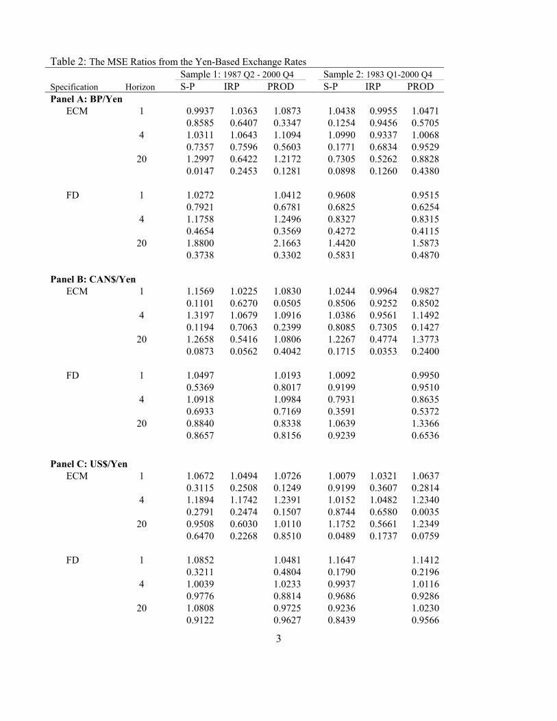
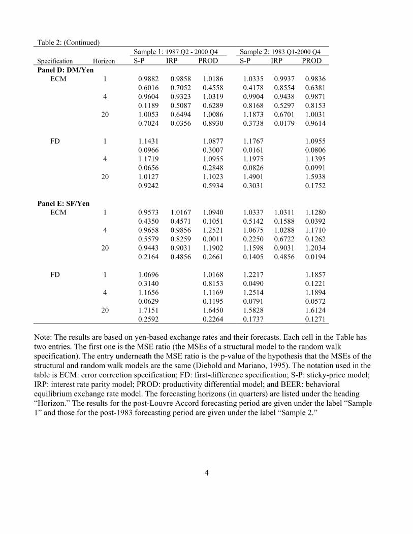
The MSE results derived from the yen-based exchange rates are provided in Table 2,
which has a format similar to that of Table 1. As we lack data to estimate the behavioral
equilibrium exchange rate model for yen-based exchange rates, Table 2 contains only 150 MSE
ratios and the p-values of the hypothesis that the MSEs of the structural and random walk models
are the same. Again, the structural models do not deliver a better forecasting performance than a
random walk model. Indeed, compared with the dollar-based exchange rates, the yen-based
exchange rates have a larger fraction of cases in which one cannot differentiate the forecasting
performance between a structural model and a random walk model. In 126 out of 150 cases, the
statistic is not significant. Of the significant cases, the random walk model outperforms in 20
cases and the competing structural models do better in 4 cases. Again, the frequency of
observing a structural model forecast better than a random walk model is lower than that implied
by the size of the test.
Consistent with the existing literature, our results are supportive of the assertion that it is
very difficult to find forecasts from a structural model that can consistently beat the random walk
model using the MSE criterion. The current exercise further strengthens the assertion as it covers
both dollar- and yen-based exchange rates, two different forecasting periods, and some structural
models that have not been extensively studied before.

12
4.2 The Direction of Change Criterion
Table 3 reports the proportion of forecasts that correctly predict the direction of the dollar
exchange rate movement and, underneath these sample proportions, the p-values for the
hypothesis that the reported proportion is significantly different from ½. When the proportion
statistic is significantly larger than ½, the forecast is said to have the ability to predict the direct
of change. On the other hand, if the statistic is significantly less than ½, the forecast tends to give
the wrong direction of change. For trading purposes, information regarding the significance of
incorrect prediction can be used to derive a potentially profitable trading rule by going again the
prediction generated by the model. Following this argument, one might consider the cases in
which the proportion of "correct" forecasts is larger than or less than ½ contain the same
information. However, in evaluating the ability of the model to describe exchange rate behavior,
we separate the two cases.
There is mixed evidence on the ability of the structural models to correctly predict the
direction of change. Among the 186 direction of change statistics, 32 (22) are significantly larger
(less) than ½ at the 10% level. The occurrence of the significant outperformance cases is higher
(17%) than the one implied by the 10% level of the test. The results indicate that the structural
model forecasts can correctly predict the direction of the change, while the proportion of cases
where a random walk outperforms the competing models is only about what one would expect if
they occurred randomly.
Let us take a closer look at the incidences in which the forecasts are in the right direction.
Approximately 1/3 of the 32 cases are associated with the error correction model and the
remainder with the first difference specification. Thus, it is not clear if the error correction
specification – which incorporates the empirical long-run relationship – is a better specification
for the models under consideration. The forecasting period does not have a major impact on
forecasting performance, since exactly half of the successful cases are in each forecasting period.
Among the four models under consideration, the sticky-price model has the highest
number (10) of forecasts that give the correct direction of change prediction, closely followed by
the behavioral equilibrium exchange rate and productivity models (9 and 8 respectively), and the
13
interest rate parity model (5). Thus, at least on this count, the newer exchange rate models do not
edge out the “old fashioned” sticky-price model. Because there are differing numbers of
forecasts due to data limitations and specifications, the proportions do not exactly match up with
the numbers. Proportionately, the behavioral equilibrium exchange rate model does the best.
Interestingly, the success of direction of change prediction appears to be currency
specific. The dollar-yen exchange rate yields 9 out of 30 forecasts that give the correct direction
of change prediction. In contrast, the dollar-pound has only 2 out of 42 forecasts that produce the
correct direction of change prediction.
The cases of correct direction prediction appear to cluster at the long forecast horizon.
The 20-quarter horizon accounts for 14 of the 32 cases while the 4-quarter and 1-quarter
horizons have 10 and 8 direction of change statistics that are significantly larger than ½. Since
there have not been many studies utilizing the direction of change statistic in similar contexts, it
is difficult to make comparisons. Chinn and Meese (1995) apply the direction of change statistic
to 3 year horizons for three conventional models, and find that performance is largely currency-
specific: the no change prediction is outperformed in the case of the dollar-yen exchange rate,
while all models are outperformed in the case of the dollar-pound rate. In contrast, in our study
at the 20-quarter horizon, the positive results appear to be fairly evenly distributed across the
currencies, with the exception of the dollar-pound rate.13 Mirroring the MSE results, it is
interesting to note that the direction of change statistic works for the interest rate parity model
only at the 20-quarter horizon. This pattern is entirely consistent with the finding that uncovered
interest parity holds better at long horizons. 14
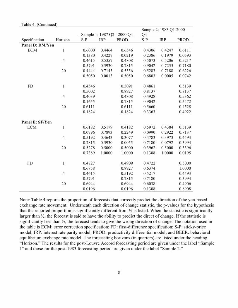
The direction of change results derived from the yen-based exchange rates are
summarized in Table 4. Of the 150 yen-based direction of change statistics, 37 (or 25%) are
significantly larger than ½ while 7 are significantly smaller. The 37 cases in which the forecasts
13 Using Markov switching models, Engel (1994) obtains some success along the
direction of change dimension at horizons of up to one year. However, his results are not statistically significant.
14 Mark and Moh (2001) document the gradual currency appreciation in response to a short term interest differential, contrary to the predictions of uncovered interest parity.
14
give correct direction of change predictions distribute evenly across the three models (sticky
price, interest rate parity, and productivity differential) under consideration, although on a
proportional basis the interest rate parity model garners the highest success ratio (37%). Similar
to the dollar based data, the direction of change results appear to be currency specific and the
outperformance is concentrated in the pound-yen exchange rate. Among the 37 cases in which
the structure models correctly predict the direction of change, the 20-quarter ahead forecast
horizon accounts for 20 cases while the 1-quarter and 4-quarter ahead forecast horizons have 5
and 12 cases respectively. The direction of change outperformance is more pronounced at the
long horizon. This is in line with the results of Mark (1995) and Chinn and Meese (1995).
4.3 The Consistency Criterion
The consistency criterion only requires the forecast and actual realization comove one-to-
one in the long run. One may argue that the criterion is less demanding than the MSE and direct
of change metrics. Indeed, a forecast that satisfies the consistency criterion can (1) have a MSE
larger than that of the random walk model, (2) have a direction of change statistic less than ½, or
(3) generate forecast errors that are serially correlated. However, given the problems related to
modeling, estimation, and data quality, the consistency criterion can be a more flexible way to
evaluate a forecast. In assessing the consistency, we first test if the forecast and the realization
are cointegrated.15 If they are cointegrated, then we test if the cointegrating vector satisfies the
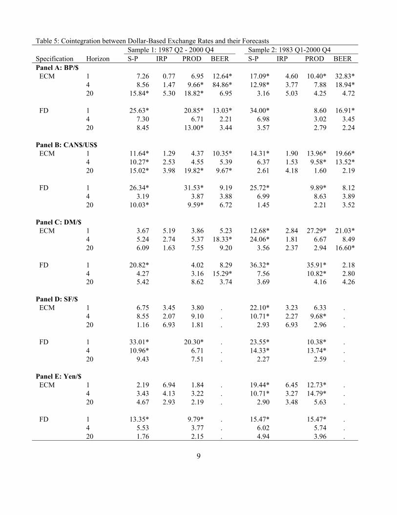
(1, -1) requirement. The cointegration results are reported in Tables 5 and 6. The test results for
the (1, -1) restriction are reported in Tables 7 and 8.
For the dollar-based exchange rate data, 62 of 186 cases reject the null hypothesis of no
cointegration at the 10% significance level. Thus, 62 forecast series (33% of the total number)
are cointegrated with the corresponding spot exchange rates. The error correction specification
accounts for 34 of the 62 cointegrated cases and the first-difference specification accounts for the
15 The Johansen method is used to test the null hypothesis of no cointegration. The
maximum eigenvalue statistics are reported in the manuscript. Results based on the trace statistics are essentially the same. Before implementing the cointegration test, both the forecast and exchange rate series were checked for the I(1) property. For brevity, the I(1) test results and the trace statistics are not reported.

15
remaining 28 cases. There is little evidence that the error correction specification gives better
forecasting performance than the first-difference specification. These 62 cointegrated cases are
slightly more concentrated in the longer of the two forecasting periods – 27 for the post-Louvre
Accord period and 35 for the post-1983 period.
Interestingly, the sticky-price model garners the largest number of cointegrated cases.
There are 60 forecast series generated under the sticky-price model. 26 of these 60 series (that is,
43%) are cointegrated with the corresponding spot rates. The behavioral equilibrium exchange
rate model has the second highest frequency of cointegrated forecast series – 39% of 36 series.
37% of the productivity differential model forecast series and 0% of the interest rate parity
model are cointegrated with the spot rates. Again, we do not find evidence that the recently
developed exchange rate models outperform the “old” vintage sticky-price model.
The dollar-pound and dollar-Canadian dollar, each have between 16 and 17 forecast
series that are cointegrated with their respective spot rates. The dollar-mark pair, which yields
relatively good forecasts according to the direction of change metric, has only 11 cointegrated
forecast series. Evidently, the forecasting performance is not just currency specific; it also
depends on the evaluation criterion. The distribution of the cointegrated cases across forecasting
horizons is puzzling. The frequency of occurrence is inversely proportional to the forecasting
horizons. There are 35 of 62 one-quarter ahead forecast series that are cointegrated with the spot
rates. However, there are only 18 of the four-quarter ahead and 9 of the 20-quarter ahead forecast
series that are cointegrated with the spot rates. One possible explanation for this result is that
there are fewer observations in the 20-quarter ahead forecast series and this affects the power of
the cointegration test.
The yen-based cointegration test results are presented in Table 6. The yen-based
exchange rates yield a substantially larger proportion of significant cases. Of the 150 forecast
series, 65 (or 43%) series move together with the spot exchange rates in the long run. The yen-
based data display slightly better forecasting performance of the error correction vs. first-
difference specifications – the former specification has 35 cointegrated forecast series and the
latter has 30.
The productivity and sticky-price models produce the largest number of cointegrated
16
forecast series (28 and 27 respectively). Interestingly, along this cointegration dimension,
productivity-based models fare better than along the MSE or DoC dimensions.
Among the five yen-based exchange rates, the occurrence of cointegrated forecast series
ranges from the low of 8 series in the yen-dollar case to the high of 18 series in the yen-mark
case. Regarding the forecasting horizon, the yen-based results are quite similar to the dollar-
based ones. The cointegrated forecast series are mostly found in the one-quarter ahead
forecasting horizon. In fact, it accounts for 38 of the 65 cases. The 20-quarter ahead forecast
horizon only has 7 cointegrated forecast series.
The results of testing for the long-run unitary elasticity of expectations at the 10%
significance level are reported in Table 7 (dollar-based exchange rates) and Table 8 (yen-based
exchange rates). The condition of long-run unitary elasticity of expectations; that is the (1,-1)
restriction on the cointegrating vector, is rejected by the data quite frequently. For the dollar-
based exchange rates, the (1,-1) restriction is rejected in 43 of the 62 cointegration cases. That is
31% of the cointegrated cases display long-run unitary elasticity of expectations. Taking both the
cointegration and restriction test results together, 10% of the 186 cases of the dollar-based
exchange rate forecast series meet the consistency criterion. The yen-based exchange rates yield
similar results. The (1,-1) restriction is rejected in 45 of the 65 cointegration cases. This leads to
the conclusion that 13% of the yen-based exchange rate forecast series meet the consistency
criterion.
4.4 Discussion
Several aspects of the foregoing analysis merit discussion. To begin with, even at long
horizons, the performance of the structural models is less than impressive along the MSE
dimension. This result is consistent with those in other recent studies, although we have
documented this finding for a wider set of models and specifications. Groen (2000) restricted his
attention to a flexible price monetary model, while Faust et al. (2001) examined a portfolio
balance model as well; both remained within the MSE evaluation framework.
Setting aside issues of statistical significance, it is interesting that long horizon error
correction specifications are over-represented in the set of cases where a random walk is

17
outperformed. Indeed, the interest rate parity model at the 20-quarter horizon accounts for many
of the MSE ratio entries that are less than unity (7 of 17 error correction dollar based entries, and
11 of 30 yen based entries).
Expanding the set of criteria does yield some interesting surprises. In particular, the
direction of change statistics indicate more evidence that structural models can outperform a
random walk. However, the basic conclusion that no specific economic model is consistently
more successful than the others remains intact. This, we believe, is a new finding.
Even if we cannot glean from this analysis a consistent “winner”, it may still be of
interest to note the best and worst performing combinations of model/specification/currency. The
best performance on the MSE criterion is turned in by the interest rate parity model at the 20-
quarter horizon for the Canadian dollar-yen exchange rate (post-1982), with a MSE ratio of 0.48
(p-value of 0.04). Figure 3 plots the actual Canadian dollar-yen exchange rate, 20-quarters
interest rate parity and random walk forecasts. The graph shows that forecast performance of the
interest parity model varies across time. Forecasts from the interest rate parity condition track
the actual exchange rate movements pretty well during 1985-1990 and 1993-1997. The random
walk, however, forecasts better in the other periods.
Note, however, that the superior performance of a particular
model/specification/currency combination does not necessarily carry over from one out-of-
sample period to the other. That is the lowest dollar-based MSE ratio during the 1987q2-2000q4
period is for the Deutsche mark behavioral equilibrium exchange rate model in first differences,
while the corresponding entry for the 1983q1-2000q4 period is the for the yen interest parity
model.
The worst performances are associated with first-difference specifications; in this case
the highest MSE ratio is for the first differences specification of the behavioral equilibrium
exchange rate model at the 20-quarter horizon for the pound- dollar exchange rateover the post-
Louvre period However, the other catastrophic failures in prediction performance are distributed
across the various models estimated in first differences, so (taking into account the fact that these
predictions utilize ex post realizations of the right hand side variables) the key determinant in
this pattern of results appears to be the difficulty in estimating stable short run dynamics.

18
That being said, we do not wish to overplay the stability of the long run estimates we
obtain. Even in cases where the structural model does reasonably well, there is quite substantial
time-variation in the estimate of the rate at which the exchange rate responds to disequilibria. A
similar observation applies to the coefficient estimates of the parameters of the cointegrating
vector.
One question that might occur to the reader is whether our results are sensitive to the out-
of-sample period we have selected. In fact, it is possible to improve the performance of the
models according to a MSE criterion by selecting a shorter out-of-sample forecasting period. In
another set of results (not reported), we implemented the same exercises for a 1993q1-2000q4
period, and found somewhat greater success for dollar based rates according to the MSE
criterion, and somewhat less success along the direction of change dimension. We believe that
the difference in results is an artifact of the long upswing in the dollar during the 1990’s, that
gives an advantage to structural models over the no-change forecast embodied in the random
walk model when using the most recent eight years of the floating rate period as the prediction
sample. This conjecture is buttressed by the fact that the yen-based exchange rates did not
exhibit a similar pattern of results. Thus, in using fairly long out-of-sample periods, as we have
done, we have given maximum advantage to the random walk characterization.
5. Concluding Remarks
This paper has systematically assessed the predictive capabilities of models developed
during the 1990’s. These models have been compared along a number of dimensions, including
econometric specification, currencies, out-of-sample prediction periods, and differing metrics.
At this juncture, it may be useful to outline the boundaries of this study. Firstly, we have
only evaluated linear models, eschewing functional nonlinearities (Meese and Rose, 1991; Kilian
and Taylor, 2001) and regime switching (Engel and Hamilton, 1990). Nor have we employed
panel regression techniques in conjunction with long run relationships, despite the fact that
recent evidence suggests the potential usefulness of such approaches (Mark and Sul, 2001).
Finally, we did not undertake systems-based estimation that has been found in certain
circumstances to yield superior forecast performance, even at short horizons (e.g., MacDonald

19
and Marsh, 1997). Such a methodology would have proven much too cumbersome to implement
in the cross-currency recursive framework employed in this study. Consequently, one could view
this exercise as a first pass examination of these newer exchange rate models.
In summarizing the evidence from this exhaustive analysis, we conclude that the answer
to the question posed in the title of this paper is a bold “perhaps.” That is, the results do not point
to any given model/specification combination as being very successful. On the other hand, some
models seem to do well at certain horizons, for certain criteria. And indeed, it may be that one
model will do well for one exchange rate, and not for another. For instance, the productivity
model does well for the mark-yen rate along the direction of change and consistency dimensions
(although not by the MSE criterion); but that same conclusion cannot be applied to any other
exchange rate. Perhaps it is in this sense that the results from this study set the stage for future
research.

20
References Alberola, Enrique, Susana Cervero, Humberto Lopez and Angel Ubide, 1999, “Global
Equilibrium Exchange Rates: Euro, Dollar, ‘Ins’, ‘Outs’, and Other Major Currencies in a Panel Cointegration Framework,” IMF Working Paper 99/175.
Alexius, Annika, 2001, “Uncovered Interest Parity Revisited,” Review of International
Economics 9(3): 505-517. Andrews Donald, 1991, “Heteroskedasticity and Autocorrelation Consistent Covariance Matrix
Estimation,” Econometrica 59: 817-858. Cavallo, Michele and Fabio Ghironi, 2002, “Net Foreign Assets and the Exchange Rate: Redux
Revived,” mimeo (NYU and Boston College, February). Cheung, Yin-Wong and Menzie Chinn, 1998, “Integration, Cointegration, and the Forecast
Consistency of Structural Exchange Rate Models,” Journal of International Money and Finance 17(5): 813-830.
Chinn, Menzie, 1997, “Paper Pushers or Paper Money? Empirical Assessment of Fiscal and
Monetary Models of Exchange Rate Determination,” Journal of Policy Modeling 19(1): 51-78.
Chinn, Menzie and Richard Meese, 1995, “Banking on Currency Forecasts: How Predictable Is
Change in Money? ” Journal of International Economics 38(1-2): 161-178. Christoffersen, Peter F. and Francis X. Diebold, 1998, “Cointegration and Long-Horizon
Forecasting,” Journal of Business and Economic Statistics 16: 450-58. Clark, Peter and Ronald MacDonald, 1999, “Exchange Rates and Economic Fundamentals: A
Methodological Comparison of Beers and Feers,” in J. Stein and R. MacDonald (eds.) Equilibrium Exchange Rates (Kluwer: Boston), pp. 285-322.
Clements, Kenneth, and Jacob Frenkel, 1980, “Exchange Rates, Money and Relative Prices: The
Dollar-Pound in the 1920s,” Journal of International Economics 10: 249-262. Clostermann, Jörg, and Bernd Schnatz, 2000, “The Determinants of the Euro-Dollar Exchange
Rate: Synthetic Fundamentals and a Non-Existent Currency,” Discussion Paper 2/00 (Frankfurt: Deutsche Bundesbank, May).
Cumby, Robert E. and David M. Modest, 1987, “Testing for Market Timing Ability: A
Framework for Forecast Evaluation,” Journal of Financial Economics 19(1): 169-89. DeGregorio, Jose and Holger Wolf, 1994, “Terms of Trade, Productivity, and the Real Exchange

21
Rate,” NBER Working Paper #4807 (July). Dornbusch, Rudiger. 1976. “Expectations and Exchange Rate Dynamics,” Journal of Political
Economy 84: 1161-76. Diebold F., Mariano R., 1995, “Comparing Predictive Accuracy,” Journal of Business and
Economic Statistics 13: 253-265. Economist, 2001, “Finance and Economics: The darling dollar,” Economist, Apr 7, 2001, pp. 81-
82. Engel, Charles, 1994, “Can the Markov Switching Model Forecast Exchange Rates?” Journal of
International Economics 36(1-2):151-165. Engel, Charles and James Hamilton, 1990, "Long Swings in the Exchange Rate: Are They in the
Data and Do Markets Know It?" American Economic Review 80 (4): 689-713. Faruqee, Hamid, Peter Isard and Paul R. Masson, 1999, “A Macroeconomic Balance Framework
for Estimating Equilibrium Exchange Rates,” in J. Stein and R. MacDonald (eds.) Equilibrium Exchange Rates (Kluwer: Boston), pp. 103-134.
Faust, Jon, John Rogers and Jonathan Wright, 2001, “Exchange Rate Forecasting: The Errors
We’ve Really Made,” paper presented at conference on “Empirical Exchange Rate Models,” U.Wisconsin, September 28-29. Forthcoming, Journal of International Economics.
Fels, Joachim and Fatih Yilmaz, 2001, “Where Is the Fair Value of the Euro?” Morgan Stanley
Dean Witter (January 18). Frankel, Jeffrey A., 1979, “On the Mark: A Theory of Floating Exchange Rates Based on Real
Interest Differentials,” American Economic Review 69: 610-622. Frankel, Jeffrey, 1985, “The Dazzling Dollar,” Brookings Papers on Economic Activity 1985(1),
199-217. Groen, Jan J.J., 2000, “The Monetary Exchange Rate Model as a Long–Run Phenomenon,”
Journal of International Economics 52(2): 299-320. Kilian, Lutz, 1999, “Exchange Rates and Monetary Fundamentals: What Do We Learn from
Long-Horizon Regressions?” Journal of Applied Econometrics 14: 491-510. Kilian, Lutz and Mark Taylor, 2001, “Why Is It So Difficult to Beat the Random Walk Forecast
of Exchange Rates,” paper presented at conference on “Empirical Exchange Rate Models,” U.Wisconsin, September 28-29. Forthcoming, Journal of International
22
Economics. Lane, Philip and Milesi-Ferretti Gian Maria, 2001, “The External Wealth of Nations: Measures
of Foreign Assets and Liabilities for Industrial and Developing,” Journal of International Economics 55: 263-294.
Leitch, Gordon and J. Ernest Tanner, 1991, “Economic Forecast Evaluation: Profits Versus the
Conventional Error Measures,” American Economic Review 81(3): 580-90. Lucas, Robert, 1982, “Interest Rates and Currency Prices in a Two-Country World,” Journal of
Monetary Economics 10(3): 335-359. MacDonald, Ronald and Ian Marsh, 1997, “On Fundamentals and Exchange Rates: A Casselian
Perspective,” Review of Economics and Statistics 79(4) (November): 655-664. MacDonald, Ronald and Ian Marsh, 1999, Exchange Rate Modeling (Boston: Kluwer). MacDonald, Ronald and Jun Nagayasu, 2000, “The Long-Run Relationship between Real
Exchange Rates and Real Interest Rate Differentials,” IMF Staff Papers 47(1). MacDonald, Ronald and Taylor, Mark P., 1994, “The Monetary Model of the Exchange Rate:
Long-run Relationships, Short-run Dynamics and How to Beat a Random Walk,” Journal of International Money & Finance 13(3): 276-290.
Maeso-Fernandez, Francisco, Chiara Osbat and Bernd Schnatz, 2001, “Determinants of the Euro
Real Effective Exchange Rate: A BEER/PEER Approach,” ECB Working Paper No. 85 (Frankfurt: ECB, November).
Mark, Nelson, 1995, “Exchange Rates and Fundamentals: Evidence on Long Horizon
Predictability,” American Economic Review 85: 201-218. Mark, Nelson and Young-Kyu Moh, 2001, “What Do Interest-Rate Differentials Tell Us about
the Exchange Rate,” paper presented at conference on “Empirical Exchange Rate Models,” U.Wisconsin, September 28-29. Forthcoming, Journal of International Economics.
Mark, Nelson and Donggyu Sul, 2001, “Nominal Exchange Rates and Monetary Fundamentals:
Evidence from a Small post-Bretton Woods Panel,” Journal of International Economics 53(1) (February): 29-52.
Meese, Richard, and Kenneth Rogoff, 1983, “Empirical Exchange Rate Models of the Seventies:
Do They Fit Out of Sample?” Journal of International Economics 14: 3-24. Meese, Richard, and Kenneth Rogoff, 1988, “Was It Real? The Exchange Rate-Interest
23
Differential Relation over the Modern Floating-Rate Period,” Journal of Finance 43 (4) (September): 933-47.
Meese, Richard, and Andrew K. Rose, 1991, “An Empirical Assessment of Non-Linearities in
Models of Exchange Rate Determination,” Review of Economic Studies 58 (3): 603-619. Meredith, Guy and Menzie Chinn, 1998, “Long-Horizon Uncovered Interest Rate Parity,” NBER
Working Paper #6797 (November). Obstfeld, Maurice and Kenneth Rogoff, 1995, “Exchange Rate Dynamics Redux,” Journal of
Political Economy 91: 675-687. Rosenberg, Michael, 2001, “Investment Strategies based on Long-Dated Forward Rate/PPP
Divergence,” FX Weekly (New York: Deutsche Bank Global Markets Research, 27 April), pp. 4-8.
Stein, Jerome, 1999, “The Evolution of the Real Value of the US Dollar Relative to the G7
Currencies,” in J. Stein and R. MacDonald (eds.) Equilibrium Exchange Rates (Kluwer: Boston), pp. 67-102.
Stockman, Alan, 1980, “A Theory of Exchange Rate Determination,” Journal of Political
Economy 88(4): 673-698. Yilmaz, Fatih and Stephen Jen, 2001, “Correcting the US Dollar – A Technical Note,” Morgan
Stanley Dean Witter (June 1).
24
Appendix 1: Data
Unless otherwise stated, we use seasonally-adjusted quarterly data from the IMF International
Financial Statistics ranging from the second quarter of 1973 to the last quarter of 2000. The
exchange rate data are end of period exchange rates. The output data are measured in constant
1990 prices. The consumer and producer price indexes also use 1990 as base year. Inflation rates
are calculated as 4-quarter log differences of the CPI. Real interest rates are calculated by
subtracting the lagged inflation rate from the 3 month nominal interest rates.
The three-month, annual and five-year interest rates are end-of-period constant maturity interest
rates, and are obtained from the IMF country desks. See Meredith and Chinn (1998) for details.
Five year interest rate data were unavailable for Japan and Switzerland; hence data from Global
Financial Data http://www.globalfindata.com/ were used, specifically, 5-year government note
yields for Switzerland and 5-year discounted bonds for Japan.
The productivity series are labor productivity indices, measured as real GDP per employee,
converted to indices (1995=100). These data are drawn from the Bank for International
Settlements database.
The net foreign asset (NFA) series is computed as follows. Using stock data for year 1995 on
NFA (Lane and Milesi-Ferretti, 2001) at http://econserv2.bess.tcd.ie/plane/data.html, and flow
quarterly data from the IFS statistics on the current account, we generated quarterly stocks for
the NFA series (with the exception of Japan, for which there is no quarterly data available on the
current account).
To generate quarterly government debt data we follow a similar strategy. We use annual debt
data from the IFS statistics, combined with quarterly government deficit (surplus) data. The data
source for Canadian government debt is the Bank of Canada. For the UK, the IFS data are
updated with government debt data from the public sector accounts of the UK Statistical Office

25
(for Japan and Switzerland we have very incomplete data sets, and hence no behavioral
equilibrium exchange rate models are estimated for these two countries).
26
Appendix 2: Evaluating Forecast Accuracy
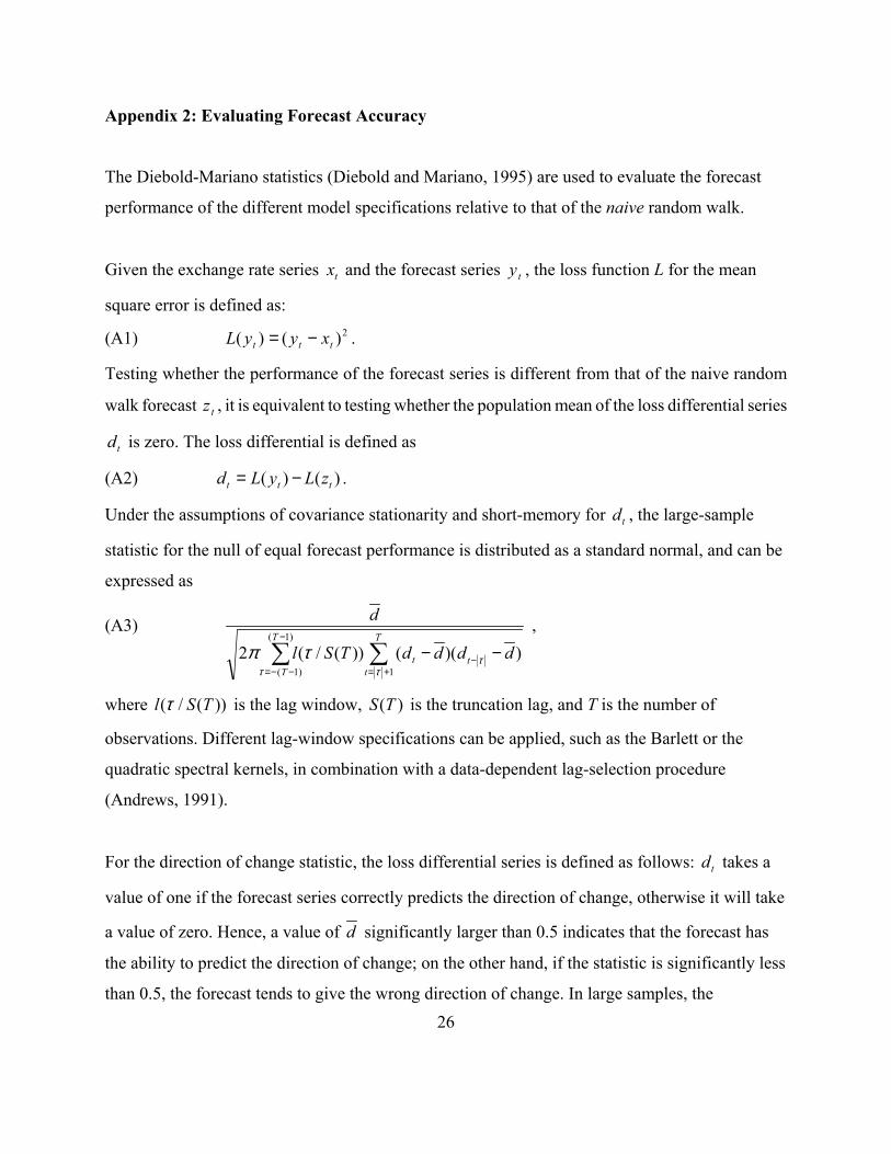
The Diebold-Mariano statistics (Diebold and Mariano, 1995) are used to evaluate the forecast
performance of the different model specifications relative to that of the naive random walk.
Given the exchange rate series tx and the forecast series ty , the loss function L for the mean
square error is defined as:
(A1) 2)()( ttt x y yL −= .
Testing whether the performance of the forecast series is different from that of the naive random
walk forecast tz , it is equivalent to testing whether the population mean of the loss differential series
td is zero. The loss differential is defined as
(A2) )()( ttt zLyLd −= .
Under the assumptions of covariance stationarity and short-memory for td , the large-sample
statistic for the null of equal forecast performance is distributed as a standard normal, and can be
expressed as
(A3) ddddTSl
d T
ttt
T
T∑∑
+=−
−
−−=
−−1
)1(
)1(
))(())(/(2τ
ττ
τπ,
where ))(/( TSl τ is the lag window, )(TS is the truncation lag, and T is the number of
observations. Different lag-window specifications can be applied, such as the Barlett or the
quadratic spectral kernels, in combination with a data-dependent lag-selection procedure
(Andrews, 1991).
For the direction of change statistic, the loss differential series is defined as follows: td takes a
value of one if the forecast series correctly predicts the direction of change, otherwise it will take
a value of zero. Hence, a value of d significantly larger than 0.5 indicates that the forecast has
the ability to predict the direction of change; on the other hand, if the statistic is significantly less
than 0.5, the forecast tends to give the wrong direction of change. In large samples, the

27
studentized version of the test statistic,
(A4) T
d /25.05.0− ,
is distributed as a standard Normal.
1
Table 1: The MSE Ratios from the Dollar-Based Exchange Rates Sample 1: 1987 Q2 - 2000 Q4 Sample 2: 1983 Q1-2000 Q4 Specification Horizon S-P IRP PROD BEER S-P IRP PROD BEER Panel A: BP/$ ECM 1 1.0465 1.0081 0.9954 1.0853 1.0499 1.0455 1.0418 1.0487 0.4089 0.8832 0.8968 0.2083 0.3098 0.3183 0.3030 0.4484 4 1.1273 1.0918 1.0169 1.0993 1.1416 1.1228 1.0850 1.1272 0.5031 0.6204 0.8022 0.2532 0.1714 0.3095 0.2369 0.2245 20 1.8089 1.3421 1.0953 1.3395 1.4568 0.8406 1.5450 2.1793 0.0143 0.2402 0.4109 0.1684 0.0707 0.5178 0.0918 0.0570 FD 1 1.0411 1.0055 1.1914 1.0858 1.0792 1.0230 0.4337 0.9399 0.2167 0.1345 0.3367 0.9010 4 1.1195 1.1235 1.8806 1.2498 1.4551 1.4476 0.3147 0.5237 0.0008 0.1487 0.1755 0.3510 20 1.8908 2.5310 6.9525 3.2231 5.5574 6.0151 0.1769 0.0205 0.0000 0.1953 0.0189 0.0013 Panel B: CAN$/$ ECM 1 1.0540 1.0903 1.1480 1.2783 1.0560 1.0920 1.0409 1.3371 0.1265 0.0477 0.0622 0.0157 0.2789 0.0216 0.5523 0.0037 4 1.1018 1.1722 1.1815 1.6025 1.1161 1.1696 1.0165 1.7540 0.1808 0.4516 0.1571 0.1183 0.3342 0.3589 0.9290 0.0175 20 0.9394 0.8649 1.0903 1.7595 1.0615 0.8128 1.0970 1.6233 0.5741 0.7602 0.3084 0.0018 0.7268 0.6072 0.3184 0.0001 FD 1 1.0998 1.1145 0.6144 1.1009 1.1708 0.6662 0.1789 0.1381 0.1094 0.2573 0.0469 0.1513 4 1.1367 1.1604 0.8993 1.1957 1.2688 1.1431 0.4605 0.3413 0.7980 0.3470 0.1923 0.7041 20 0.5152 0.5041 1.9236 1.8924 2.0043 2.2886 0.1931 0.1816 0.0058 0.1824 0.1427 0.2043 Panel C: DM/$ ECM 1 1.0589 1.0302 1.0413 0.9951 1.1047 1.0285 0.9965 0.9109 0.4642 0.2949 0.5737 0.9554 0.4157 0.3636 0.9614 0.2059 4 1.0804 1.1363 1.0799 1.1156 1.1040 1.0627 0.9487 0.8976 0.4444 0.0690 0.2820 0.6423 0.5986 0.4853 0.6255 0.5576 20 1.0467 0.5960 1.1311 2.1370 1.7712 0.8953 1.2596 0.6330 0.6367 0.1672 0.1411 0.2159 0.2121 0.6561 0.0393 0.2018 FD 1 1.2675 1.3235 0.5553 1.1225 1.1963 0.6941 0.0516 0.1059 0.0013 0.0169 0.0844 0.0203 4 1.4024 1.6067 0.8438 1.0765 1.2808 1.1513 0.0243 0.0300 0.5710 0.4524 0.0093 0.6117 20 1.8136 1.9266 2.5215 1.7226 1.9640 3.9752 0.1750 0.1139 0.1396 0.2459 0.1212 0.0025

2
Table 1 (Continued) Sample 1: 1987 Q2 - 2000 Q4 Sample 2: 1983 Q1-2000 Q4 Specification Horizon S-P IRP PROD BEER S-P IRP PROD BEER Panel D: SF/$ ECM 1 1.0741 1.0511 1.0238 . 0.9945 1.0497 1.0516 . 0.1868 0.1384 0.5152 . 0.9062 0.1408 0.5811 . 4 1.2689 1.1832 1.1844 . 1.0019 1.1220 1.1362 . 0.0148 0.0589 0.3666 . 0.9816 0.2477 0.1486 . 20 1.6208 1.4894 0.9694 . 1.3665 1.4894 1.3774 . 0.0685 0.0000 0.9335 . 0.0456 0.0000 0.0107 . FD 1 1.1057 1.0904 . 1.0886 1.0672 . 0.1889 0.3506 . 0.2373 0.5446 . 4 1.3615 1.4677 . 1.2321 1.3318 . 0.0037 0.0005 . 0.1532 0.0501 . 20 2.4774 2.6569 . 1.5404 1.8696 . 0.0394 0.0491 . 0.5211 0.3938 . Panel E: Yen/$ ECM 1 1.0672 1.0494 1.0726 . 1.0079 1.0321 1.0637 . 0.3115 0.2508 0.1249 . 0.9199 0.3607 0.2814 . 4 1.1894 1.1742 1.2391 . 1.0152 1.0482 1.2340 . 0.2791 0.2474 0.1507 . 0.8744 0.6580 0.0035 . 20 0.9508 0.6030 1.0110 . 1.1752 0.5661 1.2349 . 0.6470 0.2268 0.8510 . 0.0489 0.1737 0.0759 . FD 1 1.0852 1.0481 . 1.1647 1.1412 . 0.3211 0.4804 . 0.1790 0.2196 . 4 1.0039 1.0233 . 0.9937 1.0116 . 0.9776 0.8814 . 0.9686 0.9286 . 20 1.0808 0.9725 . 0.9236 1.0230 . 0.9122 0.9627 . 0.8439 0.9566 .
Note: The results are based on dollar-based exchange rates and their forecasts. Each cell in the Table has two entries. The first one is the MSE ratio (the MSEs of a structural model to the random walk specification). The entry underneath the MSE ratio is the p-value of the hypothesis that the MSEs of the structural and random walk models are the same (Diebold and Mariano, 1995). The notation used in the table is ECM: error correction specification; FD: first-difference specification; S-P: sticky-price model; IRP: interest rate parity model; PROD: productivity differential model; and BEER: behavioral equilibrium exchange rate model. The forecasting horizons (in quarters) are listed under the heading “Horizon.” The results for the post-Louvre Accord forecasting period are given under the label “Sample 1” and those for the post-1983 forecasting period are given under the label “Sample 2.” A "." indicates the statistics are not generated due to unavailability of data.
3
Table 2: The MSE Ratios from the Yen-Based Exchange Rates Sample 1: 1987 Q2 - 2000 Q4 Sample 2: 1983 Q1-2000 Q4 Specification Horizon S-P IRP PROD S-P IRP PROD Panel A: BP/Yen ECM 1 0.9937 1.0363 1.0873 1.0438 0.9955 1.0471 0.8585 0.6407 0.3347 0.1254 0.9456 0.5705 4 1.0311 1.0643 1.1094 1.0990 0.9337 1.0068 0.7357 0.7596 0.5603 0.1771 0.6834 0.9529 20 1.2997 0.6422 1.2172 0.7305 0.5262 0.8828 0.0147 0.2453 0.1281 0.0898 0.1260 0.4380 FD 1 1.0272 1.0412 0.9608 0.9515 0.7921 0.6781 0.6825 0.6254 4 1.1758 1.2496 0.8327 0.8315 0.4654 0.3569 0.4272 0.4115 20 1.8800 2.1663 1.4420 1.5873 0.3738 0.3302 0.5831 0.4870 Panel B: CAN$/Yen ECM 1 1.1569 1.0225 1.0830 1.0244 0.9964 0.9827 0.1101 0.6270 0.0505 0.8506 0.9252 0.8502 4 1.3197 1.0679 1.0916 1.0386 0.9561 1.1492 0.1194 0.7063 0.2399 0.8085 0.7305 0.1427 20 1.2658 0.5416 1.0806 1.2267 0.4774 1.3773 0.0873 0.0562 0.4042 0.1715 0.0353 0.2400 FD 1 1.0497 1.0193 1.0092 0.9950 0.5369 0.8017 0.9199 0.9510 4 1.0918 1.0984 0.7931 0.8635 0.6933 0.7169 0.3591 0.5372 20 0.8840 0.8338 1.0639 1.3366 0.8657 0.8156 0.9239 0.6536
Panel C: US$/Yen ECM 1 1.0672 1.0494 1.0726 1.0079 1.0321 1.0637 0.3115 0.2508 0.1249 0.9199 0.3607 0.2814 4 1.1894 1.1742 1.2391 1.0152 1.0482 1.2340 0.2791 0.2474 0.1507 0.8744 0.6580 0.0035 20 0.9508 0.6030 1.0110 1.1752 0.5661 1.2349 0.6470 0.2268 0.8510 0.0489 0.1737 0.0759 FD 1 1.0852 1.0481 1.1647 1.1412 0.3211 0.4804 0.1790 0.2196 4 1.0039 1.0233 0.9937 1.0116 0.9776 0.8814 0.9686 0.9286 20 1.0808 0.9725 0.9236 1.0230 0.9122 0.9627 0.8439 0.9566
4
Table 2: (Continued) Sample 1: 1987 Q2 - 2000 Q4 Sample 2: 1983 Q1-2000 Q4 Specification Horizon S-P IRP PROD S-P IRP PROD Panel D: DM/Yen ECM 1 0.9882 0.9858 1.0186 1.0335 0.9937 0.9836 0.6016 0.7052 0.4558 0.4178 0.8554 0.6381 4 0.9604 0.9323 1.0319 0.9904 0.9438 0.9871 0.1189 0.5087 0.6289 0.8168 0.5297 0.8153 20 1.0053 0.6494 1.0086 1.1873 0.6701 1.0031 0.7024 0.0356 0.8930 0.3738 0.0179 0.9614 FD 1 1.1431 1.0877 1.1767 1.0955 0.0966 0.3007 0.0161 0.0806 4 1.1719 1.0955 1.1975 1.1395 0.0656 0.2848 0.0826 0.0991 20 1.0127 1.1023 1.4901 1.5938 0.9242 0.5934 0.3031 0.1752 Panel E: SF/Yen ECM 1 0.9573 1.0167 1.0940 1.0337 1.0311 1.1280 0.4350 0.4571 0.1051 0.5142 0.1588 0.0392 4 0.9658 0.9856 1.2521 1.0675 1.0288 1.1710 0.5579 0.8259 0.0011 0.2250 0.6722 0.1262 20 0.9443 0.9031 1.1902 1.1598 0.9031 1.2034 0.2164 0.4856 0.2661 0.1405 0.4856 0.0194 FD 1 1.0696 1.0168 1.2217 1.1857 0.3140 0.8153 0.0490 0.1221 4 1.1656 1.1169 1.2514 1.1894 0.0629 0.1195 0.0791 0.0572 20 1.7151 1.6450 1.5828 1.6124 0.2592 0.2264 0.1737 0.1271
Note: The results are based on yen-based exchange rates and their forecasts. Each cell in the Table has two entries. The first one is the MSE ratio (the MSEs of a structural model to the random walk specification). The entry underneath the MSE ratio is the p-value of the hypothesis that the MSEs of the structural and random walk models are the same (Diebold and Mariano, 1995). The notation used in the table is ECM: error correction specification; FD: first-difference specification; S-P: sticky-price model; IRP: interest rate parity model; PROD: productivity differential model; and BEER: behavioral equilibrium exchange rate model. The forecasting horizons (in quarters) are listed under the heading “Horizon.” The results for the post-Louvre Accord forecasting period are given under the label “Sample 1” and those for the post-1983 forecasting period are given under the label “Sample 2.”

5
Table 3: Direction of Change Statistics from the Dollar-Based Exchange Rates Sample 1: 1987 Q2 - 2000 Q4 Sample 2: 1983 Q1-2000 Q4 Specification Horizon S-P IRP PROD BEER S-P IRP PROD BEER Panel A: BP/$ ECM 1 0.5455 0.4643 0.5636 0.5273 0.5694 0.4110 0.5278 0.5278 0.5002 0.5930 0.3452 0.6858 0.2386 0.1281 0.6374 0.6374 4 0.5769 0.5000 0.5192 0.4808 0.5217 0.4247 0.4638 0.5073 0.2673 1.0000 0.7815 0.7815 0.7180 0.1979 0.5472 0.9042 20 0.3889 0.5357 0.4722 0.3611 0.5094 0.5890 0.4906 0.3585 0.1824 0.5930 0.7389 0.0956 0.8908 0.1281 0.8908 0.0394 FD 1 0.4546 0.4727 0.4182 0.4722 0.5000 0.5556 0.5002 0.6858 0.2249 0.6374 1.0000 0.3458 4 0.4808 0.5769 0.3654 0.5073 0.6667 0.5362 0.7815 0.2673 0.0522 0.9042 0.0056 0.5472 20 0.6389 0.5556 0.5000 0.4151 0.4528 0.4906 0.0956 0.5050 1.0000 0.2164 0.4922 0.8908 Panel B: CAN$/$ ECM 1 0.4727 0.4286 0.4000 0.3818 0.5139 0.4247 0.5000 0.4583 0.6858 0.2851 0.1380 0.0796 0.8137 0.1979 1.0000 0.4795 4 0.4423 0.3393 0.4231 0.3462 0.5362 0.3699 0.5942 0.3188 0.4054 0.0162 0.2673 0.0265 0.5472 0.0262 0.1176 0.0026 20 0.5000 0.7321 0.4722 0.0833 0.4717 0.7671 0.5094 0.1509 1.0000 0.0005 0.7389 0.0000 0.6803 0.0000 0.8908 0.0000 FD 1 0.5091 0.4727 0.6182 0.5417 0.4444 0.6111 0.8927 0.6858 0.0796 0.4795 0.3458 0.0593 4 0.5385 0.5192 0.6731 0.4783 0.4928 0.6232 0.5791 0.7815 0.0126 0.7180 0.9042 0.0407 20 0.8889 0.8889 0.5833 0.5849 0.6038 0.5094 0.0000 0.0000 0.3173 0.2164 0.1308 0.8908 Panel C: DM/$ ECM 1 0.6364 0.3571 0.4546 0.4909 0.4861 0.4110 0.5000 0.4861 0.0431 0.0325 0.5002 0.8927 0.8137 0.1281 1.0000 0.8137 4 0.6346 0.4286 0.4615 0.4615 0.4493 0.4247 0.4493 0.5073 0.0522 0.2851 0.5791 0.5791 0.3994 0.1979 0.3994 0.9042 20 0.5833 0.6964 0.3333 0.3333 0.2830 0.5890 0.4340 0.5094 0.3173 0.0033 0.0455 0.0455 0.0016 0.1281 0.3363 0.8908 FD 1 0.4546 0.4727 0.8000 0.4444 0.4444 0.7500 0.5002 0.6858 0.0000 0.3458 0.3458 0.0000 4 0.3654 0.4615 0.6731 0.4928 0.4493 0.6087 0.0522 0.5791 0.0126 0.9042 0.3994 0.0710 20 0.6111 0.6389 0.6667 0.5094 0.4151 0.4717 0.1824 0.0956 0.0455 0.8908 0.2164 0.6803

6
Table 3: (Continued) Sample 1: 1987 Q2 - 2000 Q4 Sample 2: 1983 Q1-2000 Q4 Specification Horizon S-P IRP PROD BEER S-P IRP PROD BEER Panel D: SF/$ ECM 1 0.4000 0.3393 0.6182 . 0.5417 0.3836 0.6250 . 0.1380 0.0162 0.0796 . 0.4795 0.0466 0.0339 . 4 0.4039 0.4107 0.5385 . 0.5797 0.4247 0.5797 . 0.1655 0.1815 0.5791 . 0.1854 0.1979 0.1854 . 20 0.4444 0.4546 0.5833 . 0.5283 0.4546 0.4340 . 0.5050 0.6698 0.3173 . 0.6803 0.6698 0.3363 . FD 1 0.4364 0.4000 . 0.4444 . 0.4583 . 0.3452 0.1380 . 0.3458 . 0.4795 . 4 0.3462 0.3077 . 0.4348 . 0.3623 . 0.0265 0.0055 . 0.2786 . 0.0222 . 20 0.6111 0.6111 . 0.7170 . 0.6981 . 0.1824 0.1824 . 0.0016 . 0.0039 . Panel E: Yen/$ ECM 1 0.5273 0.3750 0.5455 . 0.5972 0.4247 0.5139 . 0.6858 0.0614 0.5002 . 0.0990 0.1979 0.8137 . 4 0.5769 0.4821 0.5192 . 0.6232 0.5480 0.4058 . 0.2673 0.7893 0.7815 . 0.0407 0.4126 0.1176 . 20 0.5556 0.6964 0.5556 . 0.4151 0.7031 0.3396 . 0.5050 0.0033 0.5050 . 0.2164 0.0012 0.0195 . FD 1 0.5818 0.5636 . 0.5833 0.5417 . 0.2249 0.3452 . 0.1573 0.4795 . 4 0.6539 0.5962 . 0.6522 0.6522 . 0.0265 0.1655 . 0.0115 0.0115 . 20 0.6111 0.5833 . 0.7547 0.7359 . 0.1824 0.3173 . 0.0002 0.0006 .
Note: Table 3 reports the proportion of forecasts that correctly predict the direction of the dollar exchange rate movement. Underneath each direction of change statistic, the p-values for the hypothesis that the reported proportion is significantly different from ½ is listed. When the statistic is significantly larger than ½, the forecast is said to have the ability to predict the direct of change. If the statistic is significantly less than ½, the forecast tends to give the wrong direction of change. The notation used in the table is ECM: error correction specification; FD: first-difference specification; S-P: sticky-price model; IRP: interest rate parity model; PROD: productivity differential model; and BEER: behavioral equilibrium exchange rate model. The forecasting horizons (in quarters) are listed under the heading “Horizon.” The results for the post-Louvre Accord forecasting period are given under the label “Sample 1” and those for the post-1983 forecasting period are given under the label “Sample 2.” A "." indicates the statistics are not generated due to unavailability of data.

7
Table 4: Direction of Change Statistics from the Yen-Based Exchange Rates Sample 1: 1987 Q2 - 2000 Q4 Sample 2: 1983 Q1-2000 Q4 Specification Horizon S-P IRP PROD S-P IRP PROD Panel A: BP/Yen ECM 1 0.4546 0.4286 0.5091 0.3889 0.5069 0.4861 0.5002 0.2851 0.8927 0.0593 0.9068 0.8137 4 0.5000 0.6429 0.5192 0.4058 0.7123 0.5073 1.0000 0.0325 0.7815 0.1176 0.0003 0.9042 20 0.3611 0.7143 0.5278 0.6226 0.7500 0.5660 0.0956 0.0013 0.7389 0.0742 0.0001 0.3363 FD 1 0.5455 0.5091 0.5278 0.5417 0.5002 0.8927 0.6374 0.4795 4 0.6346 0.6346 0.6957 0.7391 0.0522 0.0522 0.0012 0.0001 20 0.6111 0.6111 0.7170 0.7170 0.1824 0.1824 0.0016 0.0016 Panel B: CAN$/Yen ECM 1 0.5455 0.5000 0.4364 0.5833 0.5343 0.5278 0.5002 1.0000 0.3452 0.1573 0.5584 0.6374 4 0.4808 0.5893 0.4615 0.5797 0.6438 0.5362 0.7815 0.1815 0.5791 0.1854 0.0140 0.5472 20 0.4167 0.7679 0.4444 0.4528 0.7969 0.5283 0.3173 0.0001 0.5050 0.4922 0.0000 0.6803 FD 1 0.5091 0.5091 0.4722 0.5000 0.8927 0.8927 0.6374 1.0000 4 0.5385 0.5769 0.6377 0.6232 0.5791 0.2673 0.0222 0.0407 20 0.6944 0.6944 0.7359 0.7170 0.0196 0.0196 0.0006 0.0016 Panel C: US$/Yen ECM 1 0.5273 0.3750 0.5455 0.5972 0.4247 0.5139 0.6858 0.0614 0.5002 0.0990 0.1979 0.8137 4 0.5769 0.4821 0.5192 0.6232 0.5480 0.4058 0.2673 0.7893 0.7815 0.0407 0.4126 0.1176 20 0.5556 0.6964 0.5556 0.4151 0.7031 0.3396 0.5050 0.0033 0.5050 0.2164 0.0012 0.0195 FD 1 0.5818 0.5636 0.5833 0.5417 0.2249 0.3452 0.1573 0.4795 4 0.6539 0.5962 0.6522 0.6522 0.0265 0.1655 0.0115 0.0115 20 0.6111 0.5833 0.7547 0.7359 0.1824 0.3173 0.0002 0.0006
8
Table 4: (Continued)
Sample 1: 1987 Q2 - 2000 Q4 Sample 2: 1983 Q1-2000 Q4
Specification Horizon S-P IRP PROD S-P IRP PROD Panel D: DM/Yen ECM 1 0.6000 0.4464 0.6546 0.4306 0.4247 0.6111 0.1380 0.4227 0.0219 0.2386 0.1979 0.0593 4 0.4615 0.5357 0.4808 0.5073 0.5206 0.5217 0.5791 0.5930 0.7815 0.9042 0.7255 0.7180 20 0.4444 0.7143 0.5556 0.5283 0.7188 0.6226 0.5050 0.0013 0.5050 0.6803 0.0005 0.0742 FD 1 0.4546 0.5091 0.4861 0.5139 0.5002 0.8927 0.8137 0.8137 4 0.4039 0.4808 0.4928 0.5362 0.1655 0.7815 0.9042 0.5472 20 0.6111 0.6111 0.5660 0.4528 0.1824 0.1824 0.3363 0.4922 Panel E: SF/Yen ECM 1 0.6182 0.5179 0.4182 0.5972 0.4384 0.5139 0.0796 0.7893 0.2249 0.0990 0.2922 0.8137 4 0.5192 0.4643 0.3077 0.4783 0.3973 0.4493 0.7815 0.5930 0.0055 0.7180 0.0792 0.3994 20 0.5278 0.5000 0.5000 0.3962 0.5000 0.3396 0.7389 1.0000 1.0000 0.1308 1.0000 0.0195 FD 1 0.4727 0.4909 0.4722 0.5000 0.6858 0.8927 0.6374 1.0000 4 0.4615 0.5192 0.5217 0.4493 0.5791 0.7815 0.7180 0.3994 20 0.6944 0.6944 0.6038 0.4906 0.0196 0.0196 0.1308 0.8908
Note: Table 4 reports the proportion of forecasts that correctly predict the direction of the yen-based exchange rate movement. Underneath each direction of change statistic, the p-values for the hypothesis that the reported proportion is significantly different from ½ is listed. When the statistic is significantly larger than ½, the forecast is said to have the ability to predict the direct of change. If the statistic is significantly less than ½, the forecast tends to give the wrong direction of change. The notation used in the table is ECM: error correction specification; FD: first-difference specification; S-P: sticky-price model; IRP: interest rate parity model; PROD: productivity differential model; and BEER: behavioral equilibrium exchange rate model. The forecasting horizons (in quarters) are listed under the heading “Horizon.” The results for the post-Louvre Accord forecasting period are given under the label “Sample 1” and those for the post-1983 forecasting period are given under the label “Sample 2.”
9
Table 5: Cointegration between Dollar-Based Exchange Rates and their Forecasts Sample 1: 1987 Q2 - 2000 Q4 Sample 2: 1983 Q1-2000 Q4 Specification Horizon S-P IRP PROD BEER S-P IRP PROD BEER Panel A: BP/$ ECM 1 7.26 0.77 6.95 12.64* 17.09* 4.60 10.40* 32.83* 4 8.56 1.47 9.66* 84.86* 12.98* 3.77 7.88 18.94* 20 15.84* 5.30 18.82* 6.95 3.16 5.03 4.25 4.72 FD 1 25.63* 20.85* 13.03* 34.00* 8.60 16.91* 4 7.30 6.71 2.21 6.98 3.02 3.45 20 8.45 13.00* 3.44 3.57 2.79 2.24 Panel B: CAN$/US$ ECM 1 11.64* 1.29 4.37 10.35* 14.31* 1.90 13.96* 19.66* 4 10.27* 2.53 4.55 5.39 6.37 1.53 9.58* 13.52* 20 15.02* 3.98 19.82* 9.67* 2.61 4.18 1.60 2.19 FD 1 26.34* 31.53* 9.19 25.72* 9.89* 8.12 4 3.19 3.87 3.88 6.99 8.63 3.89 20 10.03* 9.59* 6.72 1.45 2.21 3.52 Panel C: DM/$ ECM 1 3.67 5.19 3.86 5.23 12.68* 2.84 27.29* 21.03* 4 5.24 2.74 5.37 18.33* 24.06* 1.81 6.67 8.49 20 6.09 1.63 7.55 9.20 3.56 2.37 2.94 16.60* FD 1 20.82* 4.02 8.29 36.32* 35.91* 2.18 4 4.27 3.16 15.29* 7.56 10.82* 2.80 20 5.42 8.62 3.74 3.69 4.16 4.26 Panel D: SF/$ ECM 1 6.75 3.45 3.80 . 22.10* 3.23 6.33 . 4 8.55 2.07 9.10 . 10.71* 2.27 9.68* . 20 1.16 6.93 1.81 . 2.93 6.93 2.96 . FD 1 33.01* 20.30* . 23.55* 10.38* . 4 10.96* 6.71 . 14.33* 13.74* . 20 9.43 7.51 . 2.27 2.59 . Panel E: Yen/$ ECM 1 2.19 6.94 1.84 . 19.44* 6.45 12.73* . 4 3.43 4.13 3.22 . 10.71* 3.27 14.79* . 20 4.67 2.93 2.19 . 2.90 3.48 5.63 . FD 1 13.35* 9.79* . 15.47* 15.47* . 4 5.53 3.77 . 6.02 5.74 . 20 1.76 2.15 . 4.94 3.96 .

10
Note: The Johansen maximum eigenvalue statistic for the null hypothesis that a dollar-based exchange rate and its forecast are no cointegrated. "*" indicates 10% level significance. Tests for the null of one cointegrating vector were also conducted but in all cases the null was not rejected. The notation used in the table is ECM: error correction specification; FD: first-difference specification; S-P: sticky-price model; IRP: interest rate parity model; PROD: productivity differential model; and BEER: behavioral equilibrium exchange rate model. The forecasting horizons (in quarters) are listed under the heading “Horizon.” The results for the post-Louvre Accord forecasting period are given under the label “Sample 1” and those for the post-1983 forecasting period are given under the label “Sample 2.” A "." indicates the statistics are not generated due to unavailability of data.

11
Table 6: Cointegration between Yen-Based Exchange Rates and their Forecasts Sample 1: 1987 Q2 - 2000 Q4 Sample 2: 1983 Q1-2000 Q4 Specification Horizon S-P IRP PROD S-P IRP PROD Panel A: BP/Yen ECM 1 2.60 9.79* 3.53 8.63 11.05* 4.06 4 2.68 7.66 1.92 8.72 9.79* 6.30 20 3.88 5.71 4.29 8.33 3.32 9.55* FD 1 38.24* 46.93* 43.12* 43.65* 4 13.81* 13.23* 13.50* 17.52* 20 2.32 2.25 3.47 3.83 Panel B: CAN$/Yen ECM 1 7.66 10.07* 12.62* 16.52* 15.42* 15.32* 4 7.55 10.29* 9.31 11.40* 11.11* 40.72* 20 2.81 11.04* 4.50 5.36 11.97* 4.61 FD 1 31.03* . 32.75* 21.00* . 38.87* 4 5.14 . 5.05 6.86 . 5.38 20 6.20 . 2.72 3.60 . 5.29 Panel C: US$/Yen ECM 1 2.19 6.94 1.84 19.44* 6.45 12.73* 4 3.43 4.13 3.22 10.71* 3.27 14.79* 20 4.67 2.93 2.19 2.90 3.48 5.63 FD 1 13.35* 9.79* 15.47* 15.47* 4 5.53 3.77 6.02 5.74 20 1.76 2.15 4.94 3.96 Panel D: DM/Yen ECM 1 25.38* 6.64 27.61* 32.48* 2.62 31.34* 4 14.29* 5.43 11.08* 14.18* 2.24 13.96* 20 13.99 7.60 5.39 16.07* 8.82 16.79* FD 1 23.07* 28.73* 37.69* 17.57* 4 15.19* 11.27* 5.91 4.63 20 19.61* 19.21* 4.82 4.75 Panel E: SF/Yen ECM 1 7.50* 20.19* 13.16* 26.65* 5.46 22.58* 4 4.36 4.39 7.72 115.2* 2.81 9.02 20 5.02 4.72 5.87 6.58 4.72 6.16 FD 1 45.52* 48.77* 50.81* 55.40* 4 9.69* 10.98* 10.99 11.72* 20 4.55 4.80 6.21 5.60

12
Note: The Johansen maximum eigenvalue statistic for the null hypothesis that a yen-based exchange rate and its forecast are no cointegrated. "*" indicates 10% level significance. Tests for the null of one cointegrating vector were also conducted but in all cases the null was not rejected. The notation used in the table is ECM: error correction specification; FD: first-difference specification; S-P: sticky-price model; IRP: interest rate parity model; PROD: productivity differential model; and BEER: behavioral equilibrium exchange rate model. The forecasting horizons (in quarters) are listed under the heading “Horizon.” The results for the post-Louvre Accord forecasting period are given under the label “Sample 1” and those for the post-1983 forecasting period are given under the label “Sample 2.”

13
Table 7: Results of the (1, -1) Restriction Test: Dollar-Based Exchange Rates Sample 1: 1987 Q2 - 2000 Q4 Sample 2: 1983 Q1-2000 Q4 Specification Horizon S-P IRP PROD BEER S-P IRP PROD BEER Panel A: BP/$ ECM 1 0.55 3.38 0.00 0.35 0.46 0.07 1.00 0.56 4 0.98 1.02 2.59 0.09 0.32 0.31 0.11 0.76 20 0.40 0.36 0.53 0.55 FD 1 5.38 0.12 0.04 0.79 0.36 0.02 0.73 0.83 0.38 0.55 4 20 23.20 0.00 Panel B: CAN$/$ ECM 1 11.20 4.46 7.75 2.87 6.48 0.00 0.03 0.01 0.09 0.01 4 24.05 5.36 4.52 0.00 0.02 0.03 20 76.59 82.26 201.37 0.00 0.00 0.00 FD 1 7.81 6.09 13.90 5.47 0.01 0.01 0.00 0.02 4 20 4.39 3.50 0.04 0.06 Panel C: DM/$ ECM 1 8.82 8.35 6.61 0.00 0.00 0.01 4 3.20 6.31 0.07 0.01 20 27.81 0.00 FD 1 10.17 3.03 0.47 0.00 0.08 0.49 4 25.21 7.39 0.00 0.01 20

14
Table 7: (Continued) Sample 1: 1987 Q2 - 2000 Q4 Sample 2: 1983 Q1-2000 Q4 Specification Horizon S-P IRP PROD BEER S-P IRP PROD BEER Panel D: SF/$ . . ECM 1 . 10.07 . . 0.00 . 4 . 2.40 10.96 . . 0.12 0.00 . 20 . . . . FD 1 20.17 20.82 . 4.57 4.79 . 0.00 0.00 . 0.03 0.03 . 4 20.87 . 8.84 8.40 . 0.00 . 0.00 0.00 . 20 . . . . Panel E: Yen/$ ECM 1 . 3.22 2.47 . . 0.07 0.12 . 4 . 0.55 5.71 . . 0.46 0.02 . 20 . . . . FD 1 6.76 5.40 . 0.45 0.71 . 0.01 0.02 . 0.50 0.40 . 4 . . . . 20 . . . .
Note: The likelihood ratio test statistic for the restriction of (1, -1) on the cointegrating vector and its p-value are reported. The test is only applied to the cointegration cases present in Table 5. The notation used in the table is ECM: error correction specification; FD: first-difference specification; S-P: sticky-price model; IRP: interest rate parity model; PROD: productivity differential model; and BEER: behavioral equilibrium exchange rate model. The forecasting horizons (in quarters) are listed under the heading “Horizon.” The results for the post-Louvre Accord forecasting period are given under the label “Sample 1” and those for the post -1983 forecasting period are given under the label “Sample 2.” A "." indicates the statistics are not generated due to unavailability of data.
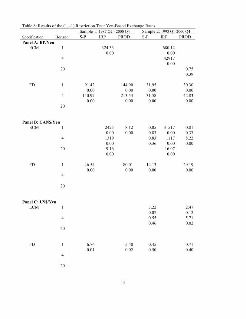
15
Table 8: Results of the (1, -1) Restriction Test: Yen-Based Exchange Rates Sample 1: 1987 Q2 - 2000 Q4 Sample 2: 1993 Q1-2000 Q4 Specification Horizon S-P IRP PROD S-P IRP PROD Panel A: BP/Yen ECM 1 324.33 680.12 0.00 0.00 4 42917 0.00 20 0.75 0.39 FD 1 91.42 144.90 31.95 30.30 0.00 0.00 0.00 0.00 4 140.97 213.53 31.58 42.83 0.00 0.00 0.00 0.00 20 Panel B: CAN$/Yen ECM 1 2425 8.12 0.05 31517 0.81 0.00 0.00 0.83 0.00 0.37 4 1319 0.83 1117 8.22 0.00 0.36 0.00 0.00 20 9.16 16.07 0.00 0.00 FD 1 46.54 80.01 14.13 29.19 0.00 0.00 0.00 0.00 4 20 Panel C: US$/Yen ECM 1 3.22 2.47 0.07 0.12 4 0.55 5.71 0.46 0.02 20 FD 1 6.76 5.40 0.45 0.71 0.01 0.02 0.50 0.40 4 20

16
Table 8: (Continued) Sample 1: 1987 Q2 - 2000 Q4 Sample 2: 1983 Q1-2000 Q4 Specification Horizon S-P IRP PROD S-P IRP PROD Panel D: DM/Yen ECM 1 0.01 0.06 0.51 0.36 0.93 0.80 0.47 0.54 4 1.12 0.97 0.51 0.55 0.29 0.32 0.47 0.45 20 0.01 0.81 0.91 0.36 FD 1 2.67 4.90 13.80 7.02 0.10 0.03 0.00 0.00 4 4.84 6.87 0.03 0.00 20 24.04 19.86 0.00 0.00 Panel E: SF/Yen ECM 1 22.56 94.44 0.50 11.59 4.53 0.00 0.00 0.48 0.00 0.03 4 85.62 0.00 20 FD 1 6.85 5.82 4.16 3.82 0.01 0.02 0.04 0.05 4 14.41 11.31 2.29 0.00 0.00 0.13 20
Note: Note: The likelihood ratio test statistic for the restriction of (1, -1) on the cointegrating vector and its p-value are reported. The test is only applied to the cointegration cases present in Table 6. The notation used in the table is ECM: error correction specification; FD: first-difference specification; S-P: sticky-price model; IRP: interest rate parity model; PROD: productivity differential model; and BEER: behavioral equilibrium exchange rate model. The forecasting horizons (in quarters) are listed under the heading “Horizon.” The results for the post-Louvre Accord forecasting period are given under the label “Sample 1” and those for the post-1983 forecasting period are given under the label “Sample 2.”
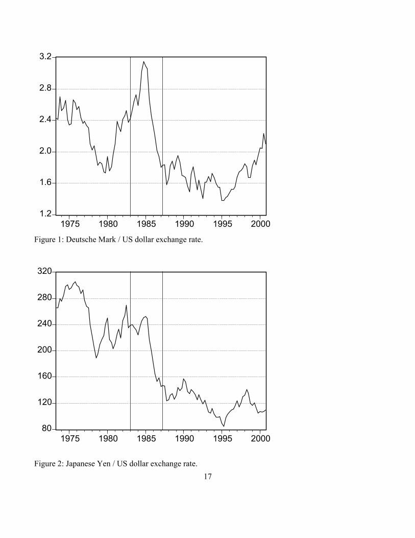
17
1.2
1.6
2.0
2.4
2.8
3.2
1975 1980 1985 1990 1995 2000
Figure 1: Deutsche Mark / US dollar exchange rate.
80
120
160
200
240
280
320
1975 1980 1985 1990 1995 2000
Figure 2: Japanese Yen / US dollar exchange rate.

18
-6.0
-5.6
-5.2
-4.8
-4.4
-4.0
-3.6
1975 1980 1985 1990 1995 2000
Actuallog (C$/Yen)
IRP(20-quarter)
Random Walk(20-quarter)
Figure 3: Canadian dollar / Yen actual, 20-quarter ahead interest rate parity and random walk forecasts.
Recommended