NAVAL POSTGRADUATE SCHOOLMonterey, California
ID
__ LECTEDEC 2 8 1989
THESISDOA ESTIMAION BY IIGENDFCO\IPOSI LION
L'SING SI\(iI 1E VEC ORI ACZ0S Al.GORITII\I
by
Danicl L. Gear
June 1989
Thesis Ad isor Muzali unrnala
Approved for public release; distribution is unlimited.
89 12 27 070

DIC0ll MMTIC~rI
THIS DOCUMENT IS BEST
QUALITY AVAILABLE. THE COPY
FURNISHED TO DTIC CONTAINED
A SIGNIFICANT NUMBER OF
PAGES WHICH DO NOTREPRODUCE LEGIBLY

Unclassifiedsecur! c : a i ,-J RIIPORIl DOCl\IENTAI ION 1PA(,
C22>c~' \.'rt 3 Di~riib:;on u.;~b! f Rep 0r
2 b DCL~zSSI!fCatmorIlw S- . Approx ed for public rcloascv: distiribhution 1 uiimitcd(.
4 nI Name of Performing %~::zc O:2cS\o a ne o" I o~O::oNaval Postaraduate School a, iri 6f_2 Naval IPosturaduato Schoolvc A-ddress tci-. sraf-. wid ZIP -~b Address O.siauw audXI' uJ
Nlnntcrev. CA 93941-5000( Monterey. CA 93Q43.511(1(Sa Name of Fundin.g Sp oc Or.,aou&. 1:Oc Sh Piocujremeni orr:I&::cznNmc
"C Addrcss ... saJae ZIP S o Su r c %,o un,'-.no N:
pro 2ram Liemlen:N I \C )roec. N :i . ~UT: .~...,.DOAX LS iI'l\1I ION\ BY I lGlINDl1COMPlOSITION liSIN~ SI \(iL \L FI OR
LANCY(1 AIS \GORIl 1*11l
N Liirs I helli For 10 qu e
- Su- r -~'- N ea:::. icxepicsscd 'in thil thcsir, arc 010oc oi thle author anld do( not ruIlct the ofiL il p toi, po,-
A Sub-, paccmthd of >o n ir'' r inad d'1irection of arrivaLI D .OA) prohlemsl involve: finii er1 i
anld Cil'cT.-ctar>, Of eon eCIliwn titne .~ th c I OOC/OS ale-othin117 >,ome of theL extrecieoaue a i e tr can'4be 1:a-m II x mt-d thlou ej1! : ik u tiru in itrix dcoirpomitioni theoreticaLly11 ic hOclptU~i
I Jcievlp a mod ' r1 1d a orm of the I afllzo> al'ortitl u to~ Col C he I11 )(\prea i p Of 1henuirlb':r at 'o-cecor i-c to thc acur.Ic\ of lc hereli a loaw -iunal to nioise, ratioexni arc XI li
D I)ri 1 010) )4'I",( %14 0,1 A
(_)classified

Approved for public release: distribution is unliniftcd.
DOA ESTEIAVIION BY EIGL\1)LCOMPOSII IONUSING SINGLE VIXC] ORLANCZOS ALGORI IJIM P
by
Daniel E. GearLieutenant Commander, . nited States Navy
A.B.. Liiix crsity of North Carolina, 1977
Submitted in partial fullillticrit of therequirements for the degree of
MIASIfER OF SC11l:NCE IN ELLCJI RICAL ENGINTERINGi
firom the
NAVAL POS rGRAM.'AIlF SCHOO001
JUNE 1989)
A utoir:
Daniel I.". Gear
A'pprovedi by:FX. -~~~~ t
Nfural] Tunmmka i. TherPk AdiseIr
Char les NV. I hci cn, Second Readcr
John P. Powers, Chairman,Department of Elecctrical and Computer Engineeringe
(jordJon E.Schjjcr.D~ean of Science and Engineeing1

ABSTRACT
Subspace methods of solving spectral estimation and direction of arrival (I)O\)problems involve finding the eigenvalues and eigenvectors of correlation matrices. Using
the Lanczos algorithm some of the extreme eigenvalucs and eigenvectors can be ap-
proximated without requiring the entire matrix dccomposition theoretically saving many
computations.
This thesis develops a model and a form of the Lanczos algorithm to solve the DOAproblem. The relationship of the number of cicenvectors used to the accur;1Lv of theresults in a low siunal to noise ratio example are examined.
S'.c cz:-;,:, F~r
U ,', , <Lit C ..
J ,-, T A3
By
Di st < U,1,y ('c. '
Ditii ~ ~ d

TABLE OF CONTENTS
1. IN TRO D U CTIO N .............................................. I
I1. DIRECTION OF ARRIVAL ..................................... 3
A. SPEC'IRAL LSTIM A'ION .................................... 3
B. BEA M FO RM IN G ........................................... 8
C. 3luISPACE NIIETIIO D S ...................................... 13
1. In tro d uctio n ............................................13
2. M U S IC ...............................................15
3. L S P R IT .... ....................................... ... . 18
4. O ther Subspace M ethods .................................. 21
III. e LANCZOS Al (I ORITIIM ................................. 22
A. C:LASSI(.,\L IANCZOS AND ITS VARiANTS ................... 23
B. IM PL .ILNTA TIO N ....................................... 27
1. Single Vector Lanczos Algorithn. ............................ 28
2. O ther M ethods ....................... ................... 39
IV . R ESI TS . ..................................................4 2
A . A PP R O A C I I .............................................. 4 2
B. EXPLR I.M I-NT SET UP ...................................... 43
V. CONCLUSIONS AND RIECOMMIENDATIONS ..................... 67
I1ST O F R I I : R L-N ( E S ........................................... 68
INITIAL )ISTRI BUTION LIST .................................... 72
iv

LIST OF FIGURES
Figure 1. W avefront .............................................. 9
Figure 2. Simple de!av-and-sum bean-former ................. ......... 10
Figure 3. Spatial Frequency . ....................................... 12
Figure 4. Steering vector for 3 sensors and I signal ...................... 16
Figure 5. Signal Subspace for 2 signals ............................... 17
Figure 6. PSD offirst eigenvector . ................................... 32
FiLure 7. PSD of second eigenvector ................................. 33
Ficure 8. Overlaved PSDs of first 5 cicenvector ......................... 34
1t uu 9. Eigenvector averaging .......................................
lig ure 1 . Spectral avcraging .......................................... .:
I-i,,:UrC 11. Spectral product for 2 ejicnvectors ............ .............1:igLire 12. Spectral product for 5 ejeenvectors .............................Sb
Figure 13. Spectral product for 5 cicenvcctors, 0dB ...................... "-
Fire 1,4. Spectral product for 5 eLgencjctor. - ( d . 17
Iigu: 15. Spectral product for 5 ei envc Ctors, -5 dB ...................... -S
Fig i e 16. Spectral product f(or 10 eic cn c:torl. -5 dB ...................... IS
FigLre I1. Spectral product for 15 cigCnvcctors, -5 dB ..................... 3 k
I igure 1S. \ ph"s ical implemcntation. ................................... 4
Figure 1 9. Case 1 5 dB, I tarect at IS .. ............................... 5
t ic re 1" . C a e 1 5, 'B . 2 tar cts at 0 . .. ............................
1 iUrC 21. Case 1 5 dB, 2 ta1r Ct at .. and 3, . ....................... 4-
f1icure 2. Case 1 5 dB. 3 targets a . S
-ii ,re 24. Case 2 () d1B. I target at I. . ................................ 51
Figure 2-. C ase 2 () dB. 1 tare t at SI . ............................... .
Figure 25. Case 2 0 dB. 2 target at 1 ° .... 0............................
FiLure 26. Case 2 0 dl. 2 tar-gets at 36 and S..3 ....... 54
Ficure 2S. Case 3 -5 dB, I target at(I ° . .... .. . .................... 5-Ficure 29. Case 3 -5 dB. 1 target at IS 0 . . . . . . . . . . . . . . .Figure 29. Case 3 -5 dB. I target at S3 .. 3............................ 7.
Fic1rc 31. Case 3 -5 dB. 2 tanets at 36 and 40 0 .,..

Firlure 32. Case 3 -5 JB. 3 targets at 0 36 0 and 8S.2 ° . .................. 59
Figure 33. Case 4 5 dB. 3 targets at 1 S 36 and 41.4 . .................... 60
Figure 34. Case 4 5 dB. 3 targets at IS 036 and 41.4 0 . ............... . 61
Figure 35. Case 4 5 dB. 3 targets at IS 06 and 41.4 ................... 62
Figure 36. Case 4 5 dB, 3 tarects at IS °, 36 and 41.4 0 . ............... . 63
F~aure 37. Casc 4 5 dB, 3 targets at IS 36 and 41.4 0 . ............... . 64
Figure 38. Case 4 5 dB, 3 targcts at I8 , 36 0 and 41.4 . . .................. 65
Figure 39. Case 4 5 dB. 3 targets at IS 6 and 41.4 0 . ............... . 66
v'i

I. INTRODUCTION
Recently, a number of signal processing techniques have been developed that in-
volve resoiving a received signal into so-called signal and noise subspaces. The ability
to perform spectral estimation or direction of'arrival from the determination of the noise
subspace has been shown in the works of Pisarenko, Schmidt, Ka:. Kailath, and others.
The methods vary in the manner in which the subspace is reached and how the resulting
eigenvectors are calculated. [References 1, 2 , and 3].To achieve better results (detection at lower signal-to-noise ratios, 'hetter re.olution,
finer accuracy, less bias), more samples are required. This leads to larger, mere complex
matrices thait better describe the signal and noise subspaces. Determination of the sub-
spaces requires an eigcndeconmposition of an estimated correlation matrix. The gencral
ei gendec omposition of a matrix requires computations Opli), thus the larger natricesrequire manv more operations. Once the matrix is decomposed into its eienvalues and
eigc:vecters the proper set of eizenvectors must be used to find the restiiL spectrUm.
I lence. estimation is req aired to split the eigcenvaues into signal and noise subsets.
The diicullti in the procedures can be stated with two questions.* \Vhere is the threshold between signal and noise eicenvalues (and thus which, or
how 1ll CiL-en\ectors are used),
* \What method should be used to find those ciicnvectors in a timely ftshion 2
Proposed here is a method which will accurately estimate some of the cig en\alues
and ciCenvctors ofa matrix without pertbrming the entire decomposition. (-omputa-
tiona1 savins are rcaI i'cd when only a partial decomposition is required "lhe
eigenvcctors used correspond to the minimum eigenvalues of the matrix. With an
over-spec;lied matrix (dimension much iarger than the number of signals present). tiC.,cminimum ecienvalues will all corespond to the noise subspace. Each noise cigenvcctor
contain:, all the information to find the actual spectrum. although spurious results will
also be apparent (because the matrix is over specified). Several methods of hatidlinethese spurious peaks are illustrated. including eigenvector averaging, spectral averaging
and using the spectral product.
This thesis is oreani/ed in five chapters. Chapter II, Direction of Arrival, discusses
classical spectral csti;nurion theor, and how it applies to the linear arra-% problem
(bea mforniing . SubxpIce metliods stairtine with Pisarcnko H larmo1nic Decomposition

and proceeding to MUSIC and -SPRIT are discus.sed in detail. Chapter I1l. TheLanczos Algorithm, includes all the basic theory required to describe tiiseigendecomposition method. There we also compare several methods to negate the
spurious peaks with the proposed spectral product giving the best results. Results ofthe
algorithm for numei -)us cases are given in Chapter IV. The last chapter surniArizcs the
results and advantages of this Lanczos subspace method. This chapter also includessome recormmendations for future work and lists some possible applications.

11. DIRECTION OF ARRIVAL
Direction of arrival is a form of spectral analysis, pcrf'orming frequCey decection
and resolution in the spatial domain vice the conventionally considered time domain.
The signals incident on an array are analvied, and, if the presumptions of the analysis
are valid, the correct bearings to the sources are determined. I-ormerlv it was only pos-
sible to analyze the output of'an array by conventional Fourier techniques. More re-
cently numerous methods have been developed which enhance the ability to accurately
determine the spectral and angular resolution.
This chapter summarizes some of the salient points of spectral estimation bc! o:c
discussine clasical direction of arrival a ;av piocc,,g ; B ,rileit beam !ormen;.
Projection-type superresolution sub pace ncehod, rc then di'.cuscd, starnr. \'
Pisarcnkos I larmonic Decomposition. N1[_SIW and ISRI( I [ aic discussed in detail and,
se- erai other subspace methods are menwtioncd.
A. SPECTRAL ESTIMATION
, Spectral estimation is the term used to describe efforts to find the frequency com-
poncnts of a signal sampled in time. Two conditions that are required for the remaindcr
of this tiesis are that the processes considered are widc sense stationary (\VSS1 an;d
ereodic. lhe assumption of VSS means that the process has f1nite mean and l} at tlleautocorrelation is a fu nction of the distance, or lag. between two samples and not of the
position of the s nmle themselves. Il ruodicitx liows time a\Cra ecs to 'he U cd to Je-termine ensemble averages.
ihe autocorrelat;ol f:nction of the sign 1 ! x(t) is
+ I.\ c,_ 2 X\ 1 1..
,1=- .
where x(n') are the individual samples of the signal. When only a finite number of sam-
ples. .1, are taken, the abo e dcinition must be modified. The sample autocorrclationfunc:tion js de~ined as

RK,(A) - 1 / n k)x(n), for () < k <(I- 1) 2)MI
It is easily shown that [Ref. 4: pp. 56-58J
/,,(k) = R,,( -A), for - (.1 - 1) k 0
and (3
R.,(O) > R,:(k), for all k
The sanple autocorrclation matrix R,, is
,,,(F )- R,( - ' : : : j -. If)
P1) R,~Y
1,' (. r W IN- 1) • R.,fl
I he pover spec t rl sitxISI) i i a mcasure of power per unit frquency .lutof PS I) ',eru, ,ukcq .y "A, ,hew the ret i c power at all the t"-re rjue , c . It
alo dc,,ri \ thc [c'i~t'c "of the noise n the signal, i.e.. Vite nukse '.f :t\c a 1
P5) showinc tha: Sl 1rq-cnees are equaily rcprcsntcd jRcf. 1: pp. 3- ! i;c PSI) is
gen K
where T is the samupling period.
The penodogran method of eytminatgne the tue PSI) is one o! th c arlit and most
'idc'e, used IRKj. 5: pp. 5-0j. 1he pe riodogiami is dclhnad an the i-Irt:a r oI the..... ~~c W a v on .. . .... UY LHO IR'& A{ . " -
It may also be found by directly z-tra- forming, the original data sequence xmn)
S, W 71 1ViLXN _) where X: (,:r
The pcrioduo:ram spctum founld btsbs)%ue:
Iata is often run through a computationally eflicient IFas t Fourier I TnSform I ITT to
;Inc thc -)raorm nctrum.
ilK e \:e 01 el cenes of a n Ctral tmator are based oil conpar! sons o;i:
ye> o a ~t ccth: ba ad Variaince. Ro!K.'relates to tile abil tv of' Zihe esti-
mat ~ ~ ~ ~ ~ ~ ~ ~~1 i' p ae:~osprt pcrlhe ht are closely SPe.C Ie 'I frdnn he
to p uoca t,, a Ao'' onereN ,:*nal 1, in1a stre i'dtctblt.Basthle rnem\
of, t~l o o'" r; cd Peak to be shifted 011 thle true Spectra11l ine. I uawcc is a mleasure 01" thle
pro ca~i: QQkee tile truc cta S1np ol. how K ikiv the PSI) fall Off away 1*0om
the true Tpeak. 1)ifl erent s'pectra l eintrsarc sometinmes compared in terms of
rtdnismcss. or ability to function weli with various vt Pes of signals anld noi1se.
16f inIda! si e-natl are imirovband tile resolution criterlon is said to be Ua ceed
when di1rect Onservatiol Of' the spec~trum leads to the correct determination OF thle num-bI ofs-~l.Seaaepas are not required to deter:_~n- that two sig nais oreprsn
(Ref' 0'j. Resolution is inversely proporional to the length of the data samples. \Vi th f
as the a ni rate anld F the sampie Period. or time bctwecen samplek:s. 1'= --. the fre-

lhuq, wvith the periodogram. better resolution Canl onl\y be achieved with lancer record
lengtIhs.
The above description is based on no windowving (or rectangular windowving') of the
data samples. The windowing in the time domain is seen as convolution in- the freqluency
domain. Thle rectangular windows. for example, transform into sinc fUnctions in the
frequency domain reSUltingy In high sidelobe distortion known as leakage in- the frequenLcy'C
dlomnain. 11li2h sidelobes result inI many False peaks. making it diff-icult to discern the true
spectral peaks, so detectibility suifler.-;
NcnrectanL-ular wvindows are Used to taper tlhe data to nimi/e the discOntinuI:eS
that co useC thle lIII' bsidClOb)cs. Common1 wind(OWS Iiclude ithc lartci t and ILtinmMia e
'Ihle lowecr LOdeobc com a acost of' resoILUOn. SO two or- More sinsL*,o)e to c,.ii
Other In fre1-ene may mree n~to oneL. Res olutioIn ma', be boosted b%- lengtheninL thesample ime. bthfe IIJLIreased IreLorId leneth max i'at thie caiee tr
s tattWIIno ti1% NI ore Can be found Onl the subIjectZ of windows n11- ea s ndS
0!co 1sea Ith d i!11c alt s ill meet. F* jI1 uIeCnts for b~oth dctcttlbilit\ ai ad Ic-
sal atan. p ra m t n methlods have% bee deC~jjveloped that pr-odu c Incesdrso tc
wli1h short d'aeoeh.I he Ip'rlime:r nc mtlhods, are baseLd Onl dctern, auoo. r-
r'-Nte modell ta)r thec rocC,,s thait prodlucca thle daita. 1t thle procecal. be e~i l
n~ded.t1e mare reasnabl as11pin !a\ be maIdeC abhout the dal e~a o
a~~~~~t1 Ciefte~ia v . . 'hese d'!"! roi a: s do not have to bie seQt tO aC,) (ena e thle
1,11piae adi c1 se 1o ierceat thle prcs.the paraLmetersare'tiae
the aalbl a.iaetdInto the atodel. and the p'ower1 spectral dens'It\ eCVr'Ylano tar
below%. iRef 1 I; pp. I)0- I O. Ref 3: pp. 172-1 7141
M~an% randlom processes thlat are encountered In Practice mlay be represenited by) the
__ _k )Xai-Ic in - A)

where u(n) is the input driv ing sequence arid x( n) is the output sequence. Thle a Ic j pa-
rameters are the autoreeressive coefficlents anid the 10() are tile moN In,- aVerac-e coefli1-
clents. Equation 10 is Thus known as the CIersiv-om VOerage( (A RNIA model
or ARM\A pI)q / process and is the most generai model with a rational transfer function.
The power spectral density that results From the ARM.A model exhibits both sharp
peaks and deep nulls. If theac;~esv paramecters of equation 10 are all set to zero
except a' 0 = 1, the resultant model is the movinig average ( MA) process of* order q. The
MA spectrum will have deep nills, but relatively broad pcaks. With thle b"Ic, coeffi-
cients of equation 10 set to zero except b'o 1, . the auwrgclrcssive (AR) process of'order
p results. The AR spectrum will exhibit sharp peaks but will have broad nulls. I Ref-5:
pp. 147-l-Si] Each of the niodels will exhibit greater accuracy and flexibility as the order
Is inlcreased. With a hiu eoug1_h or-der thle AR method can approximate an A RNA or
MIA process. andl, likcsvise, a very hich order MIA model LIM be Used to approximate an
ARNIA er AR processc. But ile model ordcr istoo high for- thle actual1 procss. eSti-
Ilation errors willa o ozr o lcet n spurious peas will re',uit Th Jus
proper esiainof- miode! order, is i1p t Ref-: I)p. 112- 11 ". pp. I16)- 20-j.
The parameters of' thesec three moiIdelS nuvJ- he estimated)% 'L;uK.,7 thle YLe1-WalkeCr
equations uiioe tl-,e a uto.o rrelition matrix of' the avibedmstream1 [Rcl I:p.
115-1181
R, ,la= r I
While thle trtie aIutocorrelaiti on function is lios'ilh e to determne, the u.' a
l~cA, ''a stilnia t), orNIL) Is one melians to finld g-ood apcmlusof the p~a~tr
,olr tlhe AR -fo> ilhe Nil. meth!1oduse a Suitah'!e e'Ztinute!' of tle OrC2011
covrlaceolarJxan thenj~ soMsIRfI p 8-1))
Ca = - 12)
for the parameters a ,vhere C is the symmnetric covarizmce matrj\ and c Is an,1
autocorrelatcdveor
The Bu: are iethd (nmaximluml enltrop%) estimlates reflectin coeff-IICits f-rom thle
process and then uses the L\evinson recLursionl to findi thle estimiated paramleters [Ref, 1:
PP22S-2311.
( enero I . the variotis A\R s et aI sti itors e~ettlie a utocorrchn., inmethod a re
uo~iise an hue ~o~ars ui~:~e.[hece\iriace nd im ethds re, rest r: ted to

ranges that keep the cLumm11ationl Within thle available data and do not assume zero paids
outside of' thle samples, thus taking advantage of the basis which led to the creation of
the parametric mnethods in the first place. [Ref 1: pp. 240-252]
B. BEANIFOR\IING
A conventional approach to the direction of arrival (DOA) problem is through thle
classical beamlforming (Bartlett) technique. Basically, this is a measure of coherency of-
the signals arriving at an array of sensors. The characteristics of an array are described
in terms of array gain. directivity, resolution, beamnwidth, and sidelobes. These are based
on array size (number of sensors). sensor sensitivity, inter sensor spcig anIos e
ception processineI.
Assuminu a narrowband point source in the far field, a plane wave will pass through
a linear array in a specified order, where thle IMaeiitude Of' thle excitation on anl% idi-
vidual sensor will bie relalud to the phase of' the sipinal at the instant of' sampling_. 'I hieinldi\ da snos "l0 Se ifern instantaneous magnitudes based onl this phase dif-
fere-nce which ;1 a fUnc'tion- Of' the f-reluencv (or \vaveCTLenth ). the DOA, and thec spacingl
betwecn scnsor, . Th1c differce-IC InI pha,1' f'or two siaCCeSI'.i sell Ors f'Or a 11lia r arrax
with cqal spliced senisors is
where (I is tile distanice beten senlsors. /. Is the signal waleneIrith. arid 0Is thie an dlc
betwveen the wavefr-ont and the array ax is. This, phase diflerence AQ, is also knowni as thie
111n111C ormalized wavenumbr. k [Ref. 41: pp.~ 1l-34'1. Figure I illustrates thearu-
wavefr-ont Iliteraction.
The output of' a simple narrowband delay-and-sum beamformer is
'I
where xW, in = 1. 2. .11 is thle signal at the ;nth sensor. The time ;ao,.7,, b etweenl
two adjacent. senlsors is to make up For thle propagation delay- Caused b% thle wavcIfronlt
havine to travel the extra distance (1 sin1 (0. 01ne can adjust tile miL1tude of the output
to planei waves arriving, from11 a1 paIrticuki r direct ion 0 h% trd~ingprpi t ttle

delayvs at each sensor prior to summning. This is known as "steering the array" or"steering the beam". An illustration of a typical beanfiormer arrangement is shown in
Figure 2.
WAVEFRONT
ARRAY
Figure 1. Wavefront
In the multiple source case, especially if the undesired signals are interfering with the
detection of other sources, this technique may' be modified to steer nulls instead of
beam111s thus mlinl~iiing Output frol 'jainniers. Nulls may he directed toward a single
known source to minimize the strength of the signal with respect to that source, with the
Output beingC V1,111,Cd to detrmnie Mhat othecr sourJ'cs are preSelt. Another linple-
inentation is to steer the niulls to mr~lli7C thle total output. Thle anal~sis of the dellays
will indicate the directions of multiple taigets. JRcf 4: pp. 351-355. Ref. 91
lleaniforniing may also be anal zed in the firequency domnainl by tranisformliig
equation 14 into the freq nencyC domnainl
'Af
x X)e-' 2 "f'" (15)
9

0 Sensors
2] ,.. , 33 D eIlys Tj
OUTPUT
Figure 2. Simple delay-and-sum beaniformer
In vector notation we can write e = wTx where ii are the weights and x are the outputs
of A! sensors
e - j 27f- X(f)
where is and x= (16)
e 7,rirXMl
The steering vector s, is the phase relationship between the angle 0 and the normalized
wavenumber k given in equation ;3
10
,k
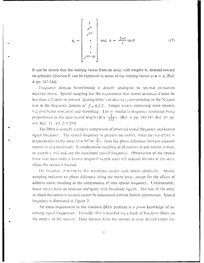
Sk= and k- 2d sinO 11
It can be shown that the steerinLe vector from an array with weights is, directed toward
anl arbitrary direction 0, can be expressed Ii terms, of thle steering vector as a = s. [ Ref.
4: pp. 3473-441.
F~requency. domain beamforming is direc:tly analogous to spectral estimlationl
decribed above. Spatial samlplig has the recquirement that sensor distances d' must be
less than A12 apart to prevent "grating lobes- (or aliausing: corresp onding, to the N\\quist
rate Ii thle frequency domain of' f,,, 1>-2 .Longer arra\ s. containlineL more sensors,
wIl I ive beter resolution a id smlo othingu. 'I his is Similar to F1req Uenc\ resolut ion betuc.1
proportional to the data record leng tli ( i Relf -4: pp.3141-34 5, Ref. 10: pp.
Th fe DOA is actually a reclative comparison of observ ed ;paitial Fr equency and known
Signal ft-c qucnev. *lhc spata frequency is Lireaze~t onl t'!h11c. wheni the v.wf ront is"
perpendic:ular to the arraty IU-900 or H~ ere the Phase difleren,.x between adja1cent
senlsors is at a nail u A slimlutai ieussmln of all sensors at onle instanit InI tim"Ie.
or, \ ip 111: wllldi,:itc thle mlaximium spatiatl filequencv,. Oboservation of' the spatil1
wave over titrie (with a known tenmpora I samplie ra-tec will Indicate the end of the airraLy
where the Source is located.
)n Orudsi 7' = o thI e wa l vfont xciCtes Cach senlsor iden tica Al. Spa-Ia
sampling11 indicates no phase difference along the entire array", except for the effkctS ofadditive noise, resulting Ii the computation of zero spatial frequency. Unfortunately.
hlnear arravs have an inherent ambieuiltv with broadside sienals. The side of the array
at which1 thle source IS located cannot he determined without further information. Spatial
11requencc Is i'llustrated InI Figure 31.
An extra requirement Ii the standard D)OA problem is a priori knowledge of inl-
coT'm:i eS e n1al [red uec:ies. T\ pically. thlis is h:! ml led \vIaI a bank of" ha; ilpa ss filters on
the output of thU ic eors. Data strecams fr-om the Sensors at each desired center FVe-

10
7.55
6 1,v I2
0~
-2
-4
-6-
a to 10 IS 0 25 0
ARRAY SENSOR7.5
Z5
S, -2.5
-5
-7.5
-10o ' ; i 5ARRAY SENSOR
Figure 3. Spatial Frequency: Two signals with SNR 2dB,
0, = lV and 0= 450 for two snapshots at time = (a) i0, (b,) i,. Notethe variation in 'DC level' as the snapshots sample the nearly broadside
signal at dill'erent phases.
12

quency J, ,. ... ) are processed in parallel, resulting in spatial frequencie. for each
temporal frequency. The DOAs are calculated by comparing these spatial frequencies
with the center frequencies of their respective filter banks.
Improvement in bearnforniing may be seen through the use of windows, weighing
each sensor output by the appropriate amount to narrow the bearnwidth or lower
sidelobes, but, as discussed earlier, at a cost of lowering overall resolution.
C. SUBSPACE METHODS
1. Introduction
The projection-type subspace method utilizes the properties of the
autocorrelation, covariance. or modified covariance data matrices and their
eigenvalue eigenvector decomposition into signal components and noise components in
eszinatine the DOA. Generally, subspace methods use an assumed propcrz\ of the data
to provide good resolution if the data fits the particular assumptions. cvcn for extrcie:i
short data sets. If the data (and signals) do not meet the assumptions. the result, can
be quite mislcaulne. The assumptions here call for white noise and a signal whose esti-
mated autocorrelation matrix converges to the true autocorrelation matrix as tie order
is increased.
For 1, comnIex sinusoids in additive complex white noise ta-c comnirned
autocorrelation function of the signal plus noise is given by
R1 I ?1 - 1~~r 4- 72otn
We dcine R-- as the signal autocorrelation matrix of rank 1. R:: = aI of full rank .l
anj ei';e the u1ocorrcatien matrix as
- ,ee. 1 + CI = Rs, ± R.h
where I is an .11by identitv matrix. R, is of full rank .A1 due to the noise contribution,
1) is the power of t!he itli complex sinusoid. cr- is the noise variance, and
e,[I .... c'- ] . tInfbrtunatelv. this decomposition is not possible \without
13

absolute knowledge of the noise. The p signal vectors e, contain the frequency infor-
mation and are related to the eigenvectors of R by v, - e, for i < p. The
eigendecomposition of R,, Is
PM
XX( + a ,)vjvif + ,v (20)
1= 1 i=p+i1
The principal eigenvectors of R_ are a function of both the signal and noise, If no signal
is present the autocorrelation matrix is simply a diagonal matrix with the eigenvalues
equal to the variance of the noise [Ref 1: pp. 422-423j:
2o 0(2 ). 0 0
0 ..R, 21)
o2
0 .
The data generated from taking .! samples of p sinusoids in white noise can be
used to Lencrate an autocorrelation matrix with the following properties:
* The theoretical autocorrelation matrix will be composed of a ,ignal autocorrelationnmatrix and a noise autocorrelation mcvtri'.
* lhe ,,nal autocorrelation matrix is not full rank if .l> r.0 The I? principal eicenvectors of the signal autocorrelation matrix may be used to
find the sinusoidal Frequencies.
* The p principal cicenvectors of the signal autocorrelation matrix are identical to thep principal eigenvectors of the total autocorrelation matrix.
The matrix will have a minimum eigenvalue / = o. [Ref. 1: pp. 422-44-11
Furthermore. the noise subspace eigenvectors are orthogonal to the signal
ei-envectors. or any linear combination of signal eigenvectors. [or the theoretical
autocorrelation matrix, R. all eigenvalues not associated with the signals are associated
with the noise and are identical in macnitude at , = . the minimum CiCenvalue of
R. Thus,
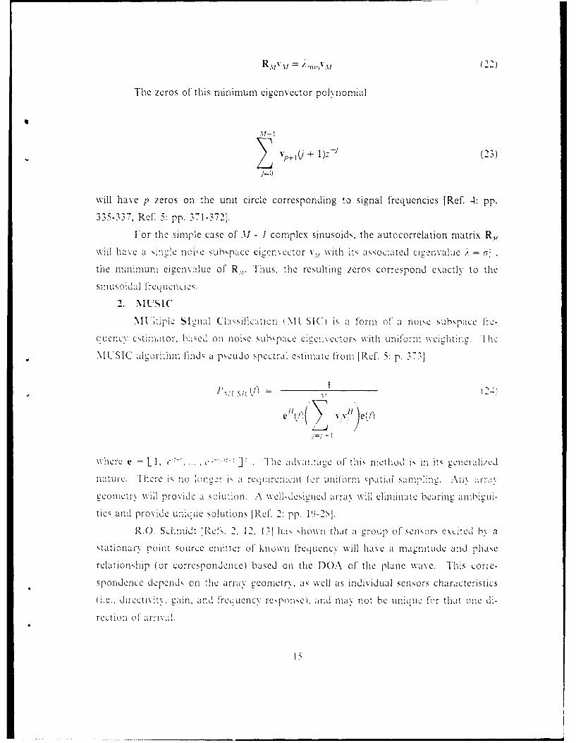
= (22)
The zeros of this ni~rmum cigenvector polynomial
Z ,, v~+ 1)7' (23)
wil ae p zeros on the unit circle corresponding to signal frequencies [Ref. .1: pp.
335-337, Ref' 5: pp. 371-372].
For the simple case of .1! - I complex sinusoids, the autocorrelation matrix Rfwil haC a s-InLeC 110"C subspaee eleenCrvector v, with its associated ciena7e , =a
the miinuni elgcenvaiue of R..,,. Thus, the resulting zeros correspond exactly to the
sinusoidal freqUenciles.
2. MUSIC
\1I~ipe ~calCla~i,,,f-cttion (NIt SIC) is a form of a noise Suhspac Irle-
q Uencv cbtaaCor hsclOn noise sU!bs'paC C;ge:nvectors with uiom ihin.I hic
MUSIC ai'-orithml finds a pseudo spectral estimate froml [RCe 5: p.3 1
where e E [I, c .c ' C-- "I Ileav~e of this method is in. its iLenerali/ed
nat oreC. Tfhere is no lonLeer i, a rec',1Iireme1)nt fr- Unif arn s patil smlig.:n am
Seon etlrv wil proVide aI Soluation. ellV1-desi Lenled a rra\ will1 elimlinate bea inei ambie (-ui
ties anid provide uniquLe solutions [Ref. 2: pp. 19~-2S[.
R.O. SLIhmlidt es.2. 12. 1 3] has showni that a group- of sensors eXcited h\ a
stationary point Source em-itter of' known f'requency will have at map iltude and phase
relationshIip (Or correspondence) based Onl the DOA of' the plane wave. Thi's corre-
spon-denice depends on thle array Ceometrv, as well as indiVidual sensors chara cter s tics
i.e.. dli ctivitv. gainl. and f'req kuenc% rc~ponse . and may not be unique for that one di-
rCtio o0 rr1 l
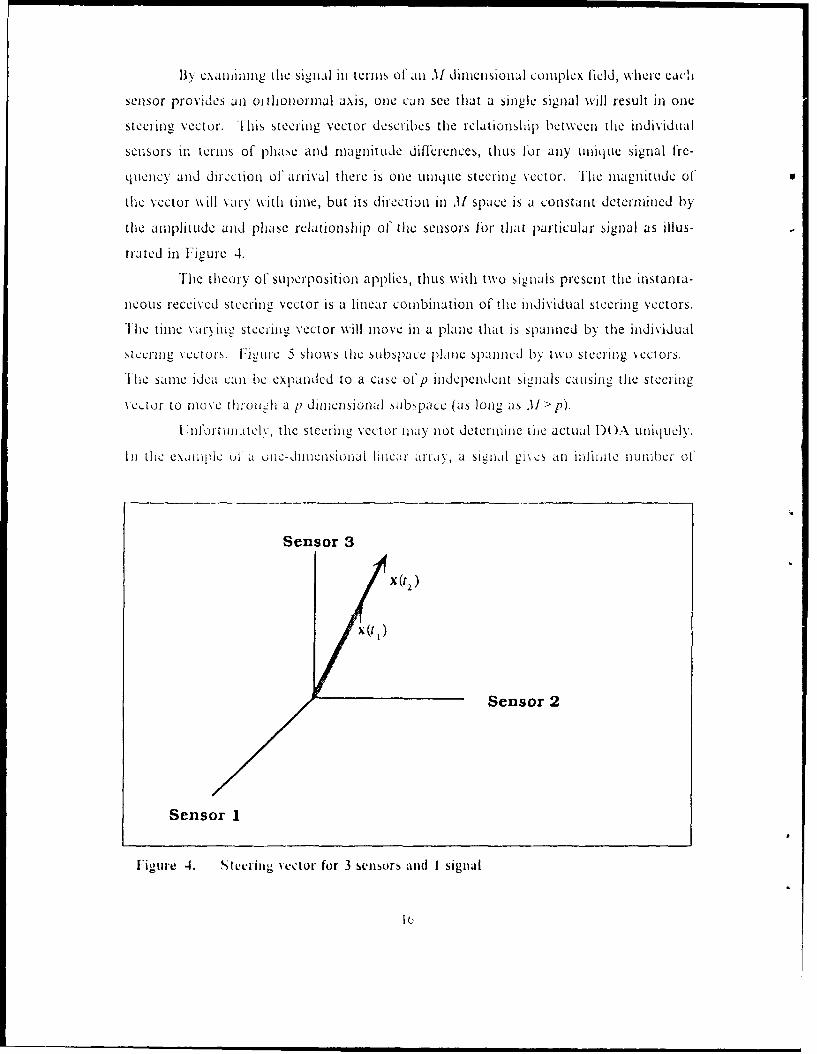
By exanjining the sienial in terms of aii .1l dimensional comIIpleX field, "-here eachi
Sensor provides an ozithonormnal axis, one canl see that a sinleI signal will result inl one
stcering vector. [his steering vector describes the relationship between the individual
sensors in termls of phase and magnitude differences, thus for any klliquLc signal fre-
quency and dircction of'arrival there is one unique steerig vct~or. The mlagnlitude Of
the vector m\ill vary with time, but its direction in .11 space is a constant determined by
the dinlphit tde and phase relationship of tI ie sensors for that particular signal as ilius-
tra td inl Figure 4.
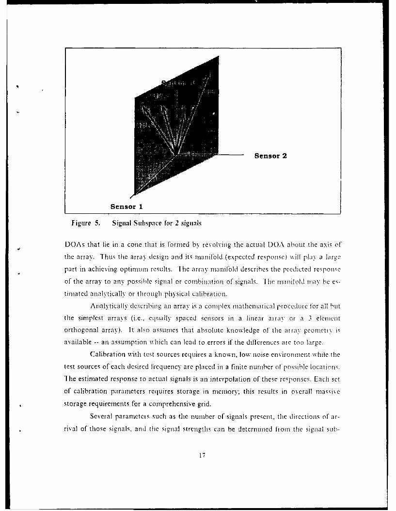
'Fhe theory of superposition applies, thus With two signials present the instanta-
neous received sieeriie vector is a linear combination of the individual steering vectors.
The time varving steerinc, vector "T'i ove in a plane Mha is spanned by the individual
stccring Vct~ors. figure 5 Show the snbbpac p~lan~e spannedI by tWO steer-ing vectors.
'ile Samle idea can be expanded to a case ofpq independent signals causing the steering
NCtor to mov110roiJ a 11 dimensional sub~pace (as long(- as 11>p).
L nfi t inaitely- the steering vector m'iy not determnine tile actual DO( A uniquely.
In [tie example of a unc-dincnisional linear ara a signal gim c an infinite number of'
Sensor 3
x0(2)
xQJ
Sensor 2
Sensor 1
Figure 4. Stecring 'ector for 3 Sensors anmd I signal
lo
Sensor 2
Sensor 1
Figure 5. Signal Subspace for 2 signals
DOAs that lie in a cone that is formed by revolving the actual DOA about the axis of
the array. Thus the array design and its manifold (expected response) wxiII play a large
part in achieving optimum results. lhe array manifold describes the pi cdicted responc
of the array to any possible signal or combination of signals. I hemanilold may be C-
timated analyticallv or through physical calibration.
Analytically describing an array is a complex mathematical procedure for all but
the simplest arrays (i.e., equally spaced sensors in a linear atray or a 3 element
orthogonal array). It also assumes that absolute knowledge of the atray geomett. i
available -- an assumption which can lead to errors if the differences are too large.
Calibration with test sources requires a known, low noise environment while the
test sources of each desired frequency are placed in a finite number of possible locations.
The estimated response to actual signals is an interpolation of these responscs. Each set
of calibration parameters requires storage in memory; this results in overall massive
storage requirements for a comprehensive grid.
Several parameters such as the number of signals present, the directions of ar-
rival of those signals, and the signal strengths can be determined from the signal sub-
17

space inflormnation. MN'ore complex models. hoxwever. can be develope th can
determine signal frequency and polarization as descibed in References 2 and IS1.
We will now describe the basic steps in the MULSIC algorithmn f ,or the D)OA
problem. First. we sample the signals and compute the autocorreiation matrix of- the
data R. Then. we determine the ordered set of cicenvalues arid cicenvectors of R. In
particular, the cipcenvectors associated with the minimum ejeenvalues must be accurate.
In thle theoretical case the siznal ci en values are composed of signal strength (P, ) and
noise variance ((72 and the nonprincipal eigenvalues will all be identically c.
We now determ-ine the number of- sigenal by eicnvalue comparison. A siple
counting of the eigenvalues greater than 72 wvill give the number of signals present in the
theoretical case. IHowever, the samiple autocorrelation. estimates does not lead to such
simple results. Small power level signaIWI 11 hlave Small CILenvalu eS (perha 1T- STmaller
thanI r" . and the, no: iCe a e w ill no(t acItuaLl be idetcI[ ut J wilCL eop or cluster
near an approvimation of' c,: NI ethu1ds, o! ou in iClUde likelih ood ratio te,,t, wheLre
thle canis bctwkc'I til. ecvle deternI"I::Q threshuld Placcnlt jRef2:pp jT
Onice -xc 1i mU ti, 1;e i mber of iaI -preCen We Liln 2ete-,Lrrine tles-c d sn
Co' ioU : *e: 1 ersec: oft1I %spa 1 it the trra% malcnifoUld. 'I he
FWO aJCI are\Of U ~ the NI L SI C al co:1thi hmlirc theC calc:u!lation andstoraceI, T1 tI" aI Ia' nIma an rIo th 1 uenaC..oIp !\:Ilen 0l1th
Li Lt OLOrreillt:011 nil:tr1-; thaLt resui!ts ham er jhtr-Cc allra S.
3. ESPRIT
InI Re eQrenc 14. Paiulraij. Ru%. and K ailath decieEstinlutiOn Of Si l-'1
Pau~er .a a~:oa ~vai:;eTcI.,tcsI.I~IIK tb~'e:nt~lNx..

separates the two parallel su!barrav's. but no rotation can be presen- Each sensor inl a
matching pair (doublet must be ientica!. but knowledoc of individuail sensor and array
response characteristics, is not required.
The A' elements of both arrays arc sampled simul taneou ly "ith the signal at
each senSor bein.a gi% -n byP
XPr) = SPAt)O;(k) ± ,(1
(27)
whee te sn~~aJQrtlat kedch venmor in a doublet difnds only h; a phase termin
additive noise NOti t'sQna I present. sis the wavefront at the reference senlsor inl The
X arra LH , DOA ') reh : aC to Trae Ldi pla ,Cnamait ctraU.is the respons e (.1 dic
Sthsj~arinllN ara ralat ,i \ to the r f-erece sen sor in that: a:rrax fora si !IYrn
baa in a . I ar'C a i d of theI di spiaceman clt sect i and n the n c)i' Na t ar. Il %evctoar
:atra.:aas~a a i s ' O: SLII'rax is arc:
X I/) = S(I) -T 1i'
x ' L x: (, x, f1) x.,! W
lhe cwor of w~ax ~rot at the refrence sensc:r in array N is represenlted b\ s/i). APl
di N~hj ar a:1 ,1p as diIlarece~S are based oin ths sen or. The r by p diaaoma I w-
tri \ (I). ol1a1ir.N tL hwtas dela s that ccc or with each, Set Of' douablet s
are s~ . s sr\\n ill cqjatiort I-I

if R., is the sienial autocorrelation matrix, the subarrav autocorreclation mnatrix
is cive bIA
IT
I-le cross correlation between subarravs is
Rx. HR (D 7 H (3T
where H is the direction matrix whose colunrns are thc direction vectors for thle p
Nvave!front s
hI 9;.) = hC).h, 0k). h,,,O) ] T33
A\lter Some nwampu!Latlon j Ref. 15:; pp. 2>1 -25'31],\we obtain the matrix
HI PT - -/(I J-4)
1: cvr there- wvill be p cigecnvalucs of this- matrix. But wlicil c .tile it h row
I 1' CLOmIcs Iero. leavine, r-I ielaas achJ value of', where this occ .Ur\
cjid ace~cla/LX ei22 OUC(Cl).Nov. the Do:\s can he determnIled hx
Dlie to e\timatloni errors InI thle callttionI Of' thle correlation matruLCs. SOme'
err-or wil! he inldu Cd. Genecrally, the GF's will be moved oil' the uit cir-cle and out from
he-. o1- ut- in theC ca~c of' ;iron u sena I .thyWill Still be Ca si1 diLCernibieC. It sI 1o Ld1
be notedj thltt poor arrax dcSlugn may result InI possible aimbi gities (similar to \Mt~ SIC).
Adx ntaecsto note, o'e(r the NII SI C ahleorith come with respect to the arrty
nunilb11"ld. \ith I S P RI V. no manifold is required. The considerable calibration elfforts
a~d~trk2 rc,;urement, are nonexistent. I [owc\ er. the two subarrzivs nmist be, identic il
In .irIlctd 1-C sth o \it ioned evlctlv rar-allel to eachl other r[Ref. 1V.

4. Other Subspace Methods
Larze variance effects may bc seen in the abo~e method" due to the poor reli-
ability of' the estimation of the eigenvectors associated With the minim M I~ealueCS
of the estimated autocorrelation miatrix R, A dillerent method of' spectral estimation
is the use of the principal components where only the cigenvectors associated with the
Iargest ei genalues are used. Somec methods have tried to niinim i/e the efct foic
by using R,~ - a~I but the estimation errors in both R_, and C2 have limited their suIc-
cess [Ref. 1: pp. 4251. Other spatial spectral methods include the parametric methods
Such as AR and MN/L [Ref. 1: pp. 426-4271.
The structured matrix approximation of Kumnaresan and Shaw IRef. 16] uses K
sna.1pshots in time of an NV element uniformldy spaced linear array with each snapshot InI
time forineri a colunmn of, a data matrix X. whi,11h is then approximated by X, in the least
sq uares sense. The bcaringz Iinformation, Is then calculated u '1"in the prpisof- the
Vanderm~onde matrix.
A combination of frequency domain bca~nrorming and autoreeressive moodlne:
techniques have becen employed in Referience 17 to estlnute the direction of' uri l In,' a
mu11tTil Source localiz'1atl'1 ion10 situatio Us~ a pIlnar ar
lfi aipenv and Childers, lRef. 1 SIl usc 1c icv-a\nnerftrsto -,cak he
multiple wave case dov.-n to a succession of single wave problems.
Reference 19 q explns an ai-o rithm tha-t uscs n oni-inoi c cicen scct ors f'roml a1
cova riance matrix to obtailn hi Lh rcsol ution diircction of arrival for narrow bandJ sources,.
An ada ivc eanoni methoad sine br to a mini mum energy- a pproac.h is;
dzcibc inRe!tI1cc 20. *Vc C'-ntuc r of' the correlaition mIarix ian'cdand
the conipat t osaCnodlicd to orPtimi/C resolotionl but at a cost of array 1:ain!.

III. THE LANCZOS ALGORITHM
Lanc7os algorithms provide a method to find some of the extreme eigenvalues(smallest or largest) and their associated eigenvectors from large matrices with fewer
operations than required in an entire matrix decomposition. The procedure is a
tridiagonalization of the original matrix based on an iteration developed by Cornelius
Lanczos [Ref. 21: pp. 49-206]. Once the matrix is in a tridiagonalized form the
eigenvalues can be easily computed using a symmetric QR algorithm [Ref. 15: pp.
27S-279] or bisection (with or without Sturm sequencing) [Ref. 15: pp. 305--SS]. lhe
algorithm takes advantage of "mininized iterations" providing quick convergence to the
final tridiagonal matrix and avoiding accumulation of roundoft error. [Ref. 221
The method fell from favor as a tridiagonalization technique with the advent of the
Givens and Ilouscholder transformations later on in the 1950s. Giveis transfornacions
[Ref. 15: pp. 38--47] use plane rotations (orthogonal matrices) to zero out u, desired en-
tries in tht matrix undergoinig tridiagonalization. The H ouseholder methods Rcl . 15:
pp. 43-4-1 use elementary reflectors to accomplish the samc end. Both methods are in-
herentlv stable, with the H ouseholder method being slightly superior in both speed and
accuracy. Both methods outperformed Lanczos as a complete tridiagonalizati on proce-
dure in the general case \where all eigenvalucs are required [Ref. 23: pp. 42-431].
The real po-x Lr of the Lanczos method however lies in obtaining the extreme vluLcS
quickly. lhe entire natrix need not be tridiagonalized before solutions start to converge.
Also. ifthe ori" al natrix is sparse, the Lanczos method maintains that properti. sav-
ing even more computations. - hus for large matrices (order 1 00i) the I.anczos methodwill converge on extreme cigenvalucs in many IV wer operations. Recently -I uft and
Nlelissinos [Rcf. -24: pp. 43-4-17 have derived a variation of'the Lanczos mehod for high
resolution spectral estimation and showed that their method outperforms both the sin-
gular value decomposition and the power method of principal eigenvector and
cigenvalue computation. Later in this chapter, it will be shown that storage require-
ments are also minimized.
Ihis chapter starts with an explanation of the classical Lanczos algorithm as devel-
oped b Lanczos and modified by Paige Ke" 25]. Then we will discuss the unorthodox
l.a ucZos algeorithI of Cullur and Willoughbv where no reorthogonalization i; per-
formcd [PReV 231. -irialy. the algorithii used in the direction of arrival problem are
22"

discussed in detail. Also, we present sorne results of the algorithm in the form of spectral
estimation of multiple tones.
A. CLASSICAL LANCZOS AND ITS VARIANTS
The original algorithm was designed as a means to directly tridiagonalize the sym-
metric matrix A. The development of Lanczos algorithm requires the knowledge of
Krylov sequences and subspaces. For an n by n matrix A and any arbitrary non-null
n by 1 vector v, the Krvlov sequence of vectors is defined as:
Vi+ 1 = Avi = AIV, for k = 1, 2, .. n (36)
In the above sequence there will be a vector, say v., which can be expressed as a
linear combination of all the preceding vectors. The Kr-iov matrix of rank m ik then
Zi en by
,,= [v V . ,] -- 3. Av . A ' (7"
and th~e Krylov subspace is the space that spar's Zile vectors Iv:, I..,
K"'>A. :I--- .,pan [v , Av:, Aav: . A:*- * (3\
The columus of the n by m Krvlov matrix \ are orthogonal. lhe tridiagonadi/azion
of the ,:iven nuatrix A is then obtained as
T=V.A 39)
where T is an ib in tridiagonal matrix. Thus. the givyen matrix A can be
tridiagonaI"zed provided we have an elicient wvaV to compute the orthoconal matrix V.,
or to compute the ccnicnts of matrix T by performing the decomposition of e ation
39 directly as proposed by I-anczos [Ref. 22, Ref 15J.
The most direct way of perfornng the tridiagonalization assumes that T = V'AN'
where V = [v, v, ... v,] . Note that A is a symmetric n by ?, matrix and V is an
n by in orthogonal matrix constructed from the krvlov ScqLuence of vectors. The basic
recursion for a real n by n mat2: A starts with a randomly cenerated unit Lanczos vec-
tor v1. Define scalar / = 0 and N, = 0. Define Lanc.zos vectors v and clements - and
P/ - for I = 1.2 ... , 11,
f!.:V 1 --- A N: - ,Ti'i - i'_ d

T
v ,-Av 41
This is referred to as the basic Lanczos iteration or recursion. The actual Lancios maj-
trix T,, j = 1, 2, , Af. is a symmetric tridiagonal matrix with o., ,1 i <j, on the di-
agonal, and ,1 5 1 cj 1), above and below the diagonal.
0 0~Jj
Fach new Lanczos vector A-- is obtained from orthogonalizinc the vector Av, with
V, and v, Thel elemnents Y., and P) - are the scalar coemlcients, thatt nmake uip the fatnc/os
miatrix. The basic Lanczos recursion mnay be conidensed into mnatrix notation by dtefInIne
(V;V, ,v-). T hen f romi equations -40. 4 1, and 42
where e, is the coordinate vector whose uith component is 1 wvhile the rest of the comi-
ponents are ), T, is the ni b% in Laniczos matrix, the diagonal entries arc
T,r iA k Fo fr I ! A n(45)
and the entries along the two sub-diaco-.nals on either side of the principal diagonal are
Tn(~ )= T_ Ak +- l.k) =-k+l for I k-m n - 1(4w~
Note that A is never modified (unlike in Givens and H ouseholder trailsformiations), thus
advantage max- be takeni of any,, existing sparsity. Also, thle only storag requirements
are for the three Lanczos vectors (n dimension), the Lanczos matrix T.. and the original
matrix A.
We summlarize thle actual Steps:
SUse the basic. recuLrsion Of, equationIs 40. 41. and 42 to translbrmn the ',,nmnetricmnatrix A into( a finiijv of synimeti ic tridia-onal marcsT L" 1.I

" For in .1/ Pod the eigenvalues of T,. u (also known as the Ritz values of T,).
* U..se some or all of these eigcnva lues., p. aq approximations of the eigen'values ofA;.
" For each eigenvalue u find a unit cigenvector u so that Tmu =p
The Ritz vector A, is the approximation of the eigenvector of A. It is found from map-
ping the eigenvector u of the Lanczos matrix.
N. - VM U (47)
So the eigendecomposition of T. finially results in the Ritz pair (gi, y) which approxi-
mates the cicenvalucs and eieenvectors of A. [Ref. 23: pp. 32-33., Ref. 15: pp. 322-325-1
Unfortunately, the effects of finite precision arithmetic prevent the theoretical
LanTc7oS alcori1thml fromn working. The cigenivalues of A and the ecenv alues of T_~ no
lanLcer converge. Roundoff errors are partially to blamne, but the dominant effect is From
the loss of orthogonialitv of the Lanczos vectors v F Vro m equation 40 it can be seenI
that a small will have great effect on Plaice showed that the algorithm run1s
witinallwaleerror constraints until It stalrts to coIIveree Onl the first ciLen\ lu1C. A\t
this point § bccemcs smll1 and the Laniczos vectors lose orthioeonahtv-. The loss of'
orthogonalitv Is niot random,. however. It alwavs occurs in the direction of' the Ritz
vctor V.
Th IS tr'oable can be dealt with through rcortliogoralization. But questions tha t we
mlust anlswer inlLue:
11O I ow mch roiaaonlitinis req ui rcJ?
*Where shouldd it be peifrcaed
* Rc :t cooiia ,\ with r-C"Fcct to vn ht?
Coinplete ,crj~f~a:amlis the first choice, inserting a HIouseholder matrix
compauta non Into the Lalnc/o J-- orithmn. This en~fbrces orthovona lity amoing A the
Lanicios vectors and is el"Luc iat keeping the sy stem stable. But the extra comniputa-
tions it requi.1res nIC2euc Mill aldvantase of the Lanczos, alieorithn-. makinec the numbeihr of'
computationls on) the samne or-dcr as ai complete decomposition. Numerous vectors have
to be stored and conioa red r equirilhe man111 swaps), into and out of' storage. I Ref. 15: pp.

Selective reorthogonalization is clearly more efficient. The extra computations are
performed only it orthogonality checks indicate loss is imminent. Paige shows that the
loss of orthogonality occurs only when the algorithm converges on a Rit/ pair. Thus,
instead of reorthogonalizing against every other Lanczos vector, using the less numerous
Ritz vectors will be sufficient. Storage is therefore ninimized. Only when all eigenvalucs
of the matrix are required does this method become computationally more expensive
than other techniques. [Ref. 26]
The last option is no reorthogonalization. The explanation above would seem to in-
dicate that maintaining orthogonality is required. However by analyzing the causes and
effects of the original loss of orthogonalization one can insert corrections into the sol-
ution to give valid eigenvalues and eigenvectors. This is the procedure that will be ex-
anuned in the next section.
One other property will be mentioned. lere the single vector Lanczos recursion
described above will not lind duplicate eigenvalues of the matrix A. Parlett's proof uses
the power method to expand v to compute the columns of the Krvlov matrix K'(v. A).
If 1(v) is the smallest invariant subspace oF P. which contains N. then the projection of
A onto J(v) has simple eigenvalues. Also, the Krylov subspaces fill up 1(v and for
some / < n we have
sptv,} a K21A, v) c A"(A, v) c ... c KI(A. v) = K1+ '(A. v) = f(v) (-IS)
The reult is that sonic eicenvectors of A may be nissed, and anm repeated ejgenvalucswill not be detected. [Ref 27: pp. 235-239]
The multiple eigenvalue problem can be treated by using a Block Lancz:s algorithm.
Instead of obtalliHiL a tridianonal matrix, the result is a banded block matrix, where the
diagonal is N1. an I by I matrix, and the above and below the principal diagonal are
upper triangular matrices B, . Lach block must be dimensioned I > p . where is the
estimated multiplicity of the desired eigenvalue.
MI T2 0B, 1 2 B, 0
0 B3 0 9
0 . ,. B0 u0 B1 NI)
26,

This is analogous to the general case [Ref 15: pp. 337-3391. The block Lanczos alpo-
rithm is briefly reviewed at the end of this chapter.
The above discussion assumes that the given matrix A is real and symmetric. Besides
the algorithms sumnmarized in this section for a real and syinmetric matrix case. there
are other general Lanczos algorithms proposed in the literature [Ref. 231 that are suitable
for Hermitian matrices, non-symmetric matrices, and for rectangular matrices.
B. IMPLEMENTATION
The Lanczos phenomenon states that a few, not all, of the eigenvalues of a very
large matrix A can be computed using the Lanczos recursic- -,ith no
reorthogonalization. But to find most of the eigenvaiues, the Lainc7os matrix, T, will
grow in size approaching that of A. causing the loss of orthogonality of the Lanczos
vectors. TIhe loss of orthogonalitv results in many spurious eigen alues. as well as extra
copies of good eigenvalues. In any case, a test is required to confirm either:
* a "found" eigenvalue is good, or
* the cigervalue that appears is spurious.
Golub and Van Loan. Parlett. and Paige [Refs. 15. 27. and 28[ describe Procdures
that look a.t the eiecnvalues for each T. as n is stepped up in size. All the eigenvalues
ofT.. ,re computed at each step. The good eigenvalues will repeat at each larger T.,
while th e purious: ecuxalues jump around. If an eigenvalue does not match at con-
seTe',e is it mve cons idered spurious and thrown out. If a good eigecnvalue is
... , e due to numerical roundolf), it can be counted on to reappear in the
.. . Rf.2! tuke a dil]erent tack by developin,, a test to find
and eliminatc bad eigciivalues and retain the rest. The advantage here is in utilizing the
machines tleran.ce to dr , Lid ejuenvalucs. while not discarding cood ejieenvalues that
Live vet to cow cree...\ ' a result a larger spectrum is available sooner, even though it
my 0a1x be a rouc:h etimate of where the cigenvalues will finally converge.
1;.pr e. p,,rts of the Lanc/os recursion (equations 41 and -42) are replaced by
Yi= V1i4.- lv,
and
fi = Al.v-z',v, - /; v,: (51)
01N*
Computation of the element Lx, is a modified Gram-Schmidt orthogonalization proce-dure. The new fi,-, is equivalent to the - of equation 42 but now it directly controls
the size of the Lanczos vector.
In what follows we describe two Lanczos algorithms, namely the single vector
Lanczos algorithm which is modified and analyzed by Paige [Ref. 281 and the block
Lanczos algorithm described by Cullum and Willoughby [Ref. 23]. Both algorithms have
been considered for the estimation of the directions-of-arrival of multiple targets in noisy
environments in this thesis.
1. Single Vector Lanczos Algorithm
The first procedure to be described is the Paige's single vector Lanczos algo-
rithin jRef. 20 fcr real symmetric matrices. The single vector Lanczos procedure is one
of the most straightforward implementations of the theory. This procedure will find
sonic or many of the eigenvalucs and eigenvectors of a real synnetric matrix A such that
Ax = /x. It will not detect repeated eigenvalues. I lowever. it may be noted that for
many problems of" interest in practice we do not have strictly multipic cigcenvalues. [or
example. in the direction-of-arrival problems the smallest eigenvalueq of the
autocorrelation matrix corresponding to the noise associated with the target signals are
sprcad over a small rance rather than coinciding on the same value [Ref. 21.
No reorthogonalization is performed as part of the single vector Lanczos al-
gorithm. As mentioned earlier, the lanczos vectors becin to lose their orthoeonality
when we cck to estimate all or most of the cigenvalues of the real sxnimetric matrix A.
[or the appilcationl under consideration, however, we are generally interested in only a
fcw of the ncnimu rienvalucs and the corresponding cicenvectors. It is mainly for this
reason that w c have not attempted the complete or selective reorthogonalization of the
Lanczos vcctors in this study.
Now we shall outline the basic steps involved in the sine 'c ector LIane/os al-
gorilim. -I his is based on the recursion described by equations -40, 50 , aid 51. Bascd on
these equations Paige [Ref. 28] presented four different single vector algorithms. We
have adapted one of in this study. Ihe complete cigenvalue cigenvector problem actually
consists of three parts: (a) obtaining the tridiagonal matrix T. from the given symmetric
and real matrix A using Paige's recursion, (b) determining the smallest eigenvalues of
T-. using tile bisection method and Sturm sequencing, and (c) estimating the corre-
sponding cigcnvcctors by coMputing the Ritz vectors. The details are presented in the
f, lo \v iL.
2S

Step 1: As shown in equation 43 the smnietric tridiagonal matrix T has entries
a, and P3 along its principal, and the adjacent sub and super diagonals, respectively. The
Following recursive expressions are then used to compute the entries of the tridiagonal
matrix, and also the Lanczos vectors %, lRefl 2S]:
Initial conditions: v1 is an arbitrary n by I vector such that 11v112 =1
U1 = Av 1
a = 0 = 0
forj = 1,2,...,m
V I )I /"/hi = U. -11
I'+] = vj'~
1/+i =Avi+1 - PAi
where w. and tl are some intermediate vectors. The vector v, is obtained by filling its
entries with a random number sequence and then normali1in it with respect to its
Euciidean norm. Now T... is obtained , simp!y fillimg its entries as in equation 43. Note
that m < n in the above. One quick test to ensure that we have obtained a fairly accurate
estimate ofT is to compute the product v,, . The result should be equal to ; .where
is the Kronccker delta function.
Step 2: The eigenvalues of the tridiagonal matrix T-. denoted by si.. can be
computed using the bisection method and Sturm sequencing. Actually one could obtain
both ci :en, C ilues and cicenvectors of T, by employing such methods as the QR algo-
rithm. I low ever. when onlx a few eigenvalues are required. the bisection method seems
appropr-a c. I-or the given m by in matrix T. we define the characterstic po nom ial
p?,.u,) = det (T, - p1) (53.
which can be rccursively con Mputed as follows
P =
P (p) = -t:,) = -_,u)try-.(uL) _ fi _l, fs ) (4
for = I.
2()

The roots of the polynomial p.(,u) are the required eigenvalues. For our appli-
cation, we are only interested in a small range of eigenvalues at the lowest end of the
eigenvalue spectrum. We make use of the Sturm sequencing property that the
eigenvalues of T,, strictly separate those of T, [Ref. 15: pp. 305-3071 and implement the
following iteration:
a+ha- 4-2
b if r,(a)p,(h) < 0 (55)
a u if jm(a)p,(b) > 0
and we repeat the above as long as b - a > c(I b +a ), where F is the miachine
unit round-off error and [ab] is the range of our required eigenvalues. I)eterming- the
range of interest in our application may require some a priori knowledge about the signal
to noise ratios (SNR) and it may take a couple of iterations to do this. Some alternatives
to the iteration ev en in equation 55 are to use a strtiehtfor,.ard polynomial root lcr
and then pick the roots of interest, or to employ the well known L-D- I facterization.
both of' which ma'. not be computationatly eflficicnt.
Step 3: There are two ways to obtain the eicenvectors of A knowino its
eigenvalues. .Note that U. are the estimates of/.. In the first method, we compute
the eigenvectors of .' denoted b t. and then obtain theeicenvectors of A given by
x. = L,4 .(,
where L, = Ev- v, -v is the Lanc/os matrix which ideally is the sa.ne zs the
Krylov matrix of equation 37. Note tha:. t eT-
IThe second mCthod invole: compu t ing the Ritz vectors cit her "rum the
Rayleigh quotient interation or by the orthogonal iteration. I lere we assume tiat we
have good etimates of/" from the previous step, and proceed to obtain the eigcnvector
x by mininizing the cost function
J = !.(A- )1)xf: (5
It can be shown that a simple miniization of J with respect to x yields the R leigh
quotient ofx
30

xA-xr(x) j 7' (S
Therefore, given ,and using equation 5S we can formulate the Rayleigh quo-
tient iteration as follows 1 Refl 15. 27]
Initial condition: x,) is an arbitrary vector such that IXGI!= I
fork = 0) 1,2..
x T~ Ax,
solve (A - rN~I k for %-.
X,.
where N-,, Is somec intermediate vector. W\e stop the iteration when v _converees to
a conl<amt or when ;-A, ) one of01 the knlown1 e-CMna dLiCe At eaCh iteratiostpw
needU to SolveC an. 17 1-,%/ emStc of equations inI this method. One atdvantaee w th tI
method, however, is that it converges very quickly. Besides the above iteration., someiothr m t ciar oa lnedin efrenesI ~23and 27. We remark thtifoii' a leW
ecenvltiesand ccvecors isay. five' are required. it max~ bie miore dircet : to lO\c
We n ov.' pr eCent an exa mple of the a bility of the single vc:tor nci /os a rrm
to CesHi1-C Te th drct on ef ariaor to find spectral l:ies I noise. and thead m:e
in IIe\trac~lin- more1- thanl onle ci1n11ead ejenvecOr' Inl this proceS. WC LoIdr
V~n ith Three si:Uso ia\peeti o
A'! 1; cos(27f;n) nn
w here A, are the amplitudtc, of sinusoids. f are the normalized spatiail frlwecies
0). corrc-mid ing to ZI() ? 'I n (el o s theC zero mlean1 white-, no(ise withj
al valrlince of -n

We have computed a 25 by 25 autocorrelation matrix of x(n), R,, , by using 100
data samples. We have used the covariance method for this purpose, hence R,, is real
and symmetric. The eigenvectors x, of R,, corresponding to the lowest eigenvalues are
computed by employing the single vector Lanczos algorithm. The power spectral density
estimates are computed as follows:2
s 2- (61)
Z jiz 2 = gfl/1=0
where x,, are the elements of the jth eigenvector, xj.
Figure 6 and Figure 7 show the power spectral density (PSD) estimates of
equation 60 with an SNR of 10 dB forj = I and 2, respectively.
100
to-
M 10-2
10-3 A
CL
-4
05
0 20 40 60 80 oo
Bearings
Figure 6. PSD of first eigenvector
Note that the index j indicates the increasing magnitude of the eigenvalues. Thus,
(., x,) are the lowest eigenvalue and the corresponding eigenvector. In both figures we
have the peaks at the correct locations (90, 27, 630). However, they both have spurious
32

smaller peaks at different locations. We can observe the same trend for the first five
eigenvectors as shown in Figure 8, where the spectral estimates are over laid on each
other.
Based on the above results one feels that we could employ scme kind of aver-
aging to get rid of the spurious peaks and improve the estimation performance. We have
implemented two such methods: the eigenvector averaging and the spectral averaging.
Figure 9 shows the result of the algebraic averaging of the first 5 eigenvectors, and
Figure 10 showb the result of the algebraic averaging of the spectral estimates of the
same eigenvectors. As secn from Figures 9 and 10, eigenvector averaging yields better
results than spectral averaging.
100 7~
10-i2
7.
10-1'
1 0 _ _ . . . . - -
0 20 40 60 80 1o0
Figure 7. PSD of second eigenvector
Improved results, however, were obtained by using what is called spectral
multiplication which is obtained by taking the product of the individual spectra, given
by
J
0 I SOO(62)
j=1
33

where J is a predetermined number (J < in < i1). Figures II and 12 show the results of
spectral multiplication for J = 2 and J = 5 , respectively. As can be seen in these fig-
ures, using more spectra in equation 62 greatly improves the performance. Also. even
for J = 2, spectral multiplication outperforms the eigenvector averaging method.
100
S10-2
5,
10-1
CL
10-.
10 -
iO-S _ ____
0 20 40 60 on 100
Rea rirlgq
Figure 8. Oierlayed PSDs of first 5 eigenvector
In the remainder of the thesis, we have used spectral multiplication in prefer-
ence to the eigenvector or spectral averaging. Figure 13 shows the multiplicatiun of 5
spectra for the case when the SNR = 0 d0. We notice a spurious peak around
0 = 74'. More spurious peaks are observed when the SNR is decreased to -5 dlI (see
Figure 14) and Figure 15 shows the spectrum for the SNR but we have used the
eigenvectors 6-10 in this case. Improved performance is obtained as shown in
Figure 16 (J = 10) and Figure 17 (J = 15) by using more and more eigenvectors in the
spectral multiplication.
In all the above cases we always observed the signal spectral peaks at the right
places. The spurious peaks, however, did not appear at the same location as we used a
different eigenvector to compute the spectrum, Sc,(f).
34

100
10-4
0 20 40 60 80 10
Dearings
Figure 9. Eigem ector averaging
10--
I..
0
CL
10-4
10-50 20 40 60 80 00
Bearings
Figure 10. Spectral averaging
35
200

100
20-2
StO-i10-3
,,.€. 10-4
10- 1
0 1040- 7 1o
C-)
09
1 0-0 in
Figure 11. Spectral product for 2 eigemectors..
00
e0-;
10 . 2 4
L0 20 40 60 80 100
Bearings
Figure 12. Spectral product for 5 eigenvectors
36

10-I
10-2
10-3
1 0-4
-6
0-7CL
, 0-8- 9
LC-
0 20 40 60 60 100
B3earingsa
Figure 13. Spectral product for 5 eigenvectors, 0 dB
10-2
1 0-3C
1 0-'
1. 0-6
CL,
06
1I 0-9
o10-10
0 20 40 60 80 100
Bearings
Figure 14. Spectral product for 5 eigenvectors, -5 dB: Using second through siXth
cigenvectors
37

10-t
10-2
S10-4
-,10-6
C)10-8
1008
1 0 -ia
00
6 0-I
10-5
10-6
CL
S10-'
1 0 -9
Cl 20 4000-0 10
1038

100
to-o
iO-6
10-7
I0-6
U
I.
OV
I.I O-v
0-
t0-1o_ , I ,,
0 20 40 60 80 100
Bearin
Figure 17. Spectral product for 15 eigenvectors, -5 dB
2. Other Methods
ihe single vector Lanczos algorithm will not determine that repeating
eigecnvalues exist, thus it cannot find the corresponding eigenvectors. lie subspace that
results has an incomplete basis as it is described only by the eigenvectors that are com-
puted. The 6ulution is to use a bloc'. -nethod that is analogous to the single vector
Lanczos algorithm. As we mentioned earlier, the block form of the Lanczos algorithm
does find eigenvectors with multiplicity p as long as the blocks are dimensioned I > r.
We attempted to incorporate the Cullum and Willoughby hybrid block Lanczos algo-
rithm (Ref. 29 Chapter 8) into our direction of arrival model. We postulated that it
would be desirable to compute a few of the extreme smallest repeating cigenvalues and
their respective eigenvectors. I Iowever we were never able to get the program to reliably
compute good eigenvalues and eigenvectors for the autocorrelation matrix. Tlhis has not
posed a problem for our model as the covariance matrix does not appear to have re-
peating eigenvalues, but a larger order matrix may indeed include duplicating noise
cigenvalues and require an algorithm that will accurately operate with that perturbation.
39

The algorithm we attempted to use is actually a hybrid approach to finding the
eigenvalues and eigenvectors of a real synmmetric matrix A. For insight into the problem
look at the block analogy of equations 40, 41, and 42. Define matriccs
B, 0 and V, -- 0. The n byq matrix V, has columns that are orthonormal random
vectors. The value of q must be greater than or equal to the number of eigenvalues to
be found.
for i= 2,3, ... ,s
=+Bi+i Pi = AV - \AMi- Bl (63)
Ni V_ T (AV - V11 B1i) (64)
The matrix B, is a modified Gram-Schnidt orthonormalijation of the columns of P,.
Also note that the matrix NI correspond to the :s of the single vector Lanczos.
t he block analogy to the Krylov subspacc approach cain be performed with
K (A. V') s n ~V 1, AV , A 2, .. A -'V}N~ (66)
The blocks V . for j = 1. 2. s form the orthonormal basis of the Krylov subspace.
It can be shown that for a symmetric n byn matrix A and an orthonormal
?, by/ st.tine matrix Vi. that the block recursion equations 63, 64. and 65 will gencrate
blocks V:. V3. , V where qs < n. It is these blocks that form an orthonormal bass
oa the subspace K A. V). In much the same wav as the single vector Lanczos aioorit" "
eneratres the tridiagonal Lanczos matrix, the block variant generates 1,"cks. but these
are now nontridiagonal. At the end of each iteration the Lanczos matrix is of the form
40,

T 7
A2 b2 #3 AN
h, U2
I 3 a3 94T, TIA 1 1a • (67)
The submatrix 'M[AM l consists of the reorthogonalized terms and NI is the portion of
the first block that is not generating descendants. Ritz vectors are computed on everyiteration and are used as the starting blocks for the next iteration. lTak hlokisre1uired
to be reorthogonalized with respect to the all the vectors in first block which1 is not bein
allowed to generate descendants. It is apparent that the block procedure rec uires ag reat
amount of storage and Is very computationallv intensive.
41

IV. RESULTS
Using the Lanczos algorithm it is possible to find some of the eigenvalues and
eigenvectors of a matrix without going through an entire matrix decomposition. The
smallest eigenvalue of the autocorrelation matrix and its corresponding eigenvector will
have the required spectral information to determine a source's bearing (direction of ar-
rival) from an array. Multiplying several of the resultant eigenvectors' power spectral
densities will tend to reinforce the true spectral peak and zero out spurious peaks that
do not occur with every eigenvector.
The problem with finding the split between the noise and signal eigenvalues disap-
pears as only a few of the smallest eigenvalues of a large matrix (in relation to the
number of sources) are used.
A. APPROACH
The received signal is modeled by sinusoids at normalized spatial frequencies pro-
portional to their bearings from endfire (.0 = 0, .5 90 ). The sum of these
sinusoids is sampled at a rate based on the interelemcnt spacing of .. 2 Thus a source
at endfire is sampled at the Nyquist rate and the sample rate increases as the bearing
shllHts toward the array broadside. The simuu aion uses
T
ss() = A cos(27/'n) + n(n) (6S)
where ss(Wn) is the instaneous excitation for the sensor at location ni. A is the amplitude
of each of the 7 signals, f is the normalized spatial frequency of the ith source (de-
pendent upon bearing), and nlni) is white gaussian noise. The relationship between ..4
and the noise variance 7, is determined by the desired signal to noise ratio (SNR), where
S.YR = 10 log ( (69)
The experiment consists of simulating a linear array with equally spaced sensors re-
ceivine signals of known temporal frequency from various bearings. Onie possible
42

physical implementation would place a bank of bandpass filters on each sensor with the
outputs from each similar filter tied into a correlator. Advantages of this method include* .e processing gain found by prefiltering the noise and simple parallel implementation
with separate channels for each frequency band. The lowering of the noise bandwidth
will raise the SNR at the correlator. As more filters are used (smaller bandwidth) the
noise power decreases and the SNR is increased. The algorithm creates an
autocorrelation matrix with the output of the correlator. The Lanczos tridiagonalization
and eigendecomposition provides the eigenvectors that are estimates of the spatial PSD.
The PSD corresponds to the sources directions of arrival. A possible implementation is
shown in Figure IS.
B. EXPERIMENT SET UP
The fir,t three cases show the effect of different signal strengths on the ability to
accurately deternine the number of targets and the bearing resolution for various di-
rections and target spacing. In each of these cases, the number of sensors is I(A). a ma-
trix size of 25 iS, used and 15 iterations (the number of eignevalues ceienvectors found)
are performed. Case 4 uses three 5 dB sources at I8%, 36' and 41.4' to illustrate the ef-
fects on changing the number of sensors (samples). the size of the autocorrelation ma-
trix, and the number of eigenvectors used. The noise is randomly generated white
gaussiarl noise w:ithl a s,-andard deilation selcted to provide the desired SNR, EacL
figure shows,. (a the PSI) of seected eigenveczors overlaved and plotted versu, bearin,
and b) the product of selected PSDs oftthose ejgenvectors.
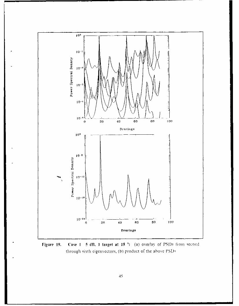
Case I isvi~h all sources at a signal strength of -S dB. Figure 1)shows results from
the second through si'\th eienvectors of a single source at I So. Note that some of thc
elcnvectors have individual peaks as high as the true sigial peak. but only at the true
bearing do all have a common peak. Figure 20 illustrates the other end olthe spectruml.
at S1 . Once ag-in the second throug1h sixth Cicenvectors arc overlax ed to sho\ that the
correct bearing is consistently displayed, but in this case one eioenvector has an irdi-
vidual peak higher than the true signal peak. The product of these PSDs provides suf-
ficient resolution. lieure 21 has two closely spaced sources at 360 and 3S . Resolution
is achieved but the P'SD product of the second through sixth Cigenvectors shows a spu-
rious peak near 75' . Figure 22 is from three sources at 0'. 36° and SS.2 ° . The individual
eigenvector PSDs clearly show the excellent performance at broadside.
Case 2 lowrcs the signal stleneth of all sources to 0 dB. Figure 23 shows results
from zhe second throui: sixthi cienvectors of a single source at IS'. MXanx more peaks
43

I SENSORS
BANDPASS
F FILTERS
CORRE L ATORS
EIGENDECOMPOSITION
SPECFrRALESTIMATOR
BEARINGS
Figure 18. A physical implementation
are visible in the PSI) product. making the (Icciq1o of how many targcts more diflicult.
Figure 24 shows that at the the other end of the spectrum (at SI) the situation is
44
IO-n -1I0 o
10-1
V)
0.C-,
.0
10-4
I 0 - - - - ' ----- -
0 20 40 60 80 1O0
pe a rills
Ion - - ,
106
i0-12
CL.'4C
0 20 40 60 80 10
Bearings
Figure 19. Case 1 5 dB, I target at IS o: (a) overlav of PSl)s tlom second
through sixth cigcn'ectors, (b) product of the above PSI)C
45

100
10-1
C
4)10-.
C,
10-4
0 20 40 60 80 100
len rinTs
10I
10-2
, 10-in
10-4
to-e
I)
o 10-B
I0-9
0 20 40 60 so 00
Bearings
Figure 20. Case 1 5 dB, I target at 81 0: (a) overlay of PSI)s from second
through sixth cigcnvectors, (b) product of the above PSl )s
46

10-1
CL
C' 10-:l
Io I10-7
1 0
l o-9
0 0 4 0Co ID
Be riig
Fim 1. (ae 11.2trg t t 6'ito3 ' a c i o-P I s oliti
tlti- 1 cc t ic~ co-,(,)po u to h b~ S~
C l047

1 0 -
L
fL "N-
I -2
0) 20 -0 110 - oo[0
Fp ~g
Fiur 2. Cle1 M.3 agesat0 ,36 id 8. a)m ily f P D
fl msCn hO Ii ltlCj'f tr,( )po u to h !- cP D
C4

slightly worse (due to a !ower sampling rate). The overlays of the second through si'sth
ei2envectors show that the correct bearing is consistently displayed, but in this case
enough spurious peaks reinforce one another, resulting in the PSD product that has not
zeroed out the bad peaks. Figure 25 illustrates that the proper choice of eigenvectors
will resolve this problem. Here the PSDs of the first through fifth eigenvectors are used.
giving a product that is easier to determine correctly. Figure 26 shows the 0 dB case for
two close spaced sources at 360 and 38°. Resolution is achieved but the PSD product
of the first through fifth eigenvectors shows several spurious peaks, including the same
one as in Case 1 near 75° . Figure 27 is the three source example at 0 dB. The individual
eieenvector PSDs are repeating at the proper bearings but the performance at broadside
is resulting in the product at the other bearings actually bein g driven down.
A signal strength of-5 dB is used for Case 3. Figure 2S shows results from thc irt
ll ejIenvectors of a single source at 1 S'. l.sing more cood eeienvectors increase, the
likelihood that all spurious peaks will be diminished. t igure 29 illustrates results at the
etier end of the spectrulrk (at Wl°). Resolution is looked at in Figure 30. At -5 dB the
algorithm cannot separate the two close -paced sources at 36' and 3S . .A number of
spurious pe,.ks are higher than the bump at 36 making it impossible to accuratel% dc-
terine the num~ber of sources as well as both locations. Resolution is tricd a::in in
Figure 31 with 2 sources at lo, and 4W . U sine five cicenvector PSI) products p':duces
good results. tigure 32 ,hows 3 sources at -5 dl1. Good performance is seen both in
the overllas and in the PSD product.
Case 4 sttrts with I{,} sen ,sors and a 25 by 25 covariance ma trix shown\ in
t-gjure 13. \s the (u),Icr ohsensors is decreaed and the number of eicenvecter, :sed
is held constant, m orC spurious peaks start tu occur (Fligure 34 and iure .
Ficure 36 shows thc ,pctral improvement as more eigenvectors are used As the
number of sensors is dcreasCd to -40 (Figure 37) and seven egeePvectors are used. the
results are still acceptale, t.sing only 3' sensors w e can no longer see rcsolve btveen
the two closely spaced sourLcS. With a sufl'Icient number ofcigenvectors no spurious
peaks are present but the true number of targets is nondeterminable (Figure 3S and
I ]Lure 314

100 ___ _____ _
10-1
W)
10-2
0
10-1
I0-5 -- __________
0 20 40 60 80 100
Bearings
lO-I
10-2
O0-3
10-4Io-A
o jo - 7CL)
i0- -
0 20 40 60 00 100
Bearings
Figure 23. Case 2 0 dB, I target at 18 0: (a) overlay of PSDs from second
through sixth eigenvectors, (b) product of the above PSDs
50

I0-4
20 40 60 o Oo o
llenrinlgqI )
01
10-1
10-4
C to-,-
,n i(o n
0 20 40 60 80 100
Benring
Figure 24. Case 2 0 dIB, I target at 81 : (a) overlay of PISDs from first throuh
fifth e Igc~co (b) product of the second through sixth eigcenvector
n-S-.)s
~5
V

10o 1
10-2
I J 0-3
10 - 4
J.., 10-5
i0-8
o 10-7
10-8
I 0 -9
10-jo0 20 40 60 80 100
Bearings
Figure 25. Case 2 0 dB I target at 81 0: product of the first thiough fifth
cigcnvcctor l'SI)s
52

too
10-
0(L
Sto-i
10-
a 0-
0-
0 20 40 60 0 t
flen rings
clcito SD

10-4.,o2....oo 1 00
100
CL
10-20 20 40 60 60 100
Bearingslo
10-8
C10-12_
Figure 27. Case 2 0 dB, 3 targets at 0 *, 36 ° and 88.2 0: (a) overlay of PSDs
from second through sixth eigcnvectors, (b) product of the above PISDs
54
lil 1llll lll I' f III II II II

to(10-
10-2
L)
I0-4
U
I o-5 t,{) 20 40 60 80 100
100
10-1
10-2
l o-OI-4)I0
to0 20 40 60 s0 too
'0-I
o I0-2
)-
I tO-'f _
., tio-s
Bearings
Figure 28. Case 3 -5 MB I tat-get at 18 °: (a) overlay of PSI~s From first through
,sixthl eigte , ectors, (b) product of' the first 10 eigerivector PSl~s
U5

1O0 ,
10-
:t 10- 3
0
10-
1I0-
0 -0
0 20 40 60 80 1 OO
Bearings
S1-2
SI0-O'U,
0
4
0.
-.
oo2 40 0 8 Io7
ie Brings
Figure 29. Case 3 -5 dB, 1 target at 81 ': (a) overlay of PSI)s From first throughsixth cigcnvectors, (b) product of the first 10 eigenmcctor I'S)s
56

10-1
o10-
l0-5
0 20 40 60 80 100
Benring~q
01)l)
o
10.- 1 -
10-2
10-3
10-4
I 0-n
10- .
0 20 40 60 80 t0o
Bearings
Figure 30. Case 3 -5 dB, 2 targets it 36 o and 38 o:(a) overlay of" PSDs from first
through sixth igenivectors, (b) product of the above IPSDs
57

1,0-
Ven i0_.
100 - - - --
1 o-2"
I)
0-en
1()-
0O-8
10-9
[ -5 / _ _ , _ ,__ _ ,__ _ _
0 20 40 60 00 100
Bearings
o
10-I
1(0-2
SI0-
o- i0-
55)
0-
I.,,a,
o I0(-7
0-
IO-n
0 20 40 60 80 O0
lienrlngn
Figure 31. Case 3 -5 dB, 2 targets at 360o ard 400°: (a) overlay of PSI)s from first
through sixth eigenvectors, (b) product or the first 5 eigcn~ ector lPSl)s

100
[0-I
V
V
10-4
in-s I__
0 20 40 60 00 10
flearlngq100
10-2
.t I0-3
S10-4
S10-5
1o-8c 10-7(L
C.
1 10-8
o10-9LL
i0 _____L
0 20 40 60 80 100
Bearings
Figure 32. Case 3 -5 dB, 3 targets at 0 0, 36 0 and 88.2 0: (a) overlay of PSDs
from first through sixth eigenvcctors, (b) product of the first 10 PSDs
59

100
t0-'
t!
to-
4)-2
06

10-1
10-3
I0-4oI
10-5
0 20 40 60 80 100
Bearingsoo
10-1
I0 2
I 0-3
10-4
10-5
'f lo-5
0 20 40 60 o0 100
Bearings
Figure 34. Case 4 5 dB, 3 targets at 18°',36°' and 41.4: 75 sensors, (a) PSDs
Of sckcolld tillro1u9h sixth eigcnvectors, (b) produ(ct of tihe abovc PSI)s
1001

10-2-
10-3
f0
GO-
m 10-4L
10-5
0 20 40 60 rio 100
Bearingis
10-'
10-410-0
0 10-7
lo-()
10-9
20 IU 60 DJo IOU
bel iiI I f'igsl
Figure 35. C'ase 4 5 dB, 3 targets at 18 ', 36 oanld 41.4 °:50 sensors, (a) PSDs
of' second Cilro,.gh sixth eigerivectors, (b) product oC the above PSDs
62
i i I I I I ~~I-II!I. lG

100
10-1
10-2
10-3
~'10-4)
10 . 6
10-,
10-8
10-9
10-10 -- _____
0 20 40 60 80 100
Bearings
ig ite 36. (ase 4 5 1i. 3 laigets at I ', 36 iand 41.4 "" Pioduc t of the liit
through eighth cigenvector lI)s
63

100-
t:/
S10-2
v
00-
to-',
0 20 40 Go 80 Ion
flenrlngq
10-0
0-1
0.C,,
I0 20 4 6 n o
Bearings
Figure 37. Case 4 5 dIB, 3 targets at 18 O, 36 0and 41.4 40 sensors, 20 by 20
matrix, (a)PSIs of first through seventh eigenvector s, (b) product of
the above PSDs
64
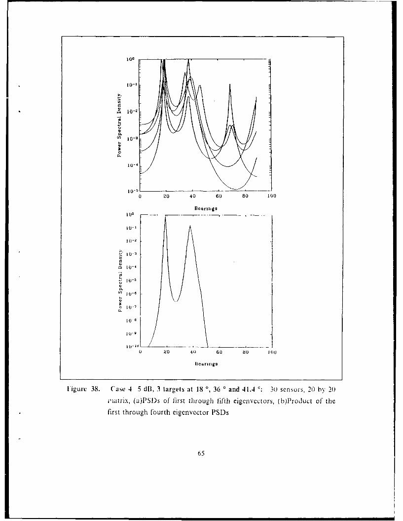
100
10-2
10-3
10-4
10-50 20 40 60 60 IOU
Bearings100
10-1
10-2
10-4
0-5
c 10-7
10-
A 0u
5-65
U -
C O | t
_ , . . .
565

ion
10-24' -20 4 6 0 o
10-2
0 20 40 60 80 t00
Blearings
1066

V. CONCLUSIONS AND RECOMMENDATIONS
Ihle results plotted in Chapter IV indicate that the cicenvectors found using the
Laniczos algorithmi are sufficiently accurate to determine thle spectrum. Although no
direct comparisons with other cigendecomposition methods are performed, thle theory
indicates that many fewer operations are required. We handle the other diff-iculty of
conventional subspace methods by using only a few of the eigenvectors associated with
the mlinimiumy eicenvalues of the autocorrelation matrix. No estimation of the noise
subspace dimension is required or performed.
This theory may be applied to any system. requiring rapid decomposition of the
correlation matrix. Lxanilles include phased array rada r and psieacoustic arrays
lRef's. 30. 31]. Reference 32 details an experimental systemi usinge the NIL's IC algorithml
f'or mli11ple source dirction finldineL.
The following, areas are recommended for I'Ltui-e study.
*I cof the reducts ofru pI pcr ppa rent l% resulted in Lood detc:tion at lokvSN R. MOi ore researh in- this areaL to determline a phyisical Interpretation of' this
* lS,'IL comparison of- thle results in1 tcrnms of computational speed and aLCo-raIcV with otlocr ejeende ccomposition methods should be performed to find the true
C S~ It s.
* 11he Lanlczos aieorfihm develope)d uses no reorthogonalliation nor w Ill it find re-pcano e~cena jes.Other Forms of the Lanc/os ale orithim are ava illa We. ( oam-
pan-iOr, sonsbtween theseL dil1'erent methods to determine1 IccLura cv anj-d speed Ia\.lead to mnore op tim ull results.
*A in tIer edtil odel should he developed that will simulate an arri wit i h-inkof bandlpaslis er to 1hctter forecast results of' a phy\sical ilnctt nas sen
A w\ et, od whlicht 11i lnent s the lgith in parallel fliion mayi be trid k2 inone loll neli r arm -scerl overla ppin1,- subarraxs may tie use d to t, mul A neon Nb
create several aut ocor-rela tioln matrices. 'Ihle al son thinl mayc be applied to thesematrices InI parallel. It is predic:ted that thle greater numbecr of' availableeILeenIVeC tors Will1inore prprydscibe1 the noiseC subspace anid therefore inore
accratly stiatethe pCtr
(6
LIST OF REFERENCES
I.Kav. Steven M., Mlodern Spectral Estmation, Prentice-liall, Englewood Cliff-s. 19S'7
2. Schmnidt. Ralph Otto, "A signal subspace approach to multiple emitter location and
spectral estimiation," Ph.D. Thesis, Stanford Universitv, Stanford, California, Nov.
1981
3. Kay. Steven M.. and Stanley Lawrence 'Marple, Jr., "Spectrumn analysis--a modern
perspective." Proceedings of the IELE. Vol. 69, no. 11, Nov. 19S81, pp. 1"SO- 1419
4. Orphanidis. Sophocies J.. Optimum Signtal 1rocessitig, An Intrw.'ucti;, 2d ccl.
Nlacnmiilan. New York. 9S5
5. \la-1p c. S. Luwrcnce. Jr.. JDig'iu! .spe'ca'C . lnzsP ih.4pi~i;,Iren::ce-l 1a1.
linelwoodCiV5.' 19S7
6. Kay. Steven. and Cedric 1)emeure. "The hiehi-resol ution specltruml estima'tor-a
subjectiv e entity." 7rNcazso h 1666 Vl 2 no). 12. -C. I W- 1
7. Lirris. Ircdric J ., 'On the use of windowsk- for har11moniJc Z1n11%1 %Vwjll theC C11"crete
fo uier ransorm" 1~m'ccba~' firiic 1161616. Vol. 06. no. 1, J an. 1) S. pp1. I-S
S. Nuztail. A\lbert 11.. "Somle windows w ith very Lood siJelobe hcu.jr"111616 i*)t;1o.
on7 A.S.SP, Vol. ASSP-29. 1no.1, 1 C. 19M1. pp. S-4-91
9. V'an V'een. Barry ID., and R ich~ard A. Roherts. "Partialvy adaptive hcaml'ormcr de-
sinz via output power rniinizatiOn." IEEEL 1tans. (1 . S. V\'. .ASSP-3 5. nIO. 11.
No0v. 1K p)nS 1524-153 2
I (. Van Veen. B~arry D).. and Kevin M. Buckley.,Iemfrlc a %ersaJti~c aprca,,h
to Spati-l filterinc." 11-1616 AlSS1, V\a"abr V'ol. 5, io. 2. A\pr. 11)',S. pp. 4-24

11. Dudgeon, Dan E.. and Russell M. M ersereau, .1lultidiniensional Digital Signal
Processing. Prentice-H1all, Englewood Cliff's, 19S4
12. Schmidt. Ralph 0., "New mathematical tools in direction finding and spectral
analysis," Proceedings of SPIE, Real Time Signal Processing J IT Vol. 4131. Aug.
23-25, 1983, San Diego, CA, pp. 7-19
13. Schmidt, Ralph 0., "Multiple emlitter location and signal parameter estimation,"
IEEE Trans. on Awi. andi Prop., Vol. AP-34, no. 3, Mar. 1986, pp. 276-280
14. Paulra', A., R. Roy, and T. Kailath. "Estimation of Signal Parameters via Rota-
tionail Invariance Teelmiq ues--E SPR IT," Proceedings, (,f' he l1th .-Isiloinar Cco!'. on
C/crs.. St'st.. ana Comp., Pacific Grove. I 9S6. pp. S3-S9
15_. Golub. Gene 1L.. and Charles F. Van Loan. Hatrix Coinzpuiauiuns. Johns Hopkins
Press. Baltimlore. I 0S3
16. Kumairesan. Ranldas. and Arnah) K. SIaw. "SUperrecsolution b% ,truiCtul1_d mat~rix
* alroxinlation. IE-E TFLUZs. on .-1SSP> Vol. ASSP-36. no' 1, Jan. 1988, pp. 3-4- 4
1. Nikitakos. Nikitas V., "A comlpatrison of two frecquenc\ domain adaptive
bcan!'or~2~al-orithis for sonar signal processin, ' NI aster'sih i~ Naval1 Pest-
Llraduate School. NI ontcr%2v. Californi, I 988
I. iIalpeniv. Owen S.. anld Donald G. Childers. "Comiposite \vavef'ront decenm.oSinon)1
viat Imultidimen~sional di1i aI 1terin e of' arrav data.", IEE l Pios. ,I/ CA is. 1 ld
S.VA!.. Vol. (iAS-22. Jun., 11)-5. pp. 276-_286(
19. Cadt.ow. .Jaines A.. "A liigh resolution Direction-ofArrival alcorithin for narrow-
band coherent and in1O1cherent souirces," IL.' Tra;,s. on .ASI', V'ol. 36. no. 7, Jul.
1988. pp. 965-979
20. Johnson, Don lI., and Stuart R. DeGraaf. "Improving the resolution bearing InI
pass-iveC sona1r aIrrayVs b% CqicenValLIe aayiLilE irons. ofi .lISSP. Vol. ASSP-310.
no. -4. .'\ug. 19>2. S 63- )4 7
21. Lanczos, Cornelius, Applied lnalhsis, Prentice-I lall, Englewood Cliffs. 195%
22. Lanczos. Cornelius, "An iteration method for the solution of the eigenvalue prob-
lem of linear differential and integral operators," Journal of Research Mfthe .Vational
Bureau of Standards, Vol. 45, no. 4, Oct. 1950, pp. 255-282
23. Cullum, Jane K., and Willoughby, R.A., Lanczos A1gorithms for Large Sv'nI,,etrc
Eigenvalue Computations, Vol. 1, Birkhauser, Boston. 1M85
24. Tufts, D. and Melissinos, C.D., "Simple, effective computation of principal
eieenvectors and their eigenvalues and application to high-resolution estimation of
frequencies." lEEF Trans. on ,ISSP. v. ASSP-34, no. 5. Oct. 1986, pp. 1046-,053
25. l'tigc. C. C.. "Computational variants of the Lanc/os method for theeieproblem." J. Inst. .lah. .tpp1 ., 10. 1972. pp 3'3-381
2. Paige. C. C.. "'Ihe computation of eigenvalucs and eicenvectors of very large sparse
n a:rices.' Ph.D. Thesis. Lnivcrsitv of Londoni. London. Lngland. 1971
2-. Pariett. B. N., Di .t' nmetric Kigcn'alut',b em, P;-rentice-lail. In!C\wood Cliffs.
28. PaiLc. C. C.. "ccuracy and effectiveness of the Lanc/os aicorithm0 lor the s'In-
n~c tri. c1g prc, Vnic. ,',' lfar .1!izc/'hra and its .lp,''' w'ios 34, .c'ican A inck ,cr
21). Cuill.'", Jane K.. and W.illoughby. R A., LaCII:,,s .1!,o.',ii-,z's./,r 1. w ce .';,,,ctric
Ll t'nl l,' a ~lt nutaiols, l'ol. 2, Birkhauser, Boston, 1 ) .S5
3'. NiLkcl. .. ngular superresolution with phased array radar: a review of a!,ico-
rithn> and operational constraints. IEE Proc.. Vol. 13-. PT. F. No. 1. 1 cb. I)S".pp. 53-5"
31. .ialapaw Rss . crt L ... 'A:\ .\S: 13iL -\S\ help for small ships, .5..'; .,.
N,, ,,' \ )!. 115 1 l 31. Ii S ). pp. 107-1 lo
7'i

32. Schmidt, Ralph 0., and Raymond E. Franks, "Multiple source DE signal process-ing: an experimental system," IEEE Trans. oa Ant. and Prop., Vol. A\- 34, no..
Mar. 1986, pp. 281-290
SI
"'1

INITIAL DISTRIBUTION LIST
\o. Copies
1.Def'ense Technical Information Center2Cameron StationAlexandria, VA 22304-6145
2. Librar-y, Code 0142 2Naval Posturaduate School.Monterex', CA 93i943-5002
3. Chairman. Code 621Department of E lectrical and Computer E~ngineeringNaval Postsraduate SchoolNlontere\. CA: 93943-50 ()
4. Professor NIurali T- mn-ala. Code 62TuDepnartment of Flctilcal and Computer EngineermolLNaval Posturatduate schoolNlontcrcv. CA 93Q.41-5000
5 . P, ofessor C. WV. Therrien, Code 62Ti1Departm11ent of' Eilectrical and Comlputer Filgninerin e,.Na\ 1i Po~trraduatle schoolMonterey. CA 93943-500w
6. ProfeNsor Ralph I lippenwtiel. Code (02111iDepatmen~~lt of I ',1 ilc rcMIad Computer E ngineering-N av~al lPosr orudna te school
Navl )canS% stes enterSa11 DiCco. CA. ~ I -3
S. D)r. Rahi) MIada n(h tice of Naval ReseCarchiCode 14
50North Quincy StreetArlin-ton, VA 222l7~-,5(,()
9. Daniel [F. Gear 4-10-1 Nervine StreetMIonterev, CA 919-40
10. Yonc Jon KimSNIC IT
NtAva Posterajulate SchoolN Ion terev. (' q\~3)4~)( )()
Recommended