AN INVESTIGATION OF SATELLITES TO THE RESONANCE LINES
IN SOME HYDROGEN-LIKE IONS
by
Nelson Wayne Jalufka
B.S., Lamar University, 1962
M.A., College of William and Mary, 1967
(NASA-TM-X-68338) AN INVESTIGATION OFSATELLITES TO THE RESONANCE LINES IN SOMEHYDROGEN-LIKE IONS Ph.D. Thesis - Colo.Univ.. N.W. Jalufka (NASA) 1972 181 p
_- CSCL 20H G3/24
N72-256U49
Unclas30539
A thesis submitted to the Faculty of the Graduate
School of the University of Colorado in partial
fulfillment of the requirements for the degree of
Doctor of Philosophy
Department of Physics and Astrophysics
1972
https://ntrs.nasa.gov/search.jsp?R=19720017999 2020-04-28T00:56:27+00:00Z
This Thesis for the Doctor of Philosophy Degree by
Nelson Wayne Jalufka
has been approved for the
Department of
Physics and Astrophysics
by
John Cooper
Date
iiiPRECEIING PAGE BLANK NOT FILM ED
ABSTRACT
Jalufka, Nelson Wayna (Ph.D., Physics)
An Investigation of Satellites to the Resonance Lines in Some
Hydrogen-Like Ions
Thesis directed by Professor John Cooper
This research has been an experimental and theoretical investi-
gation of the origin of satellites to the resonance lines of the
hydrogen-like ions of boron, carbon, and nitrogen.
A theta pinch was employed in conjunction with a grazing inci-
dence spectrograph to measure the wavelengths of the satellites.
The spectroscopic data also provided an estimate of the satellite to
resonance line intensity ratio.
Wavelenghts of spectral lines due to transition from doubly
excited states were calculated by a Hartree-Fock computer program.
Wave-functions were also calculated by this program and were used to
obtain the oscillator strengths of the transitions.
Calculations of the upper limit of the satellite to resonance
line intensity ratio showed that the observed intensity of the
satellites was much greater than could be explained by present theo-
ries, and further experimental work confirmed that the lines investi-
gated were not satellites but were due to highly ionized argon which
was present as an impurity in the filling gas of this and many
previous experiments.
This abstract is approved as to form and content. I recommend itspublication.
SignedJohn Cooper
iv
ACKNOWLEDGMENTS
I would like to express my appreciation to my advisor, Professor
John Cooper, for the support, encouragement and the instruction that
he has given me.
Thanks are due to Dr. Louis Shamey for his instruction and
help with the computer programs.
I would also like to thank Mr. John Fryer for his very able
assistance with the operation of the theta-pinch facility and Mr.
M. D. Williams for his help in locating and correcting the problems
associated with the operation of a large capacitor bank.
Special thanks are due to Bob Alvis and his staff at JILA for
their courteousness and help.
Thanks are also due the Langley Research Center of NASA for
the support given me during the course of this investigation.
This research was supported by the Physics and Astronomy Program
at NASA Headquarters, Washington, D. C. and I am grateful to Dr.
Goetz Oertel for this support.
Finally I would like to thank my wife, Jean, for her encourage-
ment and understanding.
V
TABLE OF CONTENTS
Chapter Page
I. INTRODUCTION . . . . . . . . . . . . . . . . . . . . . . 1
History . . . . . . . . . . . . . . . . . . . . . . . 1Application to Astrophysics. . . . . . . . . . . . . . 3
II. THEORY AND CALCULATIONS .. . . . . . . . . . . . . . . 7
Multi-Electron Atoms and the Central FieldApproximations. . . . . . . . . . . . . . . . . . 7
The Variational Method ......... .. . 17The Self Consistent Field and Hartree's Equations. . . 21Hartree-Fock Equations .............. . 25Calculations .................. .... 38
III. ATOMIC PROCESSES AND PLASMA MODELS . . . . . . . . . 46
Ionization Processes and Rate Equations . . . . . . . 46Bound-Bound Transitions and Rate Equations . . . . . . 51Doubly Excited States and Dielectronic Recombination . 53Equilibrium Relationships and Detail Balance . . . . . 57Applications to Laboratory Plasmas . . . . . . . . . . 63
IV. EXPERIMENTAL METHOD . . . . . . .. . .81
Theta-Pinch Device . . . . . . . . . . . . . . . . . . 81Grazing Incidence Spectrograph . . . . . . . . . . . . 99Data Analysis . . . . . . . . . . . . . . . 115
V. RESULTS AND CONCLUSIONS . .. . . . . . . . . . . . . .119
Results With Boron and Carbon . .. . . . . . . . . .119Results With Nitrogen . . . . . . ...134Conclusions and Limits of Laboratory Experiments · · *136Suggestions for Further Work .......... . 139
BIBLIOGRAPHY . . . . . . . . . . . . . .141
FIGURES. . . . . . . . . . . . . . . . . . . . . . . . . . . . .147
vi
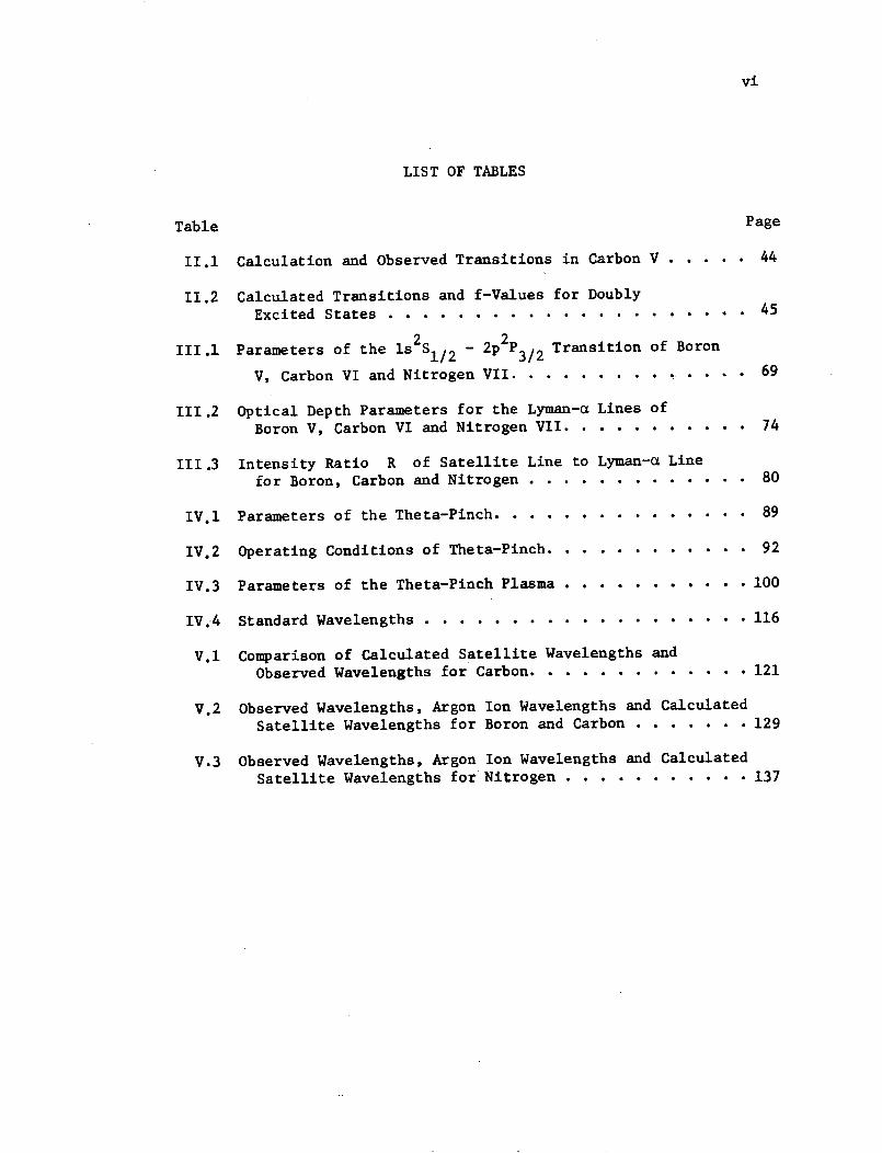
LIST OF TABLES
Table Page
II.1 Calculation and Observed Transitions in Carbon V ..... 44
II.2 Calculated Transitions and f-Values for DoublyExcited States ................... .. 45
III.1 Parameters of the lsS1/2 - 2pP3/2 Transition of Boron1/2 3/2p 2 Transition of Boron
V, Carbon VI and Nitrogen VII . . . . . . . . 69
III.2 Optical Depth Parameters for the Lyman-a Lines ofBoron V, Carbon VI and Nitrogen VII. . . . . . . . ... 74
III.3 Intensity Ratio R of Satellite Line to Lyman-a Linefor Boron, Carbon and Nitrogen . . . . . . . . . . ... 80
IV.1 Parameters of the Theta-Pinch. . . . . . . . . . . .... 89
IV.2 Operating Conditions of Theta-Pinch. . . . . . . . . . . . 92
IV.3 Parameters of the Theta-Pinch Plasma . . . . . . . . . . . 100
IV.4 Standard Wavelengths ................... 116
V.1 Comparison of Calculated Satellite Wavelengths andObserved Wavelengths for Carbon. . . . . . . . . . . 121
V.2 Observed Wavelengths, Argon Ion Wavelengths and CalculatedSatellite Wavelengths for Boron and Carbon . . . . . 129
V.3 Observed Wavelengths, Argon Ion Wavelengths and CalculatedSatellite Wavelengths for Nitrogen . . . . . . . . 137
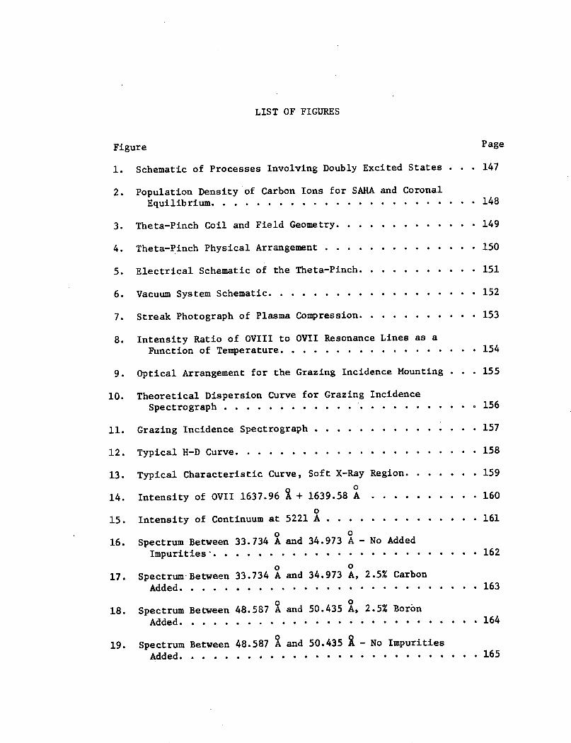
LIST OF FIGURES
Figure
1. Schematic of Processes Involving Doubly Excited States
2. Population Density of Carbon Ions for SAHA and CoronalEquilibrium . . . . . . . . . . . . . . . . . . . . . . .
3. Theta-Pinch Coil and Field Geometry . . . . . . . . . . . .
4. Theta-Pinch Physical Arrangement . . . . . . . . . . . . . .
5. Electrical Schematic of the Theta-Pinch . . . . . . . . . .
6. Vacuum System Schematic . . . . . . . . . . . . . . . . . .
7. Streak Photograph of Plasma Compression . . . . . . . . . .
8. Intensity Ratio of OVIII to OVII Resonance Lines as aFunction of Temperature . . . . . . . . . . . . . . . . .
9. Optical Arrangement for the Grazing Incidence Mounting
10. Theoretical Dispersion Curve for Grazing IncidenceSpectrograph . . . . . . . . . . . .. . . . . . . . . . .
11. Grazing Incidence Spectrograph . . . . . . . . . . . . . . .
12. Typical H-D Curve.
13. Typical Characteristic Curve, Soft X-Ray Region . . . . . .
14. Intensity of OVII 1637.96 A + 1639.58 A . . . . . . . . . .
o15. Intensity of Continuum at 5221 A . . . . . . . . . . . . . .
o 016. Spectrum Between 33.734 A and 34.973 A - No Added
Impurities . . . . . . . . . . . . . . . . . . . . . . . .
O o17. Spectrum-Between 33.734 A and 34.973 A, 2.5% Carbon
Added . . . . . . . . . . . . . . . . . . . . . . . . . .
18. Spectrum Between 48.587 A and 50.435 A, 2.5% BoronAdded . . . . . . . . . . . . . . . . . . . . . . . . . .
19. Spectrum Between 48.587 A and 50.435 i - No ImpuritiesAdded . . . . . . . . . . . . . . . . . . . . . . . . . .
Page
147
148
149
150
151
152
153
154
155
156
157
158
159
160
161
162
163
164
165
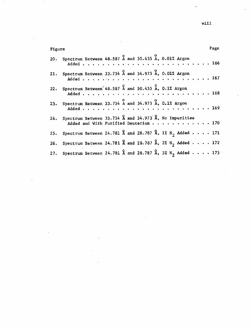
Figure
0 020. Spectrum Between 48.587 A and 50.435 A,
Added . . . . . . . . . . . . . . . .
21. Spectrum Between 33.734 A and 34.973 A,Added . . . . .. . . . . . . . . . .
22. Spectrum Between 48.587 A and 50.435 A,Added . . . . . . . . . . . . . . .
O 023. Spectrum Between 33.734 A and 34.973 A,
Added . . . . . . . . . . . . . . . .
24. Spectrum Between 33.734 i and 34.973 i,Added and With Purified Deuterium . .
25. Spectrum Between 24.781 A and 28.787 A,
26. Spectrum Between 24.781 i and 28.787 A,
27. Spectrum Between 24.781 and 28.787 A,
0.01% Argon0.01% . . .Argon
0.01% Argon. . . .. . .
0.1% Argon. . . . . . .
0.1% Argon. . . . . . .
No Impurities1. . . . . .
1% N2 Added
2% N2 Added .
3% N2Added .
viii
Page
. . . 166
. . . 167
. . . 168
. . . 169
. . .170
. . . 171
. . . 172
. . . 173
CHAPTER I
INTRODUCTION
A. History
Long-wavelength satellites to the resonance line of a hydrogen-
like ion were first observed in the laboratory by Compton and Boyce
(1928). They reported two weak satellites to the resonance line of
singly ionized helium and suggested that these lines were due to the
excitation of both electrons of neutral helium into the n = 2
level and the radiation accompanying the return of one electron to
the ground state. This explanation was later confirmed by theoreti-
cal calculations (Kiang, Ma, and Wu, 1936).
Edlen and Tyrin (1939) published a vacuum spark spectrum of
carbon covering the region from 60 2 to 15 2. It was expected that
the spectrum in this region would be very simple, consisting of the
normal helium-like and hydrogen-like series. However, a considerable
number of additional lines appeared in distinct groups to the long-
wavelength side of the helium-like and hydrogen-like resonance lines.
The proximity of these lines to the resonance lines indicated that
they were due to transitions of essentially the same type as the
resonance transition but at a slightly lower energy. These lines
were explained by transitions of the type
ls2 nZ - ls 2p nt (1.1)
2
for the helium-like satellites and
is nZ - 2p nX (1.2)
for the hydrogen-like case. This explanation appeared reasonable as
the presence of the additional outer electron would reduce the
potential field in which the transition takes place and, consequently,
cause a shift to longer wavelength. The prominent satellites were
attributed to n = 2, as those with greater n would rapidly move
nearer to, and merge with, the resonance line. As a consequence of
this explanation, the existence of discrete energy levels, lying
well above the ionization limit of the ion in which the transition
takes place, had to be assumed.
More recently, the observation of such satellites has been
reported from a number of laboratory plasmas, including sparks
(Flemberg, 1942; Feldman and Cohen, 1969; Goldsmith, 1969; Lie and
Elton, 1971), high-temperature pinches (Sawyer, 1962; Roth and Elton,
1968; Peacock, Speer, and Hobby, 1969; Gabriel and Paget, 1972;),
and laser-produced plasmas (Gabriel, 1971). The observation of
similar satellites in recent solar spectra (Fritz, et al., 1967;
Rugge and Walker, 1968; Jones, Freeman, and Wilson, 1968; Walker and
Rugge, 1970) has led to a renewed interest in the origin of these
lines.
3
B. Applications to Astrophysics
In order to establish the importance of doubly excited states
to problems of astrophysical interest, it is first necessary to
investigate the physical processes by which these states may be
populated and depopulated. This is necessary since most astrophy-
sical plasmas cannot be described in the limited framework of thermo-
dynamic equilibrium and a knowledge of the rate coefficients of the
different competing processes is important in determining such
properties as ionization balance as well as the distribution of
electrons among the various energy levels of the atom or ion.
Doubly excited states may be populated, as well as depopulated,
by electron collisions. Photoexcitation may also populate these
states. The inverse processes is spontaneous and stimulated (if a
radiation field is present) emission. Spontaneous emission is the
process responsible for the emission of the satellite lines. A
more interesting process, for the formation of the doubly excited
state and the one that was the basis for this research, is inverse
autoionization. In this process an electron combines in a radiation-
less transition with an ion of charge Z to form an ion of charge
Z - 1 in a doubly excited state. The doubly excited state then
decays by spontaneous emission and the two step process is called
dielectronic recombination These two processes are not applicable
to all doubly excited states, as certain selection rules must be
obeyed. These selection rules which consist of conservation of
energy, total angular momentum, and parity will be discussed in
Chapter II.
4
Transitions between doubly excited states, which may undergo
autoionization and normal (singly excited) states, have several
astrophysical applications. The natural width of such lines are
often much greater than widths due to random Doppler broadening
or collisional broadening, since the lifetime to autoionization is
often small. This large width makes these lines very efficient
absorbers of radiation, as they will only become saturated at
relatively large values of the equivalent width. There is a very
large probability that each absorption of a photon in the line will
be followed by ionization, so that the mechanism of line formation
is pure absorption. This greatly simplifies the analysis.
The astrophysical importance of dielectronic recombination has
been pointed out by Burgess (1965a). This process is, perhaps, the
most important role played by doubly excited states in astrophysical
situations. The problem which led Burgess to examine the process
in sufficient detail to realize its importance was the discrepancy
between the temperature of the Solar Corona as deduced from the
observed widths of the "forbidden" emission lines of FeX, FeXIV, and
CaXV and as deduced from ionization balance calculations. The
widths of the emission lines were interpreted as Doppler widths and
indicated a temperature of about 2 x 10 K (Evans, 1963). The
ionization balance calculations were carried out by balancing the
rates of ionization due to electron collisions and the rates of
recombination, which was assumed to be radiative. These calculations
indicated a temperature of 106 OK. The factor of two discrepancy
5
does not, at first, appear to be serious. However, in order to
bring the calculated temperature into agreement with the Doppler
temperature the recombination rate had to be increased by a factor
of 30. The same results could have been achieved by decreasing the
ionization rate by the same factor. Careful examination of this
process however, revealed that the ionization cross section used
was essentially correct since the theoretical values were verified
by experimental measurements. Burgess performed detailed calcula-
tion of the dielectronic recombination rates for many elements in
various stages of ionization. These calculations showed that if the
temperature was high enough so that a substantial fraction of free
electrons could make radiationless transition to doubly excited
levels with large principal quantum number, then the total rate
coefficient summed over many levels close to the second and higher
series limits might exceed the corresponding rate coefficient for
radiative recombination by one or more orders of magnitude. These
results were applied to the Solar Corona and were successful in
removing the discrepancy in the temperature.
The processes of autoionization and dielectronic recombination
have also been shown to be of importance in the interstellar medium
(Goldberg, 1966). In particular, a discrepancy exists in the Ca/Na
abundance ratio of the interstellar medium. Analysis of inter-
stellar line intensities leads to a Ca/Na abundance ratio of about
0.03, whereas its value in the sun and other stars is about 0.70
6
which is a factor of 23 larger (Aller, 1963). The observed inten-
sities are for the D lines of NaI and the K lines of CaII. Since
NaII and CaIII are expected to be the most abundant ionization
stages, determination of the abundance ratio requires a knowledge
of the ionization balance. The interstellar ionization theory
developed by Stromgren (1948) depends on an ionizational balance
between photoionization and radiative recombination. The abundance
discrepancy has been attributed to a lack of knowledge of the
stellar ultraviolet radiation field which determines the photo-
ionization rate. However, it now appears possible that the photo-
ionization rates may be in error because they do not take into
account transitions in NaI and CaII from their ground states to
levels which undergo autoionization. It is not clear if the
inclusion of these transitions will clear up the abundance ratio
anomaly. In any case however, the effects of autoionization must
be taken into account if the ionization equilibrium of the inter-
stellar medium is to be properly discussed.
CHAPTER II
THEORY AND CALCULATIONS
A. Multi-Electron Atoms and the Central Field Approximation
An analysis of the radiation emitted by a plasma requires not
only a knowledge of the various atomic processes which occur in
the plasma but also attention to the details of atomic structure.
Calculations of the energy levels of the various atoms or ions in
the plasma must be carried out in the context of a well defined
model of atomic structure. The details of the model which was
employed in this investigation will now be developed (Slater,
1960).
The general Hamiltonian (in atomic units) for a multi-
electron atom may be written (including only the spin-orbit
relativistic term)
H [1 V2 - Z ]+ E 1 +E (ri)Li ' Si ( 2'
1 )
i ij i
alternatively
H = Ho + H1 + H2 (2.2)
with two alternative ways of expressing the components. The general
expression is given first followed by the central field approximation
expression in brackets,
1 _
r__(- i - v(ri) +rij r isi~j
H2 H2 = (r i )Li Sii i
1 1 V(r i)£(ri2 2 2 r ar
2m c i i
where V(ri) is the approximate central field in which the elec-
tron moves (Shore and Menzel, 1968).
The term H is just a sum of terms which are the Hamil-
tonians of single,spinless electrons moving in a central force
field. Schrodinger's equation for such an electron treated as a
point charge is
H0 [ V2+ Vo(r )] = E0
where
only.
(2.6)
Vo'(r) is the potential field and is a function of Irl
Since the atomic nucleus and the electron possess a charge,
(1 V2 -
2 ri 1 + V(-
i
8
Ho = E
i
and
H1 A-iij
and
(2.3)
(2.4)1i
with
(2.5)
9
the potential function of particular interest in atomic struc-
ture theory is the Coulomb potential (in atomic units)
zV (r ) Z= -r. (2.7)
with z equal to the nuclear charge. Equation (2.6) then
becomes Schrodinger's equation for the one electron atom (hydro-
genic) and has the great advantage of being both separable and exactly
soluble, that is, exact analytic solutions for the eigenfunctions
can be found. The eigenfunctions of H are well known
*(n,k,mz) = R n(r)Yim(e,0) (2.8)
which is just the product of a radial function
Pnk(r)REn(r) = r (2.9)na~ (r ) = r
and a spherical harmonic YQm(0,A). The radial function is
Pn (r)R (r) = (2.10)
with
(n - -- 1);z 1/2 +1 X 2Y+1_--3 ( )Ln+P (X) (2.11)
Pi(r) n2 [(n + )] 1/2 x+lexp ( 2L+1
10
The quantity L +2 (X) is the Laguerre polynomial with
X = 2zr (2.12)n
The function Ph (r) is normalized in the sense that
(r)dr = 1 (2.13)
0
and the spherical harmonics Ykm(8,~) are normalized in the sense
that
/jIYm (e8, ) 2dQ = 1 (2.14)
The total wavefunction ~(nZm2 ) is normalized and also
orthogonal
*(ndue to the ortho')(nmnoral)dV =
nproperties on6f the Laguerre polynomials
due to the orthonormal properties of the Laguerre polynomials
and the spherical harmonics. The eigenfunctions of the one
electron atom are designated by the principal quantum number n,
the orbital angular momentum 2, and the projection of 2 on
the z-axis, mi. Thus the eigenfunctions are mutual eigenfunctions
of the three commuting operators Ho, L , and Lz
with eigen-
values Eo, 2(2 + 1), and m i respectively.
11
When more than one electron is present the potential function
in H°
is no longer the Coulomb potential due to the presence of
the other electrons,however the separable form of equation (2.8)
is still appropriate. The term Hi, which includes the interaction
between the electron of interest and all the other electrons in
the atom,is no longer zero so that Schrodinger's equation,
including H1, is neither separable nor solvable in closed ana-
lytical form. Therefore,approximation methods must be employed
to obtain eigenfunctions of Schrodinger's equation. These
approximation methods are based on the central-field model for
the atom. The central-field model was developed concurrently
with wave mechanics and quantum mechanics. The development
started.with Bohr's first proposal (1922) for the explanation of
the periodic table and was supplemented by the discovery of the
electron spin by Uhlenbeck and Goudsmit (1925, 1926) and by the
exclusion principle of Pauli (1926). The method was completed
with Hartree's proposal (1928) of the method of the self consis-
tent field and with the so-called Hartree-Fock method (V. Fock,
1930a, 1930b, Slater 1930).
Three postulates are required for the central-field model.
The first of these follows from wave mechanics and is merely an
approximation method of solving Schrodinger's equation for the
many body problems of N electrons moving about a nucleus of
charge z units. The other two postulates are extensions of the
wave mechanical principles and are the postulates of the electron
12
spin and of the exclusion principle. The latter two postulates
are required since the electrons are Fermions (spin of 1/2) and
are therefore represented by anti-symmetric wavefunctions which
require that no two electrons occupy the same state.
The simple central-field model in fact,consists of replacing
the instantaneous action of all the electrons of an atom on one
of their number by the much simpler problem in which each electron
is assumed to be acted on by the average charge distribution of
each of the other electrons. This average charge density is
obtained by taking the quantity ~*~ for the corresponding wave-
function, summing over all the electrons in the atom and taking
a spherical average. The potential, arising from this spherically
averaged charge distribution and the nucleus, is itself spheri-
cally symmetric or, in other words, a central field. Eigen-
functions of Ho may then be found since V(r) is now a central
field. These eigenfunctions which represent single electrons
moving in the central field are very nearly those obtained for the
one electron atom [i.e., p = Rnz(r)YQm(6,~)] since the angular
dependence will be the same. The radial part of the wavefunction,
however, may be different. The eigenfunctions of Ho therefore
represent the individual electrons and designates each with a
particular n, Q, and mj. By specifying n and 2 for each
electron, a configuration is denoted in this approximation. The
simplest wavefunction which is an eigenfunction of H is ao
product function of the one electron wavefunctions. This product
13
function will have a well defined parity with the property
('p ). = T (2.16)
where the parity operator P commutes with H . Equation (2.16)
shows that the only eigenvalues of P are + 1 with the eigen-
function -1 called odd parity and + 1 even parity. For the simple
product function the parity is given by
+ =(_ E i?= (-1) i(2.17)
and is determined by the orbital angular momentum of the electron
obtained from the central field approximation. The one electron
wavefunctions must also contain a function of spin since the elec-
tron spin is postulated in the central-field approximation. The
spin function is taken as an eigenfunction of the operators S
and S with eigenvalues 3/4 [ = s(s + 1)] and m ,
respectively. The product of the one electron wavefunction and
the spin function are designated spin-orbitals and are represented
by
u(nRmQSms) -= W(n mt) X (s) (2.18)
+ 1where X (s) are the spin functions corresponding to ma = + 2.
The operators S2 and Sz commute with Ho, L2, L and P since
14
they operate in a different space so that the spin orbitals are
eigenfunctions of these operators.
The coupling of the various orbital and spin angular momenta
may be carried out in the Russel-Saunders or LS coupling scheme.
In this scheme the individual orbital angular momenta of the
electrons is added vectorally to give a total orbital angular
momentum
+L = E li. (2.19)
i
The individual spins add in the same manner to give a resultant
spin
= E (2.20)i
The specification of L and S denotes a term in a given
configuration.
The terms H1 and H2 in the Hamiltonian are treated as
perturbations with the assumption that they make small corrections
to the total energy of the atomic state. This is not always the
case but for many atoms (especially the ligher ones) it is a very
good approximation. The operator H1commutes with L and S
122and with J where
J = L + S (2.21)
15
is the total angular momentum and the operator J2 has the eigen-
values j(j + 1). The operator H1 also commutes with the parity
operator and therefore matrix elements of H1 between functions
of the same J and parity will be non-zero. Thus the interelectron
Coulomb repulsion will mix the single particle product functions
(i.e. spin orbitals) and the concept of a configuration loses its
identity. The existence of these non-zero matrix elements of H1
between levels in different configurations is referred to as con-
figuration mixing. While the effect of the operator H1 can
often be ignored, in many practical cases it can lead to rather
interesting phenomena. The most interesting case and one which
is of interest in this investigation is when one of the configura-
tions contains continuum states. The mixing of bound and con-
tinuum states leads to the phenomena of autoionization as well as
its inverse. These processes involve doubly excited states and
will be discussed in detail along with the other atomic processes
in Chapter III.
The spin angular momentum of the electron may interact with
the orbital angular momentum so that the operator H2
is non-
zero even for hydrogenic atoms. The one electron spin-orbitals
u(nkmQ ms) are not eigenfunctions of H2 since H2 does not
commute with Lz or Sz. The operator H2 does commute with J
and Jz but not with L and S . The eigenfunctions of H2should
2therefore also be eigenfunctions of the operators H, j2 and Jztherefore also be eigenfunctions of the operators Ho, J and iZ
16
Such eigenfunctions may be constructed from the one electron spin
orbitals by using the Clebsh-Fordon coefficients to couple L and
S (Shore and Menzel, 1968)
(2.22)u(nksjmj) = L C(Zsj; mimsmj)u(nkmksms) (2.22)
where C(Zsj; mQmsmj) is the Clebsh-Gordon or vector coupling
coefficient.
Matrix elements of the spin orbit interaction operator H2 are
tabulated by Condon and Shortley (1938) for various configurations.
Since H2
does not commute with L or S they are no longer
"good" quantum numbers. However, the total angular momentum J
is a "good" quantum number as the matrix elements of H2are dia-
gonal in J (i.e,,H2 and J commute). For the levels considered
in this investigation the effects of configuration interaction
and spin-orbit interaction were found to contribute very small
corrections so that the levels are labeled in the LS notation.
It has been pointed out that the one electron eigenfunctions
in the central-field model differ from the hydrogenic functions
only in that the radial dependence is different. These radial
functions must be determined if the eigenfunction is to be a
reasonable approximation to the true eigenfunction. A most useful
procedure which has been employed with a large degree of success
is the variational principle of wave mechanics.
0
17
B. The Variational Method
The variational method assumes that a function W exists
which is variable at will subject only to the condition that it is
always normalized. The average value of the Hamiltonian operation
H for this function is
H avg fW*HW dv (2.23)
where the asterisk denotes the complex conjugate. The function
W is then allowed to vary to W + 6W where both W and 6W are
functions of the same variables and 6W is small relative to W.
An arbitrary change in W will in general destroy its normalization
so that equation (2.23) is not correct for an unnormalized function.
In the general case where W is an unnormalized function the
corresponding normalized function is
(fW~ dv) 1/2 (2.24)
Equation (2-23) should then be more properly written
fw*HW dvH (2. 25)avg W*W dv
The function W is then replaced by W + 6W with the corres-
ponding value of Havg being Havg + 6Havg. If terms of second
and higher order are discarded, and expression for 6H may beavg
18
obtained
HW* + SW*)H(W + 6W)dv6H = Havg f(W* + 6W*)(W + 6W)dv avg
- f6W*HW dv +JW*H6W dv - Havg( W*W dv + w*6w d
+ higher order terms (2.26)
It has been assumed that the unvaried function W was norma-
lized. The variational principle requires that H be stationaryavg
(i.e., 6H = 0) so that H is a minimum for the function W.avg avg
To accomplish this,use is made of the fact that H is Hermitian,
(Slater 1960) which implies that
fW*H6W dv = WH*W* dv =(W*HW d (2.27)
Equation (2.26)'may then be written
JW*[H - Havg]W dv + Complex conjugate = 0 (2.28)
which can be satisfied if
fW*[H - Havg]W dv = 0 (2.29)
19
since this makes the complex conjugate also equal to zero. Now
6W* is the variation of an arbitrary function so that equation
(2.29) is satisfied for all values of the coordinates only if
[H - Havg ]W = 0 everywhere (2. 30)
However, this means that
HW = H W (2.31)avg
which is just Schrodinger's equation since the eigenvalue E of
Schrodinger's equation is just Havg. Imposition of the variationalavg
principle leads therefore to functions W which are solutions of
Schrodinger's equation.
A more convenient way of applying the variational principle is
the method of undetermined multipliers whereby the variation of an
integral may be made equal to zero subject to the auxiliary
condition that another integral (or integrals) remain constant. Thus
it is required to vary the function W so as to make Havg
stationary,subject to the condition that the normalization integral
remains constant and equal to unity. The method of undetermined
multipliers is to set up a linear combination of all the integrals
concerned with undetermined multipliers and set the variation of
this linear combination equal to zero. For the general case of k
auxiliary conditions, and denoting the integrals by Io, I1, . . .
Ik, the variation of the linear combination is
20
6(1° + X I1 + 2I2 + . . . + kIk) = (2.32)
where the A's are constants to be determined. In the present
case the variation is
6[Havg + A f*W dv] =0 (2.33)
It has already been shown that 6H may be written as theavg
sum of a quantity and its complex conjugate and the same procedure
may be applied to
6fw*W dv
Then equation (2.33) may be rewritten as
/6W*[H + A]W dv + Complex conjugate = 0 (2.34)
The variational principle then demands that
HW = -AW (2. 35)
which is just Schrodinger's equation with the undetermined
multiplier equal to -Havg. It is now desired to consider the
application of the variational principle to the problem of finding
approximate solutions of Schrodinger's equation.
21
C. The Self-Consistent Field Method and Hartree's Equations
The self-consistent field method (Hartree, 1928) is an extension
of the central-field approximation. The method assumes a total
wavefunction for the N electron atom which is just a product of
the one electron wavefunctions
T(r le~1 .... YNNO
N) = (nl2lml r 81e
1) . . . (nN)mtNrNN
)(1 1N NON) 1 1 2.1 1 1¢1) ~ (n * N NeNON)
(2.36)
which were discussed in the central-field approximation. This wave-
function, which is of the form of that given by equation (2.8) but
with the radial function initially arbitrary, is used to determine
charge densities and potentials. These potentials are then
employed to find new solutions to Schrodinger's equation which
give new wavefunctions, which are usually not the ones initially
assumed. In fact, Hartree (1928) found that he could use these
new wavefunctions as starting functions and repeat the above
procedure. This iterative process was continued until self-
consistency is achieved, that is, the final wavefunctions agree
(within specified limits) with the initial functions. Fortunately
the process converged after a few cycles producing wavefunctions
which were self consistent to a very good approximation.
Hartree's equations however may be obtained by applying the
variational principle to the wavefunction [equation (2.36)] and
22
taking the undetermined radial functions as the quantities which
may vary. The first step in applying the variational principle to
Hartree's wavefunction is to compute the average value of the
Hamiltonian for the function. If the spin-orbit operator H2 is
neglected (consistent with the LS coupling approximation) the
Hamiltonian is
H Ho H1 (2.37)
and
H avg =HoiVdv + ff jPH1 i~jdvidvj (2.38)
i joi
The quantity H is now varied subject to the condition that theavg
normalization integral remain equal ,to unity. Since only the
radial part of the function is to be varied and since the spherical
harmonics are orthonormal, equation (2.38) is just
Hav n )Ho ni i (ri)drio ii
+ E f JPniri(ri)P n (rj )Hi Pn (ri)Pn ,(r )dridrj(2.39)j+ i oJ 1i i n J (
and where <HiJ> = l/r> where r> is the larger of ri and rj.
Employing the undetermined multipliers the variational principle
requires
23
6 Havg +Xn 6 ni (r )dri = 0 (2.40)
The variation of H is then computed. The variation isavg
carried out with respect to a single radial function since if H
is to be a minimum it must be a minimum with respect to each
function. The variation of the first term of Hi isavg
nik i o ni i i nii _ o ni i ri + ni oi
o ni idri0 0 i 0 ii
(2.-41)
=2 f6P H 1 P dr (2.42)ni" o ni i i(
0 ii
since the variation may be written as a sum of a quantity plus its
complex conjugate and the radial functions (being a function of r
only) are real so that the function is equal to its complex
conjugate. The variation of the second term is
co co
6 n P P <H i>Pi P ie0 ni nn n.9... j
=2 Jff Pnii(ri)P (rii )Pi) <2 1 >dr d (2.43)
00 ii j
and the variation
24
Sfir i dr=i 2 6Pii iid (2.44)
0 0
is also required. These values may now be substituted into equation
(2.40) and setting
ni ni9, (2.45)"i-i ni i
the result
2 JSPii (ri) + f<ij p2 (r )dr -Cni Pni i(ri)
0 jo1
dri
- 0 (2.46)
is obtained. Since the variation 6Pni(r) is arbitrary
equation (2.46) is only true for all values of r if
(2.47)
[ <H1 1 nj jr)dr P n (ri = i Pn (r )
jol 0 EniiPnii(ri
which is just the fundamental equation of the Hartree method.
Since the P n (ri) are one of the factors of the spin orbitals
[equation (2.18)] and since the variation does not involve either
the spin or the spherical harmonics both of which are orthonormal,
equation (2.47) is also true for these spin orbitals, thus:
25
Hi +E fH 2>U (2)u (2)drj - ui(2)Hl'2ui(2)dri ui(1) = iui(1)
(2.48)
where the summation has been extended over all the j's, the
term j = i has been subtracted out,and the numbers 1 and 2 are
used to denote the electron positions. Equation (2.48) is the
wave equation for an electron moving in a spherical potential pro-
duced by the nuclear charge of z units and by the spherically
averaged charge distribution of all the other electrons. This is
just the set of equations which would be derived from Hartree's
(1928) original postulate of the self-consistent field.
D. Hartree-Fock Equations
The application of the variational principle to derive Hartree's
equations is informative in showing that the equations are not
simply the results of Hartree's intuition. However, the wavefunction
employed in the Hartree procedure does not meet the necessary
requirements of wavefunctions which represent Fermions, since the
simple product of one-electron functions does not satisfy the anti-
symmetric principle of Dirac (1926). This principle, which is
closely connected with Pauli's exclusion principle, relates to the
symmetry properties of many electron wavefunctions when the
coordinates of two of the electrons are interchanged. The
simplest function which will satisfy this anti-symmetry principle
is a determinantal function with more complicated examples being
linear combinations of determinantal functions. The simplest case
26
to deal with is a wavefunction consisting of a single determinant
which has been shown to apply rigorously to filled shells such as
are found in the inert gases (Slater, 1960), and often will be a
suitable approximation in other cases. For unfilled shells the
potential is not truly spherically symmetric so that a spherical
averaging process must be carried out. The single determinant
representing a spherically symmetric potential is therefore only
an approximation for unfilled shells. The anti-symmetric wave-
function written in the form of a single determinant (for simplicity)
is
ul(l) ul(2) · . ul(N)
u2 (1) u2 (2) . . . u2
( N )
(N) ........... (2.49)
uN(1) uN(2) · . . uN(N)
The factor (N!)- 1
/2 is just a normalization factor and the required
anti-symmetry property follows from the theorem that if two rows or
two columns of a determinant are interchanged the determinant
changes sign and the interchange of the coordinates and spin of
two electrons involves the interchange of the corresponding
columns in the determinant. Each of the functions ui is assumed
to be a product of a function of coordinates and a function X
27
or X of spin and are called spin-orbitals. Each spin-orbital
corresponds to a definite value of m . The function X+
1 1corresponds to ms = 2 (spin-up) and X to ms = (spin down).
All of the spatial functions corresponding to m = 1 are assumeds 2
to be orthogonal to each other and all those corresponding to
m = -- are assumed orthogonal to each other. It is not necessarys 2
to assume that those spatial functions corresponding to mI s 2
are orthogonal to those corresponding to m = since the spins 2
functions guarantee the orthogonality of spin orbitals with
different values of m . Furthermore, all spatial functions are
assumed to be normalized. These assumptions are sufficient to
insure that the determinantal wavefunction(with the same results
applicable to sums of determinants)is normalized and that the
diagonal matrix components of the Hamiltonian will be given by the
sum of the expressions representing the diagonal components of
one-electron and two-electron operators (Slater 1960).
The Hartree-Fock method, which will be outlined below, consists
of applying the variational principle to the diagonal matrix
elements of the Hamiltonian with the subsidiary conditions that the
spin-orbitals remain normalized and that any two spin-orbitals
associated with the same ms are orthogonal. The spin-orbitals
are varied in order to minimize the average energy (as in the
previous section) and since the proper expression for the energy
is minimized it is expected that this method would be more accurate
than the Hartree method which employs -an improper wavefunction and
hence minimizes an incorrect average energy expression.
28
The Hamiltonian for the N electron atom is given by equation
(2.1). It is not required that z = N so that ions as well as
atoms may be treated. The terminology defined by equations (2.3),
(2.4), and (2.5) is employed with the Hij s operating on the
coordinates of only one electron and the Hi'Js::each operates on
the coordinates of two electrons. With this notation the diagonal
matrix component of the Hamiltonian is written in the form
(neglecting H2)
(H) avg = EZ ui(1)Houi(l)dv1 + *)u(2)H2 Xavgi(1 uj (i i,j
in pairs
[ui(l)uj(2 ) - 6m m ui(2)uj(1)]dvldv
2(2.50)
The integration over dvi
and dv2
is over spatial coordinates
only and the delta function arises because the exchange integral is
zero if m # ms (due to summation over the spins). The numbersi j
1 and 2 are dummy indices of integration. The Hartree-Fock
equations may now be derived by varying the ui
[actually in
practice,even for unclosed shells,this is just a variation of
Rn ,(r)] in equation (2.50) to minimize the average energy with the
conditions that the ui's are all normalized and any two ui's
associated with the same ms
are orthogonal, that is, the varia-
tional principle is used to find the ui's. These subsidiary
conditions are handled by the method of undetermined multipliers.
29
In the variation of equation (2.50) it is required that
6 (H)avg + E ii Jui(1)ui(l)dvl + i i,j
pair
6m m [sj ij ) xsi Lj
uj (l)dv1 + Xji ju(1)ui(1)dv1I = 0 (2.51)
where the sum over i, j is carried and for each pair of electrons
and where it has been assumed that
j i =
Xij(2.52)
so that the last two terms are complex conjugates of each other.
This procedure gives the correct number of independent multipliers,
that is, one for each subsidiary condition. Then for any variation,
which preserves normalization
6 fu(l)ui(l)dvl = 0 (2.53)
for each i and if the variation preserves orthogonality
6 fu(1)uj (1)dv1 = 0 (2. 54)
for each pair i and j. This procedure will give
6() =vg avg(2. 55)
30
which is just what is required. The X ii's and Aijs, whereii ij
j 0 i are the undetermined multipliers, with i and j running
from 1 to N or over all spin-orbitals of the atom. For a closed-
shell atom each spatial orbital will appear twice, once associated
with the spin function X and once with X-. These will correspond
to different values of the index i or j. A particular ui
in
equation (2.50) may now be varied and if (H) is really aavg
minimum it will be a minimum as far as the variation of each ui
is concerned. The quantity 6(H) is given byavg
6(H)avg = 6 ui(l)Houi(1)dv1 +fui(l)HO6ui(l)dvl
~f+ E |ui(l)u;(2)Hl' [ui(l)uj (2) - 6ms msui(2)uj (1)]dvdv2
+fE f *u(1)u*(2)H11 ,2[6u2 (1)uj (2) - 6msi msj6ui( )uj ()]dvdv2
(2.56)
which is just (Slater 1960)
6 (H)avg ui(l){Houi(1) + u(2)H'2[u()uj(2)
- 6m ms ui(2)uj (l)]dv2)dv1+ Complex conjugate
(2.57)
Using equation (2.57) in place of 6(H) in equation (2.51) theavg
variational principle becomes
31
6ui(1){Houi( 1) + i( (2) - ui(2)uj(1)]dv2
+ Xiiui(1) + 6m8im Xijuj(l)}dvl + Complex conjugate = 0ji
(2.58)
The left-hand side of equation (2.58) will be zero if the first
term is zero. Since the second term is the complex conjugate of
the first it will also be zero. The variation 6ui(l) is arbi-
trary and therefore if the first term is to be equal to zero the
expression in braces must vanish
Hui() <2)H1
[ui(1)uj(2) - ui(2)u(1)]dv2
+ iiui() + 6m m Xiu j(1) =0 (2..59)jai i sj
Combining the last two terms and transposing the resultant term to
the right-hand side gives the Hartree-Fock equations
Hi(1(2)+ [ui(l)uj(2) - ui(2 )uj(l)]d 2
= _ EXijuj(l) (2. 60)
These Hartree-Fock equations are very similar to those obtained by
the simple Hartree procedure (disregarding the spherical averaging
procedure) [equation (2.48)] and in fact there are
32
only two types of differences in the equations. The first diff-
erence is in the right-hand side of equation (2.60). The simple
Hartree procedure results in only one term i = j and with Aii
replaced by si. This discrepancy can be eliminated(for the case
of filled shells only)by making a unitary transformation of the
ui's (Slater, 1960). Such a transformation leaves the determinan-
tal function unchanged since it follows from the theory of
determinants that a determinant whose rows or columns are found
from those of another determinant by a unitary transformation
is identical to the original determinant except for a constant
multiplicative factor whose absolute value is unity. The parameter
Aii (or £i ) has been shown (Koopmans, 1933) to represent the
energy required to remove the i thelectron from the atom, assuming
that the orbitals for the ion are the same as for the atom (i.e.,
frozen core approximation). The second difference is in the second
term of the summation over j on the left-hand side of equation
(2.60). Of these terms
E [fU;(2)H1 ui(2)dv2 ] u(2.61)
only the j = i term is present in equation (2.48). These terms
[equation (2.61)] are the exchange terms and are the only real
difference between the Hartree-Fock and the Hartree equations. It
is therefore necessary to inquire into the physical meaning of
these exchange terms. Equation (2.60) may be rewritten as
33
H1ui(1) + J (2)H1 2i j j (2)
j j
H1 2 ui(2)dv2
uj (1) = - ms i sij (1) (2. 62)
If equation (2.62) is multiplied and divided by ui(l)ui(l) it
takes the form
H Ui(L) + [ U(2)H121 Uj(2)dv2 Ui(l)
m i* i
6mm mj ui(1)uj(2)H1' uj(l)ui(2)dv2
u.i(l) =- 6msim m ijuj (l)u_ i(l)ui(l) JE Si S i
(2.63)
Equation (2.63) shows that ui is a solution of Schr6dinger's
equation with a Hamiltonian operator which is just the sum of the
kinetic energy, the potential energy in the field of the nucleus
(HI term), the potential energy in the field of N electrons
distributed in the orbitals occupied in the determinantal wave-
function (first term involving H'1 2 ) minus a correction term
(second term involving H 1
2 ). The correction term involves the
exchange integrals and it is this term which requires inter-
pretation. Slater (1960) points out that the correction term may
be regarded as representing the potential energy, at position
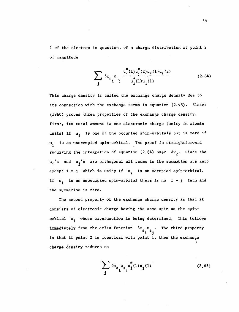
34
1 of the electron in question, of a charge distribution at point 2
of magnitude
ui(l)u (2)u (l)u. (2)6m m (2.64)6msim u Ui(l)ui(l)j Ji i u Mu (1)
This charge density is called the exchange charge density due to
its connection with the exchange terms in equation (2.63). Slater
(1960) proves three properties of the exchange charge density.
First, its total amount is one electronic charge (unity in atomic
units) if ui is one of the occupied spin-orbitals but is zero if
ui
is an unoccupied spin-orbital. The proof is straightforward
requiring the integration of equation (2.64) over dv2. Since the
u. 's and uj's are orthogonal all terms in the summation are zero
except i = j which is unity if ui is an occupied spin-orbital.
If ui is an unoccupied spin-orbital there is no i = j term and
the summation is zero.
The second property of the exchange charge density is that it
consists of electronic charge having the same spin as the spin-
orbital ui whose wavefunction is being determined. This follows
immediately from the delta function 6ms m . The third propertyii
is that if point 2 is identical with point 1, then the exchange
charge density reduces to
6ms
ms uj(l)uj(1) (2.65)Si Sij
35
or the total density of all electrons of the same spin as the ith
at position 1. These three properties allow the general nature of
the exchange charge density and its physical significance to be
determined.
Thus, the Hartree-Fock equations, as written in equation (2.63),
show that the potential energy of the field in which the electron
moves is the potential due to the nuclei plus the potential from
all electrons of spin opposite to that of the electron under con-
sideration, plus the potential from a charge distribution of
electrons of the same spin as the electron under consideration and
equal to the total charge of these electrons,minus the exchange
charge density. The charge distribution of electrons of the same
spin as the one considered adds up to one less than the total
number of electrons of this spin for an occupied orbital and it
includes all the electrons of that spin for an unoccupied orbital.
For the occupied orbitals, the net charge density of electrons
having the same spin as the electron under consideration, when
corrected for the exchange charge, goes to zero at point 1 where
the electron under consideration is located since when point 2
coincides with point 1 the exchange charge density cancels the
total density of all electrons of this same spin. In other words
the electron tends to keep other electrons, having the same spin
as it, away. Thus the effect of the exchange terms is to remove
electronic charge from the immediate vicinity of the electron
whose wave function is being considered. This removal is more
36
effective with the Hartree-Fock method than with Hartree's
original method. This has the effect of lowering the potential
energy in the Hartree-Fock method so that it is expected that the
one-electron energy parameter ei = Aii would be lower in the
Hartree-Fock method than the Hartree method. This lowering of
the potential energy may also have an appreciable effect on the
wavefunction. Such an effect is observed in that the Hartree-
Fock equations, as compared to the Hartree equations, concentrate
the charge density more at small values of r (Slater, 1960).
Equation (2.60) has N solutions representing the N spin-
orbitals occupied in the determinantal wavefunction which repre-
sents the state of the N electron atom. An infinite number of
solutions to equation (2.60) can be found which represent the
unoccupied spin-orbitals. It has also been shown (Slater, 1960)
that all solutions of the Hartree-Fock equations are orthogonal
and when normalized they form a complete set of orthogonal spin-
orbitals in terms of which an arbitrary function of coordinates
and spin may be expanded. The above results (except for the
unitary transformation for the Xij's) do not depend on the fact
that a central field problem (or a closed shells) is being
considered but only on the fact that a determinantal wavefunction
is being used. Energies are found in this approximation by solving
equation (2.60) numerically and calculating Havg
It was first pointed out by D9lbruck (1930) and later proven
more explicitly by Roothaan (1951) using group theory, that for
an atom which has all of its electrons in closed (completely
37
filled) shells the Hartree-Fock one-electron orbitals ui must
have the form of solutions of a central-field problem so a single
determinant is appropriate. For this case Hartree's assumption
of a spherical average is not necessary as the spherical behavior
necessary for using the solution u. comes about automatically.
For nonclosed shells this is not the case and a spherically
averaging process must be carried out in order to get one electron
orbitals of the central field type. This procedure has been
carried out (Brown, 1933; Hartree and Hartree, 1935; see Slater,
1960, for a discussion of this point) and is shown to be the
result of Just the variation of the radial part of the one electron
orbitals (exactly as outlined in the above discussion). The two-
electron integrals are however much more complicated for unfilled
shells (and when a spherical average is not performed as in the
simple Hartree case) (see Slater 1960 p. 310). Thus the best solu-
tions of the spherically symmetric problem are obtained even when it
is not actually spherically symmetric (i.e., the u.'s are not really
appropriate). This is however, a good approximation since in most
cases the potential is almost spherically symmetric. The Hartree-
Fock procedure requires a considerable amount of computational time
as each term (L and S specified) of a given configuration requires
a separate calculation and it has only been through the use of
electronic computer that other than simple problems can be handled.
38
E. Calculations
The calculations of the Hartree-Fock wavefunctions for this
investigation were carried out with the Hartree-Fock computer pro-
gram developed by C. Froese (Fischer) (1965) on the C.D.C. 6600
computer at NASA's Langley Research Center, Hampton, Virginia.
This program calculates the spin-orbital functions, the total
energy of the term, as well as the radial spin-orbit interaction
parameter
Cng = Pnf(r) )P(r) dr (2.66)
where i(r) is defined in section A.
The program also employs the configuration interaction
representation which is an extension of the Hartree-Fock method.
In this representation the total wavefunction is expanded in terms
of the determinantal wavefunctions associated with more than one
configuration although for the calculations performed this repre-
sentation was not needed.
Initial estimates of the term energy, wavefunction and the
initial slope of the wavefunction were obtained from the Hartree-
Fock-Slater program of Herman and Skillman (1963) which employs
a modified Hartree-Fock.procedure with the exchange potentials
for different occupied orbitals replaced by a universal exchange
potential formed by using an exchange charge density taken from
39
the case of a free-electron gas. The exchange correction is then
written as a constant multiplied by the cube root of the change
density and therefore eliminates the necessity of computing an
integral from the exchange charge density (Slater, 1951). The
program also employs a single determinantal wavefunction built up
of the one-electron spin orbitals. Furthermore, multiplet structure
is ignored so that the energy obtained from the wavefunction is
just an average energy of the configuration. These results,
however, do make very good initial estimates for the more compli-
cated Hartree-Fock program.
The wavefunctions obtained from the Hartree-Fock program were
punched onto data cards and were employed to calculate the transi-
tion probabilities of the doubly excited states of interest.
The transition probability between an upper level with total angular
momentum J and a lower level with total angular momentum 1' is
given by (Garstang, 1969)
2.677 x 10⁹ (EJJ,)3S -
A(J + J') = + 1 sec (2. 67)
where EJ, is the energy difference of the levels in Rydbergs,
S is the absolute line strength for electric dipole radiation in
atomic units
sl/2(SLJ - S'L'J') = [(2J + 1)(2J' + l)]l/2W(L3L'J':Sl)(L lr(1) IL')6SS,
(2.68)
40
for a transition from the level SLJ to the level S'L'J'. W
is a Racah coefficient and the matrix element of the first order
tensor r(1) is in reduced form. The reduced matrix element of
the first order tensor r(1 ) may be evaluated in terms of the
one-electron wavefunctions (Shore and Menzel, 1965).
M , ,k +1-kl-L 1/2 1/2( 1 22L Ir()I l )1Z2L) = (-1) (2L + 1)1 / 2 (2L' + 1) 26 2P2
(n)/(rn {i t n-1) x W(o1Lf1L ;u21)(v1er (1)e l) (2.69)
where n is the number of equivalent electrons (n = 1 for no
equivalent electrons) and (kn{|l1 n-1) is the coefficient of frac-
tional parentage. For two equivalent electrons the coefficient of
fractional parentage is unity. This is the only possibility for the
case being considered (two electron ions). The reduced one-electron
matrix element has only two nonzero values (Garstang, 1969)
( Ir(l) I+ ) - [( + + 1) + (2 + 1)(2 + 3)11/20
(2.70)
and
(kIIr(1)Ik - 1) = + [<(2k - l)(2 + 1) /2 (2.71)
41
with
(4 2 1)/2 rPn(r)P,,(r')dr (2.72)
where k is the greater of the two V's involved in the integral.
The Hartree-Fock wavefunctions were employed to numerically evaluate
the integral in equation (2.72) using a computer program developed
by Shamey (1970). The absorption oscillator strength f(J' - J)
is given in terms of the absolute line strength by (Aller, 1963)
f(J',J) = 303.7 S(SLJ - S'L'J') (2.73)
where X is the wavelength in Angstron unit. The quantity g
(g = 2J' + 1) is the statistical weight of the lower state and
g f(J:J) is often the quantity tabulated.
The numerical calculations indicate that the three ions of
interest are in good LS coupling since the spin-orbit splitting
of the terms was very small compared to the separation of the
terms.
The wavefunctions and total energies of the ground state,
singly excited and doubly excited states of the two-electron ions,
boron IV, carbon V, and nitrogen VI were calculated with the
Hartree-Fock program and the energy difference between terms for
which electron dipole transitions were allowed was converted
to wavelengths. Terms rather than levels were used since all levels
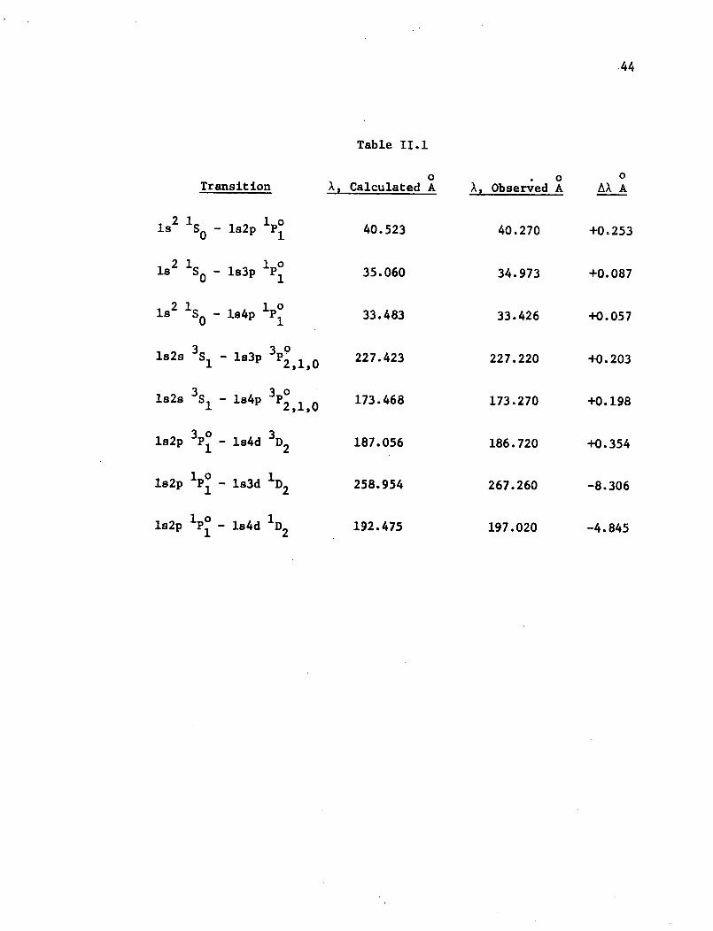
42
in a given term were assigned the same energy. In order to deter-
mine an order of magnitude error involved in the calculated wave-
lengths the energies of the singly excited states and ground state
were used to calculate wavelengths of observed transitions in the
two-electron ions of interest. These calculated values are compared
with the observed values in table II.1. The observed values are
taken from the listing of Kelly (1968). The calculated wave-
lengths are generally in very good agreement (< 0.5 percent error)
with the observed values with the exception of transitions having
lsnd 1D as an upper term where the error is much larger (up to
about 3 percent). The calculated wavelengths were in sufficiently
good agreement with the observed values that including the effects
of configuration interaction would not improve the agreement
sufficiently to justify the rather large amount of labor involved.
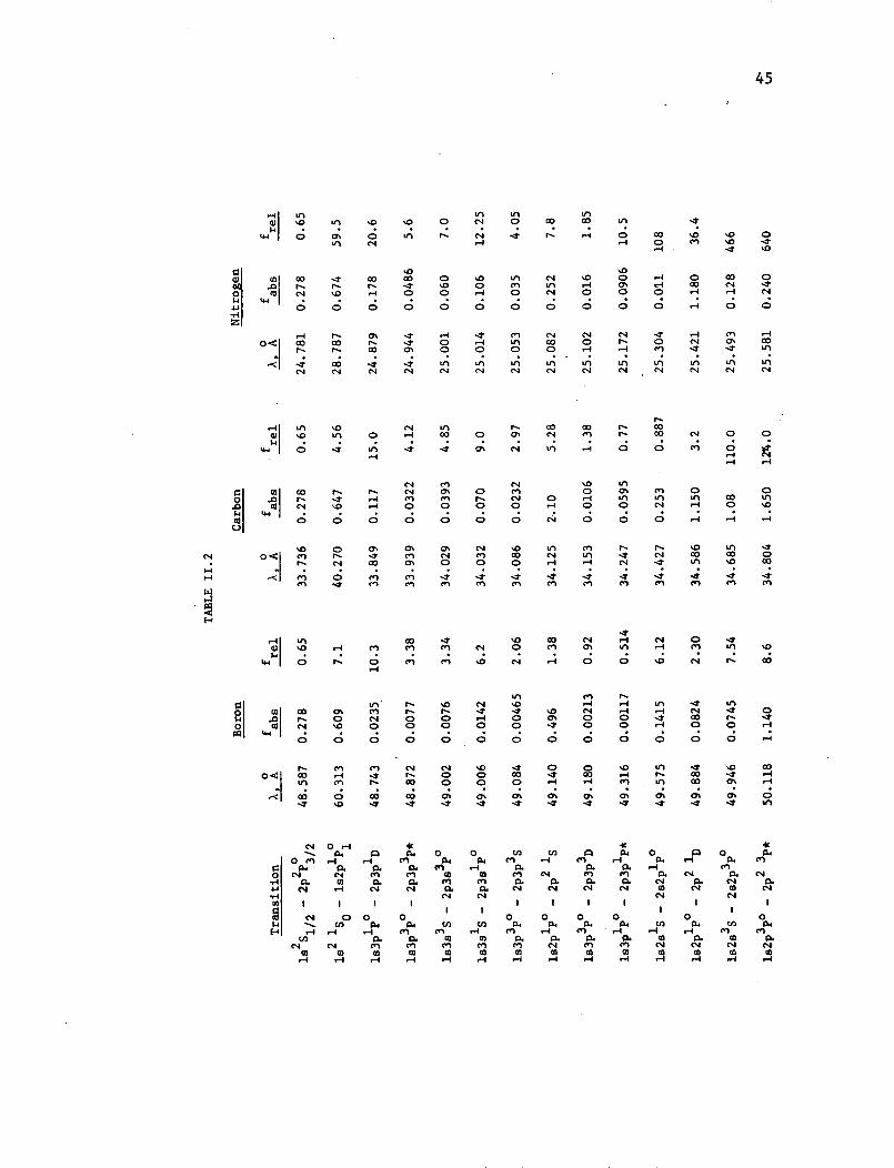
Wavelengths of electric dipole transition between the doubly excited
and singly excited terms were then calculated in the above manner.
The transition, wavelength, calculated absolute f value, and
relative f value in the multiplet, are listed in table II.2.
The wavelength, absolute f value, and relative f value for the
hydrogen-like and helium-like resonance lines of each ion are also
listed. While the calculated energy difference of the various
terms of the singly excited states agrees rather well with the
observed values, this is not the case for the oscillator strengths
and resulting transition probabilities. The transition
43
probabilities for the helium-like resonance line is larger by a
factor of 1.6 for boron IV,up to a factor of 7 for nitrogen VI when
compared with the transition probabilities of Dalgarno and
Parkinson (1967). These authors obtained oscillator strengths
for the resonance transition of helium-like ion by expanding the
electric dipole matrix elements connecting the ls2 iS and ls2p 1p
states in inverse powers of the ionic charge Z. By comparing
their method with the Hartree-Fock approximation they find that
the matrix element which they obtain differs from the Hartree-
Fock approximation by one term which they regard as a virtual
dipole excitation of the passive ls electron plus a distortion
due to the dynamic polarization of the ls orbital at the is -
2p transition frequency. They further show the necessary correc-
tion to the Hartree-Fock approximation consists of mixing the
(ls2) S and (apnp) S configurations with ap representing the
polarized is orbital. Consequently, it is expected that the
calculated transition probabilities for the doubly excited states
are too large and are only accurate to an order of magnitude.
44
Transition
ls2 1S0 ls2p P1
2 1ols2 S - ls3p P1
ls2 1S0 - 14p 1p
3 0s2s 3S1 - ls3p P2,1,0
ls2s 3S1 - ls4p P2,1,0
ls2p 3 P1 - ls4d 3D2
ls2p P1 - ls3d 1D2
ls2p I -_ ls4d D2
Table II.1
0X, Calculated A
40.523
35.060
33.483
227.423
173.468
187.056
258.954
192.475
0 oX, Observed A AX A
40.270 +0.253
34.973 +0.087
33.426 +0.057
227.220 +0.203
173.270 +0.198
186.720 +0.354
267.260 -8.306
197.020 -4.845
In LAu, 5 O so 0 e 0 co(;, 8 9 4 4 9~vIn C4 I-fa
a
. 1~~~~c0 C* s,o 0 cn
H
j osO
o0 H 0
6 q o
J0*
O ,l O O'0 0 . LA
O H 0 O
O O O Oeq
o o t 0c
'0'0 O -4 0
O 0 H-4
o o 0 o H
Ln Ln Ln LU
,-I ,- c, ~
c~4 ~4 ~ 0
LU o H- LA -
H
00n~ O c4 *5 00 c~~~ -LA N- co co 0 - coCO 0o O L n H 0 C
0 .0 N-.0 co eq
.4 4-4
s0
H .
H LA
) O
eq
0o 0 oCl Cl
09_4 c;H O ClC- 0 ClH~o
cnoa 0m r-o 0
0%
o o
J -tIn en
oq 00 H
o J
o 0 H LA Ln LA
o 0 H-48 8 8 4
'0 CL C. r- OO H H , -- LA
-t -e m en -tCl C Cl Cl l C
- o 0 cc H , - e Ocn Cq 0 o n 05 LA H ClA 1 C4 6 1t c-
0
0 \o
co 0
J .en cP
.-LA so1C- CO
%O Cn O-
O O O
sO ce
O Ho 0
O O
LUsO
O -Oo 0O O
H H LA 4
O O H O0
8 6 8
r- CnCVO H
CO 0
t I_- co
T -T
O 50o 0
0% 0%1; a
'CO -O 0 H - coo H H c- LA CO
- ,- , - st ti
ro CO
% 0er A
_ . Q 0 04 tX "O
0 H H n PA P4 <n l n .4 H P4 cO. 0 0. C H . 0. 0. H C ,
0 C1- C-4 n c 0 1 c . en 0. - 0. C04H C . 0o 0. 0. Cl l 0.i 0. 0. 0. c'J 0. C- p,
1 4 H n c. 0. eq eq ( cs eq C e e
Co I I I I I I I I I I
-4 - -4 P4 A CA P4 P4 P4 P4 -P C
cH 000 0 0 00 0 H '~ cnm aa mm
N ~ ~ Cw ~n u~ ~w ~w cu ~w n cn P,-¢ -¢ .- ¢ ~ . . .Im,- ~',I ,"~ ,.4 '
45
4-4 0
toco
04
I< -T
eq
0 00D -t
-t sO
,4l v
o 0
0 0
o 0
O. CO
LA LACS r4
o o
H .1-4 1-
C o 0 N0 co -
-T 0O
4 -4O HO H
CHAPTER III
Atomic Processes and Plasma Models
A. Ionization Processes and Rate Equations
For many astrophysical as well as laboratory plasmas, thermody-
namic equilibrium is never achieved and, consequently, an analysis
of the emitted radiation requires a knowledge of the rates at which
the various atomic processes take place. The rates of ionization
and recombination as well as the population and depopulation of the
various atomic states are of importance.
Let XZ-l(p) and XZ(i) denote two successive stages of
ionization of an atom X with number density nZ-l(p) and nZ(i)
-3per cm . The superscript Z - 1, Z represents the ionic charge
of the atom and the ionization potential of the pth state of XZ- 1
2is denoted by Ip(Ip = - EH for hydrogenic ions). The letters
Pp or i represent an arbitrary level of the atom with statis-
tical weight g(p), g(i). Free electrons e, having number density
-3n cm are also present in the plasma and a radiation field of
intensity I(v) at the frequency V may also be present. The
reversible process
X- (p)+ X (i) + e (3.1)
with the left to right process ionization and the right to left
processes recombination may now be considered. Ionization by elec-
tron collisions
47
XZ -l(p) + XZ(i) + e + e (3.2)
has as its inverse three body recombinations. If K(p,c) is the
rate coefficient for collisional ionization then the rate at which
ionization takes place is
nen (p)K(p,c)cm sec (3.3)
and the rate at which three body recombination takes place is
n2nZ(i)K(c,p)cm sec-1 (3.4)e
The rate coefficient K(p,c) has been evaluated by Jefferies
(1968) using an expression due to Fowler (1955), a Maxwellian
velocity distribution for the free electrons and a dipole approxi-
mation cross section for the process derived by Seaton (1962).
Those approximations, although quite crude, will be sufficient
for the investigation considered here. He obtains the relation
(in cgs units)
Kp,'1 11 A(P )T/2
K(p,c) - 1.55 x 10³ exp (-Ip/kTe)cm sec (3,5)p
where A(p) is the photoionization absorption cross section at
threshold of the level p, gi is a scaling factor whose value
depends on the charge of the atom (gi = 0.3 for Z - 1 > 2) and
T is the electron temperature in OK.e
48
The rate coefficient for three body recombination K(c,p) is
related to the rate coefficient for collisional ionization K(p,c)
by the relationship (Jefferies, 1968)
K(c,p) = 2.06 x 10 -16 (p3/2 exp (-Ip/kTe)cm sec (3.6)UZ(Te)Te3/2 p e
where UZ(Te) is the partition function of the atom XZ and the
free electrons have a Maxwellian velocity distribution. Because of
the dependence of I on p2 and the statistical weight g(p),P
K(c,p) may become very large near the series limit. The inverse
temperature dependence will cause K(c,p) to decrease with increas-
ing temperature, so that, for recombination into the first few
excited levels of an atom at very high temperature the rate co-
efficient should be small.
Photoionization may also occur with its inverse, radiative
recombination
Xz1(p) + hv XZ(i) + e (3.7)
where hv represents a photon of frequency v. The rate of photo-
ionization is
n (p)R(p,c)cm -3sec (3. 8)
49
where the rate coefficient R(p,c) is (Jefferies 1968)
R(p,c) = 4r I(f V V)dv % sec-1 (39)hV
vo
The absorption coefficient ca() at the frequency v is related
to the optical depth T(V) (Cooper, 1966)
dT(v) = - a(v)dx (3.10)
where dx is an element of length along the line of sight. Plasmas
for which T(v) << 1 are called optically thin at the frequency v
while those for which T(V) > 1 are referred to as optically thick
at the frequency v. Photoionization is therefore unimportant in
optically thin plasmas as a photon will not be absorbed.
The rate at which the inverse process, radiative recombination,
into the level p occurs is
nen (i)R(c,p)cm -3sec (3.11)
The rate coefficient into a hydrogenic level p having a photo-
ionization cross section A(p) and a threshold ionization energy
I is (Seaton 1959)
R(c,p) = 3/2 exp(Ip/kTe) (h\))A(p)exp(- e )d(v)cm 3sec
c Tr (mkTe) Ip/kTep
(3.12)
50
Radiative recombination depends on the electron temperature but its
inverse does not.
In multi-electron atoms or ions doubly excited states having
energies above the first ionization potential of the atom or ion
are possible. These doubly excited states, subject to certain
selection rules, may undergo a radiationless transition
XZ-1 (d) X(i) + e (3.13)
where d represents the doubly excited state. This process is
known as autoionization and the selection rules are just those pre-
viously discussed for matrix elements of the operator H1 to be
non-zero, that is, the two states [right and left side of equation
(3.1)] must have the same total angular momentum J (in LS
coupling the same L and S), the same parity and the same energy
E. The rate at which autoionization occurs is
nZ- (d)Aa(d,c)cm3se
- 1(3.14)
where Aa(d,c) in the autoionization transition probability. The
transition probability may often be quite high (~1013 - 1014 sec )
(Cooper 1966). The inverse process (right to left in equation (3.1))
is called inverse autoionization and occurs at a rate
nn Z(i)A (c,d)cm-3sec (3.15)e
51
The movement of the electron from the continuum to the discrete
doubly excited state leads to a transient recombination since auto-
ionization maintains a quasi-equilibrium in which the number
density of doubly excited states n Z-(d) is small. If true re-
combination is to occur the doubly excited states must become immune
to autoionization. Therefore it is necessary to discuss the pro-
cess by which excited states (either singly or doubly excited) are
formed and de-excited.
B. Bound-Bound Transitions and Rate Equations
An atom of charge Z having energy levels p,q with statistical
weights g(p), g(q), an energy separation E(p,q), absorption
oscillator strength f(p,q), and with the level p lying below q
is considered. The index q may be either a doubly-excited or a
singly excited level and p then represents either a singly excited
or unexcited level (or a lower doubly excited level) respectively.
Electrons may be excited into a higher state by electron
collisions
nZ(p) + e nZ(q) + e (3.16)
at a rate
Z -3 -1 (3.17)nn n (p)K(p,q)cm sec (3.17)e
52
In high-temperature plasmas the excitation of ions rather than
neutral atoms is important. An expression for the excitation of
ions has been derived by Seaton (1962) in the Born approximation
K(pq) = 6.5 x 10 -4
3 -K(p,q) =1/2 f(p,q)exp( - E(p,q)/kT e)cmsec (3.18)
E(p,q)Te
The inverse process is collisional de-excitation and is just the
right to left process of equation (3.16). The rate at which
collisional de-excitation from the level q to the level p occurs
is
nen (q)K(q,p)cm -3sec 1 (3.19)
where the collisional de-excitation coefficient K(q,p) is related
to the excitation coefficient by (McWhirter, 1965)
K(q,p) = (-) K(p,q)exp(E(p,q)/kTe)cm3sec (3.20)g(q)e
If a radiation field is present in the plasma, photoexcitation
will occur if the plasma is not optically thin
XZ(p) + hU + XZ(q) (3.21)
The rate at which this photoexcitation takes place is
(Jefferies, 1968)
53
n (p)I(V)B(p,q)cm sec (3-22)
where I(v) is the intensity of the radiation field at the fre-
quency v and B(p,q) is the Einstein transition probability for
absorption. The inverse process of photoexcitation is radiative
de-excitation
XZ(q) + XZ(p) + hv (3.23)
and is actually two processes, spontaneous emission with a rate
nZ s~n~g~p~cm-3 -1
nZ(q)A(q,p)cm sec (3.24)
and stimulated emission with a rate
n (q)B(q,p)I(V)cm 3sec (3-25)
In practice, stimulated emission is treated as negative
absorption so that the two processes which depend on the intensity
of the radiation field are lumped together as a single process
with a single rate coefficient.
C. Doubly Excited States and Dielectronic Recombination
The two step process consisting of inverse autoionization to
form the doubly excited state followed by radiative decay of the
54
doubly excited state to a singly excited state is called dielectronic
recombination and is the process of interest in this investigation
since the radiative decay of the doubly excited state in a two
electron atom will produce a photon that is of a slightly lower
energy than the corresponding transition in the one electron atom
and should therefore produce satellites to the hydrogen-like lines.
If the probability of a radiative transition from the doubly excited
state to a lower stable state is AS(d,p) then the rate at which
the doubly excited state is depopulated by this process is
n (d)A (d,p)cm sec (3-26)
The rate coefficient for dielectronic recombination is denoted
by Kd(c,p) and the rate at which dielectronic recombination occurs
is (Bates and Dalgarno, 1962)
nnZ (i)Kd (c,p) (3-27)
Figure 1 is a schematic of the various processes involved in
dielectronic recombination and is useful in determining an expression
for Kd(c,p). The processes are:
#1. Spontaneous decay - rate given by equation (3.24)
#2. Autoionization - rate given by equation (3.14)
#3. Inverse Autoionization - rate given by equation (3.15)
Equating the rate into the doubly excited state with the rate out of
the state
55
n Z-(d)[A (d,p) + Aa(d,c)] = nn ZAa(c,d) . (3.28)
The coefficient for inverse autoionization may be related to
the equilibrium value of n Z-(d) by detail balance and using
full thermodynamic equilibrium.
Thus
nZ-l(d)Aa(d,c) = nenZAa(c,d) . (3.29)
Substituting for n nZAa(c,d) in equation (3.28)
nZ (d) = nZ (d Aa
(d,c) cm- 3 (3.30)-E (d) Aa(d,c) + AS(d,p)
The rate of stabilization of the doubly excited state is given by
equation (3.26) and nE(d) is the number density in SAHA equili-
brium (which will be discussed in the next section). Equating
equation (3.27) with equation (3.26) (i.e. setting the rate of
dielectronic recombination equal to the rate of stabilization of
the doubly excited states)an expression for the rate coefficient
is obtained
ZlA\AsA~ 3 -1K (c,p) = n d)Asdp) cm sec (3.31)
nZ(i)ne
Z-11nE (d) Aa(d,c)AS(d,p) cm3Sec
n A c) + Adp)n(i)ne A (dc) + A (d,p)
56
where equation
expression for
becomes (Bates
(3.30) has been substituted for n -l(d). Using the
Saha equilibrium (see the next section) the expression
and Dalgarno, 1962)
Kd(cp) = A (d,c)AS(d,p)Aa(d,c) + AS(d,p)
g(d) h 3/2 exp {
2U (Te ) (27rmkTe ) 3/2e e
E. }(3.32)
kTe
where es is the amount of energy by which the doubly excited
state-exceeds that of the state (i). The state (i) is normally
taken to be the ground state.
The doubly excited state may also be collisionally de-excited
[equation (3.19)] and the conditions under which this is important
must be examined since if collisional de-excitation competes with
radiative the above arguments are no longer valid. The collisional
de-excitation rate coefficient for a state may be expressed in
terms of the lifetime of the state to radiative decay Tr(d,p)
(Bates and Dalgarno, 1962)
K (d,p) = b[10- 2
9 A4/Tr(d,p)]cm3 sec- 1
(3.33)
where the parameter b is a characteristic of the process and is
of order unity and X is the wavelength of the emitted phQton in
Angstroms. The lifetime of the doubly excited state toward
collisional de-excitation is (Bates and Dalgarno, 1962)
(3.34) -Tc(dp) =l/K6(dsp)ne seC.
57
Substituting in equation (3-33) the ratio of collisional to radia-
tive lifetime is obtained
c(d,'P) 102 9 /b A4nT (d~pT = 10 /b X n e (3.35)e
o 23The ratio becomes unity for X = 30 A and b = 1 if n = 1023
-3cm . Thus at high electron densities collisional stabilization
of the doubly excited states may become important. At the
electron densities encountered in this investigation (ne = 2.2 x 10¹⁷
cm ) stabilization by radiative decay should dominate. It should
not be concluded however, that collisional processes between the
doubly excited states are unimportant.
Processes involving atom-atom, atom-ion, and ion-ion collisions
have rates which are much smaller than those involving electron
collisions if the degree of ionization of the plasma exceeds a few
percent. These various processes have therefore been ignored as
their contribution would be extremely small.
D. Equilibrium Relationships and Detail Balance
If multielectron atoms are present in the plasma, more than one
stage of ionization is possible and the various processes must be
considered in and between the various stages. The general procedure
to obtain the population density of the various quantum states
consists of setting up the rate equations for the various processes
58
which have been discussed and solving them simultaneously. In
general, this is a laborious and time-consuming job and, in many
cases, a complete solution is impossible to obtain due to the number
of states involved. In complete thermodynamic equilibrium, each of
the processes discussed is just balanced by its inverse. In other
words, the pairs of processes occur in detailed balance. In this
situation, the distribution between two stages of ionization nZ
Z-1and n is given by Saha's equation
n nZ r mkT 3/2 UZ(T
e =2 e 2 e exp (- E /kTe) (3.36)nZ-1 h2 UZ-_(Te)
where the U(Te)'s are the partition functions of the two atoms or
Z-1 Z-1ions and £ is the ionization potential of the atoms n
The population density of the state q of the ion nZ is related
to the total number density of nZ by the Maxwell-Boltzmann equation
(Cooper, 1966).
nZ(q) = gLq) exp (- E(q,p)/kTe) (3.37)n UZ(Te)
Furthermore, the free electrons have a Maxwellian velocity distri-
bution and all distributions are characterized by a single temperature
T.
In astrophysical and laboratory plasmas, complete thermodynamic
equilibrium is almost never obtained. There are, however, two
59
regimes where useful approximations can be made. If the plasma den-
sity is sufficiently high, then collisional effects will completely
dominate radiative effects and detail balance will be obtained
between the collisional rates. The distribution of electrons among
the various energy levels is the same as it would be if the system
were in complete thermodynamic equilibrium. Although the plasma
temperature and density may vary in space and time, the distribution
of electrons (both bound and free) depends entirely on local values
of temperature, density, and chemical composition of the plasma,
and hence this regime is called local thermodynamic equilibrium (LTE).
In plasmas, this equilibrium is characterized by the electron
temperature Te, since it is the electrons which dominate the
collisional processes. In order for radiative decay rates to cause
less than a 10 percent departure from LTE, the collisional rates
must be at least about 10 times the radiative rates (McWhirter, 1965).
This problem has been considered in detail by Wilson (1962), Griem
(1963), and McWhirter (1965). Each of these authors arrived at
essentially the same expression for the electron density required
for the collisional de-excitation rates to exceed the radiative
decay rate of a particular level with excitation energy E(p,q) by
a factor of 10, namely
1
n > C T E3(p,q) cm (3.38)e- e
60
The three authors arrive at different values for the constant
C although all three values agree to within a factor of 2. The
values of C are 9.2 x 10¹¹ (Griem), 1.3 x 10¹² (Wilson), and
1.6 x 10¹² (McWhirter). The inequality expressed in equation (3.38)
is a necessary but not a sufficient condition for a plasma to be
in LTE. The necessary and sufficient condition for the plasma to
be in LTE requires in addition that the lifetime of the plasma
exceed the relaxation time of the slowest collisional processes of
importance (Griem 1964). This condition is often not fulfilled in
laboratory plasmas.
If the plasma density is sufficiently low, radiative rates be-
come important and may dominate some of the collisional processes.
If the plasma is also optically thin, collisional ionization and
excitation may be balanced by radiative and dielectronic (although
this term was not originally included) recombination and spontaneous
decay. This is the model which has been proposed to explain some
features of the solar corona (Wooley and Stibbs, 1953; Elwert,
1952) and is often referred to as the coronal approximation. The
state of ionization in a plasma in coronal equilibrium is determined
by balance between collisional ionization from the ground state and
radiative and dielectronic recombination. Radiative recombination
into all levels is included, since recombination into an excited
level is immediately followed by spontaneous emission to a lower
level. Since the total transition probability
A(q) = E A(q,p) (3.39)
p<q
61
from the excited level q is large (at least if q is not too large
as there will always be some q for which this is not true), the
lifetime of the state toward radiative decay is small (T = A (q)).
If the time between collision is longer than the lifetime of the
level (e.g., low density plasma) collisional excitation from the
ground state only needs to be considered, since the population of
the excited levels will be small. At equilibrium
nen (l)K(lc) =nen (1) [R(c,p) +Kd(C,p)] (3.40)
so that
n (1) K(l,c) (3.41)
nZ- (1) [R(c,p) +Kdc,pP)]
which is independent of the electron density and is a function of
electron temperature only. The ratio n /nz-1 depends critically
on the cross sections for the processes so that the accuracy of
the calculated values of the ratio will be determined by the accuracy
of the cross section used.
Post (1961) has calculated relative abundances of some common
impurity ions in laboratory plasmas using approximate cross sections
for hydrogenic (one electron) and lithium-like (three electron)
ions. His results indicate that Saha's equation does not accurately
predict the ratio n /nZ- 1
in the coronal regime and that at
extremely high temperatures heavy ions may exist without being
62
completely ionized. A comparison of the population density of
carbon ions calculated by the two methods for a density of n =
1017 cm-3
is shown in figure 2.
It has been pointed out by Burgess (1965a) that under certain
conditions, dielectronic recombination may compete with and may
even exceed the rate of radiative recombination (which was included
in equations (3.40) and (3.41)). Post's calculations did not
include dielectronic recombination.
Since collisional excitation and collisional ionization from
the ground state only is consistent with the coronal model, the
population density of the excited states of a species is obtained
by the balance between collisional excitation and radiative decay
(Cooper, 1966).
n (q)A(q) = n (l)neK(l,q) (3. 42)
Then,
n(q) neK(lq)n(l) A(q) (343)
The rate coefficients K(l,q) [equation (3.18)] are, in general,
strongly dependent on the electron temperature. Since n(q) << n(l)
is required with 'the coronal model, these values must be investi-
gated by the substitution of known or estimated values.
63
E. Application to Laboratory Plasmas
The coronal model has been discussed in the context of a steady-
state plasma in which it was assumed that changes in the population
densities of the energy levels caused by variations in the electron
temperature or density take place at a rate that is slow relative
to the rate of relaxation of the atomic processes. The application
of such a steady-state model to the analysis of pulsed high-
temperature laboratory plasmas leads to the result that the plasma
lifetime in the device is shorter or about the same as the relaxa-
tion times for the various dominant atomic processes (McWhirter,
1960). It is therefore important to consider a time-dependent
model to describe such laboratory plasmas.
In a time-dependent coronal model, the spectrum is no longer a
unique function of the local conditions in the plasma but will
depend on the past history of the density, temperature, and state
of ionization of the plasma. Mathematically, this means that a set
of differential equations must be solved to predict the spectrum.
If the plasma temperature and density vary with time as they cer-
tainly do in pulsed laboratory plasmas, the rate coefficient in the
differential equation will also vary with time. Some assumptions
must be made in order to apply such a model, including the
assumption that the free electrons interchange energy at a suffi-
ciently rapid rate by both elastic and inelastic collisions so that
despite the changing conditions in the plasma, the velocity
distribution is always closely Maxwellian. The same processes which
·64
dominate in the steady-state corona model are also assumed to
dominate in the time-dependent model (i.e,, excitation and ioniza-
tion by electron collisions and de-excitation and recombination by
radiative decay and radiative and dielectronic recombination, respectively).
These processes are not instantaneous, and therefore the bound electrons
have a finite relaxation time into the new population distribution.
This relaxation time is controlled by the slowest processes that
influence the population distribution. These processes are the
slowest ionization or recombination rates which are determined by
the coefficients for the last ion to be produced in the plasma
(Goldman and Kilb 1964, McWhirter 1965). For an ionizing plasma,
this is the ion of greatest charge, and for a recombining plasma
the ion of least charge.
The validity of such a time-dependent model is determined by
how well it predicts the time history of line radiation from the
various stages of ionization in a plasma with rapidly changing
density and temperature. The power radiated per unit volume per
unit solid angle per unit frequency interval is
e(v) = h-v 4(v)A(q,p)n(q) (3.44)47T
where ¢(v) is the line profile and is normalized such that
J *(v)dv = 1 (3.45)line
65
The total power radiated in the line per unit solid angle is
hvT = 4- A(q,p)n(q) (3. 46)
For a plasma in coronal equilibrium, the intensity of a line is
(McWhirter, 1965)
I(qp K(1,q) A(q,l)ds (3.47)I(q,p) e A(q)
where equation (3.43) has been inserted for n(q) and the inte-
gration is over the depth of plasma viewed by the detector and it
has been assumed that the excited states are instantaneously in
equilibrium with the ground state. For a pulsed laboratory plasma,
ne, n(l) and K(l,q) may all vary with time, and it has also been
pointed out (Burton and Wilson, 1961) that the total number of
particles is not conserved due to escape of the plasma as well as
injection of atoms from the walls of the confining vessel. However,
McWhirter (1965) shows that if temperature and density vary compara-
tively slowly, the excited level population establishes itself
in a time which is just equal to the reciprocal of A(q)(i.e., the
lifetime of the excited level against radiative decay), and that
under these conditions the line intensity is given by equation (3.47),
because the excited state population is in equilibrium with the
ground state.
Investigations of the time dependency of line radiation have
been conducted on several pulsed laboratory devices, including the
66
toroidal pinch (Burton and Wilson, 1961; Hobbs, et al., 1965) and
the linear theta pinch (Goldman and Kilb, 1964; Kolb and McWhirter,
1964). These investigations verified that the time-dependent
approximation could be successfully applied to laboratory plasmas
of short lifetimes. Furthermore, the work of Goldman and Kilb
(1964) and Kolb and McWhirter (1964) showed the applicability of
this type of model to the high-temperature plasmas produced in
theta pinches of the type employed in this investigation.
This investigation is concerned with the detectability of
radiation emitted in transition from doubly excited states [equation
(3.26)] and particularly if the satellite lines observed in theta
pinch plasmas could be due to those transitions with the doubly
excited state being formed by dielectronic recombination. The
number of doubly excited states which could in principle exist in
multielectron atoms or ions becomes exceedingly large as the number
of electrons increases. For this reason, the simplest case was
chosen for which doubly excited states could be formed [i.e., a two-
electron (helium-like) ion]. If the doubly excited state is formed
by inverse autoionization, then the rate at which they are formed
[equation (3.15)] will depend on the number density of one-electron
(hydrogen-like) ions available. The intensity of the satellite line
must also be compared to a known, easily detectable line in order
to determine the feasibility of detecting the line. For this
purpose, the resonance line of the hydrogen-like ion
67
ls2 - 2p P3/2 (3.48)
was chosen. The satellite line would then correspond to a transi-
tion of the type
is ni - 2p nk (3.49)
with the prominent satellites due to n = 2. The upper state will
consist of two equivalent electrons for n = 2 and k = p. This
does not lead to any major problems but the equivalence of electrons
must be taken into account in the calculation. The presence of the
additional electron reduces the field in which the transition takes
place, consequently reducing the energy of the transition causing
the spectral line to be slightly shifted to the long wavelength
side of the hydrogen-like resonance line. Satellites due to n = 3
move closer to and become merged with the resonance line so that
they become undetectable. The elements which were investigated
were chosen on the basis that the temperature and density in the
theta pinch plasma be compatible with the existence of the desired
stages of ionization as well as requiring that the elements be
easily introduced into the deuterium plasma. Furthermore, it was
required that the hydrogen-like resonance lines lie in an
accessible region of the spectrum. Three elements were found to be
compatible with the above requirements: boron, carbon, and nitrogen.
68
Since the coronal model (excluding doubly excited states) was
developed for plasmas of very low electron density, the applicability
of the model to the particular levels involved must be investigated.
This is necessary since the maximum electron density compatible with
this model is that density at which electron collisions start to
interfere with the assumption that the only mechanism by which the
excited level decays is spontaneous emission. The criterion of
applicability for the coronal model to the resonance transition is
then (McWhirter, 1965).
A(q) > n K(q,l) (3.50)
For the hydrogen-like resonance lines, q = 2 and A(q) = A(2,1).
The Einstein transition probability A(2,1) was calculated for the
three elements of interest using equation (2.67).[Equation (3.50)
would have to be modified slightly if doubly excited states are
included.] The collisional de-excitation rate was calculated from
equation (3.20) using an electron density of 2.2 x 1017 cm3 and
an electron temperature of 180 eV. The values of electron density
and temperature were experimentally determined and are discussed
in detail in Chapter IV. The results of these calculations are
presented in table III.1 and verify that, for the lines of interest,
the coronal model meets by a large margin the criteria of appli-
cability with respect to the electron density.
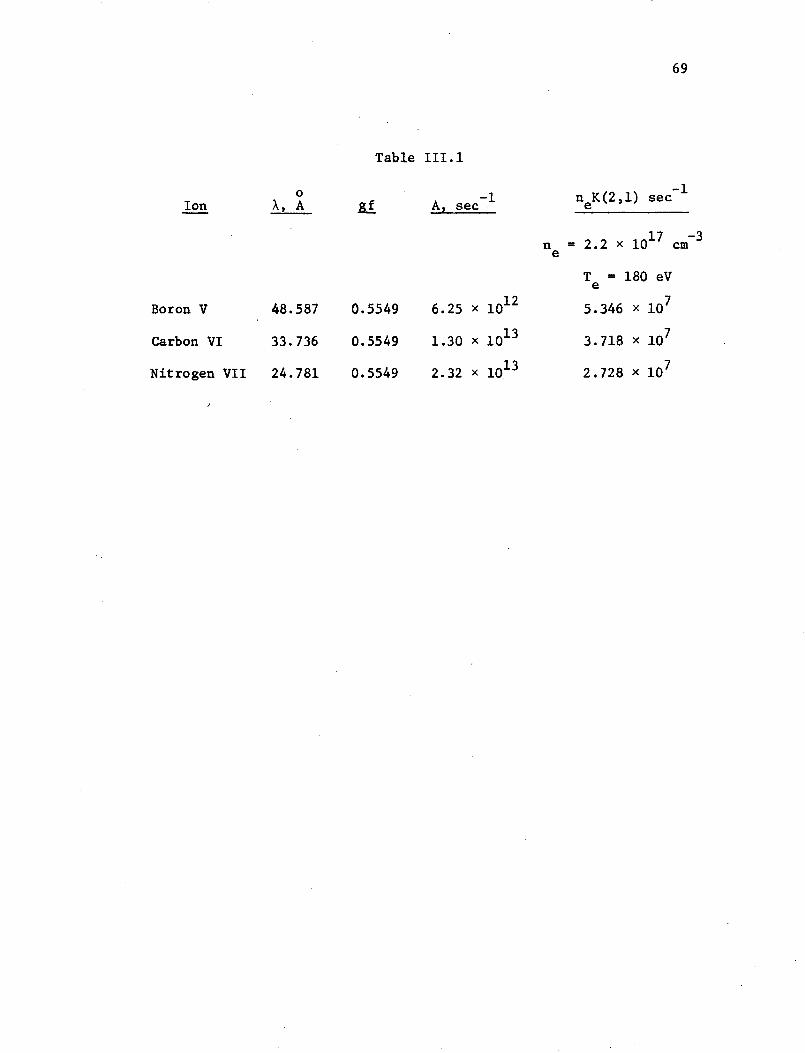
69
Table III.1
-1A, secn K(2,1) sec 1
e
Boron V
Carbon VI
Nitrogen VII
48.587
33.736
24.781
0.5549
0.5549
0.5549
6.25 x 10¹²
1.30 x 10¹³
2.32 x 10¹³
n = 2.2 x 1017 cm-3
T = 180 eVe
5.346 x 10⁷
3.718 x 10⁷
2.728 x 10⁷
Ion0
X, A
70
The intensities of the hydrogen-like resonance lines as well as
the intensities of the satellite lines play an important part in
this investigation, as the intensity ratio of the satellite to the
resonance line established the criteria to determine if the satel-
lites were, in fact, due to transitions from doubly excited states.
The intensity of a spectral line emitted by a plasma in coronal
equilibrium is given by equation (3.47) in the optically thin
approximation. Since this investigation is concerned with the
intensities of hydrogen-like resonance lines (Lyman-a) which are
large contributors to optical depth, the assumption of optically
thinness at the center of the resonance line which is needed for
the coronal approximation must be considered further.
The equation of radiative transfer may be written (Chandrasekhar,
1950) for a homogeneous plasma
dI(v) = - I(v) + (3.51)()dT(v) ct~v) (3.51)
where E(v) is the emission coefficient and a(v) is the absorp-
tion coefficient. In a uniform plasma e(v)/a(v) is independent
of the optical depth so that equation (3.51) has a simple solution
(Hearn, 1964)
I(v) = ( 1) [1 - exp ( - T(V)] (3.52)
For a line broadened by the Doppler effect
, . .
-,~~~~~ ;,,. -· . - . .' - ,. ,
71
T(V) = T(V o ) exp [ - (V - v )2 /(Av )2] (3.53)
where T(Vo) is the optical depth at the central frequency of the
line vo and Avo is the exp(-l) frequency of the Gaussian pro-
file. In a plasma close to LTE (i.e., collision dominated),
e(v)/a(v) is independent of frequency so that equation (3.52) may
be expanded and equation (3.53) substituted in the expansion.
Integrating the expression over frequency gives the total intensity
of the line (Burton and Wilson, 1961),
IT I(V)d= v ()o + .. .54)IT
t-21 2 3 (3.54)
Equation (3,54) shows that, for To very small, the total
intensity is linearly proportional to the optical depth or, that is,
to the total number of atoms. However, if T is 0.3, the total
intensity of the line is off by 10 percent from the linear relation.
Therefore, the optical depth must be restricted to less than 0.3 in
collision-dominated plasma if the optically thin approximation is
to be correct to 10 percent.
In the coronal model, radiative decay is much greater than
collisional de-excitation so that the population of excited levels
is determined by both collisional and radiative processes and the
criteria for optical depth must be re-examined. This case, applied
to the hydrogen-like resonance lines (Lyman-a), has been investigated
72
by Hearn (1964) using a model of the diffusion of resonance photons
in frequency space. The criteria for the validity of the optical
thin assumption are developed for Doppler-broadened resonance lines
on the basis of a two-level atom. The two-level atom gives a good
approximation to the Lyman-a line since the first excited level can
only decay radiatively to the ground level with the emission of a
resonance photon or it may be collisionally de-excited. The
probability b that the atom in an excited state will emit a
resonance photon is
b = + A(2,1)neK(2,1) + A(2,1) (3.55)
Of these photons, a fraction k will escape and (1
be absorbed, producing excited atoms. Of these excited
fraction b will emit resonance photons and a fraction
will escape. The total fraction W of photons emitted
of an original excitation is
- k) will
atoms, a
k of these
as the result
W = k + b(l - k)k + b (1 - k) k + . . .
k1 - b(l - k) (3.56)
The limiting optical depth for the approximation may be calcu-
lated for the value of k which is necessary to reduce W by, at
73
most, 10 percent. If W is set equal to 0.90 in equation (3.56)
the optically thin criteria becomes
k > k 0.90(1 - b) (3.57)min - 0.90 b
Calculated values of b and k are given in table 111.2min
for the resonance lines of interest and for the approximate plasma
condition under which they were observed. The value of k for the
plasma was estimated from the relation (Hearn, 1964).
k = 1 - .erAnT) 1/2 (3.58)
where erf is the error function. Equation (3.58) is applicable
if T > 1. The calculated values of k are listed in table III.20
with the values of b and k in. From table III.2 it is seen that
b is very close to unity and kin is quite small so that the
optically thin approximation for the total line intensity (not the
profile shape) based on the Hearn's (1964) model should be valid for
the lines investigated even though the optical depth calculated from
equation (3.10) with
~e2 F -1ac(v) n(p)f (p,q) 2cm (3.59)
mc 42 (2-v0
) + 2(4r (v 9 ) (2)
(Aller, 1963), for v = v and r = A(2,1)-
1 gives values of T0 o
for a length of 137 cm) of about 103 for concentrations of
5 percent impurity (boron, carbon,
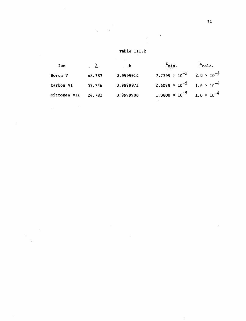
74
Table III.2
Ion
Boron V
Carbon VI
Nitrogen VII
48.587
33.736
24.781
b
0.9999914
0.9999971
0.9999988
min.
7.7399 x 10- 5
2.6099 x 10- 5
1.0800 x 10- 5
kcalc.
2.0 x 10⁻⁴
1.6 x 10⁻⁴
1.0 x 10⁻⁴
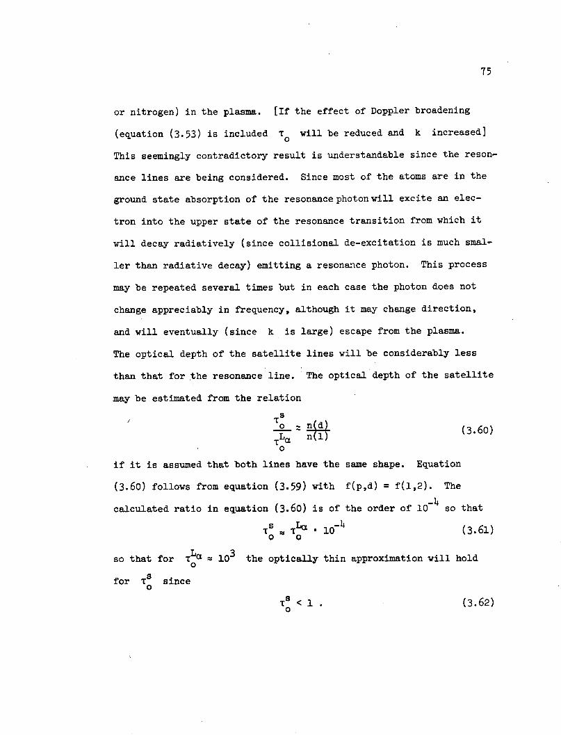
75
or nitrogen) in the plasma. [If the effect of Doppler broadening
(equation (3.53) is included T will be reduced and k increased]
This seemingly contradictory result is understandable since the reson-
ance lines are being considered. Since most of the atoms are in the
ground state absorption of the resonance photonwill excite an elec-
tron into the upper state of the resonance transition from which it
will decay radiatively (since collisional de-excitation is much smal-
ler than radiative decay) emitting a resonance photon. This process
may be repeated several times but in each case the photon does not
change appreciably in frequency, although it may change direction,
and will eventually (since k is large) escape from the plasma.
The optical depth of the satellite lines will be considerably less
than that for the resonance line. The optical depth of the satellite
may be estimated from the relation
T s
TLo. n 1(d)i0 nl)O
(3.60)
if it is assumed that both lines have the same shape. Equation
(3.60) follows from equation (3.59) with f(p,d) = f(1,2). The
calculated ratio in equation (3.60) is of the order of 10- 4
so that
Tso TL a 10
-(3.61)
0 0
so that for TL a t 103 the optically thin approximation will hold0
for Ts
since
0 O1 (3.62)
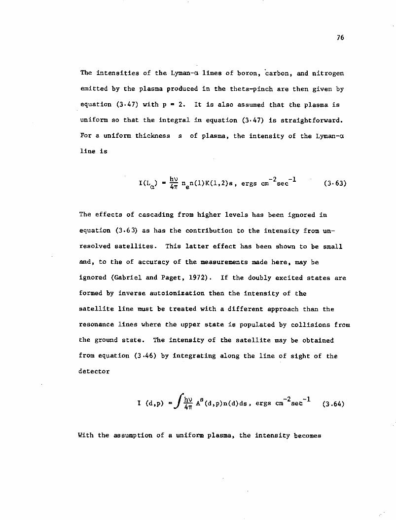
76
The intensities of the Lyman-a lines of boron, carbon, and nitrogen
emitted by the plasma produced in the theta-pinch are then given by
equation (3.47) with p = 2. It is also assumed that the plasma is
uniform so that the integral in equation (3.47) is straightforward.
For a uniform thickness s of plasma, the intensity of the Lyman-a
line is
hv -2 -1I(L ) = 4 n n(l)K(1,2)s, ergs cm sec (3-63)
The effects of cascading from higher levels has been ignored in
equation (3.63) as has the contribution to the intensity from un-
resolved satellites. This latter effect has been shown to be small
and, to the of accuracy of the measurements made here, may be
ignored (Gabriel and Paget, 1972). If the doubly excited states are
formed by inverse autoionization then the intensity of the
satellite line must be treated with a different approach than the
resonance lines where the upper state is populated by collisions from
the ground state. The intensity of the satellite may be obtained
from equation (3.46) by integrating along the line of sight of the
detector
I (d,p) =J h A(d,p)n(d)ds, ergs cm 2se (3.64)P) f 7r~~et (364
With the assumption of a uniform plasma, the intensity becomes
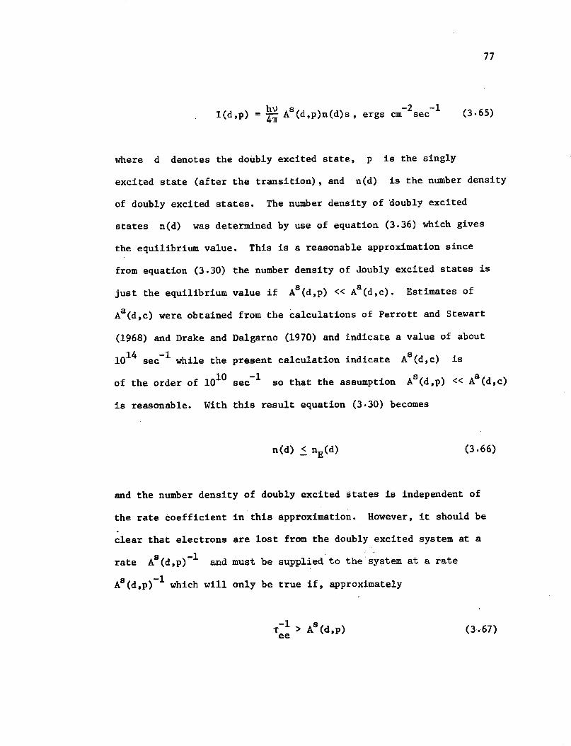
77
I(d,p) = hv A (d,p)n(d)s, ergs cm 2 sec-l (3.65)
where d denotes the doubly excited state, p is the singly
excited state (after the transition), and n(d) is the number density
of doubly excited states. The number density of doubly excited
states n(d) was determined by use of equation (3.36) which gives
the equilibrium value. This is a reasonable approximation since
from equation (3.30) the number density of doubly excited states is
just the equilibrium value if As(d,p) << Aa(d,c). Estimates of
Aa(d,c) were obtained from the calculations of Perrott and Stewart
(1968) and Drake and Dalgarno (1970) and indicate a value of about
1014 sec- 1
while the present calculation indicate AS(d,c) is
of the order of 10 sec- 1
so that the assumption AS(d,p) << A (d,c)
is reasonable. With this result equation (3.30) becomes
n(d) < nE(d) (3.66)
and the number density of doubly excited states is independent of
the rate coefficient in this approximation. However, it should be
clear that electrons are lost from the doubly excited system at a
rate A (d,p)- 1 and must be supplied to the system at a rate
AS(d,p)- 1 which will only be true if, approximately
T-1 > AS(d,p) (3.67)ee
78
-10For the plasma under consideration T e 1 10 sec (Spitzer,
1967) and calculations of AS(d,p), which were discussed in the last
chapter, indicate a value of 1010 sec so that the inequality of
equation (3.67) does not hold completely. Equation (3.36) does,
however, determine an upper limit to the number density of doubly
excited states and, even though the actual density in the experiment
may be well below this value, it is still useful in estimating the
maximum intensity the satellite line would be expected to have.
Since the intensity of the resonance line was determined in coronal
equilibrium rather than LTE, its intensity should be a minimum
[n(q) is coronal equilibrium is less than n(q) in LTE at the same
temperature (i.e. radiation rate > collisional rate)]. Therefore
the ratio of satellite to resonance line intensity should be a
maximum. Under the above conditions the intensity of the satellite
line is
s h4 v nenH ()g(d)A (dA p)sd, -2 -18 3/2 exp kT ergs cm sec (3.68)
(2r mkTe) g(l)
The ratio of equation (3.68) to equation (3.63) is
I h3 g A (d,p) 1 kT=I(L a) (2 mkTe)3/2 2g(l) K(1,2) e
~~~~~~~~~~~~~(-ke
s
(3 .69)
79
where it has been assumed that the frequency of the satellite line
is equal to the frequency of the resonance line to the accuracy
required. Using equation (3.18) for K(1,2) equation (3.69) becomes
3 sR g(d) . As(d,p) E(2,1) expE(2,1)-
(2rmk)3/2 2g(l) 6.5 x 10-
f(l,2)T e )
(3-70)
Setting E(2,1) = ( 4 Z2EH) and writing AS(d,p) in terms of its
oscillator strength [equation (2.67)] the ratio becomes
R = 3.5 x 10⁹ exp (3-71)2k3/2 T f(1,2) ex kT
The oscillator strengths were set equal [i.e., f(d,p) = f(1,2)] since
in both cases the same "inner" electron is "jumping" and this should
be a good approximation. Equation (3.67) was evaluated for each of
the three elements of interest and for temperatures of 50,100,
150,200, and 250 electron volts. These results are given in table
-2, -4III.3 and show that R ranges from 10 to 10 . Values of R
using the expression derived by Gabriel and Paget (1972) (who used
a different excitation cross section including a gaunt factor of 0.2)
are also given in parenthesis. Their ratios are typically a factor
of 2 to 3 higher than those calculated here (for nitrogen). In the
temperature range of interest (Z 200 ev) the satellites would be
extremely difficult to detect and consequently if observed intensity
ratios exceed the calculated values by large amounts the lines could
not be due to transitions from the doubly excited states.
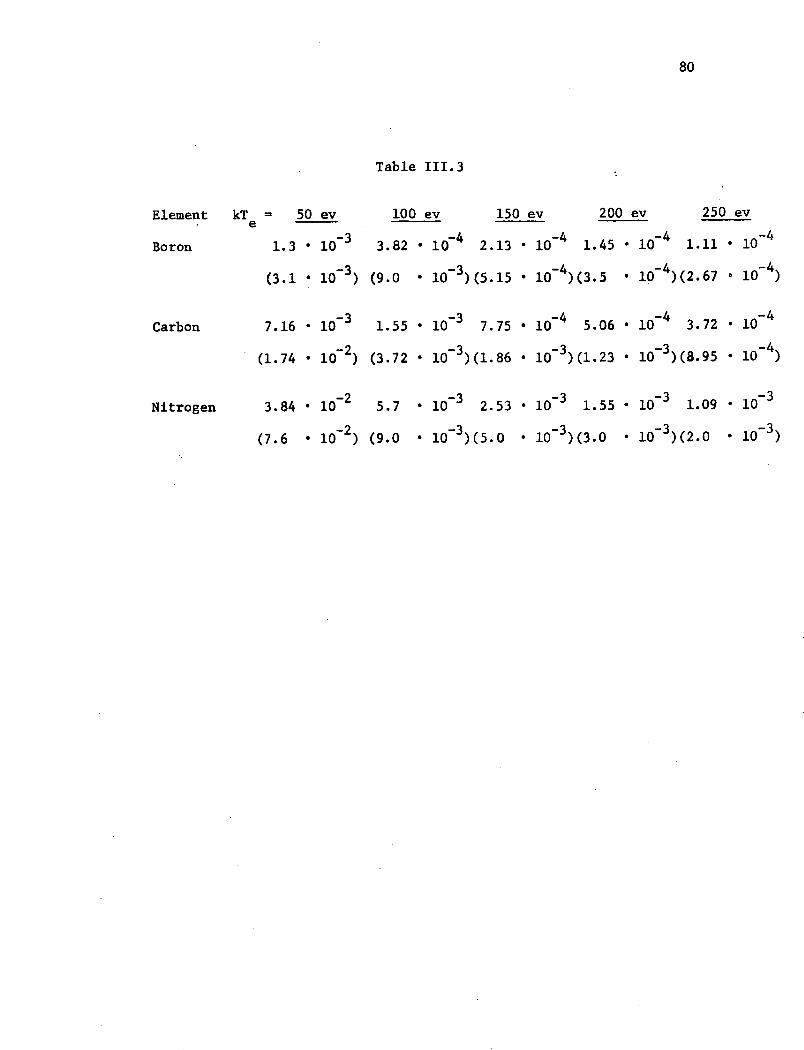
80
Table III.3
Element kT = 50 ev
-3Boron 1.3 * 10
- 3
(3.1 . 10 3)
Carbon
Nitrogen
100 ev 150 ev
-4 -43.82 * 10 2.13 * 10
(9.0 · 10-3 )(5.15 * 1 0- 4
)
7.16 · 10- 3 1.55 * 10
- 37.75 * 10
- 4
(1.74 * 10 -2 ) (3.72 ' 10 3)(1.86 * 10
-3)
3.84 . 10-2 5.7
(7.6 . 10- 2) (9.0
200 ev
1.45 * 10- 4
(3.5 · 10 - 4)
250 ev
1.11 . 10
(2.67 * 10- 4 )
5.06 ' 10-4 3.72 · 10- 4
(1.23 . 10-3)(8.95 . 10- 4 )
10-3 2.53 * 10
-3 1.55 * 10
-3 1.09 · 10
-3
* 10-3)(5.0 · 10-3 )(3.0 * 10 -3)(2.0 * 10- 3 )
CHAPTER IV
EXPERIMENTAL METHOD
A. Theta-Pinch Device
The theta-pinch is one of several devices which were developed
for the production and confinement of high-temperature plasmas
relevant to the study of controlled thermonuclear reactions. The
production of such high-temperature laboratory plasmas at moderate-
to-high particle densities presented the opportunity for the study
of radiation emitted by highly ionized atoms and spectroscopy has
indeed served as a major means of diagnostics on these devices.
Extensive studies in various countries and over a wide range of dis-
charge conditions have established the basic characteristics of
this experimental configuration (Little, et al., 1962; Kolb, et al.,
1962; Goldman, et al., 1962; Beerwald, et al., 1962; and Bodin,
et al., 1962). The theta-pinch utilizes a fast magnetic compression
of an ionized gas to produce the high-temperature plasma. The
rapidly rising magnetic field, which makes the compression possible,
is produced by a large current passing through a single-turn coil
which surrounds the vacuum vessel containing the ionized gas. The
coil and field geometry are shown in Figure 3. The magnetic field
due to the current in the coil may be obtained from the integral
form of Amperes' law (Jackson, 1962)
82PRECEDING PAGE BLANK NOT FILMED
~ · * d = 4z I (4.1)
where I is the total current in the coil in statamps and B is
in Gauss. For the physical arrangement shown in Figure 3 and with
the length k of the coil much greater than its diameter equation
(4.1) gives
B (t) = 7 Ie(t) (4.2)
The time variation in Bz(t) induces an azimuthal electric field
in the ionized gas. This induced current field is given by Faraday's
law
1 aBV x E G at (4.3)
For the particular case of a B field only, equation (4.3) becomes
r a (rEe) 1 i z (4.4)
The applied field has a frequency w and will be attenuated to
l/e of its original value in a distance (Spitzer, 1967; Jackson,
1962)
d = cm. (4.5)
1p - 2 )1
83
where wp is the plasma frequency
CiP
12
-1sec (4. 6)
For a typical experiment, the electron density, ne , is about 1016 cm-3
which gives
Wp = 5.6 x 10¹²
Typically, the driving field frequency w
105 sec -1 , so that
. << 1
The depth of penetration is then
is of the order of
d = c = 0.536 x 10⁻² cm
WI,
and the fields are restricted to
The radial electric field, Er,
to symmetry of the coil so that
becomes
the surface of the plasma cylinder.
should be independent of 8 due
aE ra8 may be ignored. Equation (4.4)
aBE = r z
E8 2c at (4.7)
-1sec
84
with Bz equal to its value at the surface of the plasma and r
equal to the radius of the plasma column.
The induced current then follows from Ohm's law
J = aE
where a is the conductivity of the plasma. The induced current
density is then
3B
JiB = Ee = 2 (4.3)
The Lorentz force acting on the plasma surface inward is given by
F= Jie x B (49)r c ie z
The current sheet initially moves inward at a high velocity and
heats the plasma. Further compression of the plasma occurs
adiabatically when the thermal energy of the plasma particle exceeds
the velocity of the current sheet. If end losses and radiation
cooling are ignored, the plasma will be compressed until the magnetic
pressure is equal to the internal pressure
= nkT + nkT (4.10)8Tr =e ei
85
The sum must extend over all of the various ions at their individual
temperatures. In general, the electrons and the ions will be at
different temperatures, since the electrons are compressed adia-
batically during compression of the plasma while the ions are shock
heated (Rose and Clark, 1961). In fact, the average radial speed
of the current sheet is of the order of 107 cm/sec. For the electrons
this velocity corresponds to a mean thermal energy of about 0.04 eV
which is considerably less than their actual energy which will be of
the order of a few eV, thus adiabatic compression results. For ions
the situation is quite different. The velocity of 107 cm/sec
corresponds to a mean thermal energy of 150 eV for deuterons and the
initial velocity of the deuterons will be much less than this. Since
the mean thermal velocity of the ions is less than the velocity of
the current sheet a shock wave will develop and the ions will be
heated by the passage of the shock wave (Rose and Clark, 1961).
However, since collisional rates for electrons exceed those for ions
it is the electron temperature that is generally of interest in the
discussion of the various atomic processes.
A common feature of the magnetically compressed plasma experi-
ments is the existence of a trapped internal magnetic field which,
depending on the plasma conductivity and breakdown conditions, can
reach large values antiparallel to the external field during compres-
sion. A number of authors (Kolb, 1959; Fay, Hintz, and Jordan, 1959;
Kolb, Dobbie, and Griem, 1959) have observed that the strength, sign,
and spatial distribution of the initially trapped magnetic field are
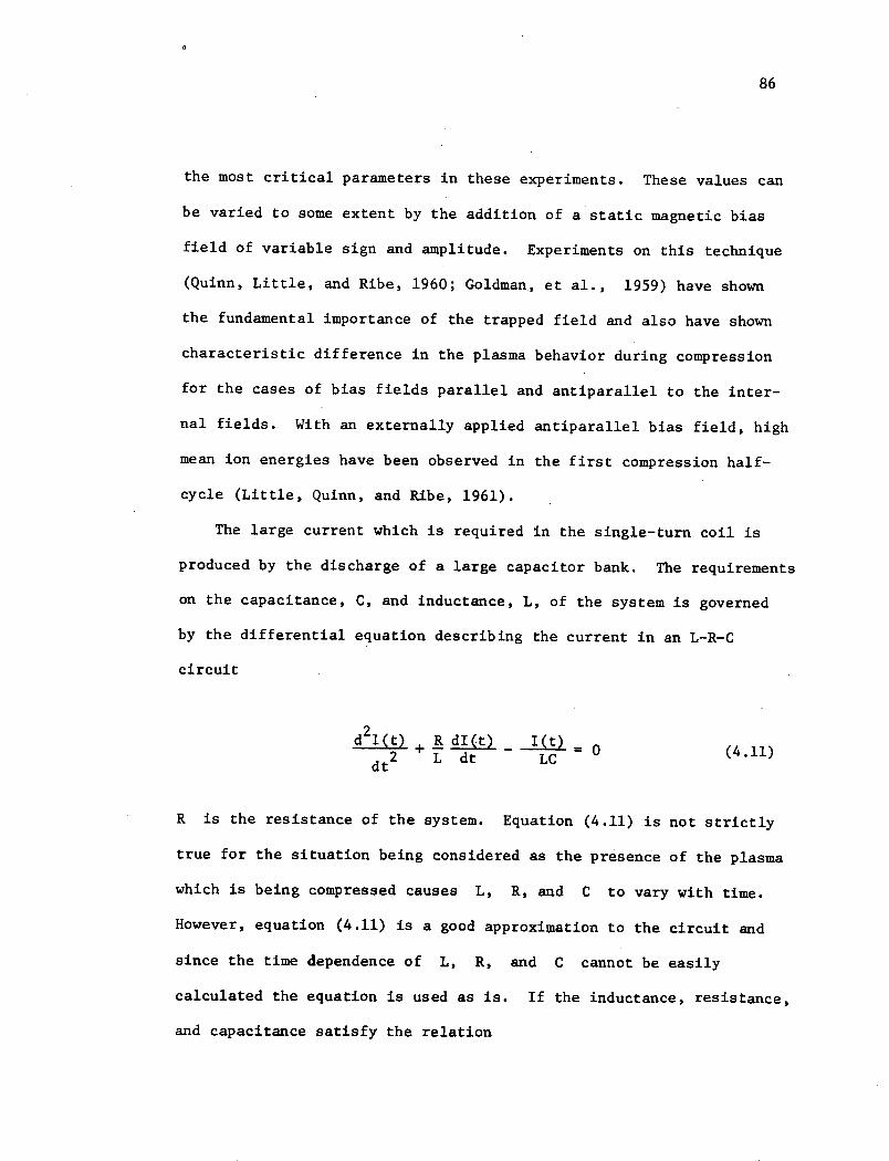
86
the most critical parameters in these experiments. These values can
be varied to some extent by the addition of a static magnetic bias
field of variable sign and amplitude. Experiments on this technique
(Quinn, Little, and Ribe, 1960; Goldman, et al., 1959) have shown
the fundamental importance of the trapped field and also have shown
characteristic difference in the plasma behavior during compression
for the cases of bias fields parallel and antiparallel to the inter-
nal fields. With an externally applied antiparallel bias field, high
mean ion energies have been observed in the first compression half-
cycle (Little, Quinn, and Ribe, 1961).
The large current which is required in the single-turn coil is
produced by the discharge of a large capacitor bank. The requirements
on the capacitance, C, and inductance, L, of the system is governed
by the differential equation describing the current in an L-R-C
circuit
d2I(t) + R dI(t) I(t) (4.11)dt2 L dt LC
R is the resistance of the system. Equation (4.11) is not strictly
true for the situation being considered as the presence of the plasma
which is being compressed causes L, R, and C to vary with time.
However, equation (4.11) is a good approximation to the circuit and
since the time dependence of L, R, and C cannot be easily
calculated the equation is used as is. If the inductance, resistance,
and capacitance satisfy the relation
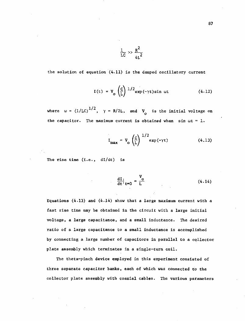
87
1 >> R2
LC 4L2
the solution of equation (4.11) is the damped oscillatory current
I(t) = V () / 2exp(-yt)sin wt (4.12)
1/2where w = (1/LC) , y = R/2L, and V is the initial voltage on
the capacitor. The maximum current is obtained when sin wt = 1.
/ 1/2Imax = V0 (L) exp(-yt) (4.13)
The rise time (i.e., dI/dt) is
V
dtiLtt=O 0L (4.14)
Equations (4.13) and (4.14) show that a large maximum current with a
fast rise time may be obtained in the circuit with a large initial
voltage, a large capacitance, and a small inductance. The desired
ratio of a large capacitance to a small inductance is accomplished
by connecting a large number of capacitors in parallel to a collector
plate assembly which terminates in a single-turn coil.
The theta-pinch device employed in this experiment consisted of
three separate capacitor banks, each of which was connected to the
collector plate assembly with coaxial cables. The various parameters
88
of these banks are listed in table IV.1. The bias field bank
established the slowly varying reverse magnetic field, while the
preheater bank heated and ionized the cold gas in the shock tube.
The large current required to produce the high magnetic field which
compresses the ionized gas was obtained by the discharge of the main
capacitor bank. This bank consisted of 410 capacitors connected in
parallel with one triggered spark gap for each pair of capacitors.
The bank could be switched in less than 25 nanoseconds (Oertel and
Williams, 1965). The single-turn coil had an inside diameter of 10
centimeters and was constructed of nine segments , each of which was
15 centimeters long. The segments were assembled with a 0.25 cm gap
between segments so that observations could be made perpendicular
to the longitudinal axis of the coil. This arrangement gave a
total coil length of 137 cm. The shock tube was constructed of
quartz (SiO2) and had an outside diameter of 9.6 cm., a wall thickness
of 0.5 cm., and a total length of 183 cm. The general physical
arrangement of the experiment is shown in Figure 4 and a schematic
of the electrical circuit is shown in Figure 5.
A schematic of the vacuum system is shown in Figure 6 and con-
sists of a mechanical pump which may be used to evacuate the entire
system to about 10- 2 torr and a turbomolecular pump which evacuates
the system to pressures of about 10-9 torr. The turbomolecular pump
is basically a turbine type and its principle of operation is a gas
molecule-wall collision process. The molecules enter the pump at the
inlet port, collide with all of the interior surfaces of the inlet
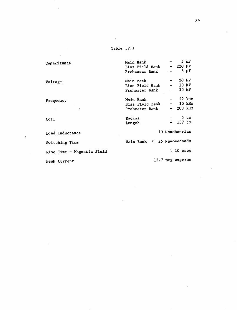
89
Table IV.1
Main BankBias FieldPreheater B
Main BankBias FieldPreheater B
Main BankBias FieldPreheater B
RadiusLength
Frequency
Coil
Load Inductance
Switching Time
Rise Time - Magnetic Field
Peak Current
Main Bank
- 5mF
Bank - 220 pF;ank - 5 pF
- 20 kV
Bank - 10 kV3ank - 20 kV
- 22 kHz
Bank - 10 kHz
lank - 200 kHz
- 5 cm- 137 cm
10 Nanohenries
< 25 Nanoseconds
z 10 psec
12.7 meg Amperes
Capacitance
Voltage
90
portion and some of them are accelerated axially toward the ends of
the pump when they are struck by the blades on the first rotating disk
(rotating at 16,000 RPM). The molecules are guided in the proper
direction by impinging upon the first set of fixed blades which are
oriented in such a fashion as to increase the probability of the
molecules being struck by the second set of rotating blades. This
process is repeated through several stages (nineteen on each side for
the particular pump used) resulting in a compression of the gas. This
compression depends on the relative motion of the blades and molecules
with the compression increasing as the blades move faster relative
to the molecules. The compressed gases are removed by the mechanical
pump and exhausted to the atmosphere. The leak rate of the vacuum
system was investigated by evacuating the system to its lowest pressure
and then closing the valve between the vacuum pump and the shock
tube. The pressure in the system was measured by means of a nude
ion gage and it was found that the system pressure had reached
1 x 10 torr at the time the fill gas was admitted into the shock
tube. While this leak rate was rather high it was thought at the
time that the background particle density at 10 6 torr (z 3.5 x 101
cm ) would not interfere critically with the investigation since
most experiments of this type employ oil diffusion pumps to evacuate
their systems and normally work with a base pressure of this magnitude.
Furthermore, the leakage was thought to be past the viton "0" rings
which sealed the quartz tube to the vacuum system and to repair
the leak would have required considerable time and effort. The leak
91
was located in the latter part of the experiment and was actually
due to leakage past a valve stem which was repaired by simply re-
placing the valve. The operating conditions for the experiment are
listed in table IV.2.
The various elements whose spectra were to be investigated were
introduced into the deuterium fill gas prior to its introduction into
the shock tube. To insure that the gases were well mixed, a stain-
less steel tank equipped with a slowly rotating paddle was connected
directly to the vacuum system and served as a mixing and storage
tank. This tank was filled with deuterium to a predetermined pressure,
and the amount of the specific element required was added in a
gaseous form to obtain the desired percentage of the element in the
mixture. Carbon spectra were obtained by the introduction of methane
(CH4) or acetylene (C2H2), boron spectra by the introduction of di-
borane (B2H6), and nitrogen spectra by the introduction of molecular
nitrogen (N2). Normally, a volume sufficient for several hundred
shock tube fillings was mixed at one time, insuring that the gas
mixture did not change during the course of the investigation. The
amount of the impurity element which could be added was restricted
to 5 percent of the total volume. At higher concentrations, the
plasma did not reach a sufficiently high temperature due to radiation
losses, or the plasma column became subject to violent instabilities.
The gas was introduced into the shock tube through a leak valve.
The pressure in the shock tube was continuously monitored during
filling by means of a calibrated thermocouple gage. A filling
pressure of 50 millitorr, corresponding to a particle density of
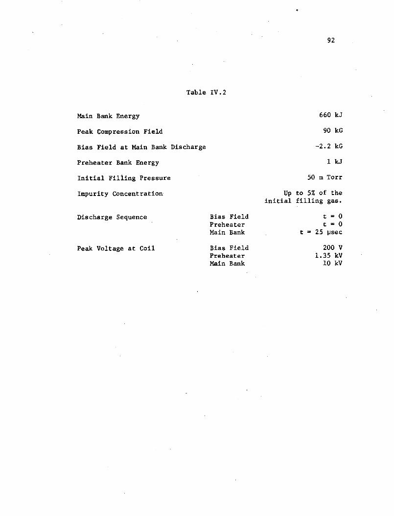
92
Table IV.2
Main Bank Energy
Peak Compression Field
Bias Field at Main Bank Discharge
Preheater Bank Energy
Initial Filling Pressure
Impurity Concentration
Discharge Sequence
Peak Voltage at Coil
Bias FieldPreheaterMain Bank
Bias FieldPreheaterMain Bank
660 kJ
90 kG
-2.2 kG
1 kJ
50 m Torr
Up to 5% of theinitial filling gas.
t=0t=0
t = 25 psec
200 V1.35 kV
10 kV
93
15 -31.8 x 10 cm , was used in this experiment, as it was experi-
mentally determined that a higher filling pressure produced a plasma
of insufficient temperature while a lower filling pressure did not
produce spectral lines of sufficient intensity to allow photographic
recording with a single discharge. After filling the shock tube,
the three capacitor banks were charged and then dicharged in a
predetermined sequence. The bias field bank and the preheater bank
were discharged at the same time, producing a voltage at the coil
which consisted of the slowly varying voltage from the bias field
bank with the higher frequency voltage from the preheater bank
superimposed. The time at which the main bank was discharged was
determined by the requirement that the preheater plasma be relatively
stable and have a high degree of ionization at the start of the
magnetic compression phase. An investigation of the preheater plasma
indicated that a stable plasma having an electron density of about
1015 cm-3 and an electron temperature of from 1 to 2 electron volts
existed at 25 microseconds after the preheater bank had been
triggered (Oertel and Jalufka, 1966). This time delay for the dis-
charge of the main bank was used throughout this investigation.
An image converter camera, operated in the streak mode, was
employed to investigate the compression of the ionized gas. The
camera viewed a 0.25 cm portion of the plasma column through the
slit between two of the coil sections and near the center of the coil
assembly. The image of the plasma portion was streaked across a
film by the camera and the resulting photograph showed the time
history of the plasma column diameter during the Fompression of the
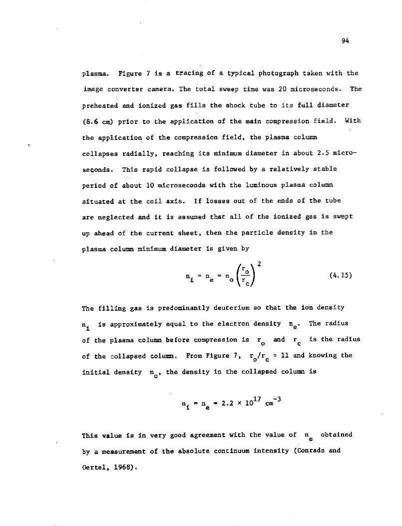
94
plasma. Figure 7 is a tracing of a typical photograph taken with the
image converter camera. The total sweep time was 20 microseconds. The
preheated and ionized gas fills the shock tube to its full diameter
(8.6 cm) prior to the application of the main compression field. With
the application of the compression field, the plasma column
collapses radially, reaching its minimum diameter in about 2.5 micro-
seconds. This rapid collapse is followed by a relatively stable
period of about 10 microseconds with the luminous plasma column
situated at the coil axis. If losses out of the ends of the tube
are neglected and it is assumed that all of the ionized gas is swept
up ahead of the current sheet, then-the particle density in the
plasma column minimum diameter is given by
ni n no (4.15)ni ne o
The filling gas is predominantly deuterium so that the ion density
ni is approximately equal to the electron density ne. The radius
of the plasma column before compression is ro and rc is the radius
of the collapsed column. From Figure 7, ro/r 11 and knowing the
initial density no, the density in the collapsed column is
ni = ne = 2.2 x 1017 cm-3
This value is in very good agreement with the value of ne obtained
by a measurement of the absolute continuum intensity (Conrads and
Oertel, 1968).
95
The electron temperature of the plasma was determined by the line
intensity ratio method assuming corona equilibrium which was justi-
fied in Chapter III. The intensity of a spectral line is given by
equation (3.47) and the ratio R of the intensities of two spectral
lines corresponding to transitions between states p, q in an ion of
charge Z + 1 and states i, j in an ion of charge Z is
R I(p,q,Z + 1) _ NZ + l(q)A(p,q)A(i,j) (4.16)I(i, J, Z) NZ(j)A(i,j) X(p,q)
The density ratio of the upper states of the lines may be obtained
by assuming that the states are populated by electron collisions from
the ground state only as in the coronal approximation and ignoring
effects due to cascading. Using the expression due to Seaton (1962)
for the threshold excitation of ions, the ratio of the upper states is
Nl'(Z+lq) NZ+(1) f(r,q)E(s,j) expE( - E(1q)(417)Z exp kTe (4.17)
N (j) N (l)f(s,j)E(r,q) e
where N Z+(1) and NZ(1) are the ground state population, the f's
are the absorption oscillator strengths, and the E's are the exci-
tation energy of the excited states above the ground states. The
ground state density ratio is obtained from the corona equilibrium
ionization equation. Using the expression given by McWhirter (1965),
which ignores dielectronics recombination
96
z+1 1 kT 3/4= 1.27 x 10 / exp k
e
(4.18)Z Z kT
N (1) E e
EZ is the ionization potential of the species of charge Z. Time
dependency has been ignored in equation (4.18) since the data was
obtained in a time integrated mode so that only average values were
obtained. This dependency would have to be considered if time
resolved intensities were recorded as there is some indication that
lines of a given stage of ionization appear at a higher temperature
in transient plasmas with rapidly rising temperature than in the
steady state coronal approximation. This is due to the finite
relaxation times of the ionization processes (Kunze, Gabriel,and
Griem, 1968). Equation (4.18) may therefore indicate a lower
temperature than that actually obtained. The effect of ignoring
dielectronic recombination may be estimated from the ionization
balance calculations for oxygen including radiative and dielectronic
recombination (Burgess and Summers, 1969). A comparison of their
values with those calculated from equation (4.18) indicates that at
16 -3electron densities of 10 cm , the effect of including dielectronic
recombination is to shift the curves to a higher temperatures (by
about. 20%). At the higher densities obtained in this experiment
(i.e., 2.2 x 10 17cm -3 ) the effect should be less due to the inverse
dependence of the dielectronic rate coefficient on the electron
density. At lower electron densities the effect would increase up to
a discrepency of a factor of 2 in the solar corona (ne ~ 108 cm3).
97
McWhirter indicates that equation (4.18) should be accurate to + 50%
for the ratio of hydrogen-like ions to bare nuclei (no dielectronic
recombination possible for this case) but also points out that the
strong influence of the exponential should allow temperature to be
estimated to an accuracy of 10%. For the ratio of helium-like to
hydrogen-ions the results should be considerably poorer and the
above discussion would indicate that a factor of up to two in
temperature may be obtained. Substituting equations (4.17) and (4.18)
in equation (4.16), the intensity ratio becomes
R= A(p,q)X(i,j)f(l,q)E(1,j)l.27 x 10( 3/4e exp ( -E( >
A(i,j)X(p,q)f(l,j)E(l,q)( Z) 2 Te
(4.19)
If the resonance lines of the two successive stages of ionization
are used, then p = 1 and i = 1 . Equation (4.19) was evaluted
for the resonance lines of the hydrogen-like and helium-like ions of
oxygen over the range of temperatures expected. The results are
plotted in Figure 8 and the graph was then used to determine the
plasma electron temperature. Including the effects of dielectronic
recombination would shift the curve to about a 20% higher temperature.
Oxygen was chosen as the most convenient element since it is in-
jected into the plasma from the shock tube walls during the preheating
phase and also because the two resonance lines were separated by
0 0 oonly 2.63 A, (i.e., 21.602 A for helium-like and 18.969 A for
hydrogen-like) so the problem of film response as a function of
98
wavelength was virtually eliminated. The intensities of the two
lines were measured from the microdensitometer trace of the spectra
which had been recorded on film. The spectra were recorded in the
time-integrated mode and the resultant intensities represented an
average over several cycles of plasma compression and expansion so
that the temperature obtained was at best an estimate. Furthermore,
the approximation that the upper states of the lines were populated
from the ground state only is somewhat suspect since both ions have
meta-stable states lying below the upper state of the resonance line.
These meta-stable states can be populated by radiative transitions
from higher states and, since they cannot decay to a lower state,
are depopulated by electron collisions. Thus the upper states of the
resonance lines may also be populated by electron collisions from
the meta-stable states. (Gabriel and Jordan, 1969) However, the
electron temperature obtained in this manner varied from 160 eV to
220 eV, which is in good agreement with the measured temperature
reported in other similar devices (Roth and Elton, 1968; Sawyer,
et al., 1962). More accurate measurements of the electron temperature
carried out on a similar experiment and based on Thompson scattering
of laser light indicate higher temperatures, up to about 240 eV.
(Kunze, Gabriel and Griem, 1968). This latter result appears to be
more in agreement with the inclusion of dielectronic recombination.
However the higher temperature would decrease the intensity ratio of
satellite to resonance line due to the T 1 dependence. At the lower
temperatures (i.e., T < 200 eV) the calculations of Landini and
Fossi (1971) indicate that dielectronic recombination should be
99
important but not dominant. Using a simple result of Goldberg (1966)
the temperature at which dielectronic recombination is expected to
be a maximum is just equal to the wavenumber of the recombining ion
so that the lower temperature should be appropriate for boron V while
the higher temperatures would be more compatable with carbon VI.
The relevant plasma parameters are listed in table IV.3.
B. Grazing Incidence Spectrograph
The hydrogen-like resonance lines of the elements investigated
0all lie below 50 A,which is beyond the range of normal incidence
vacuum spectrographs. The spectra were therefore obtained at grazing
incidence with a 1-meter radius of curvature, platinum-coated grating
rules with 3,600 lines/millimeter (Leybold-Heraeus GMBH and Co.).
The theory of the concaved grating and its use in the grazing
incidence mounting has been discussed in detail (Samson, 1967;
Beutler, 1945; Namioka, 1959, 1961; Mack, Stehn, and Edlen, 1932)
and no useful purpose would be served by repeating these discussions
here. Therefore, only those parameters of the grating and the
grazing incidence mounting which are pertinent to the analysis of
laboratory spectra will be discussed.
The optical arrangement for the grazing incidence mounting is
shown in Figure 9. The concave grating of radius of curvature R
is mounted tangent to the Rowland circle of radius R/2. If the
entrance slit lies on this circle at an angle of incidence a,
then the image will lie on the circle at an angle of diffraction 3.
These two angles are related by the grating equation
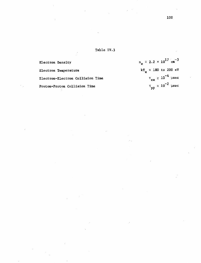
100
Table IV.3
Electron Density
Electron Temperature
Electron-Electron Collision Time
Proton-Proton Collision Time
n = 2.2 x 1017 cm 3
kT z 180 to 200 eV
T z 10-4 psecee
T z=10-2
IsecPP
101
mA = a(sin a + sin B) (4.20)
The grating factor a is the reciprocal of the number of lines pero
Angstrom ruled on the grating, m is the order of the spectrum, and
X is the wavelength of the spectral line in Angstroms. The disper-
sion of the grating expresses how the various wavelengths are distri-
buted along the Rowland circle. The angular dispersion d$/dX is
obtained by differentiating equation (4.20). For a fixed angle of
incidence (a = constant)
dS mdA a cos 8 * (4.21)d-'
=
a cos a
For an analysis of the spectrum, the actual number of angstroms
per millimeter dispersed along the Rowland circle is of more interest.
This quantity is called the plate factor and is the reciprocal of
the linear dispersion. The plate factor may be obtained from equation
(4.21). Referring to Figure 9
dX = dA do (4.22)da dB di
and
d =- - RdB (4.23)
102
With these substitutions, equation (4.21) becomes
dA a cos 6(424)d4 mR
In the grazing incidence mounting, the dispersion changes rapidly
with increasing wavelength so that the linear relationship used for
normal incidence mountings is not applicable and the dispersion curve
must be determined if accurate wavelength measurements are to be
made. Figure 10 is the theoretical dispersion curve which was cal-
culated for an 85° angle of incidence and a 1-meter radius of curva-
ture grating ruled with 3,600 lines per millimeter corresponding to
the instrument used in the experiment.
Closely related to the dispersion is a quantity known as the
resolving power. While the dispersion determines the separation of
two wavelengths (spectral lines), the resolving power determines
whether this separation can be distinguished. Each monochromatic
beam from the grating forms a diffraction pattern, the principal
maxima of which are represented by the order number m. Between
these principal maxima, secondary maxima are formed whose intensities
decrease as the number of ruled lines N exposed to the incident
radiation increase. In a normal laboratory instrument, these
secondary maxima are very much weaker than the principal maxima.
The angular half-width of a principle maximum dB is the angular
distance between the principal maximum and its first minimum and, for
a plane grating, is given by the expression
103
d= No (4.25)
This width provides a theoretical limit to the resolving power of
the grating. If Rayleigh's criterion is used, two lines of equal
intensity will just be resolved when the maximum of one falls on the
minimum of the other. The resolving power P is defined as X/dA,
where dX is the minimum wavelength separation which can be resolved.
This minimum wavelength separation may be expressed in terms of d8
dld d = d (4.26)
Substituting in equation (4.25) the resolving power is obtained
P d = mN (4.27)
Equation (4.27) represents the theoretical limit of the resolving
power and whether this limit is achieved will depend on the quality
of the grating. The finite width of the entrance slit is also a
major factor in determining the resolution of a given instrument.
For the concave grating mountings the entrance slit to grating dis-
tance is equal to the image to grating distance so that the image
width can be no less than the slit width. This width, and hence
a measure of the limit of resolution imposed by the slit, may be
obtained by multiplying the slit width in millimeter by the equation
104
0(4.24) in A/mm. This value of dA ( and X at which it is
calculated) may then be used to obtain the resolution limit [equation
(4.27)]due to the slit width. It is clear from equation (4.27)
that the resolving power increases with the order number, m. The
major aberration of the concave diffraction grating is astigmatism,
which results in a point on the vertical entrance slit being imaged
into a vertical line; that is, focusing is achieved only in the
horizontal plane. (i.e., perpendicular to the slit height) The
theory of the astigmatism of a concave grating was first developed
by Runge and Munnkopf (1927). More recently the problem has been
dealt with in detail by Beutler (1945) and Namioka (1959, 1961). The
length of the astigmatic image is given by (Beutler, 1945)
[ cos s] + L[sin a tan a cos ] (4.28)
where the first term gives the contribution due to the entrance slit
of finite vertical length Z and the second term is the astigmatism
produced by a point on the entrance slit. L represents the length
of the ruled lines illuminated. Equation (4.28) indicates that the
image becomes less astigmatic near normal incidence and that astig-
matism is most severe at grazing incidence. While this astigmatism
does not cause the spectral line to be less sharp in the grazing
incidence mount it does greatly reduce the energy per unit length
received at the focal plane. For the grating used in this experiment
and with a 850 and 800 (corresponding to X 30 A) theand with a = 85° and B = 80° (corresponding to X = 30 A) the
105
first term of equation (4.28) contributes approximately 2Z to the
height while the second term contributes about 3L to height.
While some control may be exercised over the first term it is normally
small relative to the second term which for a given instrument is
controlled by the height L of commercially available grating. It
is possible,-of course,to mask the grating and reduce L but the
improvement in the image height is gained at the expense of
reduced intensity per unit area at the focal plane, since both inten-
sity and astigmatism are proportional to L.
Equation (4.27) is strictly true for a plane grating but is also
applicable to a concaved grating if the width of the grating is less
than its optimum value which is given below. Namioka (1959, 1961)
and Mack, Stehn, and Edlen (1932) have shown that for a concave grat-
ing the angular half-width of the principal maximum deviates from
that given by equation (4.25) and that the diffracted minima do not
reach zero. Therefore, a modified Rayleigh criterion was intro-
duced which states that two lines of equal intensity will be just
resolved when the wavelength difference between them is such that
the minimum total intensity between the lines is 8/r 2 (= 0.8106)
times as great as the total intensity at the central maximum of
either of the lines. With this new criterion, they have shown that
the resolving power of a concave grating is equal to mN when the
width W of the grating illuminated is less than or equal to Wopt
1.18. The optimum width is obtained from physical optics (Samson,
1967),
106
W = 2.51 R3A cos a cos B /4
sin2a cos B + sin2 cos a /
For the 1-meter radius of curvature grating used in this experi-
ment at an angle of incidence of 850, the optimum width for a
detected wavelength of 50 A is 3.34 millimeters, which is much
smaller than the actual width of the 20-millimeter-wide grating used.
The greater width of the grating is beneficial in increasing the
intensity of a line in the focal plane, since intensity is propor-
tional to the area of the grating illuminated. Since the investiga-
tion required the recording of spectra from a pulsed discharge of
very short duration and since it was desired to record spectra with a
single discharge some resolution had to be sacrificed in order to
obtain sufficient intensities at the focal plane (i.e., a larger
grating was used in order to get more intensity which is dependent
on the ruled area of the grating). Thus the grating employed was a
compromise which gave adequate resolution with sufficient intensity.
For gratings having widths greater than the optimum width the
resolution is given by (Samson, 1967)
P - 0.75 (Wt) m (4-30)
Thus, if W > Wopt the resolution is independent of the width.opt
Solving equation (4.30) for the grating used in the experiment,
the theoretical resolving power of the grating is
107
X z 104 (4.31)dX
The actual resolution of the instrument does not depend on the
grating alone but depends on the slit width also. The slit must be
narrow enough to provide adequate resolution but still of sufficient
width to allow an adequate amount of light to pass.(i.e., the wider
the slit the more light is passed through.) Mack, Stehn, and Edlen
(1932) treat the slit and grating together, which is necessary if
the resolving power of each of the two elements is nearly equal.
If the resolving power of one element is greatly different from the
resolving power of the other element, then the resolving power of
the combination is determined by the smaller value. In practice
this is generally the case, with the resolving power being determined
by the slit width. The resolution is also degraded by thermal
broadening of spectral lines in the light source and also by the
film. For these reasons, it is more convenient to establish the
instrument resolution experimentally. This was accomplished by
recording, on film, the spectrum of a high-temperature aluminum
plasma, produced by firing a large pulsed ruby laser at a solid
aluminum sample. A microdensitometer trace of the film showed the
.0aluminum VIII lines at 66.704 A and 66.731 X to be clearly resolved.
Therefore, the resolving power at 66 A is
Tx > 2000 (4.32)d'" 20
108
This procedure was also used to establish the optimum slit width.
A series of exposures taken of the plasma with various slit widths
showed that a slit width less than 17 microns only decreased the
intensity of the spectral line of the film without improving the
resolution. The calculated value of P corresponding to this
width and at a wavelength 66.7 A is P- 6,000. This slit width was
used for all spectra recorded in this experiment.
The physical arrangement of the components is shown in Figure 11.
The adjustable entrance slit, grating, and film holder are mounted
on a base plate with the grating holder and film holder attached to
arms pivoting around the center of the Rowland circle. The base
plate is mounted so that it may pivot around a vertical axis through
the center of the entrance slit. This arrangement allows the angle
of incidence to be varied between 800 and 890 without movement of the
vacuum housing or the experimental arrangement.
An aperture was inserted in the vacuum system between the shock
tube and the entrance slit of the spectrograph. This aperture con-
sisted of a 5-millimeter-diameter circular hole in a copper disk
about 1 millimeter thick. The disk was clamped between two flanges
with the geometrical center of the circular hole on the optical axis
of the system. This aperture prevented the spectragraph from "seeing"
the walls of the shock tube and, consequently, the radiation emitted
by the surface of the tube.
Photographic recording of spectra allows the recording of all
wavelength and line intensity data in a rather large portion of the
109
spectrum with a single (or multiple) discharge of a laboratory experi-
ment. This is a distinct advantage if the plasma produced by the
experiment is not sufficiently reproduceable which is often the case.
The determination of intensities from the developed photographic
film, however, cannot be done directly. The quantity which can be
measured directly from the film is the photographic density D which
is related to the transmission T of the film. For visible and
ultraviolet light this relationship is (Mees, 1963)
D - Log1 0 (1/T) (4.33)
This photographic density is produced by the exposure E which is
the energy received by a square centimeter on the photographic layer
during the exposure time te. If the light flux is denoted by F(t)
the exposure is
i= j F(t)dt (4.34)0
The density D which is produced on the film will depend on other
factors such as development time and temperature, the developer
solution used, age of the film and wavelength of the exposing light.
The quantities T and D cannot be absolutely defined as their
measurement willdepend on the densitometer used (light sources,
transmission of various components etc.). Therefore the film is
normally calibrated by exposing a section to a standard light source
110
with different exposures. This is normally done by the use of a
stepped filter having transmissions of 100% to about 1%. The film
is then developed in the normal way and the density for each exposure
measured. The characteristic curve (H-D or Hurter-Driffield curve)
is then constructed by plotting the density D versus log1 0 i. A
typical curve experimentally obtained in this manner is shown in
0Figure 12. In the wavelength region below about 100 A the above
relationships do not hold. The large photon energies in this region
are sufficient to make an emulsion grain developable by the absorp-
tion of a single photon compared to the 3 or 4 required per grain in
the visible region. Thus if the film density D is plotted versus
the exposure i a straight line is obtained (Mees, 1963). This
situation eliminates the threshold of the emulsion which is commonly
encountered with the lower energy photons. A typical characteristic
curve obtained experimentally for this short wavelength radiation is
shown in Figure 13. Obtaining the necessary characteristic curve for
an emulsion in this region is extremely difficult due to a lack of
standard sources and density filters for use in the region. Since
relative line intensities were needed in order to determine the
electron temperature the following procedure was carried out in
order to obtain some information about the film characteristics.
Two different film strips (from the same roll) were employed, the
first being exposed to a single discharge and the second to two
discharges. In each case the initial filling pressure, bank voltage
and all other controllable parameters were the same. Furthermore
111
monitoring of the continuum intensity (proportional to the electron
density) and the temperature insure that these parameters were the
same within a few percent on each discharge. The films were then
developed in the same solution for the same length of time and then
dried. These two films were then scanned on a microdensitometer at
the same sensitivity. Spectral lines throughout the region of
interest were compared and in each case their peak intensities
differed by 'about a factor of two indicating that the film response
was approximately linear in the region if zero threshold is assumed.
One disadvantage of the instrument is that the small diameter
of the Rowland circle (100 cm) prevents the standard thickness of
SWR glass plates from being used, as it proved impossible to bend
them to the required curvature without breakage. This particular
difficulty could be overcome to a certain extent by the use of
Ilford Q-2 plates. However, the emulsion on the Q-2 plates
saturated at a rather low level so that in order to record weak lines
it was necessary to grossly overexpose the more intense lines. The
data were finally recorded on 35-mm Eastman Kodak SWR film. This
film was not completely satisfactory, as it has a tendency to
stretch somewhat during development. The film also initially pre-
sented a problem in keeping it on the Rowland circle, as it tended
to curve after having been clamped in place and placed under vacuum.
This problem was resolved by mounting the film strip between two
flat, thin metal strips in a sandwich arrangement. The outer strip
had a horizontal slot 1 cm wide to allow the radiation to strike the
film. Further improvement was obtained by clamping only one end of
112
the film in the holder and then evacuating the system. The clamping
arrangement could be controlled from outside the vacuum so that the
second end of the film could be clamped after the required vacuum
was obtained. Some further disadvantages were encountered with the
films that also occur with the glass plates. This is the normal
difficulty with the Schumann-type emulsions which consist of grains
of emulsion supported from behind by a thin layer of gelatin. These
emulsions are very sensitive to pressure fogging, scratching, and
dust, which requires that they be handled with the utmost care. There
is also some variation in the sensitivity of the emulsion from box
to box.
After a film had been placed in the instrument and the instrument
had been evacuated, the recording of a spectrum proceeded in the
following manner. A valve between the spectrograph and the shock
tube was kept closed while the shock tube was evacuated to its base
pressure and then filled with gas. The capacitor banks were then
charged and, with the valve still closed, the discharge was initiated.
This procedure was followed and carried out a minimum of five times
before the valve between discharge and spectrograph was opened and
the exposure made. This procedure "cleaned up" the shock tube as
the accumulate contamination on the walls of the shock tube were
burned off by these preliminary discharges. Normally, a good exposure
was obtained with a single discharge.
After a film had been exposed, it was removed from the instrument
and developed. These films were developed by constant agitation for
113
4 minutes in Kodak D-19 developer diluted in the ratio of three
parts water to one part developer. The.film was then rinsed in
deionized water for 10 seconds and then immersed in Kodak Rapid Fix
for 4 minutes. The fixing was followed by a 12-minute wash in
running water and then dried at room temperature (23° C). The temp-
erature of the developer, rinse, and fixer was kept at room tempera-
ture and the same development procedure was followed on each film.
After the film had dried, it was examined visibly and the necessary
identification information was put on the film. The film was then
scanned on a microdensitometer and the film, along with the tracings,
was stored until ready for data analysis.
In order to insure that the plasma conditions did not vary
excessively from discharge to discharge, a monitor system consisting
of a 1-meter focal length, normal incidence vacuum monochromater
(McPherson Instrument Corp.) using an EMI 6256 photomultiplier tube,
and a 1-meter focal length Czerny-Turner monochromater (McPherson
Instrument Corp.) using an Amperex 150 AVP tube was employed. The
vacuum instrument measured the total intensity of the ls2s S1 -
330 o0 33ols2p 3 P transition at 1637.96 A and the ls2s 3S
1- ls2p 3P0 at
1639.58 A of 0 VIII together. In order to obtain the high stage of
ionization from which this radiation is produced, a fairly high
temperature is required. By recording the intensity of the line on
an oscilloscope, a time history was obtained. The appearance of this
line with a reasonable intensity was sufficient to indicate that
compression of the plasma had taken place and in conjunction with the
114
second monochromater signal, which was indicative of the density,
indicated that the electron temperature had reached an acceptable
0value. The second monochromater measured the intensity in a 15 A
owide band at 5221 A . At the high temperatures obtained in the plasma,
the radiation at this wavelength should be due to bremsstrahlung.
This was verified by spectra of the plasma recorded in this region
which showed no line radiation other than that from low stages of
ionization which would not exist at the higher temperature. The
particular region used showed no line radiation at all, so the
recorded signal was due to continuum radiation. Furthermore, during
the compression stage, recombination rates which decrease with in-
creasing temperature would be expected to lag ionization rates
(Kunze, Gabriel, and Griem, 1968) so that the continuum emission should
be dominated by free-free emission rather than free-bound. For a
Maxwellian distribution of electron velocities the free-free emission
coefficient, follows from Kramer's (1923) calculations
ff 16e6E nZ f1/2 hve T)
3c 3 (6 7me3kTe) 1kTe
ffThe Gaunt factor g is a quantum mechanical correction and to
a first approximation is set equal to 1. The other symbols have
their usual meaning. Thus, the intensity of the free-free emission
is very nearly (at low percentage of contaminants) proportional to
ne so that variation in the intensity of this signal is indicative
of variations in the electron density (impurities can give a dominant
115
contribution if high Z ions are present). Only a 10 percent
variation was accepted in these signals to insure that each spec-
trum was recorded under approximately the same conditions of density
and temperature. Typical traces obtained with the two instruments
are shown in Figures 14 and 15.
C. Data Analysis
The microdensitometer scan of the film provided a plot of film
density as a function of length along the film. Wavelengths of the
spectral lines were determined from these microdensitometer tracings.
Traces of carbon, nitrogen, and oxygen are always present as a
contaminant in the plasma and the hydrogen-like and helium-like
spectra of these elements lie in the region of interest so that a
convenient wavelength calibration was available on all the spectra
used. The various lines used for this purpose are listed in table
IV.4. The wavelengths and transitions of these lines were taken
from the tables of Kelly (1968). After the known lines had been
identified, the wavelengths of the unknown lines and, in particular
the satellite lines could be determined. The probable error of
the satellite wavelengths was established by comparing the position
of the known lines used as wavelength standards to the position
calculated from equation (4.20). The angle of reflectance B may
be written in terms of the linear distance X from the center of
the grating to the corresponding wavelength. From Figure 9,
(4.36)2 (- - 2B)
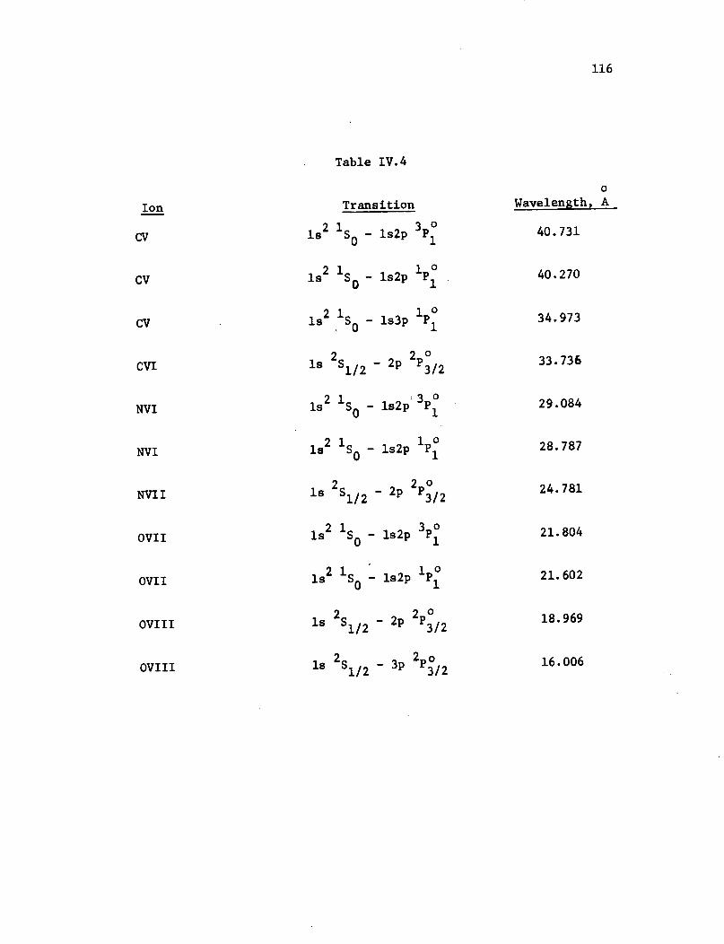
116
Table IV.4
Transition
21 _ 3ls2 lS ls2p P1
o0 1
ls2 lS0- ls3p P1
21 2 °is 1 S -ls2p P1
21 °
ls 1S - ls2p 1p
2 20
is 21/2 - 2p P3 /2
ls2 1 S -ls2p 3p0
21 1
is S -ies2p 10
ls 21/2 - 2p P3/2
121 2
is 2S1/2 - 3p /2
0
Wavelength, A
40.731
40.270
34.973
33.736
29.084
28.787
24.781
21.804
21.602
18.969
16.006
Ion
CV
CV
CV
CVI
NVI
NVI
NVI I
OVII
OVII
OVIII
OVIII
117
Solving equation (4.36) for a,
T 2 (4.37)2 R
and using the trigonometric identity for the sin of the difference
of two angles gives
sin B = cos k (4.38)
The difference in the wavelength calculated and the published wave-
length of the line never exceeded +0.05 A over the range of interest
so that the calculated wavelengths of the satellites should be
within this accuracy.
An attempt to record the intensity, as a function of time, of
the satellite and the resonance lines was made. To this end the
film holder assembly was removed from the grazing incidence spectro-
graph and replaced by two photoelectric detectors. These detectors
consisted of a thin plastic scintillator (Naton 136) coated with a
thin aluminum film on both sides. The edge of the scintillator
served as the exit slit, while the aluminum coating prevented light
loss out of the sides. The back edge of the scintillator was opti-
cally coupled to a glass fiber light guide by a drop of high-
viscosity silicone oil. The other end of the light guide was placed
in front of the photocathode of an Amperex 150 APV photomultiplier
which was isolated from the vacuum chamber by a quartz (SiO2) window.
118
While it was possible to obtain time resolved signals of the radiation
in this manner (in particular the resonance lines), it was not possi-
ble to observe the satellite lines. This was due to the low inten-
sity of the lines and also due to the large amount of scattered
light at these wavelengths. The scattered light is due to the
central image which contains all wavelengths of light. The use of
filters was not possible as this reduced the intensity of the satellite
as well as the scattered light. Therefore, the effort was abandoned
and no time resolved data were obtained.
CHAPTER V
RESULTS AND CONCLUSIONS
A. Results with Boron and Carbon
Long wavelength satellites to the hydrogen-like resonance line of
carbon VI were first reported in the spectrum of a theta-pinch plasma
by Roth and Elton (1968). These lines were observed in the spectrum
produced by several discharges using deuterium as a fill gas. The
facility used in this investigation is very similar to that used by
these authors and was expected to produce a reasonably similar plasma
(i.e., same electron temperature and density if operated under the
same conditions of filling pressure and main bank energy). Thus,
the reasonable starting point for this investigation was to obtain a
spectrum under the same experimental conditions as those used by
Roth and Elton (1968). Carbon along with other impurities such as
oxygen and silicon are always present in the discharge. The carbon
is due to vacuum pump oil (a hydrocarbon compound) which manages to
"backstream" past the liquid nitrogen cold trap between the vacuum
pump and the quartz (SiO2) tube containing the gas. Over a period of
several hours of pumping, the oil is deposited on the walls of the
quartz tube and is injected into the plasma along with the silicon
and oxygen during the preheating phase. The spectrum obtained
therefore contained carbon lines with very good intensity. 'After the
film on which the spectrum was recorded had dried, it was scanned
pRCEDNG PAG BLNN . 120
on a Joyce-Loebl microdensitometer at a 50 to 1 scanning ratio so
that the distance between a given pair of lines was 50 times as
great on the recording as on the film. The microdensitometer employs
a single lamp to measure alternatively the transmission of the film,
and the transmission of a calibrated density wedge so that the photo-
metric density D is therefore recorded. While a spectrum was being
scanned on the microdensitometer, the spectral region of interest
was visually monitored through a magnifying glass to insure that all
weak lines were recorded and noted. The microdensitometer recording
of the film obtained with deuterium is shown in Figure 16. The
tracing shows 11 lines (Roth and Elton reported nine, one of which
was observed only in second order) to the long wavelength side of
0the carbon VI resonance line at 33.734 A and lying between it ando
2 1p o o0the ls S - ls3p P transition of carbon V at 34.973 A. The0 1
measured wavelengths of these lines are included on Figure 16 along
with the composition and initial pressure of the fill gas, as well
as the electron temperature estimated by the method discussed in
Chapter IV. The agreement between the observed wavelengths and the
calculated wavelengths of the satellites is in remarkably good
agreement. However, three of the observed lines correspond to
satellite transition where the upper (doubly excited) state cannot be
formed by inverse autoionization, as the process is forbidden by
parity. A comparison between these measured and calculated values
is given in table V.1.
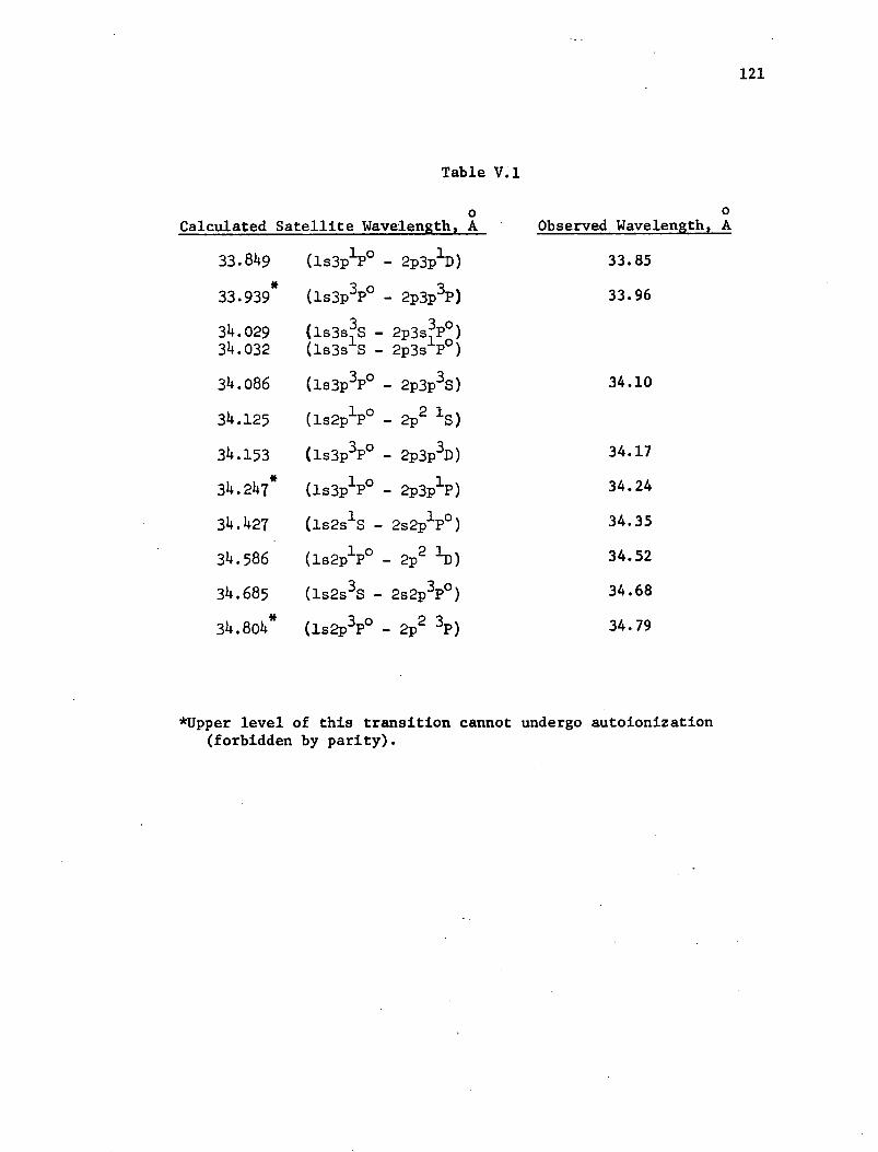
121
Table V.1
oCalculated Satellite Wavelength, A
33.849 (ls3pP° - 2 p3plD)
33-939 (ls3p3p° - 2p3p3 p)
34.029 (ls3s3S - 2p3s3Po)34.032 (ls3s S - 2p3s P° )
34.086 (ls3p3P° - 2p3p3S)
34.125 (ls2plpO - 2p2 1S)
34.153 (ls3p3 PO - 2p3p3D)
34.247 (ls3p lp - 2 p3p P)
34.427 (1s2slS - 2s2plp ° )
34.586 (ls2plpO - 2p2 1D)
34.685 (ls2s3 S - 2s2p3 P0)
34.804* (ls2p3 pO - 2p2 3 p)
0
Observed Wavelength, A
33.85
33.96
34.10
34.17
34.24
34.35
34.52
34.68
34.79
*Upper level of this transition cannot undergo autoionization(forbidden by parity).
122
The intensities of these observed lines, however, were too low
to allow photoelectric recording which was required in order to
investigate the time history of the line intensities. This part of
the investigation was required in order to determine the stage of
ionization responsible for the formation of the doubly excited states
since the doubly excited state could be formed by inverse auto-
ionization involving free electrons and hydrogen-like ions or by
collisional excitation of both electrons of the helium-like ion.
This latter process is less likely since much more energy is in-
volved than in the formation from a free electron and a hydrogen-like
ion. The concentration of the hydrogen-like and the helium-like
ions would be a maximum at different temperatures and, for the tran-
sient plasma in the theta-pinch, at different times. This is borne
out by Figure 2 which shows the temperature dependence of the carbon
ions. Thus if the doubly excited state were formed by inverse auto-
ionization the intensity of the satellite would reach a maximum when
the number of hydrogenic ions is a maximum. This maximum number of
hydrogenic ions would be indicated by a maximum intensity of the
hydrogenic resonance line as indicated by equation (3.63). Thus
if,as expected,inverse autoionization were the mechanism by which
the doubly excited states were formed the satellite intensity should
reach a maximum simultaneously with the hydrogenic resonance line.
If, on the other hand, the doubly excited states were formed by
collisional excitation in helium-like ions (which is less likely)
123
the satellite intensity would reach a maximum when the concentration
of helium-like ions is a maximum. This maximum would be indicated
by a maximum in the intensity of the helium-like resonance line.
Thus if collisional excitation were responsible for the formation
of the doubly excited states the satellite intensity should reach a
maximum simultaneously with the helium-like resonance line.
Furthermore, collisional excitation should lead to the formation of
doubly excited states which cannot autoionize and therefore cannot
be formed by inverse autoionization so that if collisional processes
were important satellites corresponding to transitions from these
states should be observed. In fact, three wavelengths (33.939 A,
o o34.247 A, and 34.804 A) which were calculated for such transitions
were observed; however, this did not mean that all lines were formed
by collisional processes. The percentage of carbon in the deuterium
fill gas was increased to 2.5 percent by the addition of acetylene
(C2H2). The microdensitometer recording of the satellite lines
obtained on this film is shown in Figure 17. The interesting result
obtained is that there is no apparent increase in the intensity of
the satellites over the previous spectrum obtained with only deuterium,
even though there was a noticeable increase in the other carbon
0lines (about a factor of two for the CV line at 34.973 A). A third
spectrum taken with the carbon concentration increased to 5 percent
produced the same peculiar result of increasing the intensity of the
normal carbon lines but with not apparent effect on the satellite
intensities. Higher concentrations of carbon were not attempted as
124
impurity concentrations above this level were found to result in a
lower temperature plasma.
While the above result was surprising it did not prove conclu-
sively that the lines were not due to carbon. The rate coefficient
for dielectronic recombination was examined to determine if the above
result could be explained in terms of its temperature dependence.
An approximate general formula for the total rate coefficient Kd
has been derived by Burgess (1965b)
Kd = T 3/2 f(q,p)exp (- E(q,p) cm3sec (51)
e p
where f(q,p) is the oscillator strength and E(q,p) the energy of
the transition q - p with q the initial state of the recombining
ion. The function 4 is separable into two slowly varying functions
of Z, the charge of the recombining ion and of X = (Z + 1)2
Eq,p
respectively, where e (Z + 1)2 is defined as the energy inq,p
Rydbergs of the transition p + q. The summation is carried out
over all excited states p of the recombining ion, of which the
first is usually the most important (Goldberg, 1966). Using this
approximate formula, Goldberg (1966) derives the temperature at which
Kd
has its maximum value. Goldberg obtains the relation
T = 0.96v K (5.2)max
125
where v is the frequency of the resonance line of the recombining
ion in wavenumbers. Thus the simple rule for estimating the tempera-
ture at which dielectronic recombination is most effective(it can be
much greater than radiative recombination) is to take the temperature
equal to the wavenumber of the resonance line of the recombining ion.
Using this estimate one would expect dielectronic recombination to
be most- important for carbon VI at a temperature of 2.96 x 10⁶ OK
(255.2 eV) which is slightly higher than the electron temperature
obtained in the theta-pinch plasma if dielectronic recombination is
ignored. Therefore, boron was chosen as the next element to be
0oinvestigated since the resonance line of boron V at 48.587 A pre-
6odicts a temperature of 2.06 x 10 K (177.6 eV) at which dielectronic
recombination should be a maximum. This temperature is at the lower
end of the electron temperature range produced in the theta-pinch.
Boron was introduced into the experiment in the form of diborane
(B2H6) gas. This gas was only available as a mixture of diborane and
hydrogen with a maximum concentration of diborane of 10% (this con-
centration is set by the Interstate Commerce Commission). Thus the
maximum concentration of boron was limited to 2.5%. The micro-
densitometer recording of the spectral region on the long wavelength
side of the boron V resonance line obtained from this set of condi-
tions is shown in Figure 18. The region containing the calculated
o osatellite wavelengths (48.743 A to 50.118 A) contains only three
lines, only two of which correspond in wavelength to the calculated
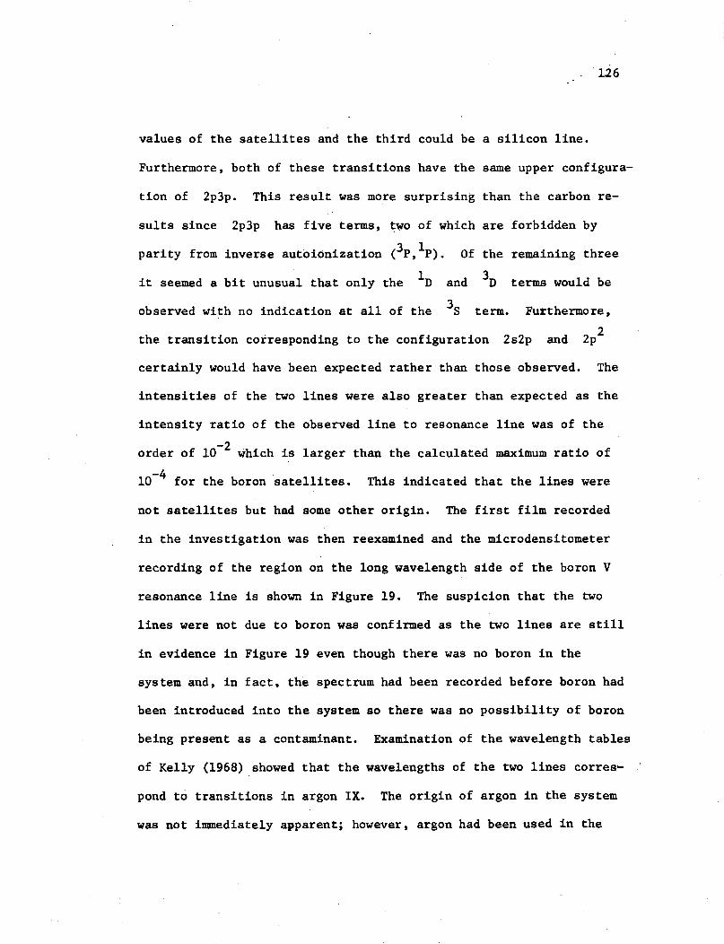
126
values of the satellites and the third could be a silicon line.
Furthermore, both of these transitions have the same upper configura-
tion of 2p3p. This result was more surprising than the carbon re-
sults since 2p3p has five terms, two of which are forbidden by
parity from inverse autoionization (3p,1p). Of the remaining three
it seemed a bit unusual that only the 1D and 3D terms would be
observed with no indication at all of the 3S term. Furthermore,
the transition corresponding to the configuration 2s2p and 2p2
certainly would have been expected rather than those observed. The
intensities of the two lines were also greater than expected as the
intensity ratio of the observed line to resonance line was of the
order of 10- 2 which is larger than the calculated maximum ratio of
10- 4
for the boron satellites. This indicated that the lines were
not satellites but had some other origin. The first film recorded
in the investigation was then reexamined and the microdensitometer
recording of the region on the long wavelength side of the boron V
resonance line is shown in Figure 19. The suspicion that the two
lines were not due to boron was confirmed as the two lines are still
in evidence in Figure 19 even though there was no boron in the
system and, in fact, the spectrum had been recorded before boron had
been introduced into the system so there was no possibility of boron
being present as a contaminant. Examination of the wavelength tables
of Kelly (1968) showed that the wavelengths of the two lines corres-
pond to transitions in argon IX. The origin of argon in the system
was not immediately apparent; however, argon had been used in the
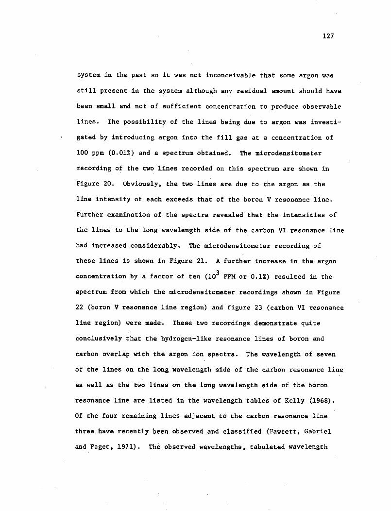
127
system in the past so it was not inconceivable that some argon was
still present in the system although any residual amount should have
been small and not of sufficient concentration to produce observable
lines. The possibility of the lines being due to argon was investi-
gated by introducing argon into the fill gas at a concentration of
100 ppm (0.01%) and a spectrum obtained. The microdensitometer
recording of the two lines recorded on this spectrum are shown in
Figure 20. Obviously, the two lines are due to the argon as the
line intensity of each exceeds that of the boron V resonance line.
Further examination of the spectra revealed that the intensities of
the lines to the long wavelength side of the carbon VI resonance line
had increased considerably. The microdensitometer recording of
these lines is shown in Figure 21. A further increase in the argon
concentration by a factor of ten (103 PPM or 0.1%) resulted in the
spectrum from which the microdensitometer recordings shown in Figure
22 (boron V resonance line region) and figure 23 (carbon VI resonance
line region) were made. These two recordings demonstrate quite
conclusively that the hydrogen-like resonance lines of boron and
carbon overlap with the argon ion spectra. The wavelength of seven
of the lines on the long wavelength side of the carbon resonance line
as well as the two lines on the long wavelength side of the boron
resonance line are listed in the wavelength tables of Kelly (1968).
Of the four remaining lines adjacent to the carbon resonance line
three have recently been observed and classified (Fawcett, Gabriel
and Paget, 1971). The observed wavelengths, tabulated wavelength
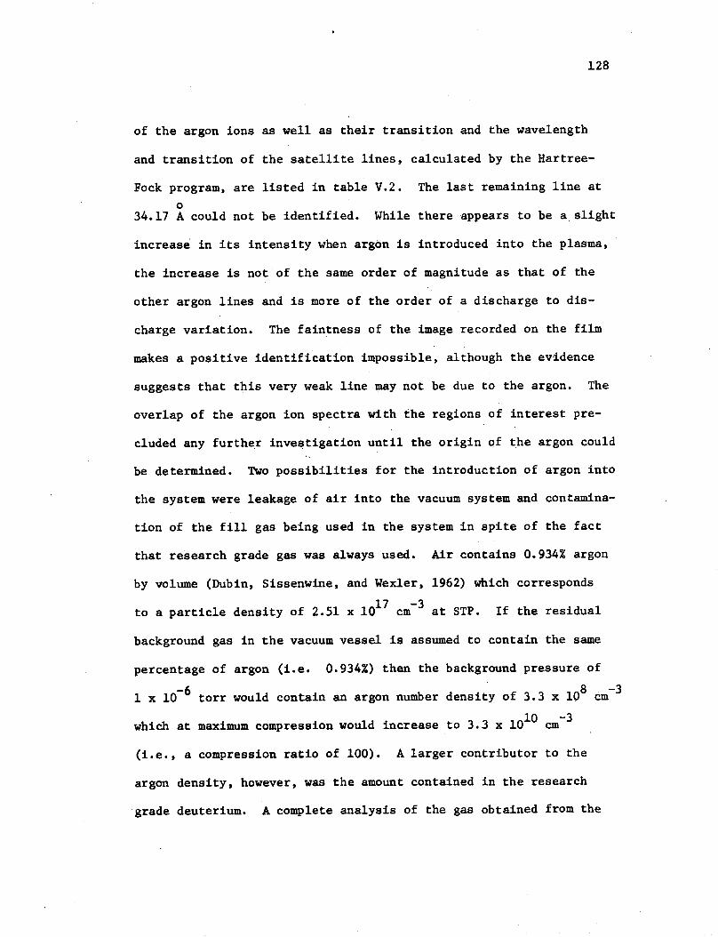
128
of the argon ions as well as their transition and the wavelength
and transition of the satellite lines, calculated by the Hartree-
Fock program, are listed in table V.2. The last remaining line at
034.17 A could not be identified. While there appears to be a slight
increase in its intensity when argon is introduced into the plasma,
the increase is not of the same order of magnitude as that of the
other argon lines and is more of the order of a discharge to dis-
charge variation. The faintness of the image recorded on the film
makes a positive identification impossible, although the evidence
suggests that this very weak line may not be due to the argon. The
overlap of the argon ion spectra with the regions of interest pre-
cluded any further investigation until the origin of the argon could
be determined. Two possibilities for the introduction of argon into
the system were leakage of air into the vacuum system and contamina-
tion of the fill gas being used in the system in spite of the fact
that research grade gas was always used. Air contains 0.934% argon
by volume (Dubin, Sissenwine, and Wexler, 1962) which corresponds
17 -3to a particle density of 2.51 x 10 cm at STP. If the residual
background gas in the vacuum vessel is assumed to contain the same
percentage of argon (i.e. 0.934%) then the background pressure of
1 x 10- 6
torr would contain an argon number density of 3.3 x 108 cm-3
which at maximum compression would increase to 3.3 x 1010 cm- 3
(i.e., a compression ratio of 100). A larger contributor to the
argon density, however, was the amount contained in the research
grade deuterium. A complete analysis of the gas obtained from the
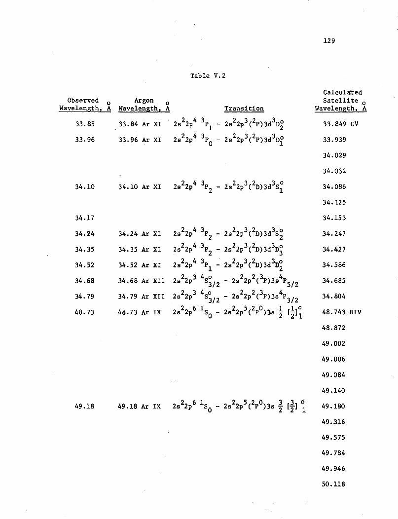
129
Table V.2
ObservedWavelength, A
33.85
33.96
34.10
34.17
34.24
34.35
34.52
34.68
34.79
48.73
Argon oWavelength, A
33.84 Ar XI 2s22p4 3P
33.96 Ar XI 2s22p4 3P00g
34.10 Ar XI
34.24 Ar
34.35 Ar
34.52 Ar
34.68 Ar
34.79 Ar
48.73 Ar
XI
XI
XI
XII
XII
IX
Transition
2s2 2p3 (2p)3d3 Do
- 2s2 2p3 (2p)3d3 Do
2s22p4 3P2 - 2s2 2p3 (2 D)3d3 S0
2s22p4
2s22p4
2s22p 4
2s22p3
2s 2 2p 3
2s22p6
3P -2
3 p -2
3p -1
4oS3 / 2
40S3/2
lS -
2s22p3(2 D)3d3S;
2s2 2p3 (2D)3d3D2
2s2 2p3(2D)3d
3D
- 2s22p2(3p )3s4P
- 2s22p2(3P)3s4P3/ 2
2s 2 2p 5 (2pO)3s 1 [110
CalculatedSatellite 0
Wavelength, A
33.849 CV
33.939
34.029
34.032
34.086
34.125
34.153
34.247
34.427
34.586
34.685
34.804
48.743 BIV
48.872
49.002
49.006
49.084
49.18 Ar IX 2s22p6 1S0 2s22p5(2p0)3s 3 32 149.18
49.140
49.180
49.316
49.575
49.784
49.946
50.118
130
supplier (The Matheson Company) showed an argon concentration of 15
PPM. This concentration amounts to a particle density of 3.3 x 10¹²
-3cm , that is, two orders of magnitude greater than the background
gas. The intensity of a typical argon ion line in the wavelength
region of interest was estimated with the assumption that only two
ionization stages of argon existed (AXI and AXII) and using only the
concentration of argon in the deuterium fill gas (since the contri-
bution of argon in the residual background gas in the vacuum vessel
would contribute only one percent of the argon and could be ignored
without affecting the accuracy of the estimate). The ratio of A XII
ions to A XI ions was determined from equation (4.18) ignoring di-
electronic recombination. At an electron temperature of 200 eV the
ratio is
n (A XII) = 16.5 (5.3)n (A XI)
If the effects of dielectronic recombination were included a
slightly lower ratio would result in equation (5.3). However, the
work of Burgess and Summers (1969) suggest that the correction would
be small and well within the approximations made in obtaining the
value in equation (5.3). Since the sum of the argon XI and argon
XII number density is assumed to equal the total density of argon,
the argon XII number density is
n(A XII) z 3 x 10 cm (5.4)
131
The argon XII line radiation in the region of interest consists of
transition to the ground state at a wavelength which corresponds to
the transition from the doubly excited state in carbon V. Thus,
the excited argon XII level lies approximately 360 eV above the
ground state. The absorption oscillator strength for the argon XII
transition was estimated to be 0.3 by use of the Coulomb approximation
of Bates and Damgaard (1949). The rate coefficient for collisional
excitation K(l,q) (equation (3.18))was then evaluated using the
above values of f(l,q) and E(l,q) and an electron temperature of
200 eV. The results
K(l,q) z 1 x 10⁻⁸ cm3 sec (5.5)
was then substituted in equation (3.43) to obtain an expression for
the number density in the excited state
n() e A(q)10 (5.6)n(l) A(q)
Taking the upper state of the argon XII transition as the first
excited level (i.e., the only allowed spontaneous transition is to
the ground level) and using the previously discussed values of
n(A XII) and ne, the number density of excited levels becomes
221022 -3
n(2) cm10 (5.7)A(2,l) c
132
Using equation (3.65) for the intensity of the satellite line and
equation (3.47) for the intensity of the argon XII line the intensity
ratio of argon XII to satellite is approximately
I(A XII) 10 22
I(sat.) ~ Ad(p,q)n(d )
The number density of doubly excited states in carbon V for a 5%
concentration of carbon was determined from the Saha-Boltzmann
equation [equation (3.36)] since this gives a maximum, with plasma
condition of kT = 200 eV and n = 2.2 x 10 cm . The Saha-e e
Boltzmann equation predicts for these conditions
n(d) S 1011 cm- 3 (5.9)
The calculations of oscillator strengths as discussed in Chapter II
show that the transition probability for a typical carbon satellite
10 -lis of the order of 10 sec 1 . Using this value the intensity ratio
of argon XII to carbon VI satellite becomes
I(A XII) 101 > 10 (5.10)I(sat.)
Thus the intensity of the argon XII line due to the contamination in
the fill gas would exceed the intensity of the satellite by a factor
of 10 if the number density of doubly excited states is its
133
equilibrium value. However, it has been pointed out that the life-
time of the doubly excited state to radiative decay is of the same
order of magnitude as the time between electron collision and there-
fore it would be expected that the population of the doubly excited
states would be below the equilibrium value. This condition was
verified experimentally by the installation of a deuterium gas
purifier. This purifier consisted of a palladium-silver element
heated electrically. The palladium-silver alloy has the unique
property of allowing only hydrogen (and its isotope deuterium) to
pass through a thin wall constructed of the alloy. Thus any element
heavier than deuterium is removed from the gas and only ultrahigh
purity deuterium is fed into the vacuum system. The purifier used
was constructed by the National Bureau of Standards (Gaithersberg,
Md.) and purifies hydrogen of 95% purity to a purity level which
could not be determined. A microdensitometer recording of a spectrum
obtained with the purified deuterium is shown in Figure 24. The
recording covers the region to the long wavelength side of the carbon
VI resonance line and shows a conspicuous absence of satellite lines.
A careful comparison of Figure 24 and Figure 16 shows that, at most,
only three lines are faintly visible. It was not anticipated that
the lines would disappear completely, as the concentration of argon
due to leakage of air into the vacuum system could not be eliminated.
That these three lines were not satellites was confirmed by the
addition of carbon to the system (up to 5%) with no observed increase
in their intensity.
134
The establishment of detectable intensity ratios also indicated
that the lines which were observed could not be satellites. The
limit of detectability was determined (for the film used) by calcu-
lating the intensity ratio of the weakest detectable line in the
region of interest,to the carbon VI resonance line. It was assumed
that the film had a linear response as discussed in Chapter IV and
the profile of each line was assumed to be triangular. This ratio
indicated that an intensity ratio of about 10-
3 could be detected
with certainty (which is about the maximum value for carbon at
temperature of 200 eV.) This limit was due to saturation of the
emulsion at the resonance line center and increasing the exposure
in order to increase the detectability of weak lines prevented the
determination of the recorded resonance line intensity and did not
show any satellites. Thus it was concluded that the transitions
involving doubly excited states were not observable under the
experimental conditions and that even if the satellites would have
appeared with a reasonable intensity the overlap of the argon ion
spectra would have rendered these two cases (boron and carbon) as
unsuitable for further investigation.
B. Results with Nitrogen
Since carbon and boron were shown to be unacceptable elements for
the experiment, the last element, nitrogen, which was feasible to
investigate in this experiment due to the accessability of the
hydrogen-like resonance line and since it was possible to produce
the hydrogen-like ion,--was introduced-into the plasma using the ultra
135
high purity (using the palladium leak) deuterium as a fill gas. The
research grade nitrogen which was used contained about 5 PPM of
argon but since the percentage of nitrogen introduced into the sys-
tem would be small (a maximum of 3% N2 or 6% N) the total amount
of argon introduced into the system would only be about 0.3 PPM
9 -3which would correspond to a particle density of about 7 x 10 cm
which is less than the concentration of argon in the residual gas
in the vacuum vessel. Figure 25 is the microdensitometer recording
of the spectrum obtained with 1% N2 added to the fill gas. The
recording covers the region to the long wavelength side of the N VII
oresonance line at 24.781 A. Two lines are visible in the region and
their wavelengths are in resonable agreement with the calculated
values of two of the satellites. However, the intensity ratio of
the observed line to resonance line was found to be approximately
7.5 x 10- 2 (as determined by the method of the previous section)
which is larger than the maximum value calculated for the satellites
(even if the values obtained by Gabriel and Paget (1972) are used.)
Spectra at high concentration of N2
(2% and 3%) were obtained and
the microdensitometer recordings of the region are shown in Figures
26 and 27. The two lines are obvious in both of these recordings
and the ratio of observed line to resonance line in each case is
the same as that obtained for the first case. This large intensity
ratio could not be resolved in the light of dielectronic recombination
and it was therefore concluded that the two lines were not due to
transition from doubly excited states but were more likely to be due
136
to a contamination in the gas. Argon XII lines at approximately
these wavelengths have recently been identified by Fawcett, Gabriel,
and Paget (1971) and it was concluded that these lines most likely
were due to the argon contamination in the background gas. This
result was finally verified after extensive work on the vacuum
system which improved the base pressure to about 10- 8
torr. Spectra
recorded under these conditions with 1% N2added showed that the
two lines were not produced and that no satellite lines existed
with sufficient intensity to be recorded. This situation existed
even for a spectra recorded with as many as six discharges on
a single film, even though the emulsion saturated at the center of the
resonance line. Table V.3 compares the observed wavelengths with the
calculated values of the satellite as well as the reported wavelengths
of the argon ions.
C. Conclusions and Limits of Laboratory Experiments
Laboratory observation of transitions from doubly excited states
in two electron ions does not appear to be very compatible with
experimental devices such as the theta-pinch, the limiting factor
being, of course, the low intensity of the spectral lines emitted in
the transition from the doubly to the singly excited state. The
experimental evidence indicates that even under the best conditions
the detectability of the lines would not be possible in such an
experiment with the photographic methods employed here. Even
resorting to multiple exposures in order to increase the density on
the film failed to show any evidence of satellites. This was due to
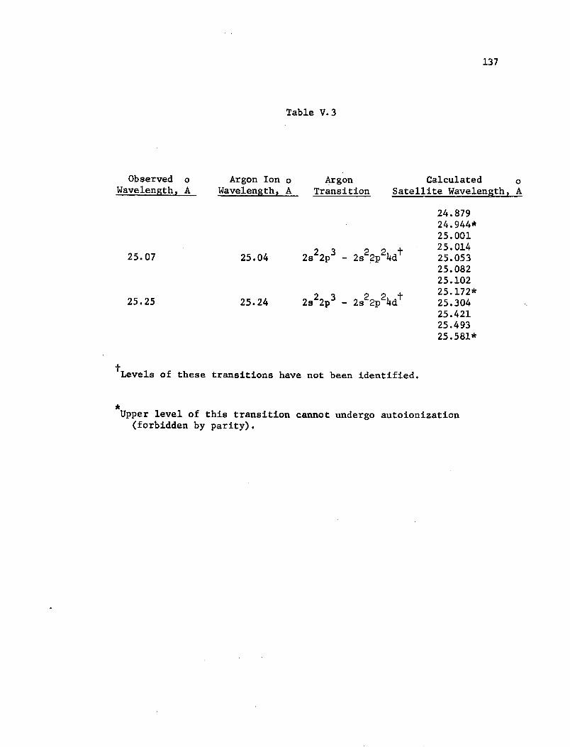
137
Table V.3
Observed oWavelength, A
Argon Ion oWavelength, A
ArgonTransition
Calculated oSatellite Wavelength, A
25.04
25.24
2s2 2 p 3 - 2s22p24dt
2s2 2p3 - 2s22p24dt
24.87924.944*25.00125.01425.05325.08225.10225.172*25.30425.42125.49325.581*
Levels of these transitions have not been identified.
Upper level of this transition cannot undergo autoionization(forbidden by parity).
25.07
25.25
138
the increase in the film background density due to continuum emission
as well as scattered light from the central image (this is particu-
larly bad in grazing incidence mountings when looking at the shorter
wavelengths). Furthermore, the satellites are situated close to the
resonance line so that increasing the exposure would increase the
film density corresponding to the intensity in the wings of the line
which in turn is another contribution to the film background. A min-
imum intensity ratio of satellite to resonance line of about 10-
3
would be required for the satellites to be detectable with the photo-
graphic method used here. This is the maximum value calculated with
the assumption of the doubly excited states being populated to their
equilibrium value and even if this value were obtainable it would
impose severe restrictions on such an experiment. There was, there-
fore, no experimental evidence to indicate that the process of di-
electronic recombination is important in the theta-pinch since no
lines which could be conclusively identified as true satellites were
observed. This does not imply that such lines are not emitted in the
plasma, but it does limit the intensity such a line would have which,
at best, is of the same order of magnitude as the background noise.
These conclusions also apply to previous experimental work in this
field in which a high temperature discharge has been used to observe
"satellites". In particular, in the experiments of Roth and Elton
(1968) a theta-pinch device was used with essentially the same filling
gas and electrical properties, since the design of the present experi-
mentis very close to that of NRL, Washington. The correspondence
between the lines identified here as argon and the fact that they
made no special efforts to obtain pure filling gas indicate that their
139
identifications are in error. In addition, early work by Gabriel and
Jordan (1969) who also used a theta-pinch was also incorrect for the
same reasons. This has been confirmed by Gabriel (1971) (private
communication).
However, recently Gabriel and Paget (1972) have reported the
observation of satellites to the helium like resonance lines of
nitrogen and oxygen in a theta-pinch. Their intensities ratios were
of the order of their calculated values (i.e., a factor of 2 or 3
higher than the values calculated here). Wnile oxygen satellites
were not investigated in this experiment the results of Gabriel and
Paget (1972) with nitrogen indicates that the failure to observe
satellites in this experiment should have some reasonable explanation.
The most probable explanation is based on the inverse temperature
dependence of the intensity ratio. In the experiment discussed here
the effect of dielectronic recombination was not taken into account
in the calculation of the ionization balance required in the tempera-
ture determination. If this effect had been properly included or if
a more accurate temperature measurement could have been made (by
Thomson scattering) a higher temperature than the 200 eV obtained may
have been found which would decrease the intensity ratio. Further-
more, higher electron densities were obtained in this experiment (by
up to a factor of 10) which would give a smaller rate coefficient
for dielectronic recombination. Further investigation would be re-
quired in order to determine which (if not both) of the two factors
were responsible for the null result obtained.
Our conclusions that there is as yet no absolutely firm
laboratory evidence for the formation of "satellites" by the process
140
of dielectronic recombination, does not mean that it is not an
important astrophysical process. In fact, the circumstantial evi-
dence from ionization balance is very convincing. However, the
change overlap of argon with other spectra, as reported in this work,
indicates that the identification of observed "satellites" in solar
spectra (Fritz, et al., 1967; Rugge and Walker 1968; Jones, Freeman
and Wilson 1968; Walker and Rugge, 1970) should be closely examined
and the relative intensities carefully checked.
D. Suggestions for Future Work
The use of laboratory experiments to investigate the processes
of dielectronic recombination still warrants further consideration.
While the use of plasma devices such as theta-pinch for the investi-
gation does not appear to be the most profitable due to lack of ob-
servation of the satellite lines for the case investigated here,
other devices may be able to make a contribution in this area. The
device commonly referred to as a sliding spark (Conrads and Hartwig,
1964), having a lower temperature than the theta-pinch (since R is
proportional to T ) could be advantageous although the higher den-
sity could be a disadvantage. In fact, satellite lines of carbon
were first observed in a spark device (Edlen and Tyren, 1939) however,
it is not clear whether dielectronic recombination or electron-exci-
tation forms the doubly-excited states. While the diagnostics of
such a device would be considerably more difficult, an investigation
of the observed satellites in such a device should be carried out.
Low temperature plasma devices in conjunction with a higher energy
electron beam to excite the ions of interest would probably prove the
most useful for this sort of investigation.
BIBLIOGRAPHY
Allen, C. W., Astrophysical Quantities, London, The Athlone Press,1964.
Aller, L. H., The Atmospheres of the Sun and Stars, 2nd ed., New York,Ronald Press Company, 1963.
Bates, D. R., and Damgaard, A., Phil. Trans. Roy. Soc. London A, 242,101, 1949.
Bates, D. R., and Dalgarno, A., "Electronic Recombination" in Atomicand Molecular Processes, ed. Bates, D. R., New York, AcademicPress, 1962.
Beerwald, H., Bogen, P., El-Khalafawy, T., Fay, H., Hintz, E., andKever, H., Nucl. Fusion Supp. part II, 595, 1962.
Beutler, H. G., J. Opt. Soc. Am. 35, 311, 1945.
Bodin, H. A. B., Green, T. S., Niblett, G. B. F., Peacock, N. J.,Quinn, J. M. P., and Reynolds, J. A., Nucl. Fusion Supp. part II,521, 1962.
Bohr, N., Z. Physik 9, 1, 1922.
Brown, F. W., Phys. Rev. 44, 214, 1933.
Burgess, A., and Summers, H. P., Ap. J. 157, 1007, 1969.
Burgess, A., "Dielectronic Recombination," The Formation of SpectrumLines. Proceedings 2nd Harvard-Smithsonian Conference onStellar Atmospheres, Cambridge, Smith. Astr. Obs. Spec. Rept.No. 174, 1965a.
Burgess, A., Ap. J. 141, 1588, 1965b.
Burton, W. M., and Wilson, R., Proc. Phys. Soc. 78, 1416, 1961.
Chandrasekhar, S., Radiative Transfer, New York, Dover Publications,Inc., 1950.
Compton, K. T., and Boyce, J. C., J. Franklin Inst. 205, 497, 1928.
Condon, E. U., and Shortley, G. H., The Theory of Atomic Spectra,Cambridge, The University Press, 1963.
142
Conrads, H., and Hartwig, H. Z. Angew. Phys. 17, 188, 1964.
Conrads, H., and Oertel, G., Ap. J. 153, 975, 1968.
Cooper, J., Rep. Prog. Phys. 29, 35, 1966.
Dalgarno, A., and Parkinson, E. M., Proc. Roy. Soc. A301, 253, 1967.
Delbruick, M., Proc. Roy. Soc. A129, 686, 1930.
Dirac, P. A. M., Proc. Roy. Soc. A112, 661, 1926.
Drake, G. W. F., and Dalgarno, A., Phys. Rev. A 1, 1325, 1970.
Dubin, M., Sissenwine, N., and Wexler, H., U. S. Standard Atmosphere,Washington, D. C., U. S. Govt. Printing Office, 1962.
Edlen, B., and Tyren, F., Nature 143, 940, 1939.
Elwert, G., Z. Naturf. 7a, 432, 1952.
Evans, J. W., The Solar Corona, New York, Academic Press, 1963.
Fawcett, B. C., Gabriel, A. H., and Paget, T. M., J. Phys. B 4, 986,1971.
Fay, H., Hintz, E., and Jordan, H., "Experiments on Shock Compressionof Plasmas" in Proceedings of the Fourth International Conferenceon Ionization Phenomena in Gases, ed. Nilsson, R., Amsterdam,North Holland Publishing Co., 1959.
Feldman, U., and Cohen, L., Ap. J. 158, L169, 1969.
Flemberg, H., Ark. Mat. Astr. Fys. 28A, 1, 1942.
Fock, V., Z. f. Phys. 61, 126 1930a; Z. f. Phys. 62, 795, 1930b.
Fowler, R. H., Statistical Mechanics, Cambridge, Cambridge UniversityPress, 1955.
Fritz, G., Kreplin, K. W., Meekins, J. F., Unzicker, A. E., andFriedman, H., Ap. J. 148, L133, 1967.
Froese, C., Description of a Hartree-Fock Program with ConfigurationMixing, Univ. of British Columbia, 1965.
Gabriel, A. H., and Jordan, C., Monthly Not. Roy. Ast. Soc. 145,241, 1969.
143
Gabriel, A. H., Private Communication, 1971.
Gabriel, A. H., and Paget, T. M., J. Phys. B 5, 673, 1972.
Garstang, R. H., Class Notes , University of Colorado, Physics 656,Atomic and Molecular Spectra, 1969.
Goldberg, L., "Astrophysical Implications of Autoionization" inAutoionization, ed. Temkin, A., Baltimore, Mono Book Corp., 1966.
Goldman, L. M., Pollock, H. C., Reynolds, J. A., and Westendorp,
W. E., Phys. Rev. Letters 9, 361, 1962.
Goldman, L. M., and Kilb, R. W. C., J. Nucl. Energy C 6, 217, 1964.
Goldsmith, S., J. Phys. B 2, 1075, 1969.
Griem, H. R., Phys. Rev. 131, 1170, 1963.
Griem, H. R., Plasma Spectroscopy, New York, McGraw-Hill, 1964.
Hartree, D. R., Proc. Cambridge Phil. Soc. 24, 89, 1928.
Hartree, D. R., and Hartree, W., Proc. Roy. Soc. A150, 9, 1935.
Hearn, A. G., Proc. Sixth Conf. Ionization Phenomena in Gases, Paris,3, ed. Hubert, P., Orsay, Faculti des Sciences, 289, 1964.
Herman, F., and Skillman, S., Atomic Structure Calculations, EnglewoodCliffs, Prentice-Hall, Inc., 1963.
Hobbs , G. D., McWhirter, R. W. P., Griffen, W. G., and Jones, T. J. L.,Proc. Fifth Conf. Ionization Phenomena in Gases, Munich 2, ed.Maecker, H., Amsterdam, North Holland Publishing Co., 1965, 1962.
Jackson, J. D., Classical Electrodynamics, New York, John Wiley andSons, Inc., 1962.
Jefferies, J. T., Spectral Line Formation, Waltham, BlaisdellPublishing Co., 1968.
Jones, B. B., Freeman, F. F., and Wilson, R., Nature 219, 252, 1968.
Kelly, R. L., NRL Report 664B, 1968.
Kiang, A. T., Ma, S. T., and Wu, T. Y., Chinese J. Phys. 2, 117,1936.
Kolb, A. C., Dobbie, C. B., and Griem, H. R.,Phys. Rev. Letters 3, 1,1959.
144
Kolb, A. C., Phys. Rev. Letters 3, 5, 1959.
Kolb, A. C., Griem, H. R., Lupton, W. H., Phillips, D. T., Ramsden,S. A., McLean, E. A., Faust, W. R., and Swartz, M., Nucl.Fusion Supp. part II, 553, 1962.
Kolb, A. C., and McWhirter, R. W. P., Phys. of Fluids 7, 519, 1964.
Koopmans, T. A., Physica 1, 104, 1933.
Kramers, H. A., Phil. Mag. 46, 836, 1923.
Kunze, H. J., Gabriel, A. H., and Griem, H. R., Phys. Rev. 165, 267,1968.
Landini, M., and Fossi, B. C. M., Solar Phys. 20, 322, 1971.
Lie, T. N., and Elton, R. C., Phys. Rev. A 3, 865, 1971.
Little, E. M., Quinn, W. E., and Ribe, F. L., Phys. of Fluids 4, 711,1961.
Little, E. M., Quinn, W. E., Ribe, F. L., and Sawyer, G. A., Nucl.Fusion Supp. part II, 497, 1962.
Mack, J. E. Stehn, J. R., and Edlen, B., J. Opt. Soc. Am. 22, 245,1932.
Mees, C. E. K., The Theory of the Photographic Process, New York,The Macmillan Co., 1963.
McWhirter, R. W. P., Proc. Phys. Soc. A75, 520, 1960.
McWhirter, R. W. P., "Spectral Intensities" in Plasma DiagnositcTechniques, eds. Huddlestone, R. H., and Leonard, S. L., NewYork, Academic Press, 1965.
Namioka, T., J. Opt. Soc. Am. 49, 446, 1959.
Namioka, T., J. Opt. Soc. Am. 51, 4, 1961.
Oertel, G. K., and Williams, M. D., Rev. Sci. Instr. 36, 672, 1965.
Oertel, G. K., and Jalufka, N. W., Bull. Am. Phys. Soc. 11, 586,1966.
Pauli, Jr., W., Z. Phys. 31, 765, 1926.
Peacock, N. J., Speer, R. J., and Hobby, M. G., J. Phys. B 2, 798,1969.
145
Perrott, R. H., and Stewart, A. L., J. Phys. B. 1, 1968.
Post, R. F., J. Nucl. Energy, C, 3, 273, 1961.
Quinn, W. E., Little, E. M., and Ribe, F. L., Bull. Am. Phys. Soc. 5,341, 1960.
Roothaan, C. C. J., Revs. Mod. Phys. 23, 69, 1951.
Rose, D. J., and Clark, Jr., M., Plasmas and Controlled Fusion, NewYork, John Wiley and Sons, Inc., 1961.
Roth, N. V., and Elton, R. C., NRL Report 6638, 1968.
Rugge, H. R., and Walker, A. B. C., Space Res. 8, 439, 1968.
Runge, C. R., and Mannkopf, R., Z. Physik 45, 13, 1927.
Samson, J. A. R., Techniques of Vacuum Ultraviolet Spectroscopy,New York, John Wiley and Sons, Inc., 1967.
Sawyer, G. A., Jahoda, F. C., Ribe, F. L., and Stratton, T. F.,JQSRT 2, 467, 1962.
Seaton, M. J., "The Theory and Excitation and Ionization by ElectronImpact" in Atomic and Molecular Processes, ed. Bates, D. R.,New York, Academic Press, 1962.
Shamey, L. J., Private Communication, 1970.
Shore, B. W., and Menzel, D. H.; Ap. J. Suppl. 12, 187, 1965.
Shore, B. W., and Menzel, D. H., Principles of Atomic Spectra, NewYork, John Wiley and Sons, Inc., 1968.
Slater, J. C., Phys. Rev. 35, 210, 1930.
Slater, J. C., Phys. Rev. 81, 385, 1951.
Slater, J. C., Quantum Theory of Atomic Structure, Vol. I and II,New York, McGraw-Hill Book Co., Inc., 1960.
Spitzer, Jr., L., Physics of Fully Ionized Gases, New York, Inter-science Publishers, 1967.
Stromgren, B., Ap. J. 108, 242, 1948.
Uhlenbeck, G. E., and Goudsmit, S., Naturwiss. 13, 953, 1925.
Uhlenbeck, G. E., and Goudsmit, S., Nature 117, 264, 1926.
146
Vasilev, A. P., Dolgov-Sovelev, G. G., and Kogan, V. I., Nucl.Fusion Supp. part II, 655, 1962.
Walker, A. B. C., and Rugge, H. R., Ap. J. 164, 181, 1971.
Wilson, R., J. Quant. Spectrosc. Rad. Transfer 2, 477, 1962.
Wooley, R. v.d. R., and Stibbs, D. W. N., The Outer Layers of a Star,London, Oxford University Press, 1953.
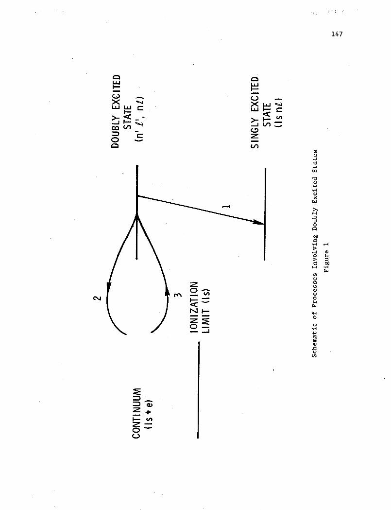
147
X0C-)
LU
0
aI-
C
C-)X u i
21)
0)
4J
cJ
>,
4-i
-I
U>
-4o
030
m
.- 4
a,
0
r.
-4
o
09w
44e
L,
CM aCO
Nfl
0-_
D ax
Z +
Z--
C_)
-4
a)wI100
-HPk
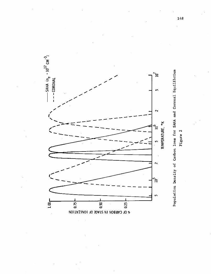
148
ca)
T~~~~~~~~~~~~~~o
o' g"o~~~~~~o
C -- ^ __
- 0
NOl IVZINOI J0 39V1S NI NOS VO 10 %
cu~~NOIIVZINOI JO JDVIS NI NO8~~~~~~~~V3 JO %c
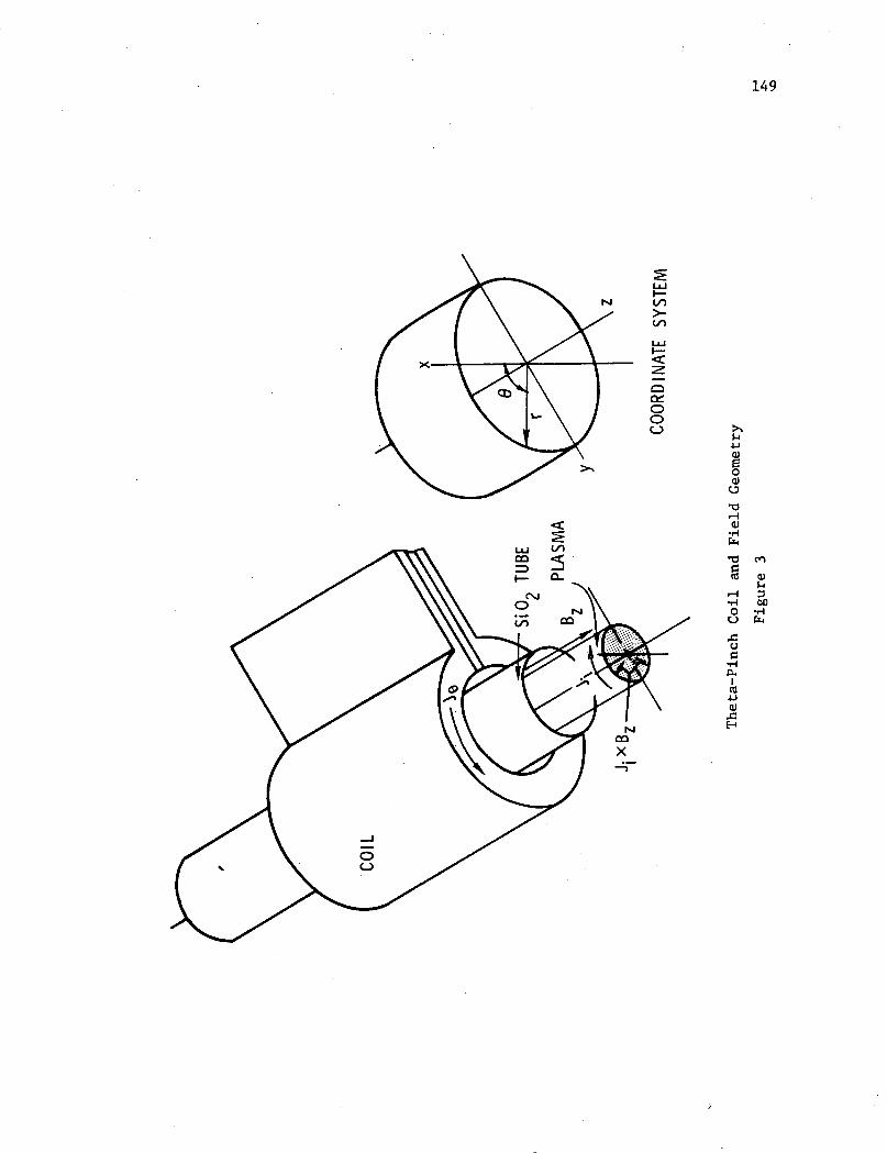
LA O
CNJ0
X
-om-0
149
i,i>-
I-
C-,
Z
00
0a)
-0 '
I-4
a)
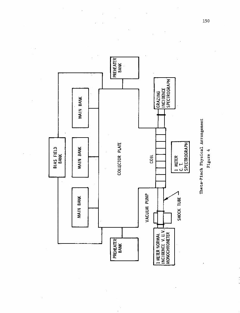
IzCLa-)0
tn F.crO.C 0u- CL
u-i
I-
0,
150
4J0
a
r.
-4
w
US
El
p.
bJ
0
F-
$4
-1
co
0
u
Ico4J
-T
0
:3boI--r4
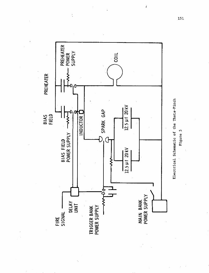
-j >
= O -D. a
LLJ~O
0-1= a
J DvL
- W
co0
An::
5Z L-
_mCI ~~ PC
c,'O
-. J.
151
0C-)
CL-
< -
,W<-
a-
CD
Nece.CL(A
o
,.,
C\icu
o
cJ
C
PI
u
4.
u
0
-.
U
44-J
0
0-I
rz4
w Z
,: ,
ZC
z L
o.1i C
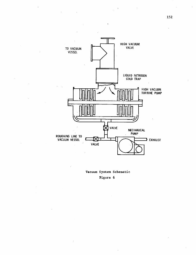
152
HIGH VACUUMVALVE
LIQUID NITROGENCOLD TRAP
ROUGHING LINE TOVACUUM VESSEL
HIGH VACUUMTURBINE PUMP
CAL
= EXHAUST
Vacuum System Schematic
Figure 6
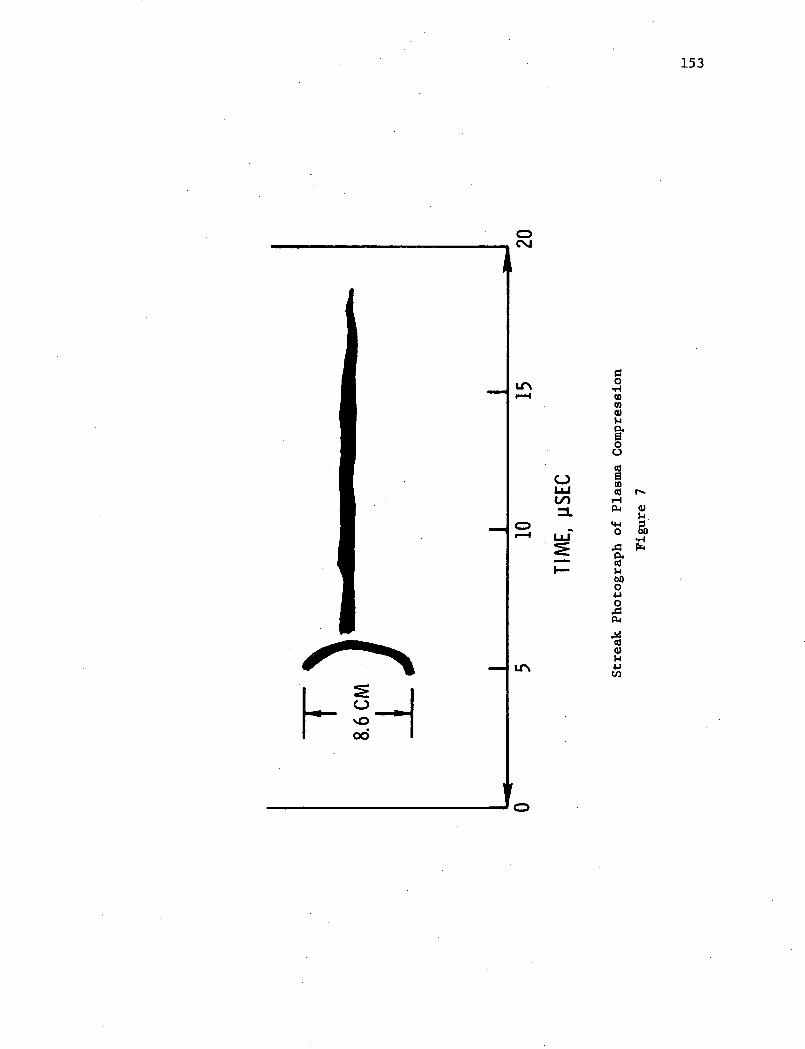
153
o
a.'4
c
I.'o r-
.4
0
PI
aLnu
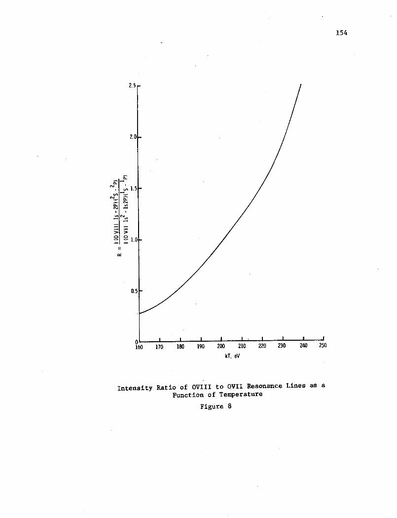
2.
Cli0.5
CL - /
0.5
0 I I I I . 1 1 , I160 170 180 190 200 210 220 230 240 250
kT, eV
Intensity Ratio of OVIII to OVII Resonance Lines as aFunction of Temperature
Figure 8
154
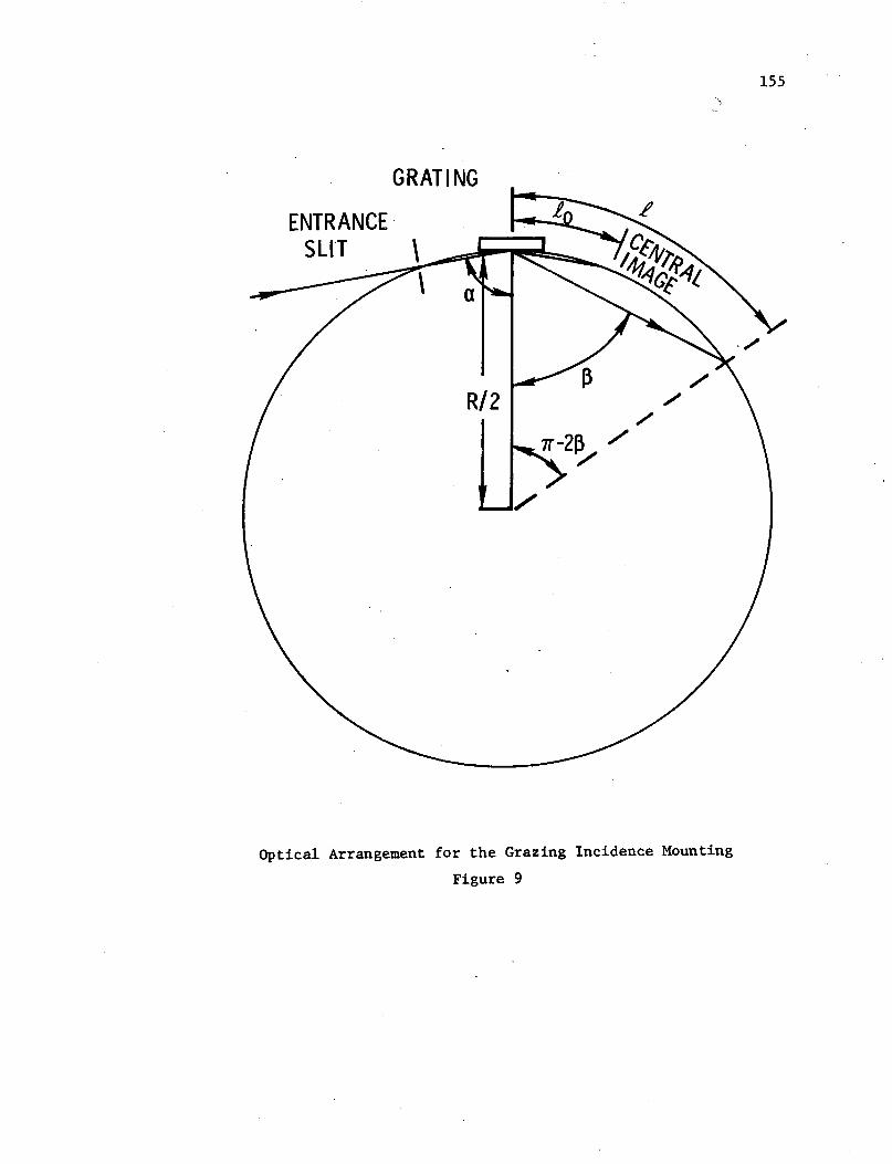
155
GRATING
Optical Arrangement for the Grazing Incidence Mounting
Figure 9
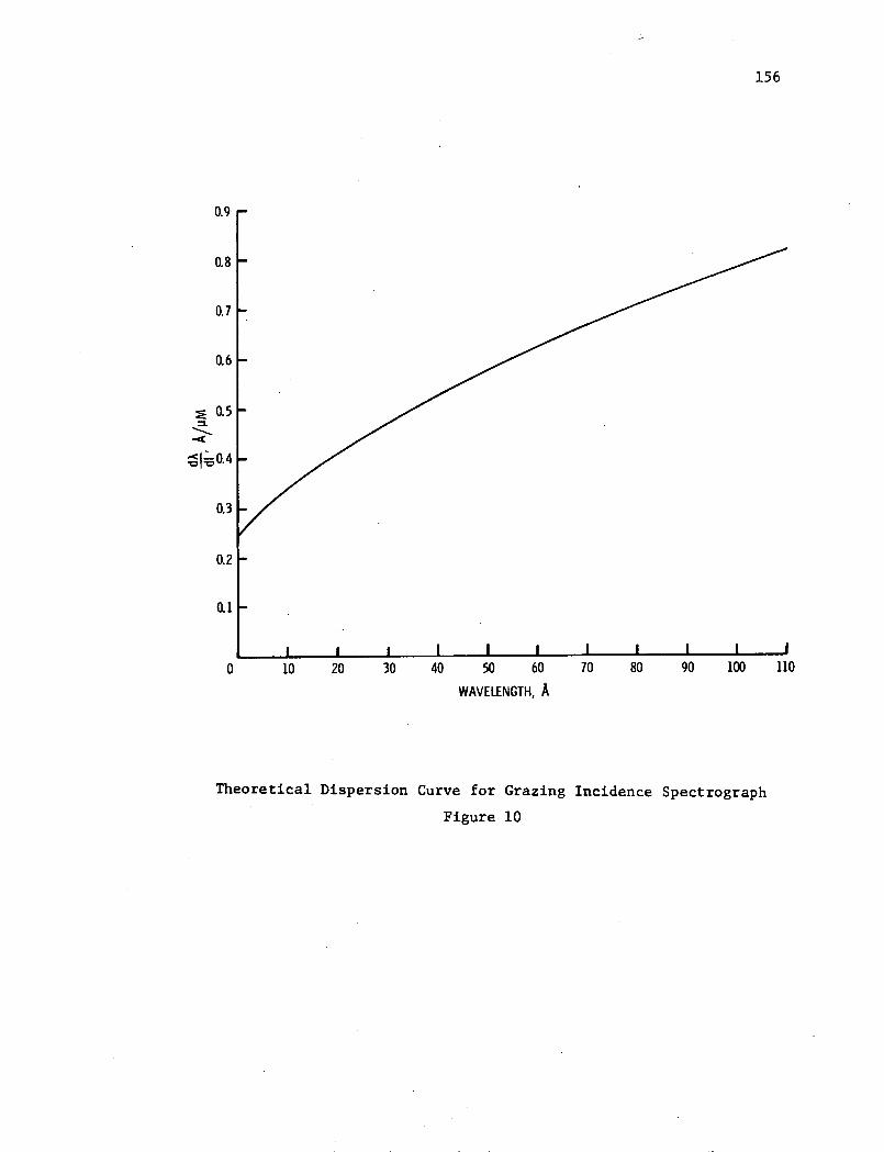
156
0.9
0.8
0.7
0.6
0.5
100.4
0.3
0.2
0.1
0 10 20 30 40 50 60 70 80 90 100 110
WAVELENGTH, A
Theoretical Dispersion Curve for Grazing Incidence Spectrograph
Figure 10
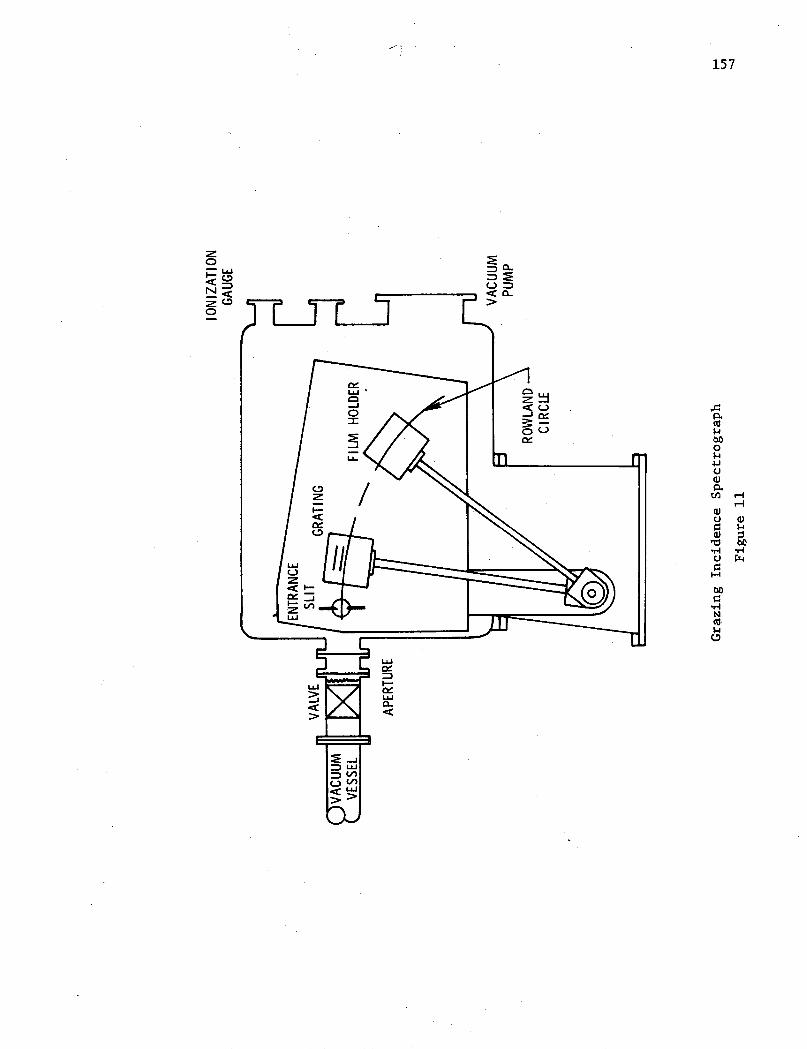
157
zo
N Z2Co
<a_
60C
-c
w
oJai
*4o
0
H1-4
bO
NC)
cis-I
.-HrZ4
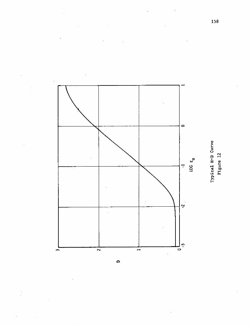
158
ucJ
I
.-
0W
olc
mC
l
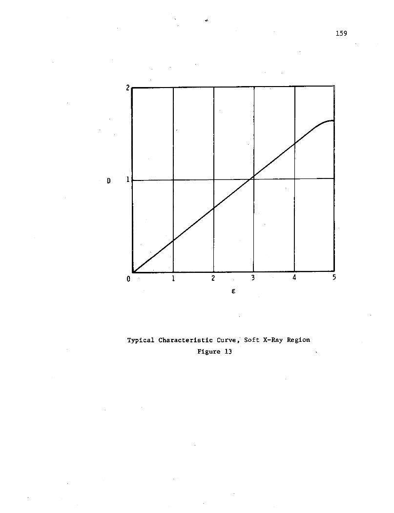
2
D 1
0 1 2 3 4
Typical Characteristic Curve,' Soft X-Ray Region
Figure 13
159
5
/~~~~~I r�
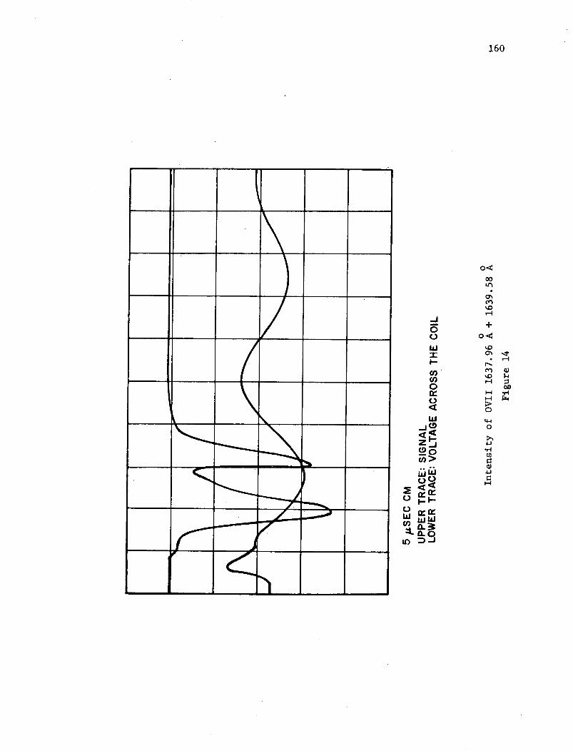
160
oto90-4u0
a%
%D--q
+
O co
nO H -~
0>-r - o
UD :-J
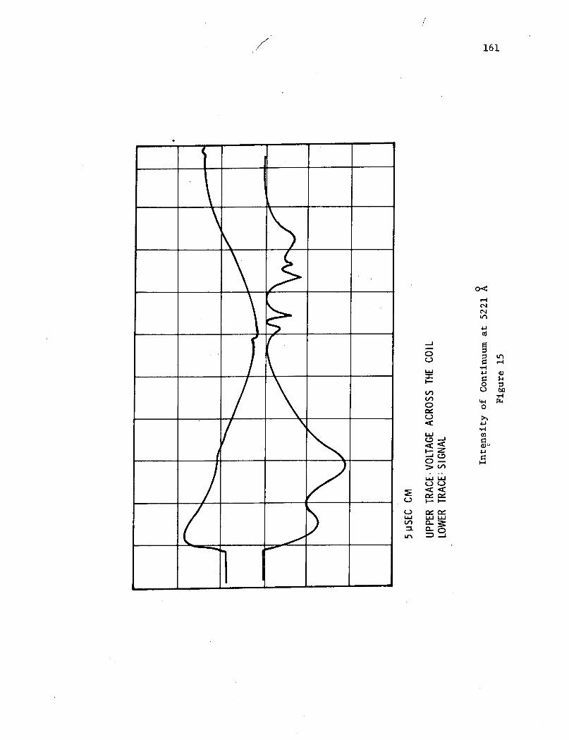
161
/
o:
04C.,
4
ul
CU
4.a-(
4J
4-i
-4
o
,--
Lo
(A1
0-2o _
Q CD
o-f Q-
Ln
-)
Wp
I-
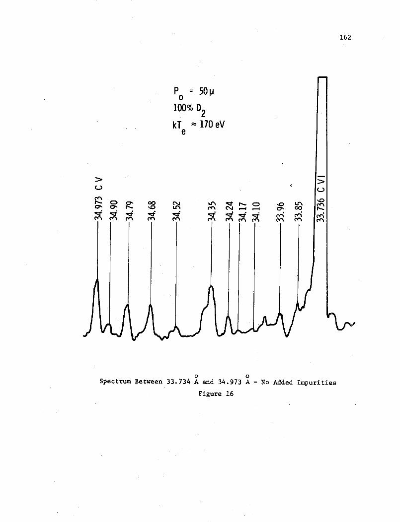
162
P 50 p0100% D2
kT ~ 170 eVe
oso o
0 0Spectrum Between 33.734 A and 34.973 A - No Added Impurities
Figure 16
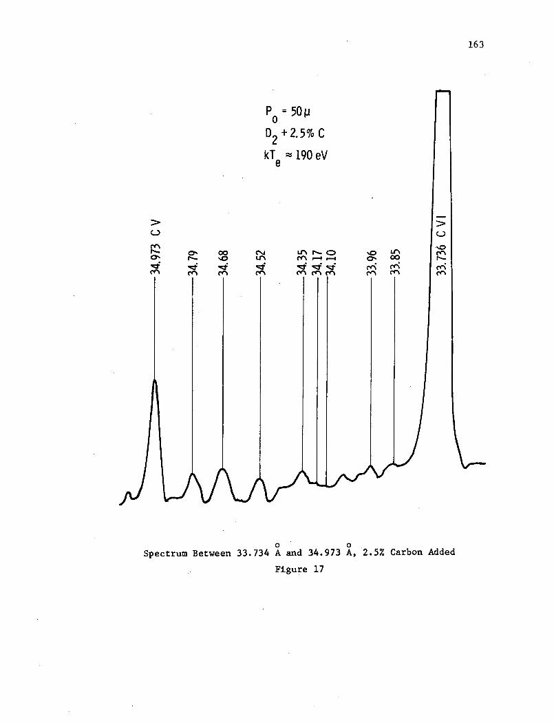
163
P 50Ip
D2 + 2.5% C
kTe - 190 eVe
00 C'.q:O un
-0: -ci
Lu-r - O .0 - r- yO 00
v .: a: cri ffiCrn Cn M Cn~7 M
0 0Spectrum Between 33.734 A and 34.973 A, 2.5% Carbon Added
Figure 17
cO
C,-O-
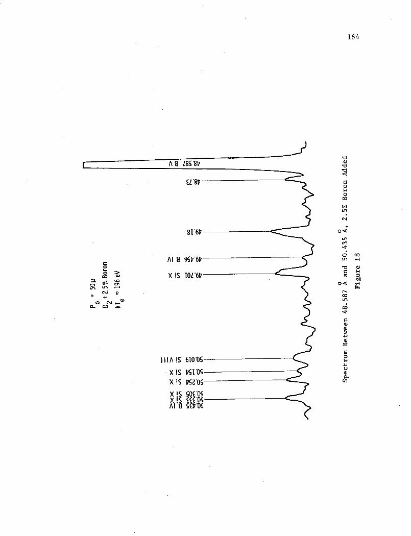
164
I AS L88V
0.- .
o N -.n C:
II
-V
81'62
AI 9 %'6z
X IS [OL'6 .
IA IS 610'05
X!S tI'Os-X !S KZ'OCX !S 50£'05 X !S t.°05 AlI 9 5E1;"0
0
U,o
Us
Qr
CO.
U,
U,3
co
0,)
r4rzd
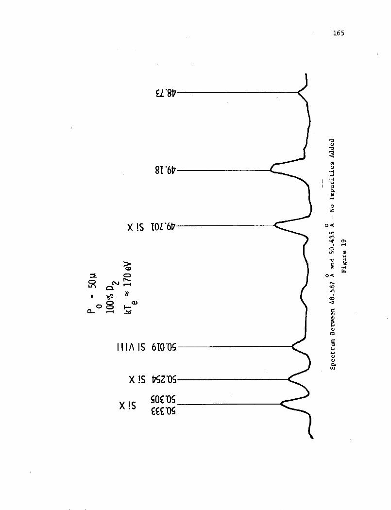
X !S IOL
ca
r-...
-'
08 -- .r
I I IA !S 610'05]
X !S tKZ'05
X !S
165
8L
81
M
Oh,-4
w04
O0.,4
4
IW
z
.4
0-4Co
U,
co-tt
C)o)0
1.rn
.4-:
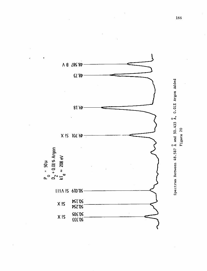
166
AS L85'82 -
'L 8'-
0
o
'-4
tI
X IS IOL'6V X
oX~~ c
o 0 )'
'v, mI-
YN lop1'5_
A i)
X !S o50c05
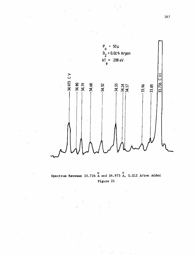
167
00
P = 50 p
D2 + 0.01% Argon
kT ~ 208eV e
U:S .1 as . £
fC % v ore% M M
0 0Spectrum Between 33.734 A and 34.973 A, 0.01% Arbon Added
Figure 21
0v
M.-
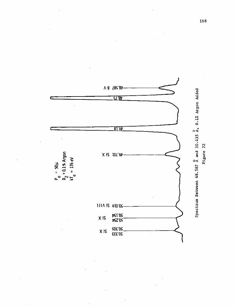
0 X !S IOL'6V-
'I +
X !S 'X a 50 05
168
04
"-4Q),
0
on-T
U-)
r-
0
Lfto
0U
w
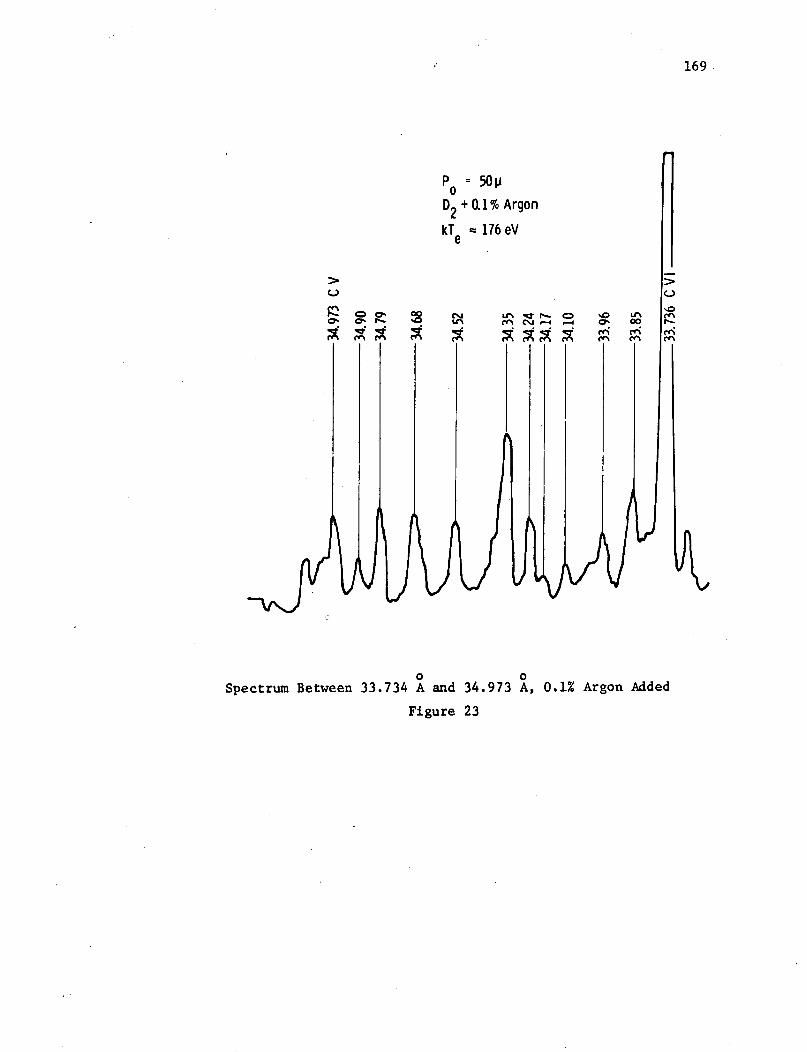
169
Po a 501P
D2 + 0.1% Argon
kTe = 176 eVe
U
a7. coI~- '0
0 0Spectrum Between 33.734 A and 34.973 A, 0.1% Argon Added
Figure 23
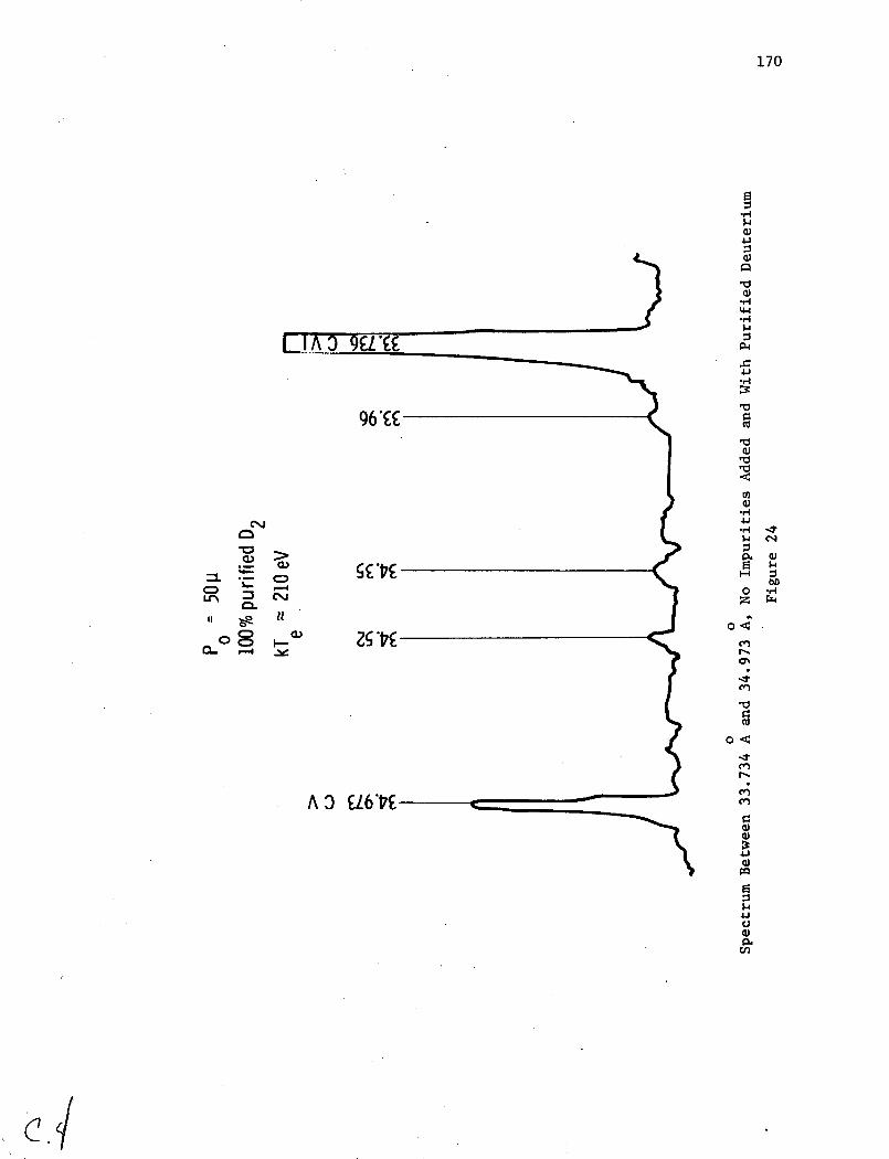
170
g$a
s-I
0G4
4a
P.-i
96C a-
'o _ o0xo g sa S~ 00. 4.1
AO 0M
U *a
oC
R3 ~~~~~~L6'PE~~~~~~
4.
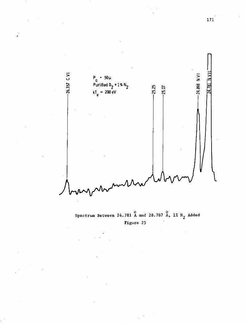
171
PO =50
,, Purified D +1% N2 ie, kT e 200 eV s
0 0Spectrum Between 24.781 A and 248.787 A, 1% N
2 Added
Figure 25
I
I
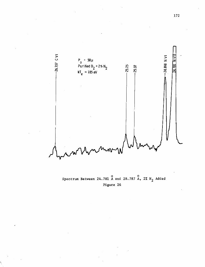
172
Po 50
Purified D2
+2% N2 i
kTe 185 eV
o oSpectrum Between 24.781 A and 28.787 A, 2% N2 Added
Figure 26
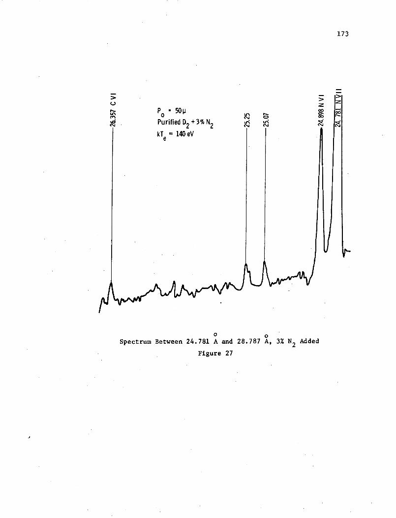
173
U
P = 50 1
Purified D2
+ 3% N2
kT = 140 eVe
0
Spectrum Between 24.781 A and 28.787
Figure 27
0A, 3% N
2Added
u. u-(.'J c..J
Recommended