
More Matrix Algebra; Mean Vectors and Covariance Matrices;
the Multivariate Normal Distribution
PSYC 943 (930): Fundamentals of Multivariate Modeling
Lecture 11: October 3, 2012
PSYC 943: Lecture 11

Today’s Class
• The conclusion of Friday’s lecture on matrix algebra Matrix inverse Zero/ones vector Matrix identity Matrix determinant NOTE: an introduction to principal components analysis will be relocated
later in the semester
• Putting matrix algebra to use in multivariate statistics
Mean vectors Covariance matrices
• The multivariate normal distribution
PSYC 943: Lecture 11 2
DATA EXAMPLE AND SAS
PSYC 943: Lecture 11 3

A Guiding Example
• To demonstrate matrix algebra, we will make use of data • Imagine that somehow I collected data SAT test scores for both the
Math (SATM) and Verbal (SATV) sections of 1,000 students
• The descriptive statistics of this data set are given below:
PSYC 943: Lecture 11 4
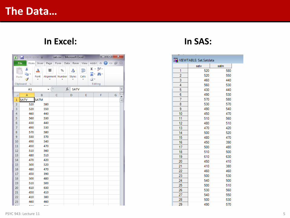
The Data…
In Excel: In SAS:
PSYC 943: Lecture 11 5
Matrix Computing: PROC IML
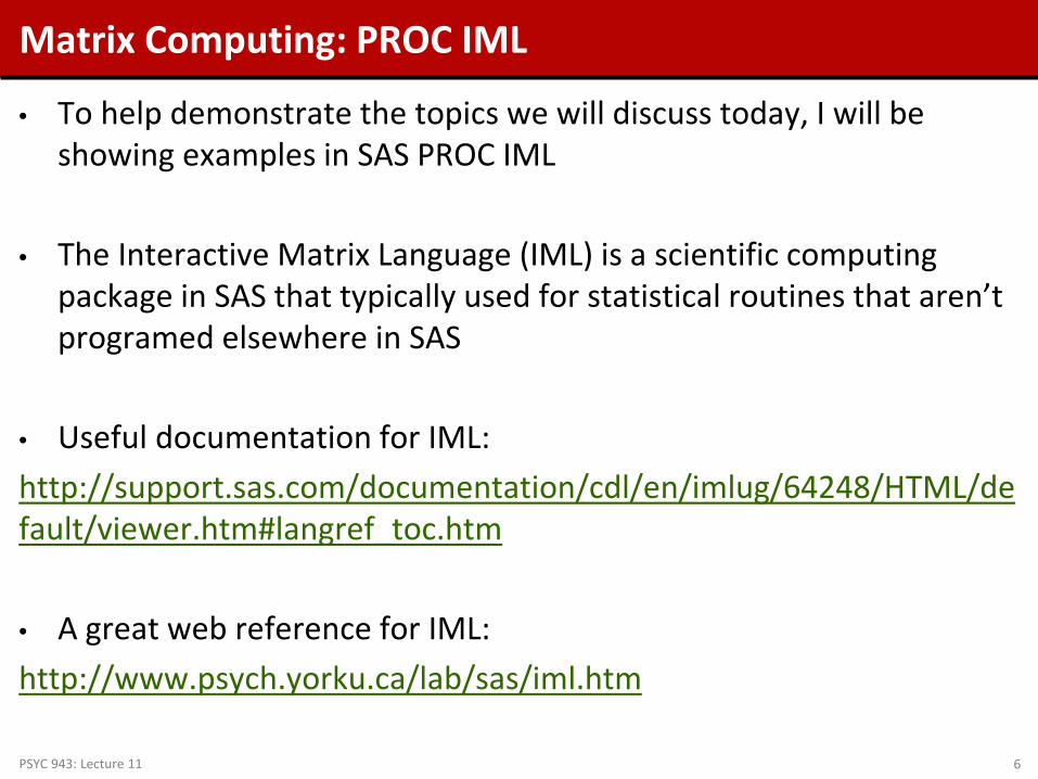
• To help demonstrate the topics we will discuss today, I will be showing examples in SAS PROC IML
• The Interactive Matrix Language (IML) is a scientific computing package in SAS that typically used for statistical routines that aren’t programed elsewhere in SAS
• Useful documentation for IML: http://support.sas.com/documentation/cdl/en/imlug/64248/HTML/default/viewer.htm#langref_toc.htm • A great web reference for IML: http://www.psych.yorku.ca/lab/sas/iml.htm
PSYC 943: Lecture 11 6

MATRIX ALGEBRA
PSYC 943: Lecture 11 7

Moving from Vectors to Matrices
• A matrix can be thought of as a collection of vectors Matrix operations are vector operations on steroids
• Matrix algebra defines a set of operations and entities on matrices I will present a version meant to mirror your previous algebra experiences
• Definitions: Identity matrix Zero vector Ones vector
• Basic Operations: Addition Subtraction Multiplication “Division”
PSYC 943: Lecture 11 8
Matrix Addition and Subtraction
• Matrix addition and subtraction are much like vector addition/subtraction
• Rules: Matrices must be the same size (rows and columns)
• Method:
The new matrix is constructed of element-by-element addition/subtraction of the previous matrices
• Order:
The order of the matrices (pre- and post-) does not matter
PSYC 943: Lecture 11 9

Matrix Addition/Subtraction
PSYC 943: Lecture 11 10
Matrix Multiplication
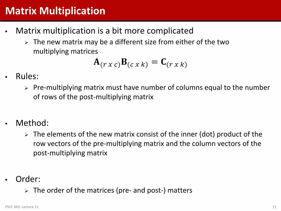
• Matrix multiplication is a bit more complicated The new matrix may be a different size from either of the two
multiplying matrices 𝐀(𝑟 𝑥 𝑐)𝐁(𝑐 𝑥 𝑘) = 𝐂(𝑟 𝑥 𝑘)
• Rules: Pre-multiplying matrix must have number of columns equal to the number
of rows of the post-multiplying matrix
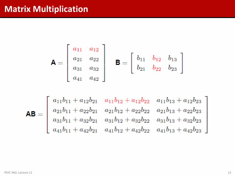
• Method:
The elements of the new matrix consist of the inner (dot) product of the row vectors of the pre-multiplying matrix and the column vectors of the post-multiplying matrix
• Order:
The order of the matrices (pre- and post-) matters
PSYC 943: Lecture 11 11
Matrix Multiplication
PSYC 943: Lecture 11 12
Multiplication in Statistics
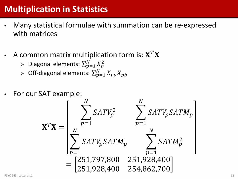
• Many statistical formulae with summation can be re-expressed with matrices
• A common matrix multiplication form is: 𝐗𝑇𝐗 Diagonal elements: ∑ 𝑋𝑝2𝑁
𝑝=1 Off-diagonal elements: ∑ 𝑋𝑝𝑎𝑋𝑝𝑏
𝑁𝑝=1
• For our SAT example:
𝐗𝑇𝐗 =
�𝑆𝑆𝑆𝑆𝑝2𝑁
𝑝=1
� 𝑆𝑆𝑆𝑆𝑝𝑆𝑆𝑆𝑆𝑝
𝑁
𝑝=1
� 𝑆𝑆𝑆𝑆𝑝𝑆𝑆𝑆𝑆𝑝
𝑁
𝑝=1
�𝑆𝑆𝑆𝑆𝑝2
𝑁
𝑝=1
= 251,797,800 251,928,400251,928,400 254,862,700
PSYC 943: Lecture 11 13
Identity Matrix
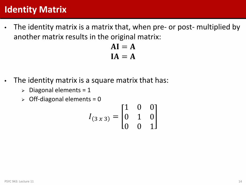
• The identity matrix is a matrix that, when pre- or post- multiplied by another matrix results in the original matrix:
𝐀𝐀 = 𝐀 𝐀𝐀 = 𝐀
• The identity matrix is a square matrix that has:
Diagonal elements = 1 Off-diagonal elements = 0
𝐼 3 𝑥 3 =1 0 00 1 00 0 1
PSYC 943: Lecture 11 14

Zero Vector
• The zero vector is a column vector of zeros
𝟎(3 𝑥 1) =000
• When pre- or post- multiplied the result is the zero vector: 𝐀𝟎 = 𝟎 𝟎𝐀 = 𝟎
PSYC 943: Lecture 11 15

Ones Vector
• A ones vector is a column vector of 1s:
𝟏(3 𝑥 1) =111
• The ones vector is useful for calculating statistical terms, such as the
mean vector and the covariance matrix
PSYC 943: Lecture 11 16

Matrix “Division”: The Inverse Matrix
• Division from algebra: First: 𝑎
𝑏= 1
𝑏𝑎 = 𝑏−1𝑎
Second: 𝑎𝑎
= 1
• “Division” in matrices serves a similar role For square and symmetric matrices, an inverse matrix is a matrix that when
pre- or post- multiplied with another matrix produces the identity matrix: 𝐀−1𝐀 = 𝐀 𝐀𝐀−𝟏 = 𝐀
• Calculation of the matrix inverse is complicated Even computers have a tough time
• Not all matrices can be inverted Non-invertible matrices are called singular matrices
In statistics, singular matrices are commonly caused by linear dependencies PSYC 943: Lecture 11 17
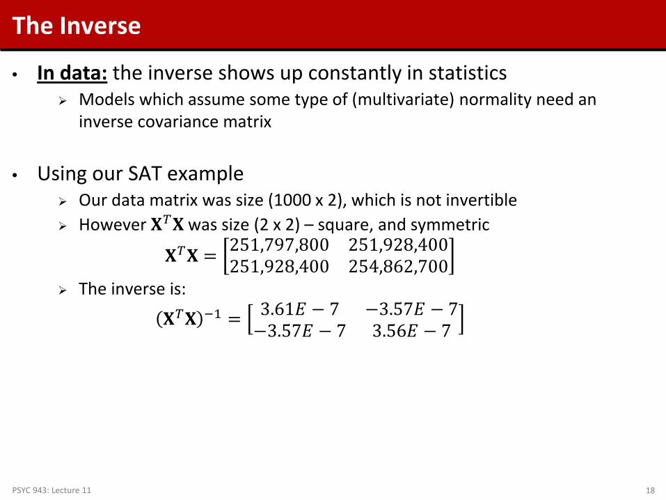
The Inverse
• In data: the inverse shows up constantly in statistics Models which assume some type of (multivariate) normality need an
inverse covariance matrix
• Using our SAT example Our data matrix was size (1000 x 2), which is not invertible However 𝐗𝑇𝐗 was size (2 x 2) – square, and symmetric
𝐗𝑇𝐗 = 251,797,800 251,928,400251,928,400 254,862,700
The inverse is:
𝐗𝑇𝐗 −1 = 3.61𝐸 − 7 −3.57𝐸 − 7−3.57𝐸 − 7 3.56𝐸 − 7
PSYC 943: Lecture 11 18
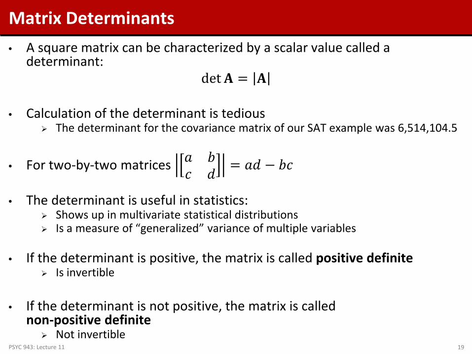
Matrix Determinants • A square matrix can be characterized by a scalar value called a
determinant: det𝐀 = 𝐀
• Calculation of the determinant is tedious
The determinant for the covariance matrix of our SAT example was 6,514,104.5
• For two-by-two matrices 𝑎 𝑏𝑐 𝑑 = 𝑎𝑑 − 𝑏𝑐
• The determinant is useful in statistics:
Shows up in multivariate statistical distributions Is a measure of “generalized” variance of multiple variables
• If the determinant is positive, the matrix is called positive definite
Is invertible
• If the determinant is not positive, the matrix is called non-positive definite
Not invertible PSYC 943: Lecture 11 19

Matrix Trace
• For a square matrix 𝐀 with V rows/columns, the trace is the sum of the diagonal elements:
𝑡𝑡𝐀 = �𝑎𝑣𝑣
𝑉
𝑣=1
• For our data, the trace of the correlation matrix is 2
For all correlation matrices, the trace is equal to the number of variables because all diagonal elements are 1
• The trace is considered the total variance in multivariate statistics
Used as a target to recover when applying statistical models
PSYC 943: Lecture 11 20

Matrix Algebra Operations (for help in reading stats manuals)
• 𝐀 + 𝐁 + 𝐂 = 𝐀 + (𝐁 + 𝐂)
• 𝐀 + 𝐁 = 𝐁 + 𝐀 • 𝑐 𝐀 + 𝐁 = 𝑐𝐀 + 𝑐𝐁 • 𝑐 + 𝑑 𝐀 = 𝑐𝐀 + 𝑑𝐀 • 𝐀 + 𝐁 𝑇 = 𝐀𝑇 + 𝐁𝑇 • 𝑐𝑑 𝐀 = 𝑐(𝑑𝐀) • 𝑐𝐀 𝑇 = 𝑐𝐀𝑇 • 𝑐 𝐀𝐁 = 𝑐𝐀 𝐁 • 𝐀 𝐁𝐂 = 𝐀𝐁 𝐂
• 𝐀 𝐁 + 𝐂 = 𝐀𝐁 + 𝐀𝐂 • 𝐀𝐁 𝑇 = 𝐁𝑇𝐀𝑇 • For 𝑥𝑗 such that 𝑆𝑥𝑗 exists:
�𝐀𝐱𝑗 =𝑁
𝑗=1
𝐀�𝐱𝑗
𝑁
𝑗=1
� 𝐀𝐱𝑗 𝐀𝐱𝑗𝑇 =
𝑁
𝑗=1
𝐀 �𝐱𝑗𝐱𝑗𝑇𝑁
𝑗=1
𝐀𝑇
PSYC 943: Lecture 11 21
MULTIVARIATE STATISTICS AND DISTRIBUTIONS
PSYC 943: Lecture 11 22

Multivariate Statistics • Up to this point in this course, we have focused on the prediction (or
modeling) of a single variable Conditional distributions (aka, generalized linear models)
• Multivariate statistics is about exploring joint distributions
How variables relate to each other simultaneously
• Therefore, we must adapt our conditional distributions to have multiple variables, simultaneously (later, as multiple outcomes)
• We will now look at the joint distributions of two variables 𝑓 𝑥1, 𝑥2 or in matrix form: 𝑓 𝐗 (where 𝐗 is size N x 2; 𝑓 𝐗 gives a scalar/single number)
Beginning with two, then moving to anything more than two We will begin by looking at multivariate descriptive statistics
Mean vectors and covariance matrices
• Today, we will only consider the joint distribution of sets of variables – but next time we will put this into a GLM-like setup
The joint distribution will the be conditional on other variables PSYC 943: Lecture 11 23
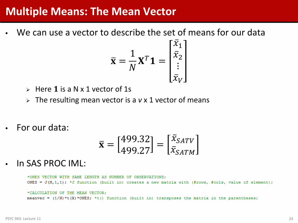
Multiple Means: The Mean Vector
• We can use a vector to describe the set of means for our data
𝐱� =1𝑁𝐗𝑇𝟏 =
�̅�1�̅�2⋮�̅�𝑉
Here 𝟏 is a N x 1 vector of 1s The resulting mean vector is a v x 1 vector of means
• For our data:
𝐱� = 499.32499.27 = �̅�𝑆𝑆𝑇𝑉
�̅�𝑆𝑆𝑇𝑆
• In SAS PROC IML:
PSYC 943: Lecture 11 24

Mean Vector: Graphically
• The mean vector is the center of the distribution of both variables
PSYC 943: Lecture 11 25
200
400
600
800
200 400 600 800
SATV
SATM

Covariance of a Pair of Variables
• The covariance is a measure of the relatedness Expressed in the product of the units of the two variables:
𝑠𝑥1𝑥2 =1𝑁� 𝑥𝑝1 − �̅�1 𝑥𝑝2 − �̅�2
𝑁
𝑝=1
The covariance between SATV and SATM was 3,132.22 (in SAT Verbal-Maths)
The denominator N is the ML version – unbiased is N-1
• Because the units of the covariance are difficult to understand, we more commonly describe association (correlation) between two variables with correlation Covariance divided by the product of each variable’s standard deviation
PSYC 943: Lecture 11 26

Correlation of a Pair of Varibles
• Correlation is covariance divided by the product of the standard deviation of each variable:
𝑡𝑥1𝑥2 =𝑠𝑥1𝑥2
𝑠𝑥12 𝑠𝑥2
2
The correlation between SATM and SATV was 0.78
• Correlation is unitless – it only ranges between -1 and 1
If 𝑥1 and 𝑥2 both had variances of 1, the covariance between them would be a correlation Covariance of standardized variables = correlation
PSYC 943: Lecture 11 27
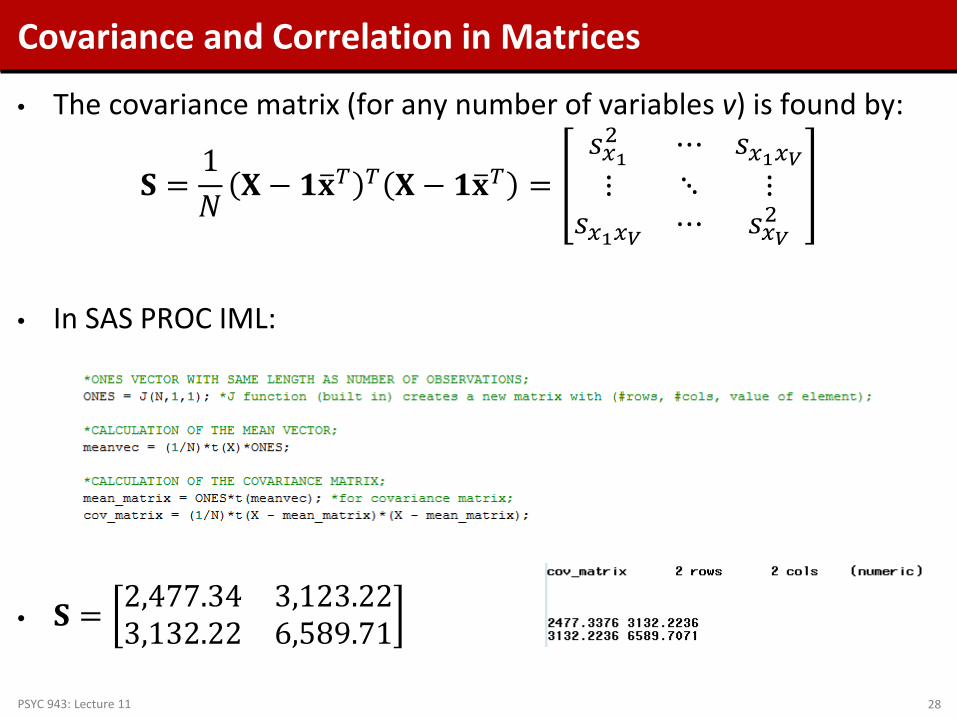
Covariance and Correlation in Matrices
• The covariance matrix (for any number of variables v) is found by:
𝐒 =1𝑁
𝐗 − 𝟏𝐱�𝑇 𝑇 𝐗 − 𝟏𝐱�𝑇 =𝑠𝑥12 ⋯ 𝑠𝑥1𝑥𝑉⋮ ⋱ ⋮
𝑠𝑥1𝑥𝑉 ⋯ 𝑠𝑥𝑉2
• In SAS PROC IML:
• 𝐒 = 2,477.34 3,123.223,132.22 6,589.71
PSYC 943: Lecture 11 28
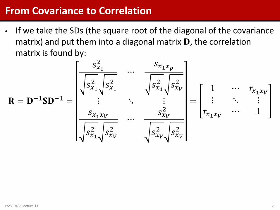
From Covariance to Correlation
• If we take the SDs (the square root of the diagonal of the covariance matrix) and put them into a diagonal matrix 𝐃, the correlation matrix is found by:
𝐑 = 𝐃−1𝐒𝐃−1 =
𝑠𝑥12
𝑠𝑥12 𝑠𝑥1
2⋯
𝑠𝑥1𝑥𝑝
𝑠𝑥12 𝑠𝑥𝑉
2
⋮ ⋱ ⋮𝑠𝑥1𝑥𝑉
𝑠𝑥12 𝑠𝑥𝑉
2⋯
𝑠𝑥𝑉2
𝑠𝑥𝑉2 𝑠𝑥𝑉
2
=1 ⋯ 𝑡𝑥1𝑥𝑉⋮ ⋱ ⋮
𝑡𝑥1𝑥𝑉 ⋯ 1
PSYC 943: Lecture 11 29
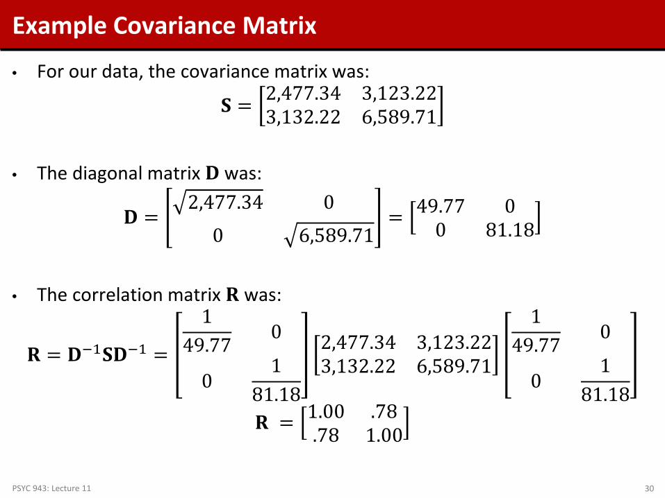
Example Covariance Matrix
• For our data, the covariance matrix was:
𝐒 = 2,477.34 3,123.223,132.22 6,589.71
• The diagonal matrix 𝐃 was:
𝐃 =2,477.34 0
0 6,589.71= 49.77 0
0 81.18
• The correlation matrix 𝐑 was:
𝐑 = 𝐃−1𝐒𝐃−1 =
149.77 0
01
81.18
2,477.34 3,123.223,132.22 6,589.71
149.77 0
01
81.18
𝐑 = 1.00 .78.78 1.00
PSYC 943: Lecture 11 30
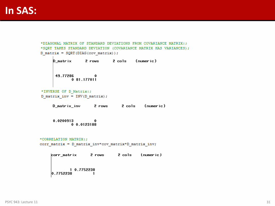
In SAS:
PSYC 943: Lecture 11 31
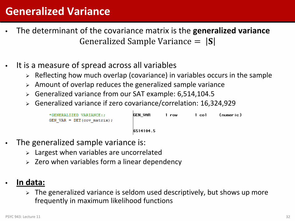
Generalized Variance • The determinant of the covariance matrix is the generalized variance
Generalized Sample Variance = 𝐒
• It is a measure of spread across all variables Reflecting how much overlap (covariance) in variables occurs in the sample Amount of overlap reduces the generalized sample variance Generalized variance from our SAT example: 6,514,104.5 Generalized variance if zero covariance/correlation: 16,324,929
• The generalized sample variance is: Largest when variables are uncorrelated Zero when variables form a linear dependency
• In data:
The generalized variance is seldom used descriptively, but shows up more frequently in maximum likelihood functions
PSYC 943: Lecture 11 32
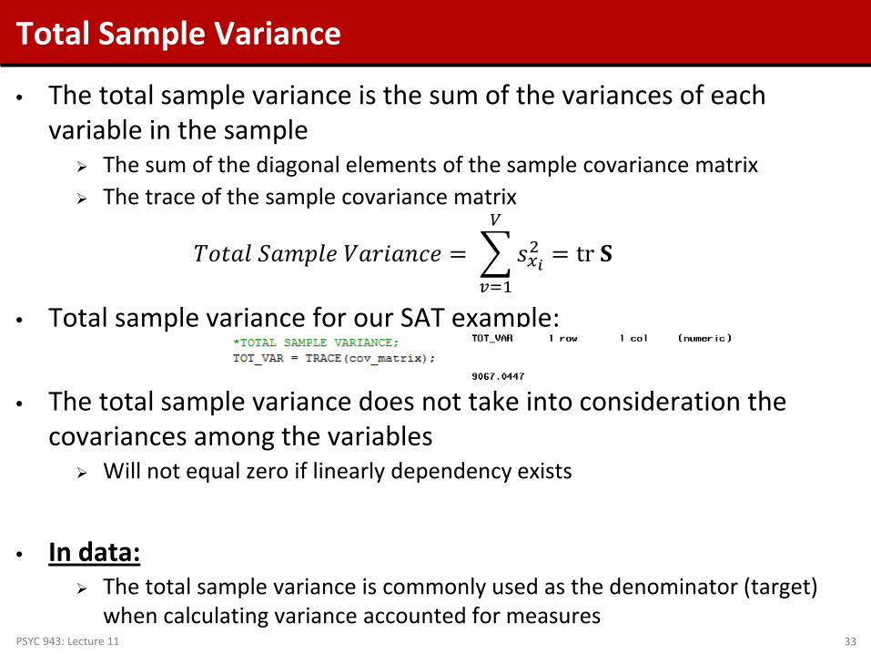
Total Sample Variance
• The total sample variance is the sum of the variances of each variable in the sample The sum of the diagonal elements of the sample covariance matrix The trace of the sample covariance matrix
𝑆𝑇𝑡𝑎𝑇 𝑆𝑎𝑆𝑆𝑇𝑆 𝑆𝑎𝑡𝑉𝑎𝑉𝑐𝑆 = �𝑠𝑥𝑖2
𝑉
𝑣=1
= tr 𝐒
• Total sample variance for our SAT example:
• The total sample variance does not take into consideration the covariances among the variables Will not equal zero if linearly dependency exists
• In data:
The total sample variance is commonly used as the denominator (target) when calculating variance accounted for measures
PSYC 943: Lecture 11 33

MULTIVARIATE DISTRIBUTIONS (VARIABLES ≥ 2)
PSYC 943: Lecture 11 34

Multivariate Normal Distribution
• The multivariate normal distribution is the generalization of the univariate normal distribution to multiple variables The bivariate normal distribution just shown is part of the MVN
• The MVN provides the relative likelihood of observing all V variables
for a subject p simultaneously: 𝐱𝑝 = 𝑥𝑝1 𝑥𝑝2 … 𝑥𝑝𝑉
• The multivariate normal density function is:
𝑓 𝐱𝑝 =1
2𝜋𝑉2 𝚺
12
exp −𝐱𝑝𝑇 − 𝝁 𝑇𝚺−1 𝐱𝑝𝑇 − 𝝁
2
PSYC 943: Lecture 11 35

The Multivariate Normal Distribution
𝑓 𝐱𝑝 =1
2𝜋𝑉2 𝚺
12
exp −𝐱𝑝𝑇 − 𝝁 𝑇𝚺−1 𝐱𝑝𝑇 − 𝝁
2
• The mean vector is 𝝁 =
𝜇𝑥1𝜇𝑥2⋮𝜇𝑥𝑉
• The covariance matrix is 𝚺 =
𝜎𝑥12 𝜎𝑥1𝑥2 ⋯ 𝜎𝑥1𝑥𝑉
𝜎𝑥1𝑥2 𝜎𝑥22 ⋯ 𝜎𝑥2𝑥𝑉
⋮ ⋮ ⋱ ⋮𝜎𝑥1𝑥𝑉 𝜎𝑥2𝑥𝑉 ⋯ 𝜎𝑥𝑉
2
The covariance matrix must be non-singular (invertible)
PSYC 943: Lecture 11 36

Comparing Univariate and Multivariate Normal Distributions
• The univariate normal distribution:
𝑓 𝑥𝑝 =12𝜋𝜎2
exp −𝑥 − 𝜇 2
2𝜎2
• The univariate normal, rewritten with a little algebra:
𝑓 𝑥𝑝 =1
2𝜋12|𝜎2|
12
exp −𝑥 − 𝜇 𝜎−
12 𝑥 − 𝜇
2
• The multivariate normal distribution
𝑓 𝐱𝑝 =1
2𝜋𝑉2 𝚺
12
exp −𝐱𝑝𝑇 − 𝝁 𝑇𝚺−1 𝐱𝑝𝑇 − 𝝁
2
When 𝑆 = 1 (one variable), the MVN is a univariate normal distribution
PSYC 943: Lecture 11 37
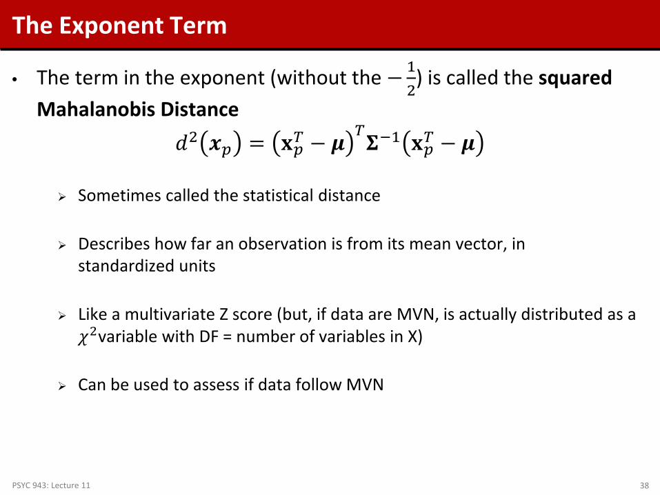
The Exponent Term
• The term in the exponent (without the −12) is called the squared
Mahalanobis Distance 𝑑2 𝒙𝑝 = 𝐱𝑝𝑇 − 𝝁 𝑇𝚺−1 𝐱𝑝𝑇 − 𝝁
Sometimes called the statistical distance
Describes how far an observation is from its mean vector, in
standardized units
Like a multivariate Z score (but, if data are MVN, is actually distributed as a 𝜒2variable with DF = number of variables in X)
Can be used to assess if data follow MVN
PSYC 943: Lecture 11 38

Multivariate Normal Notation
• Standard notation for the multivariate normal distribution of v variables is 𝑁𝑣 𝝁,𝚺 Our SAT example would use a bivariate normal: 𝑁2 𝝁,𝚺
• In data: The multivariate normal distribution serves as the basis for most every
statistical technique commonly used in the social and educational sciences General linear models (ANOVA, regression, MANOVA) General linear mixed models (HLM/multilevel models) Factor and structural equation models (EFA, CFA, SEM, path models) Multiple imputation for missing data
Simply put, the world of commonly used statistics revolves around the
multivariate normal distribution Understanding it is the key to understanding many statistical methods
PSYC 943: Lecture 11 39
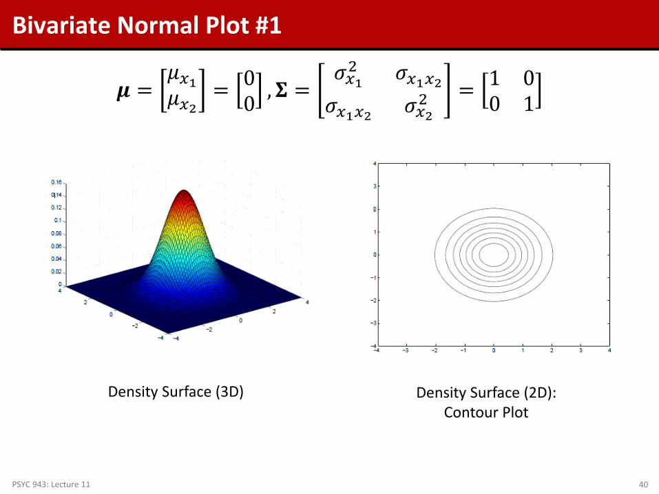
Bivariate Normal Plot #1
𝝁 =𝜇𝑥1𝜇𝑥2
= 00 ,𝚺 =
𝜎𝑥12 𝜎𝑥1𝑥2
𝜎𝑥1𝑥2 𝜎𝑥22 = 1 0
0 1
Density Surface (3D) Density Surface (2D): Contour Plot
PSYC 943: Lecture 11 40

Bivariate Normal Plot #2 (Multivariate Normal)
𝝁 =𝜇𝑥1𝜇𝑥2
= 00 ,𝚺 =
𝜎𝑥12 𝜎𝑥1𝑥2
𝜎𝑥1𝑥2 𝜎𝑥22 = 1 .5
.5 1
Density Surface (3D) Density Surface (2D): Contour Plot
PSYC 943: Lecture 11 41

Multivariate Normal Properties
• The multivariate normal distribution has some useful properties that show up in statistical methods
• If 𝐗 is distributed multivariate normally: 1. Linear combinations of 𝐗 are normally distributed
2. All subsets of 𝐗 are multivariate normally distributed
3. A zero covariance between a pair of variables of 𝐗 implies that the
variables are independent
4. Conditional distributions of 𝐗 are multivariate normal
PSYC 943: Lecture 11 42

Multivariate Normal Distribution in PROC IML
• To demonstrate how the MVN works, we will now investigate how the PDF provides the likelihood (height) for a given observation: Here we will use the SAT data and assume the sample mean vector and
covariance matrix are known to be the true:
𝝁 = 499.32498.27 ; 𝐒 = 2,477.34 3,123.22
3,132.22 6,589.71
• We will compute the likelihood value for several observations (SEE EXAMPLE SAS SYNTAX FOR HOW THIS WORKS): 𝒙631,⋅ = 590 730 ; 𝑓 𝒙 = 0.00000087528 𝒙717,⋅ = 340 300 ; 𝑓 𝒙 = 0.00000037082 𝒙 = 𝒙� = 499.32 498.27 ; 𝑓 𝒙 = 0.0000624
• Note: this is the height for these observations, not the joint likelihood across all the data Next time we will use PROC MIXED to find the parameters in 𝝁 and 𝚺 using
maximum likelihood
PSYC 943: Lecture 11 43

Likelihoods…From SAS
PSYC 943: Lecture 11 44
𝑓 𝐱𝑝 =1
2𝜋𝑣2 𝚺
12
exp −𝐱𝑝𝑇 − 𝝁 𝑇𝚺−1 𝐱𝑝𝑇 − 𝝁
2
Wrapping Up
• The last two classes set the stage to discuss multivariate statistical methods that use maximum likelihood
• Matrix algebra was necessary so as to concisely talk about our distributions (which will soon be models)
• The multivariate normal distribution will be necessary to understand as it is the most commonly used distribution for estimation of multivariate models
• Friday we will get back into data analysis – but for multivariate observations…using SAS PROC MIXED Each term of the MVN will be mapped onto the PROC MIXED output
PSYC 943: Lecture 11 45
Recommended


