Multivariate Resolution in Chemistry
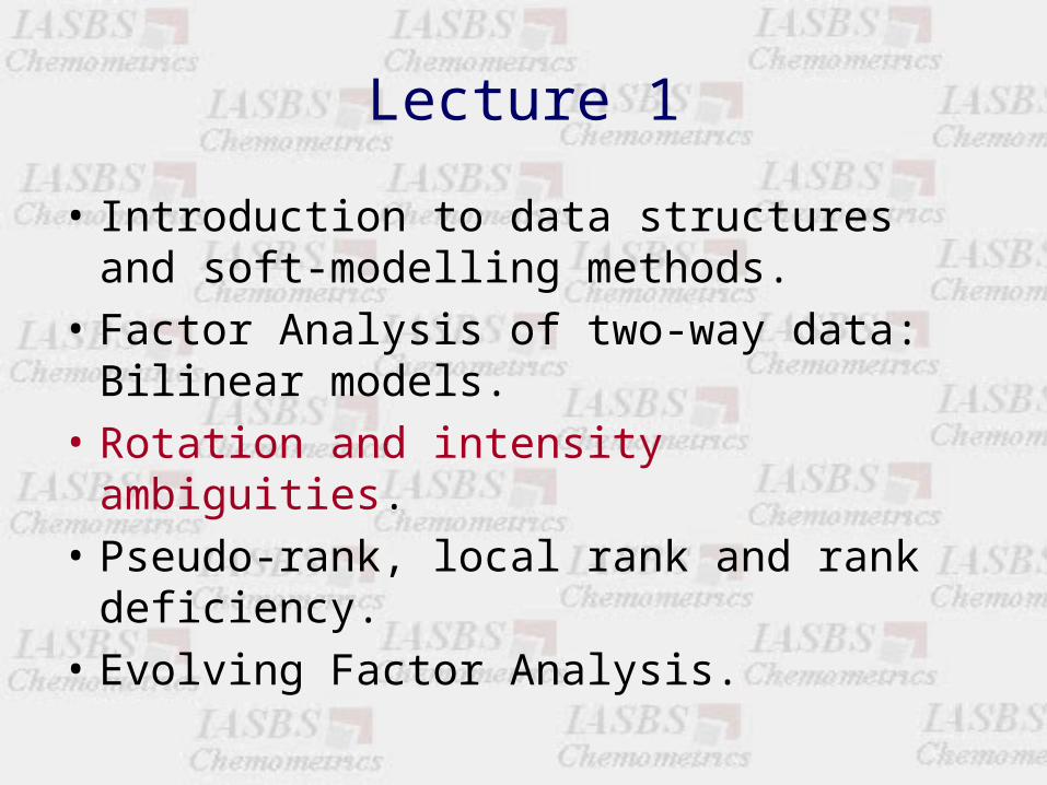
Lecture 1
Roma TaulerRoma TaulerIIQAB-CSIC, Spain
e-mail: [email protected]
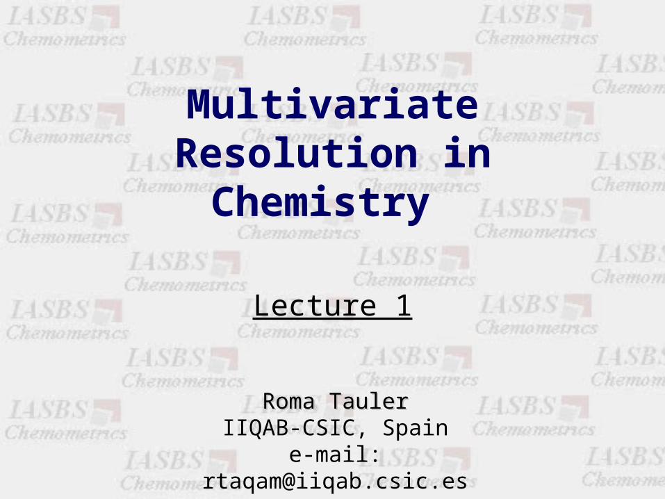
Lecture 1
• Introduction to data structures and soft-modelling methods.
• Factor Analysis of two-way data: Bilinear models.
• Rotation and intensity ambiguities.
• Pseudo-rank, local rank and rank deficiency.
• Evolving Factor Analysis.
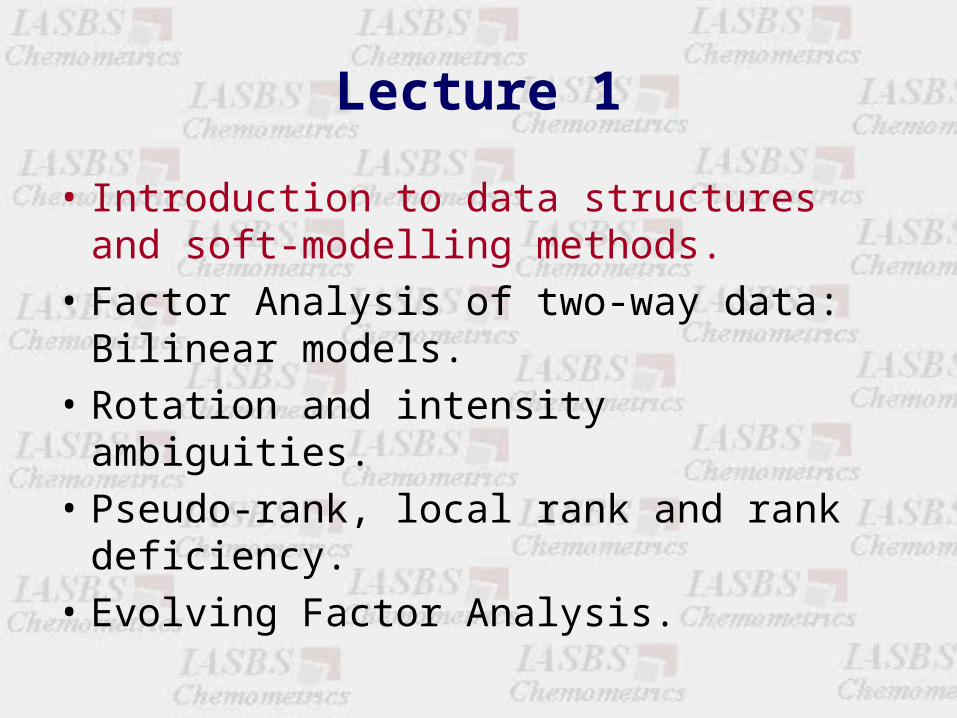
Chemical sensors and analytical data structures
one variable x1 e.g. pH
two variables x1,x2 e.g pH i T
three variables x1, x2 and x3
e.g. pH, T i P
n variables ?????
* ***** * ** *** *
pH
T
pH
pH
T
P
*
***
**
*
*
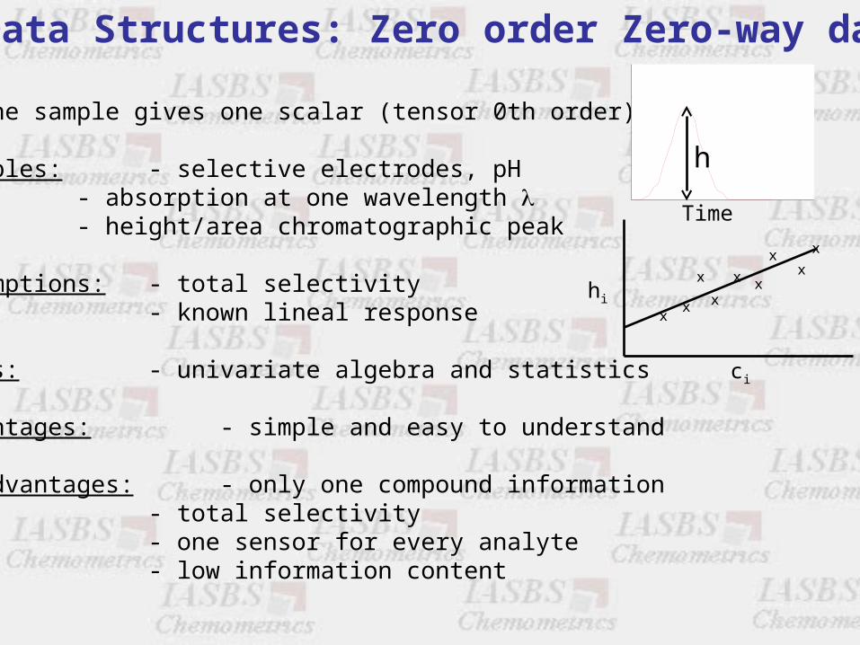
x; one sample gives one scalar (tensor 0th order)
Examples: - selective electrodes, pH- absorption at one wavelength - height/area chromatographic peak
Assumptions: - total selectivity- known lineal response
Tools: - univariate algebra and statistics
Advantages: - simple and easy to understand
Disadvantages: - only one compound information- total selectivity
- one sensor for every analyte- low information content
c
h
Time
xx
x
x
x x
xx
x
ci
hi
Data Structures: Zero order Zero-way data
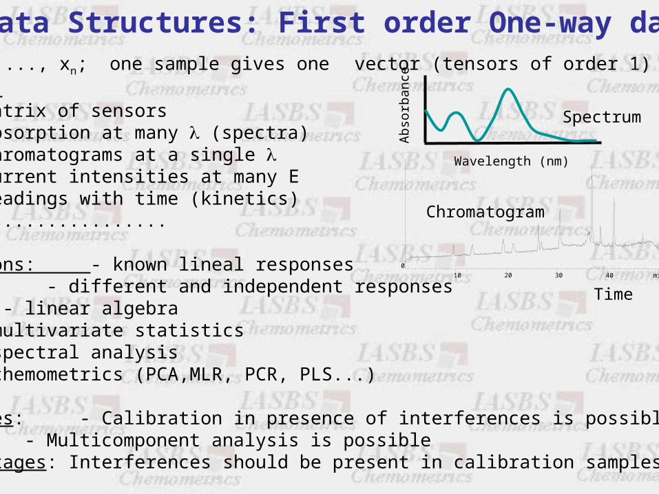
x1, x2, ....., xn; one sample gives one vector (tensors of order 1)Examples:
- matrix of sensors- absorption at many (spectra)- chromatograms at a single - current intensities at many E- readings with time (kinetics)-..................
Assumptions: - known lineal responses - different and independent responses
Tools: - linear algebra - multivariate statistics - spectral analysis - chemometrics (PCA,MLR, PCR, PLS...)
Advantages: - Calibration in presence of interferences is possible - Multicomponent analysis is possible
Disadvantages: Interferences should be present in calibration samples
Spectrum
Wavelength (nm)
Abso
rban
ce
min10 20 30 40
0
Time
Chromatogram
Data Structures: First order One-way data
xij; each sample gives a datatable/matrix; tensor of order 2X = xkyk
T
Examples: - LC-DAD; LC-FTIR; GC-MS; LC-MS; FIA-DAD; CE-MS,.. (hyphenated techniques)- esp. excitation/emission (fluorescence)- MS/MS, NMR 2D, GCxGC-MS ...- spectroscopic/voltammetric monitoring of chemical reactions/processes with pH, time, T, etc.
Assumptions: - linear responses- sufficient rank (of the data matrices)
Tools: - linear algebra- chemometrics
Advantages: - calibration for the analyte in the presence of interferences not modelled in calibration samples is possible- full characterization of the analyte and interferents may be possible- few calibration samples are needed (only one sample calibration)
Wavelengths
Elu
tio
nti
me
s Spectrum
Ch
rom
ato
gra
m
Wavelengths
Elu
tio
nti
me
s Spectrum
Ch
rom
ato
gra
m
Data Structures: Second order / Two-way data
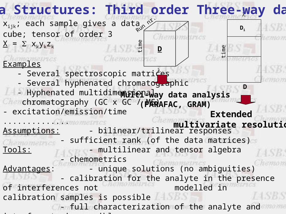
xijk; each sample gives a datacube; tensor of order 3X = xkykzk
Examples- Several spectroscopic matrices- Several hyphenated chromatographic- Hyphenated multidimensional chromatography (GC x GC / MS)
- excitation/emission/time..............Assumptions: - bilinear/trilinear responses
- sufficient rank (of the data matrices)Tools: - multilinear and tensor algebra
- chemometricsAdvantages: - unique solutions (no ambiguities)
- calibration for the analyte in the presence of interferences not modelled in calibration samples is possible
- full characterization of the analyte and interferents is possible- few calibration samples are needed (only one sample calibration)
Dtime
Run nr.
D
Di
time
Multi-way data analysis(PARAFAC, GRAM)
Extended multivariate resolution
Data Structures: Third order Three-way data
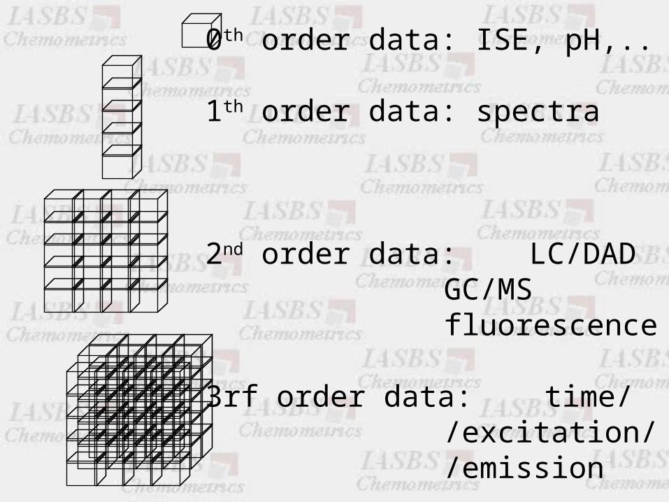
0th order data: ISE, pH,..
1th order data: spectra
2nd order data: LC/DAD GC/MS fluorescence
3rf order data: time/ /excitation/ /emission
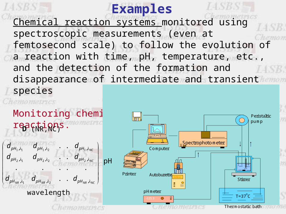
ExamplesChemical reaction systems monitored using spectroscopic measurements (even at femtosecond scale) to follow the evolution of a reaction with time, pH, temperature, etc., and the detection of the formation and disappearance of intermediate and transient species
Monitoring chemical reactions.
T=37oC
Spectrophotometer
Peristalticpump
0.050 ml
-125.3
pHmeter
Autoburette
Computer
PrinterStirrer
Thermostatic bath
D (NR,NC)
NCNRNRNR
NC
NC
pHpHpH
pHpHpH
pHpHpH
ddd
ddd
ddd
,,,
,,,
,,,
..
.....
..
..
21
22212
12111
pH
wavelength
Examples
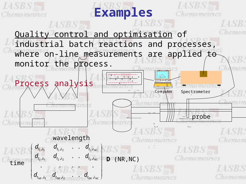
Quality control and optimisation of industrial batch reactions and processes, where on-line measurements are applied to monitor the process.
Process analysis
Computer Spectrometer
*
*
*
* ***
*
*
* *
probe
D (NR,NC)
NCNRNRNR
NC
NC
ttt
ttt
ttt
ddd
ddd
ddd
,,,
,,,
,,,
..
.....
..
..
21
22212
12111
time
wavelength
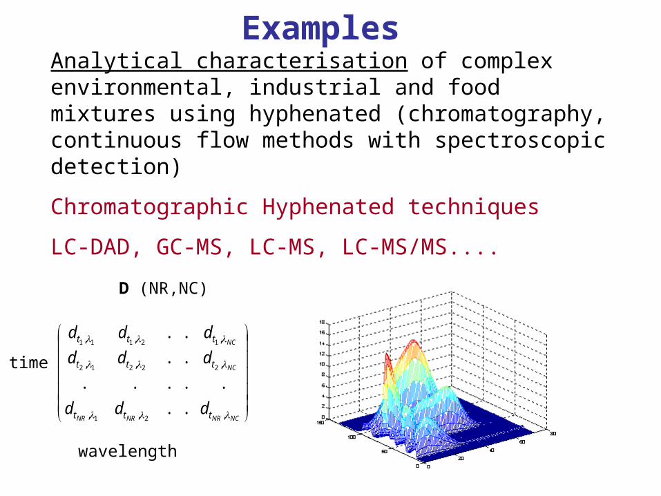
Examples Analytical characterisation of complex environmental, industrial and food mixtures using hyphenated (chromatography, continuous flow methods with spectroscopic detection)
Chromatographic Hyphenated techniques
LC-DAD, GC-MS, LC-MS, LC-MS/MS....
D (NR,NC)
NCNRNRNR
NC
NC
ttt
ttt
ttt
ddd
ddd
ddd
,,,
,,,
,,,
..
.....
..
..
21
22212
12111
time
wavelength
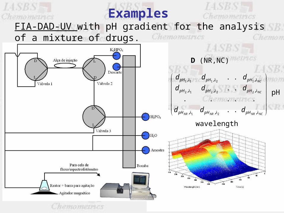
Examples FIA-DAD-UV with pH gradient for the analysis of a mixture of drugs.
D (NR,NC)
NCNRNRNR
NC
NC
pHpHpH
pHpHpH
pHpHpH
ddd
ddd
ddd
,,,
,,,
,,,
..
.....
..
..
21
22212
12111
pH
wavelength
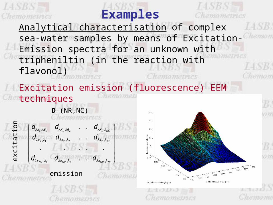
Examples Analytical characterisation of complex sea-water samples by means of Excitation-Emission spectra for an unknown with tripheniltin (in the reaction with flavonol)
Excitation emission (fluorescence) EEM techniques
NCNRNRNR
NC
NC
xxx
xxx
xexex
ddd
ddd
ddd
,,,
,,,
,,,
..
.....
..
..
21
22212
12111
D (NR,NC)
emission
exci
tatio
n
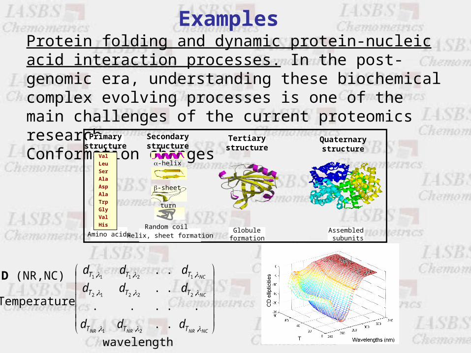
Examples Protein folding and dynamic protein-nucleic acid interaction processes. In the post-genomic era, understanding these biochemical complex evolving processes is one of the main challenges of the current proteomics research.Conformation changes
D (NR,NC)
NCNRNRNR
NC
NC
TTT
TTT
TTT
ddd
ddd
ddd
,,,
,,,
,,,
..
.....
..
..
21
22212
12111
Temperature
wavelength
Primarystructure
Secondarystructure
Tertiarystructure
Amino acidsGlobule
formationAssembled subunitsHelix, sheet formation
Val
Leu
Ser
Ala
Asp
Ala
Trp
Gly
Val
His
-helix
-sheet
turn
Random coil
Quaternarystructure
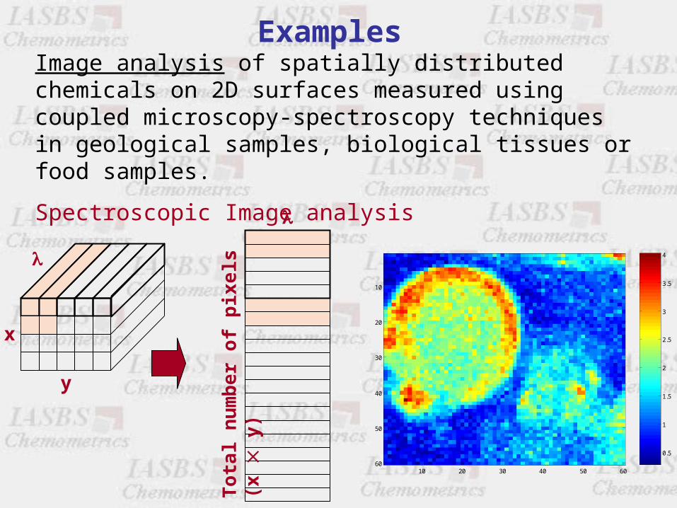
Examples Image analysis of spatially distributed chemicals on 2D surfaces measured using coupled microscopy-spectroscopy techniques in geological samples, biological tissues or food samples.
Spectroscopic Image analysis
0.5
1
1.5
2
2.5
3
3.5
4
10 20 30 40 50 60
10
20
30
40
50
60
x
y
T
ota
l nu
mb
er o
f p
ixe
ls (
x
y)
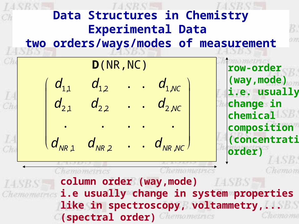
Data Structures in ChemistryExperimental Data
two orders/ways/modes of measurement
d d d
d d d
d d d
NC
NC
NR NR NR NC
1 1 1 2 1
2 1 2 2 2
1 2
, , ,
, , ,
, , ,
. .
. .
. . . . .
. .
row-order(way,mode)i.e. usuallychange in chemical composition (concentrationorder)
column order (way,mode)i.e usually change in system propertieslike in spectroscopy, voltammetry,...(spectral order)
D(NR,NC)
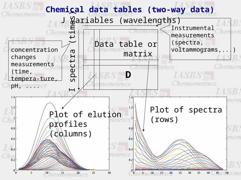
Chemical data tables (two-way data)
I sp
ectr
a (t
imes
)
J variables (wavelengths)
Data table or matrix
D
Instrumental measurements(spectra,voltammograms,...)concentration
changesmeasurements(time, tempera-ture, pH, ....
0 5 10 15 20 25 300
0.2
0.4
0.6
0.8
1
1.2
1.4
0 5 10 15 20 25 30 35 40 45 500
0.2
0.4
0.6
0.8
1
1.2
1.4
Plot of spectra(rows)
Plot of elutionprofiles (columns)
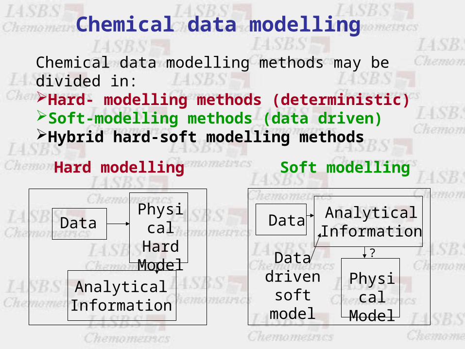
Chemical data modelling methods may be divided in:Hard- modelling methods (deterministic)Soft-modelling methods (data driven)Hybrid hard-soft modelling methods
Chemical data modelling
Soft modellingHard modelling
DataPhysical
HardModel
AnalyticalInformation
Data AnalyticalInformation
PhysicalModel
Datadriven
softmodel
?
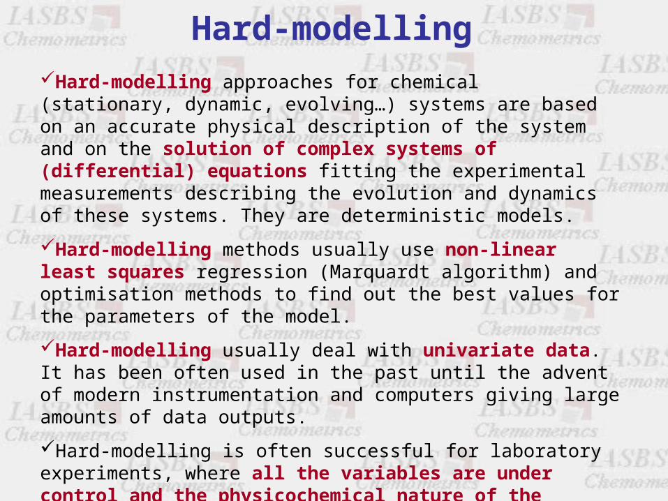
Hard-modelling approaches for chemical (stationary, dynamic, evolving…) systems are based on an accurate physical description of the system and on the solution of complex systems of (differential) equations fitting the experimental measurements describing the evolution and dynamics of these systems. They are deterministic models.
Hard-modelling methods usually use non-linear least squares regression (Marquardt algorithm) and optimisation methods to find out the best values for the parameters of the model.
Hard-modelling usually deal with univariate data. It has been often used in the past until the advent of modern instrumentation and computers giving large amounts of data outputs.
Hard-modelling is often successful for laboratory experiments, where all the variables are under control and the physicochemical nature of the dynamic model is known and can be fully described using a known mathematical model
Hard-modelling
However, and even at a laboratory level, there are examples where hard-modelling requirements and constraints are not totally fulfilled or no physicochemical model is known to describe the process (e.g. in chromatographic separations or in protein folding experiments).
Data sets obtained from the study of natural and industrial evolving processes are too complex and difficult to analyse using hard-modelling methods. In these cases, there is no known physical model available or it is too complex to be set in a general way.
Advanced hard-modelling in industrial applications has been attempted to model experimental difficulties, such as changes in temperature, pH, ionic strength and activity coefficients. This is a very difficult task!
Hard-modelling
Data Fitting in the Chemical SciencesP. Gans, John Wiley and Sons, New York 1992
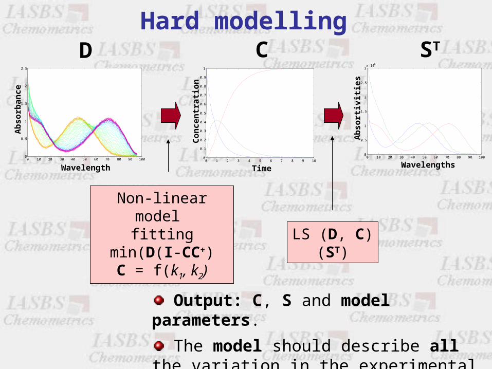
0 10 20 30 40 50 60 70 80 90 1000
0.5
1
1.5
2
2.5
3x 10⁴
Wavelengths
Ab
so
rtiv
itie
s
LS (D, C)(ST)
ST
0 10 20 30 40 50 60 70 80 90 1000
0.5
1
1.5
2
2.5
Wavelength
Ab
so
rba
nc
e
0 1 2 3 4 5 6 7 8 9 100
0.1
0.2
0.3
0.4
0.5
0.6
0.7
0.8
0.9
1
Time
Co
nc
en
tra
tio
nNon-linear model
fittingmin(D(I-CC+)C = f(k1, k2)
D C
Output: C, S and model parameters.
The model should describe all the variation in the experimental measurements.
Hard modelling
Soft-modelling instead, attempts the description of these systems without the need of an a priori physical or (bio)chemical model postulation. The goal of the latter methods is the explanation of the variations observed in the systems using the minimal and softer assumptions about data. They are data driven models.
Soft models usually give an improved analytical description of the analysed process.
Soft modelling needs more data than hard-modelling. Soft modelling methods deal with multivariate data. Its use has augmented in the recent years because of the advent of modern analytical instrumentation and computers providing large amounts of data outputs.
The disadvantage of soft models is their poorer extrapolating capabilities (compared with hard-modelling).
Soft-modelling
A soft model is hardly able to predict the behaviour of the system under very different conditions from which it was derived.
Complex multivariate soft-modelling data analysis methods have been introduced for the study of chemical processes/systems like Factor Analysis derived methods.
Factor Analysis is a multivariate technique for reducing matrices of data to their lowest dimensionality by the use of orthogonal factor space and transformations that yield predictions and/or recognizable factors.
Soft-modelling
Factor Analysis in Chemistry 3rd Edition, E.R.Malinowski, Wiley, New York 2002
0 10 20 30 40 50 60 70 80 90 1000
0.5
1
1.5
2
2.5
3x 10⁴
Wavelengths
Ab
so
rtiv
itie
s
ST
0 10 20 30 40 50 60 70 80 90 1000
0.5
1
1.5
2
2.5
Wavelength
Ab
so
rba
nc
e
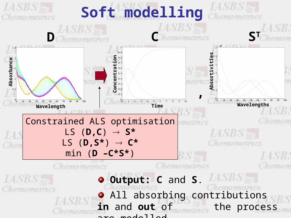
D C
Constrained ALS optimisationLS (D,C) S*LS (D,S*) C*min (D –C*S*)
,
Output: C and S.
All absorbing contributions in and out of the process are modelled.
0 1 2 3 4 5 6 7 8 9 100
0.1
0.2
0.3
0.4
0.5
0.6
0.7
0.8
0.9
1
Time
Co
nc
en
tra
tio
n
Soft modelling
Lecture 1
• Introduction to data structures and soft-modelling methods.
• Factor Analysis of two-way data: Bilinear models.
• Rotation and intensity ambiguities.
• Pseudo-rank, local rank and rank deficiency.
• Evolving Factor Analysis.
Soft-modelling
1 1 2 21
T
.....
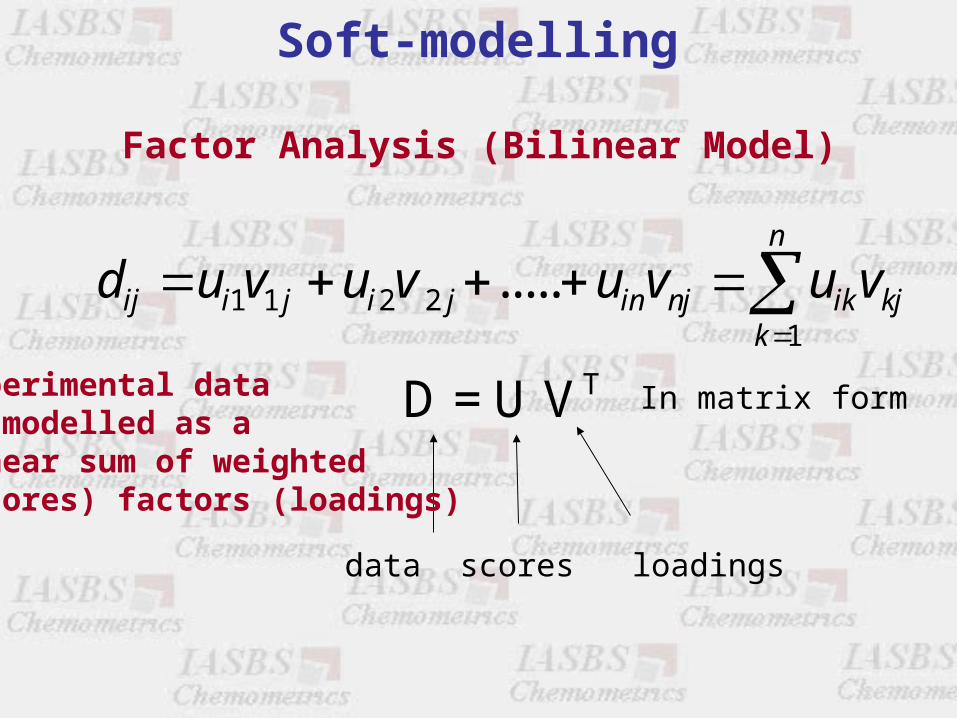
D = U V
n
ij i j i j in nj ik kjk
d u v u v u v u v
In matrix form
data scores loadings
experimental datais modelled as alinear sum of weighted(scores) factors (loadings)
Factor Analysis (Bilinear Model)
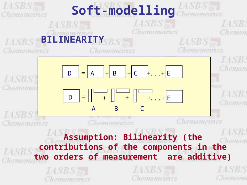
D = + + + ... +A B C E
D =
A
+
B
+
C
+ ... + E+ +
BILINEARITY
Assumption: Bilinearity (the contributions of the components in the two orders of measurement
are additive)
Soft-modelling
0 50 100
0
0.05
0.1
0.15
0.2
0.25
0.3
0.35
0 20 40 60
0
0.05
0.1
0.15
0.2
0.25
0.3
0.35
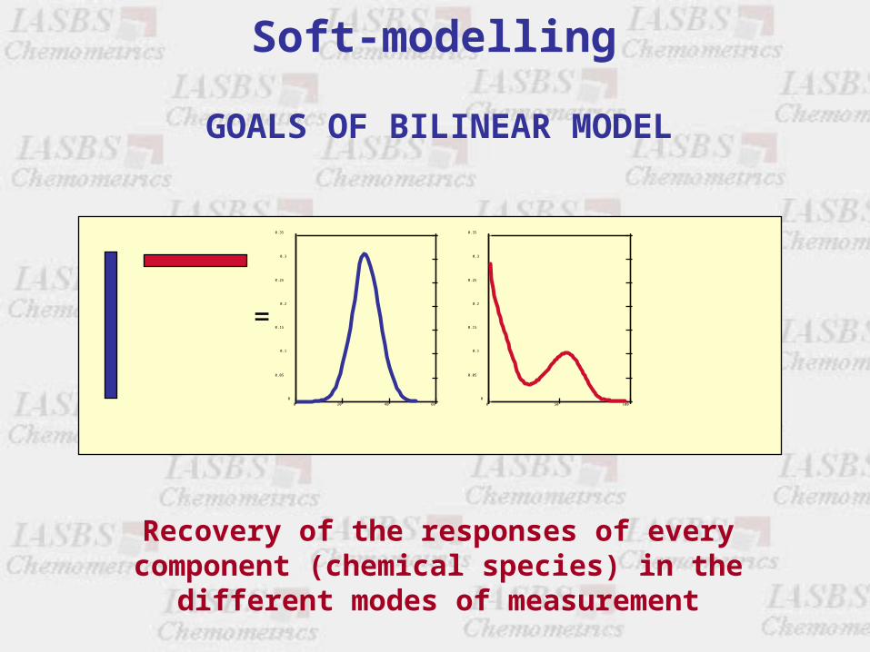
Recovery of the responses of every component (chemical species) in the different modes of
measurement
GOALS OF BILINEAR MODEL
=
Soft-modelling
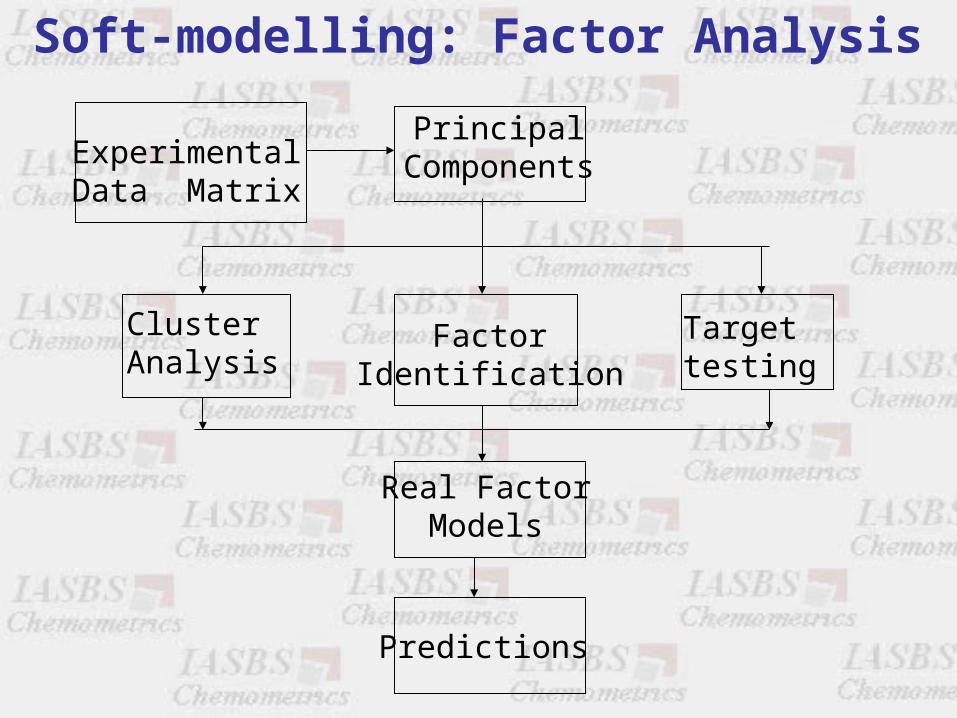
Soft-modelling: Factor Analysis
ExperimentalData Matrix
PrincipalComponents
FactorIdentification
Targettesting
ClusterAnalysis
Real FactorModels
Predictions
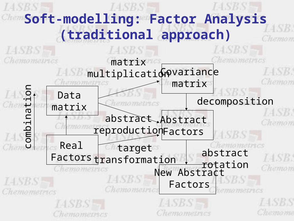
Covariancematrix
AbstractFactors
New AbstractFactors
Datamatrix
RealFactors
com
bina
tion
matrixmultiplication
abstractreproduction
targettransformation
decomposition
abstract rotation
Soft-modelling: Factor Analysis(traditional approach)
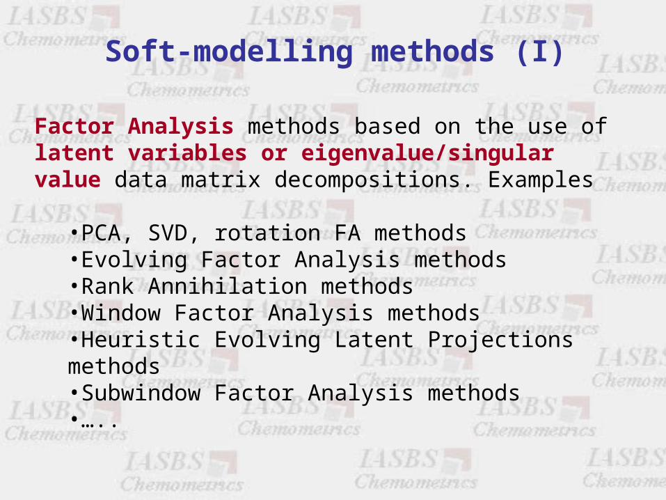
Soft-modelling methods (I)
Factor Analysis methods based on the use of latent variables or eigenvalue/singular value data matrix decompositions. Examples
•PCA, SVD, rotation FA methods•Evolving Factor Analysis methods•Rank Annihilation methods•Window Factor Analysis methods•Heuristic Evolving Latent Projections methods•Subwindow Factor Analysis methods•…..
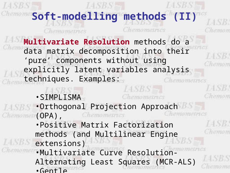
Multivariate Resolution methods do a data matrix decomposition into their ‘pure’ components without using explicitly latent variables analysis techniques. Examples:
•SIMPLISMA•Orthogonal Projection Approach (OPA),•Positive Matrix Factorization methods (and Multilinear Engine extensions)•Multivariate Curve Resolution-Alternating Least Squares (MCR-ALS)•Gentle•.....
Soft-modelling methods (II)
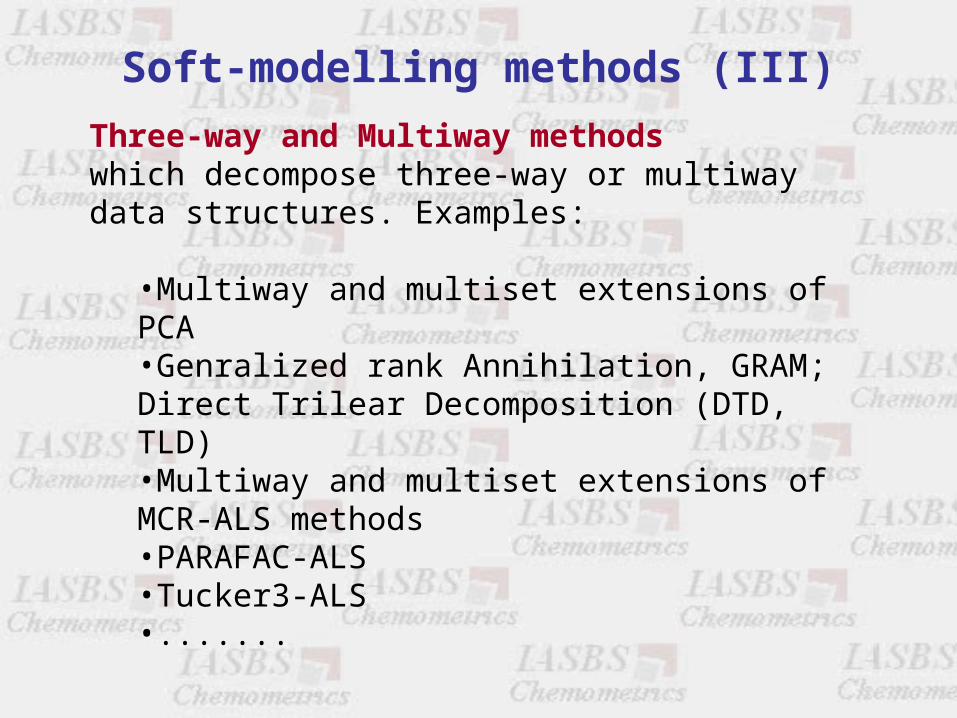
Three-way and Multiway methods which decompose three-way or multiway data structures. Examples:
•Multiway and multiset extensions of PCA•Genralized rank Annihilation, GRAM; Direct Trilear Decomposition (DTD, TLD)•Multiway and multiset extensions of MCR-ALS methods •PARAFAC-ALS•Tucker3-ALS•.......
Soft-modelling methods (III)
Factor Analysis in Chemistry, 3rd Ed., E.R.Malinowski, John Wiley & Sons, New York, 2002
Principal Component Analysis, I.T. Jollife, 2nd Ed., Springer, Berlin, 2002
Multiway Analysis, Applications in the Chemical Sciences, A.Smilde, R.Bro and P.Geladi, John Wiley & Sons, New York, 2004
Multivariate Image Analysis, P.Geladi, John Wiley and Sons, 1996
Soft modeling of Analytical Data. A.de Juan, E.Casassas and R.Tauler, Encyclopedia of Analytical Chemistry: Instrumentation and Applications, Edited by R.A.Meyers, John Wiley & Sons, 2000, Vol 11, 9800-9837
Soft-modelling
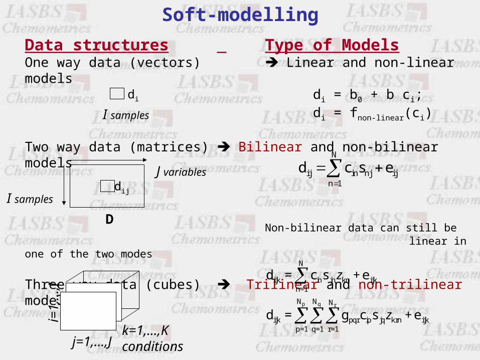
Data structures Type of ModelsOne way data (vectors) Linear and non-linear models
di = b0 + b ci;di = fnon-linear(ci)
Two way data (matrices) Bilinear and non-bilinear models
Non-bilinear data can still belinear in one of the two modes
Three-way data (cubes) Trilinear and non-trilinear models
Non-trilinear data can still be bilinear in two modes
N
ij in nj ijn 1
d c s e
D
I samplesdij
J variables
di
pqr
c
g c
z
zp q r
N
ijk in jn kn ijkn=1
N N N
ijk ip jq krn ijkp=1 q=1 r=1
d = s +e
d = s +ek=1,...,Kconditions
i=1,
...,I
j=1,...,J
I samples
Soft-modelling
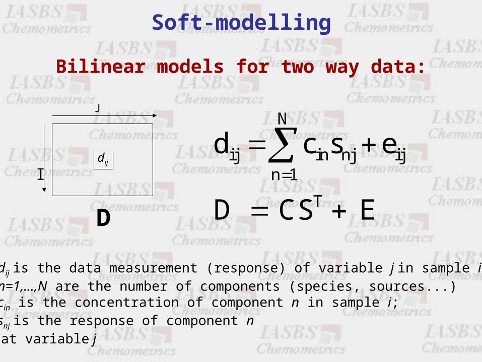
N
ij in nj ijn 1
T
d c s e
D CS E
dij is the data measurement (response) of variable j in sample in=1,...,N are the number of components (species, sources...)cin is the concentration of component n in sample i;snj is the response of component n at variable j
Bilinear models for two way data:
D
J
Idij
Soft-modelling
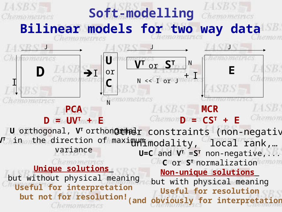
N
DUor
C
VT or ST
E+
J J J
I I
N
N << I or J
Bilinear models for two way data
PCAD = UVT + E
U orthogonal, VT orthonormalVT in the direction of maximum
variance
Unique solutions but without physical meaning
Useful for interpretationbut not for resolution!
MCRD = CST + E
Other constraints (non-negativity,unimodality, local rank,… )
U=C and VT =ST non-negative,...C or ST normalization
Non-unique solutions but with physical meaning
Useful for resolution(and obviously for interpretation)!
I
Soft-modelling
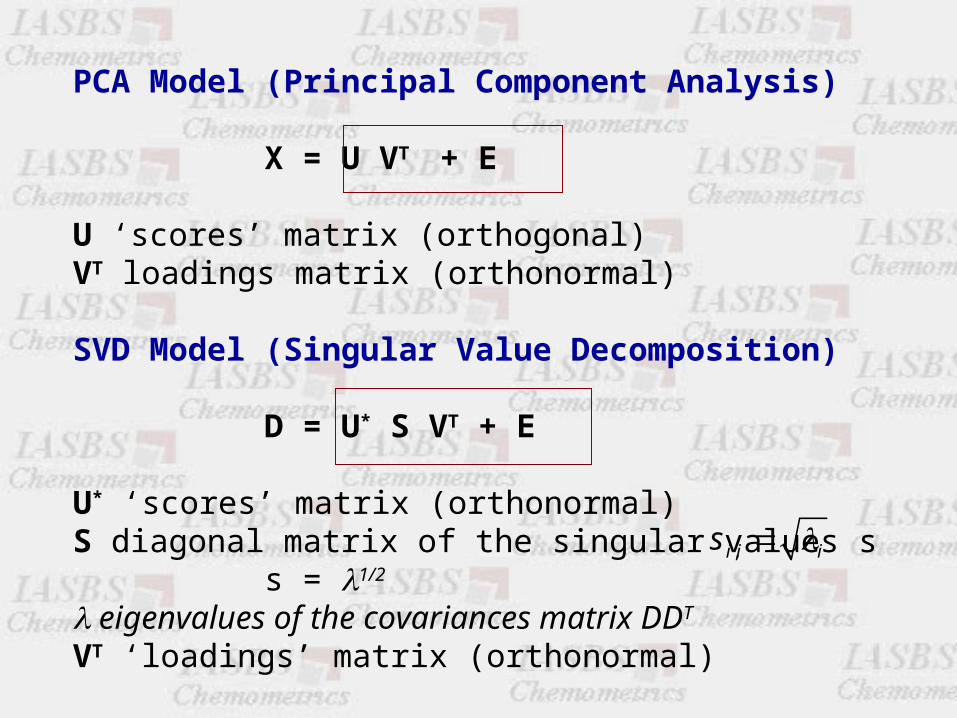
PCA Model (Principal Component Analysis)
X = U VT + E
U ‘scores’ matrix (orthogonal)VT loadings matrix (orthonormal)
SVD Model (Singular Value Decomposition)
D = U* S VT + E
U* ‘scores’ matrix (orthonormal)S diagonal matrix of the singular values s
s = 1/2
eigenvalues of the covariances matrix DDT
VT ‘loadings’ matrix (orthonormal)
,i i is
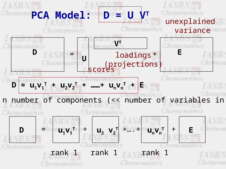
PCA Model: D = U VT
= +DU
VT
E
D = u1v1T + u2v2
T + ……+ unvnT + E
D u1v1T u2 v2
T unvnT E= + +….+ +
n number of components (<< number of variables in D)
rank 1 rank 1 rank 1
scores
loadings(projections)
unexplained variance
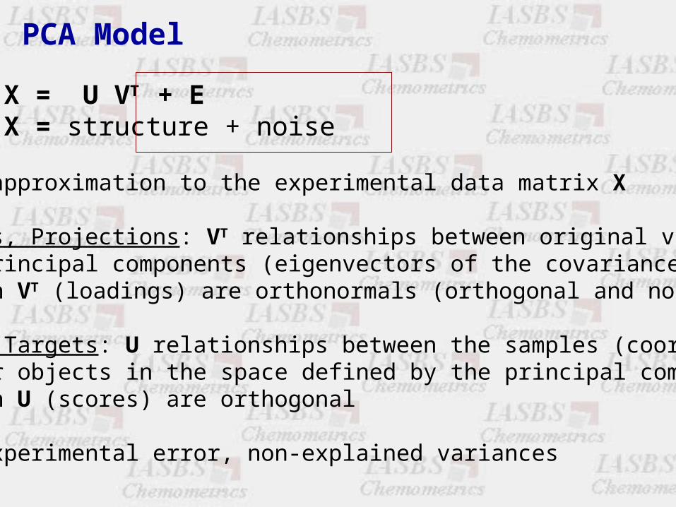
PCA Model
X = U VT + EX = structure + noise
It is an approximation to the experimental data matrix X
• Loadings, Projections: VT relationships between original variables and the principal components (eigenvectors of the covariances matrix). Vectors in VT (loadings) are orthonormals (orthogonal and normalized).
• Scores, Targets: U relationships between the samples (coordinates ofsamples or objects in the space defined by the principal componentsVectors in U (scores) are orthogonal
Noise E Experimental error, non-explained variances
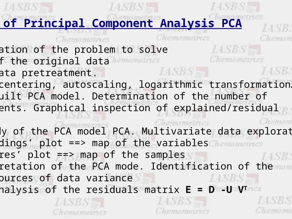
Summary of Principal Component Analysis PCA
1. Formulation of the problem to solve2. Plot of the original data 3. Data pretreatment.
(data centering, autoscaling, logarithmic transformation…)4. Built PCA model. Determination of the number of
components. Graphical inspection of explained/residual plots)
5. Study of the PCA model PCA. Multivariate data exploration- ‘loadings’ plot ==> map of the variables- ‘scores’ plot ==> map of the samples
6. Interpretation of the PCA mode. Identification of themain sources of data variance
7. Analysis of the residuals matrix E = D -U VT
-2-3
-2-10123
PC
2 (
27
%)
Scores plot
-1
-0.8-0.6-0.4-0.2
00.2
PC
2 (
27
%)
Loadings plot
-1 0 1 2 3 4PC1 (41%)
1 2
3
4 5 6
7
8
910
11
12
13141516
17
18
19
2021
22
1
2
3
-1 -0.5 0 0.5 1PC1 (41%)
1
2
3 4 5
6
7 8 910
11
1213141516
1718
1920
21222324
25
2627
282930
313233
34
35
363738
39
40414243444546
47
48495051
52
5354
5556
5758596061
6263
6465
666768697071
727374
75
76
77
78
79
8081
8283
84
858687
8889
9091 929394
9596
B
A
-2 -1 0 1 2 3 4-3
-2
-1
0
1
2
3
PC1 (41%)
PC
2 (
27
%)
Biplot
1 2 3 4 5 6 7 8 91011121314151617 18192021222324
25 26272829303132333435363738
3940414243444546
47484950 515253545556 5758596061 6263646566676869707172737475767778
7980818283 8485868788899091 9293949596
1 2
3
4 5 6
7
8
910
11
12
13141516
17
18
19
20
21
22
Site 1Site 2Site 3
Site 22
Sa
mp
lin
g
sit
es
[org]1 [org]2 [org]3 [org]96
Pollutant concentrationData set
D
Uscores
VT
loadings
PCA
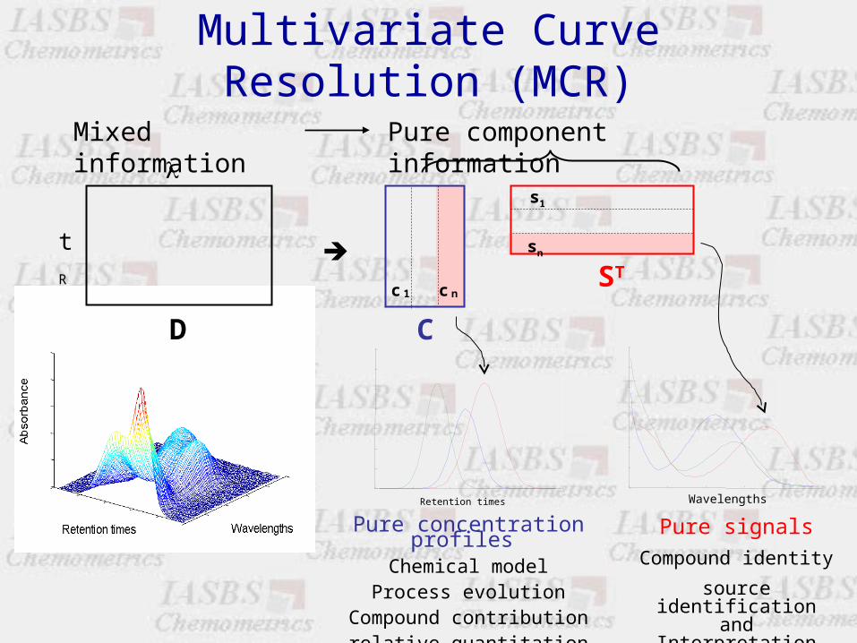
Multivariate Curve Resolution (MCR)
Pure component information
C
ST
sn
s1
c nc 1
WavelengthsRetention times
Pure concentration profiles Chemical model
Process evolutionCompound contribution
relative quantitation
Pure signals
Compound identity
source identification and Interpretation
D
Mixed information
tR
Lecture 1
• Introduction to data structures and soft-modelling methods.
• Factor Analysis of two-way data: Bilinear models.
• Rotation and intensity ambiguities.
• Pseudo-rank, local rank and rank deficiency.
• Evolving Factor Analysis.
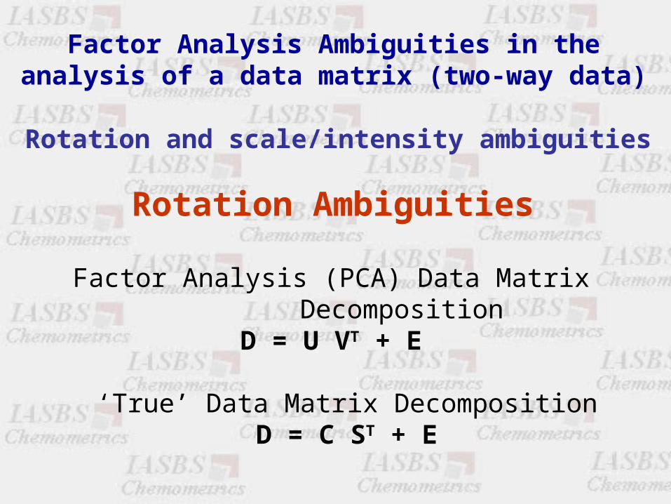
Factor Analysis Ambiguities in the analysis of a data matrix (two-way data)
Rotation Ambiguities
Factor Analysis (PCA) Data Matrix DecompositionD = U VT + E
‘True’ Data Matrix DecompositionD = C ST + E
Rotation and scale/intensity ambiguities
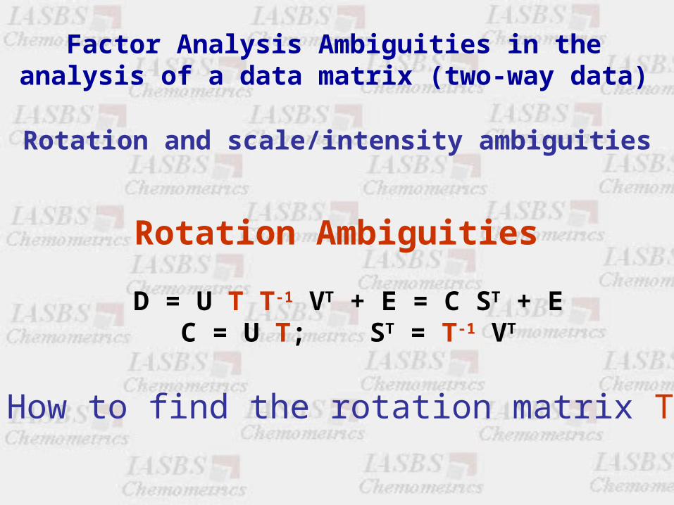
D = U T T-1 VT + E = C ST + EC = U T; ST = T-1 VT
How to find the rotation matrix T?
Factor Analysis Ambiguities in the analysis of a data matrix (two-way data)
Rotation Ambiguities
Rotation and scale/intensity ambiguities
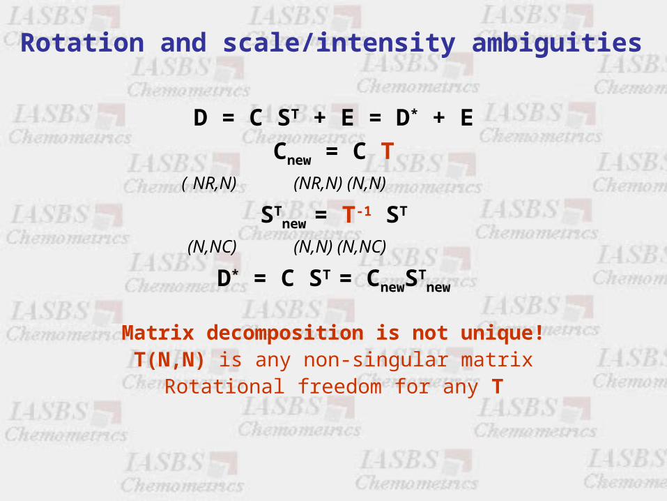
D = C ST + E = D* + E
Cnew = C T ( NR,N) (NR,N) (N,N)
STnew = T-1 ST
(N,NC) (N,N) (N,NC)
D* = C ST = CnewSTnew
Matrix decomposition is not unique!T(N,N) is any non-singular matrix
Rotational freedom for any T
Rotation and scale/intensity ambiguities
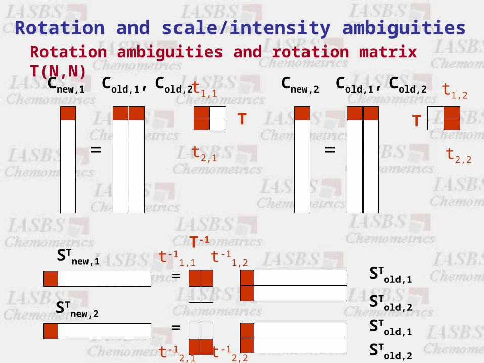
=
Cnew,2 Cold,1, Cold,2 t1,2
t2,2
STnew,1
STold,1
STold,2
STnew,2
t-12,2t-1
2,1
STold,1
STold,2
=
=
T
t-11,1 t-1
1,2
T-1
=
Cnew,1 Cold,1, Cold,2 t1,1
t2,1
T
Rotation and scale/intensity ambiguities
Rotation ambiguities and rotation matrix T(N,N)
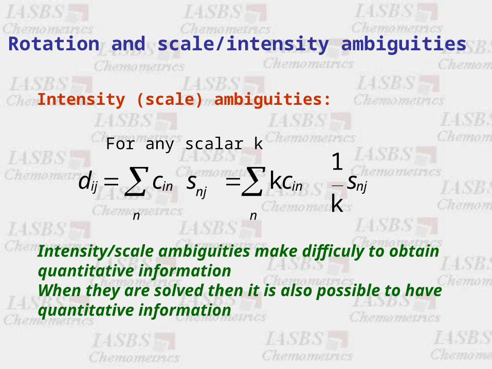
Intensity (scale) ambiguities:
d c s c sij in nj
n
in nj
n
k1
k
For any scalar k
Intensity/scale ambiguities make difficuly to obtain quantitative informationWhen they are solved then it is also possible to have quantitative information
Rotation and scale/intensity ambiguities
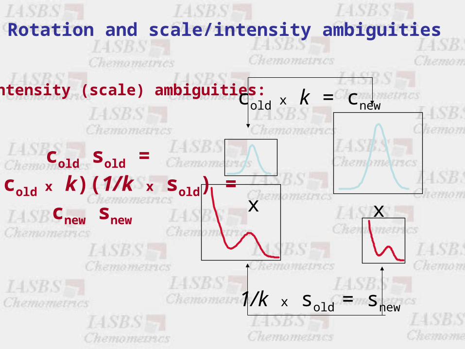
Intensity (scale) ambiguities: cold x k = cnew
x x
1/k x sold = snew
cold sold == ( cold x k)(1/k x sold) =
cnew snew
Rotation and scale/intensity ambiguities
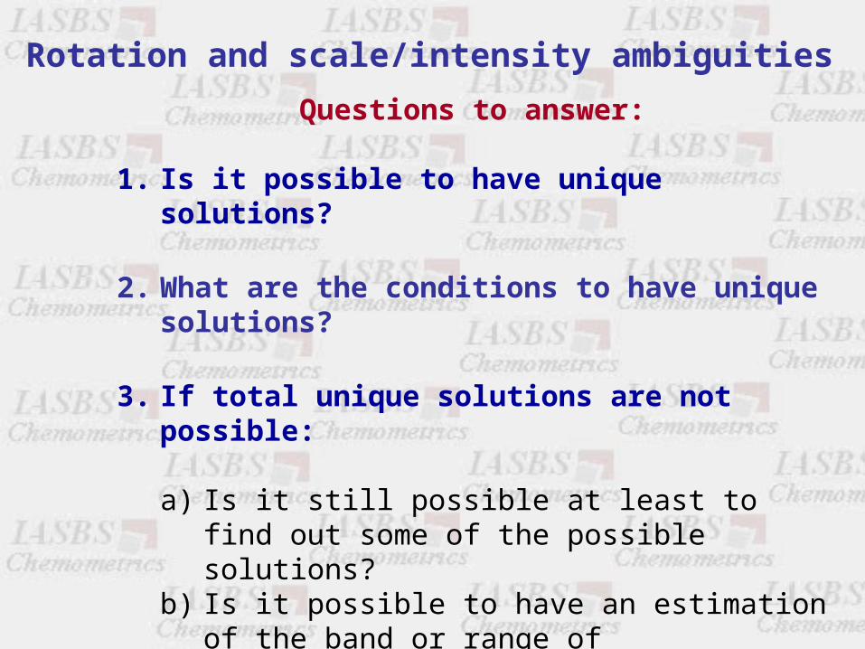
Questions to answer:
1. Is it possible to have unique solutions?
2. What are the conditions to have unique solutions?
3. If total unique solutions are not possible:
a) Is it still possible at least to find out some of the possible solutions?
b) Is it possible to have an estimation of the band or range of possible/feasible solutions?
c) How this range of feasible solutions can be reduced?
Rotation and scale/intensity ambiguities
Lecture 1
• Introduction to data structures and soft-modelling methods.
• Factor Analysis of two-way data: Bilinear models.
• Rotation and intensity ambiguities.
• Pseudo rank, local rank and rank deficiency.
• Evolving Factor Analysis.
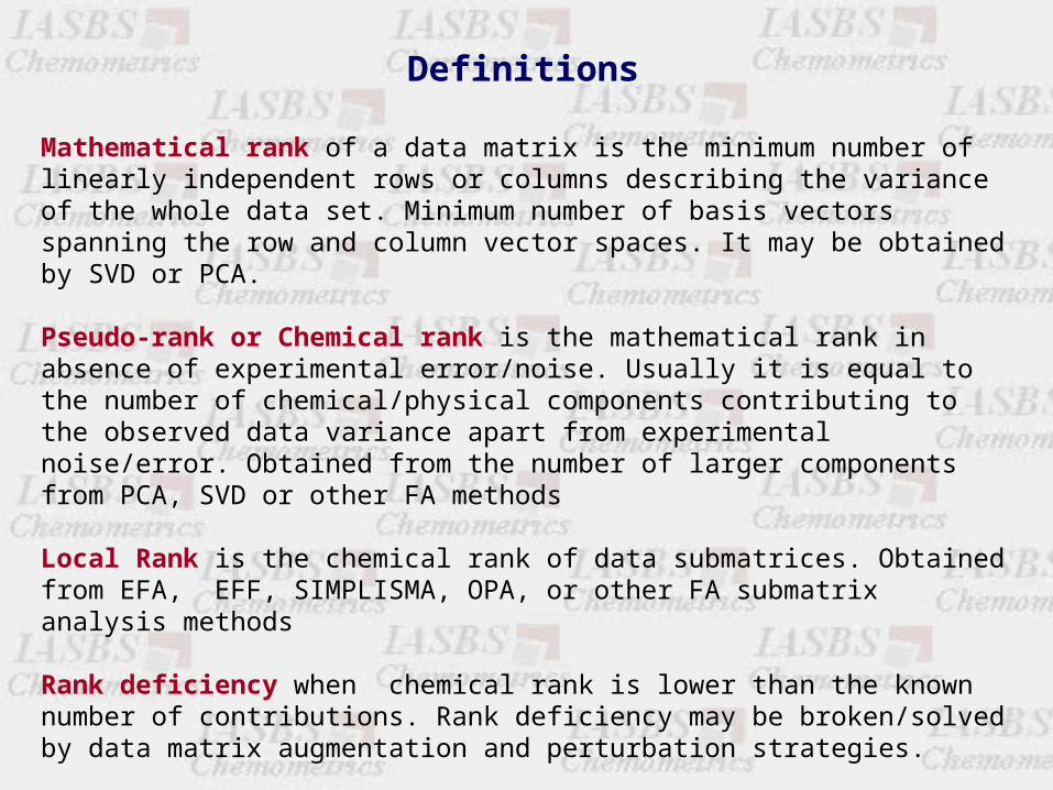
Definitions
Mathematical rank of a data matrix is the minimum number of linearly independent rows or columns describing the variance of the whole data set. Minimum number of basis vectors spanning the row and column vector spaces. It may be obtained by SVD or PCA.
Pseudo-rank or Chemical rank is the mathematical rank in absence of experimental error/noise. Usually it is equal to the number of chemical/physical components contributing to the observed data variance apart from experimental noise/error. Obtained from the number of larger components from PCA, SVD or other FA methods
Local Rank is the chemical rank of data submatrices. Obtained from EFA, EFF, SIMPLISMA, OPA, or other FA submatrix analysis methods
Rank deficiency when chemical rank is lower than the known number of contributions. Rank deficiency may be broken/solved by data matrix augmentation and perturbation strategies.
Rank overlap rank deficiency caused by equal vector profiles of different chemical/physical components in one or more modes.
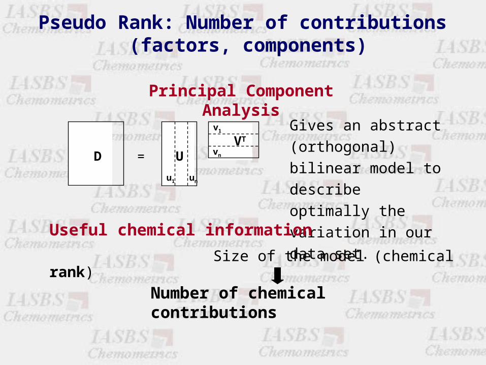
Pseudo Rank: Number of contributions (factors, components)
Principal Component Analysis
D = U
unu1
VT
vn
v1 Gives an abstract
(orthogonal) bilinear
model to describe
optimally the variation
in our data set.Useful chemical information
Size of the model (chemical rank)
Number of chemical contributions
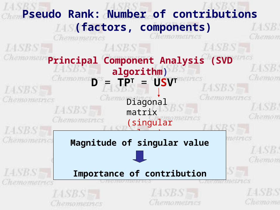
Principal Component Analysis (SVD algorithm)
D = TPT = USVT
Diagonal matrix (singular values)
Magnitude of singular value
Importance of contribution
Pseudo Rank: Number of contributions (factors, components)
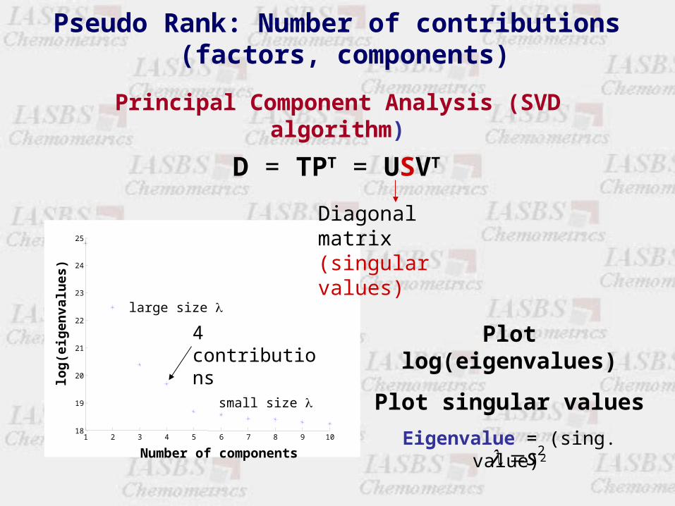
Principal Component Analysis (SVD algorithm)
1 2 3 4 5 6 7 8 9 1018
19
20
21
22
23
24
25
Number of components
log
(eig
en
valu
es)
4 contributions Plot log(eigenvalues)
Plot singular values
Eigenvalue = (sing. value)2
D = TPT = USVT
Diagonal matrix (singular values)
Pseudo Rank: Number of contributions (factors, components)
2s
small size
large size
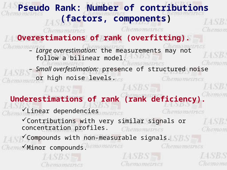
Overestimations of rank (overfitting).
– Large overestimation: the measurements may not follow a bilinear model.
– Small overfestimation: presence of structured noise or high
noise levels.
Underestimations of rank (rank deficiency).
Linear dependencies
Contributions with very similar signals or concentration profiles.
Compounds with non-measurable signals.
Minor compounds.
Pseudo Rank: Number of contributions (factors, components)
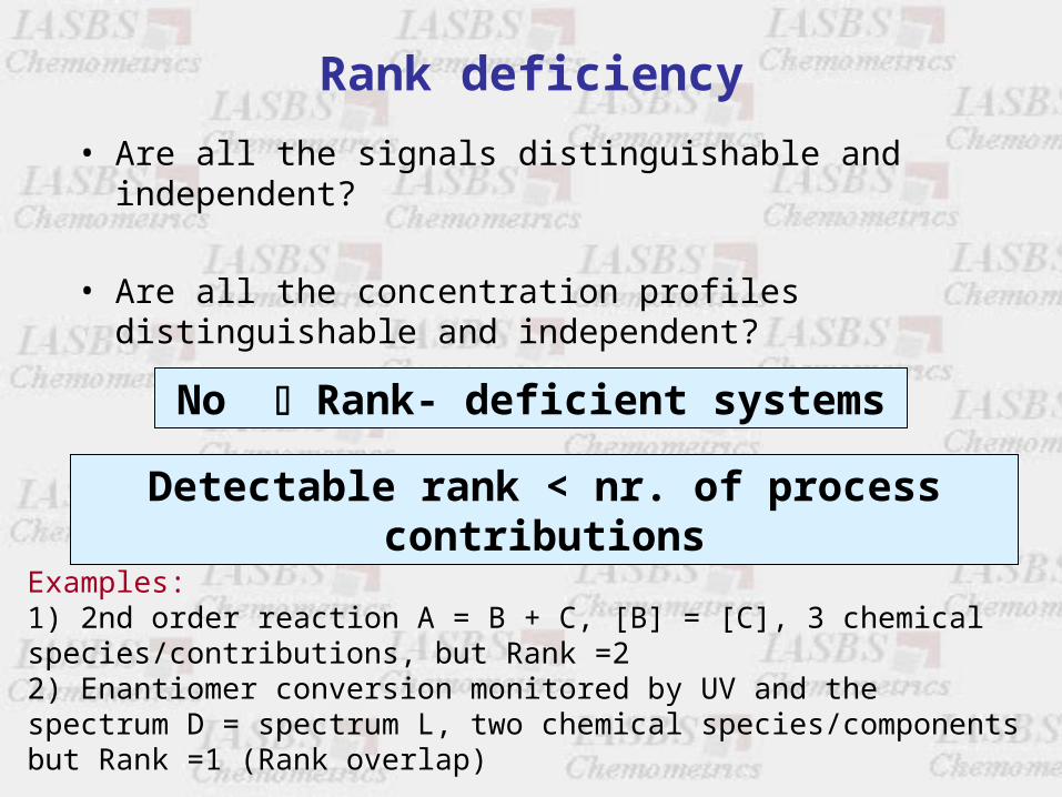
• Are all the signals distinguishable and independent?
• Are all the concentration profiles distinguishable and independent?
No Rank- deficient systems
Rank deficiency
Detectable rank < nr. of process contributions
Examples:1) 2nd order reaction A = B + C, [B] = [C], 3 chemical species/contributions, but Rank =22) Enantiomer conversion monitored by UV and the spectrum D = spectrum L, two chemical species/components but Rank =1 (Rank overlap)
Rank deficiency
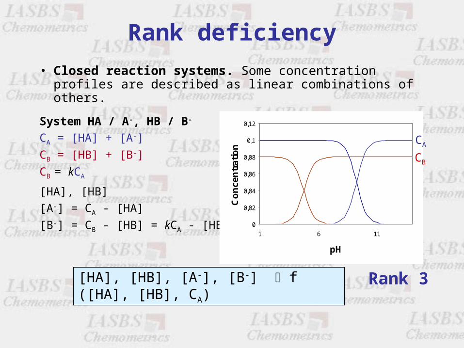
• Closed reaction systems. Some concentration profiles are described as linear combinations of others.
System HA / A-, HB / B-
CA = [HA] + [A-]
CB = [HB] + [B-]
CB = kCA
[HA], [HB]
[A-] = CA - [HA]
[B-] = CB - [HB] = kCA - [HB]
[HA], [HB], [A-], [B-] f ([HA], [HB], CA) Rank 3
0
0,02
0,04
0,06
0,08
0,1
0,12
1 6 11
pH
Co
nce
ntr
atio
n
CA
CB
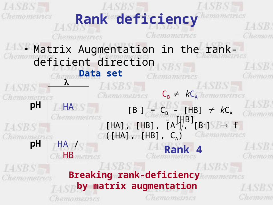
Breaking rank-deficiency by matrix augmentation
• Matrix Augmentation in the rank-deficient direction
Data set
HA
HA / HB
pH
pH
CB kCA
[B-] = CB - [HB] kCA - [HB]
[HA], [HB], [A-], [B-] f ([HA], [HB], CA)
Rank 4
Rank deficiency
Lecture 1
• Introduction to data structures and soft-modelling methods.
• Factor Analysis of two-way data: Bilinear models.
• Rotation and intensity ambiguities.
• Pseudo-rank and rank deficiency.
• Local Rank and Evolving Factor Analysis.
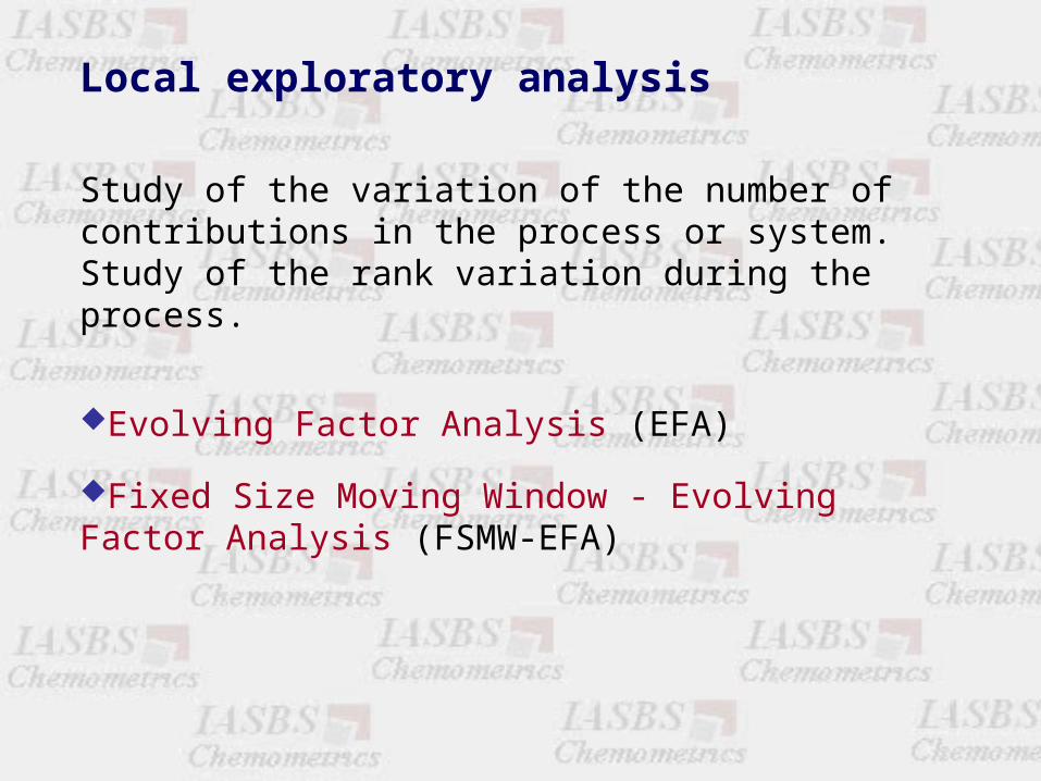
Local exploratory analysis
Study of the variation of the number of contributions in the process or system. Study of the rank variation during the process.
Evolving Factor Analysis (EFA)
Fixed Size Moving Window - Evolving Factor Analysis (FSMW-EFA)
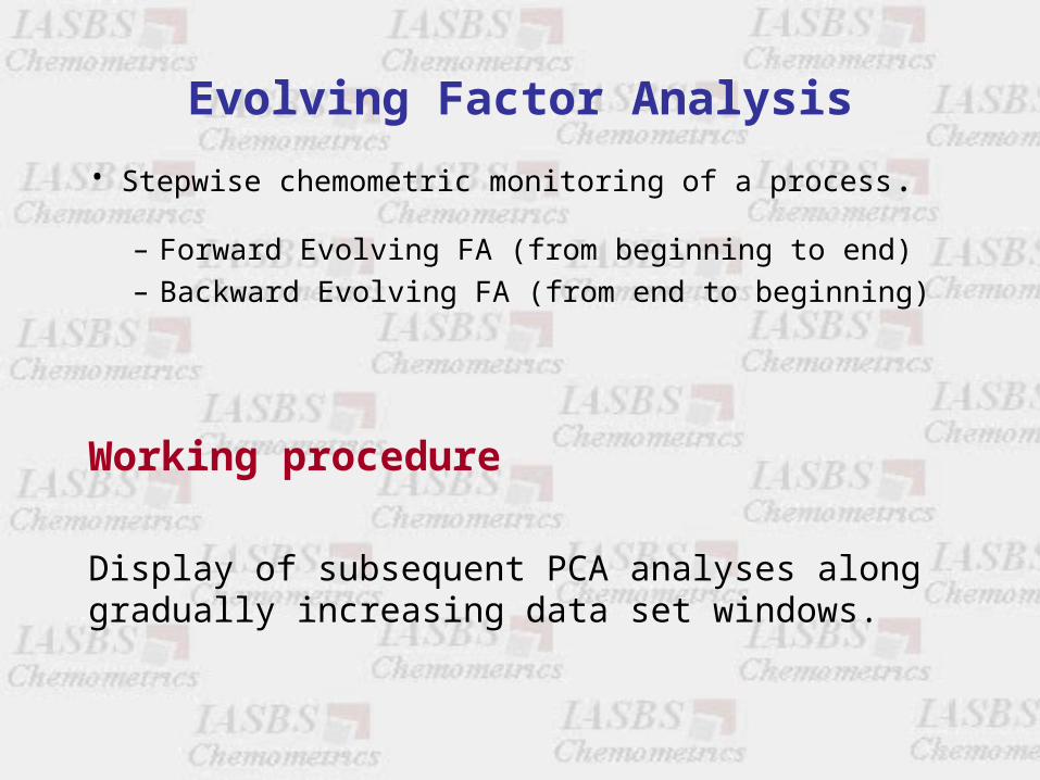
Evolving Factor Analysis
• Stepwise chemometric monitoring of a process.
– Forward Evolving FA (from beginning to end)– Backward Evolving FA (from end to beginning)
Working procedure
Display of subsequent PCA analyses along gradually increasing data set windows.
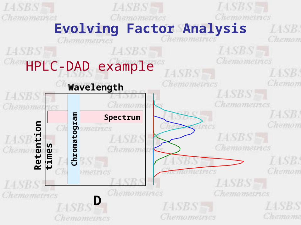
Evolving Factor Analysis
HPLC-DAD example
D
Wavelengths
Ret
enti
on
tim
es
Spectrum
Ch
rom
ato
gra
m
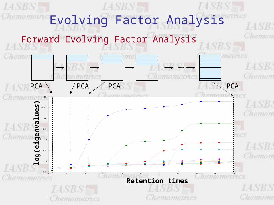
Evolving Factor Analysis
Forward Evolving Factor Analysis
PCA PCA PCA PCA
0 5 10 15 20 25 30 35 40 45 507.5
8
8.5
9
9.5
10
10.5
11
Retention times
log
(eig
enva
lues
)
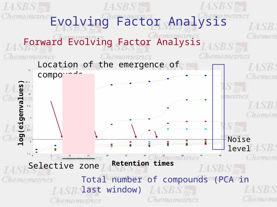
Evolving Factor Analysis
Forward Evolving Factor Analysis
0 5 10 15 20 25 30 35 40 45 507.5
8
8.5
9
9.5
10
10.5
11
Retention times
log
(eig
enva
lues
)
Total number of compounds (PCA in last window)
Noise level
Location of the emergence of compounds
Selective zone
Evolving Factor Analysis
Backward Evolving Factor Analysis
PCAPCAPCAPCA
0 5 10 15 20 25 30 35 40 45 507.5
8
8.5
9
9.5
10
10.5
11
Retention times
log
(eig
en
valu
es)
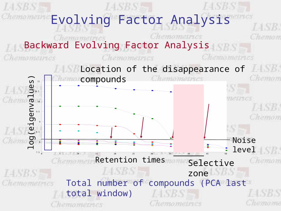
Evolving Factor Analysis
Backward Evolving Factor Analysis
0 5 10 15 20 25 30 35 40 45 507.5
8
8.5
9
9.5
10
10.5
11
Retention times
log
(eig
en
valu
es)
Noise level
Location of the disappearance of compounds
Total number of compounds (PCA last total window)
Selective zone
Evolving Factor Analysis
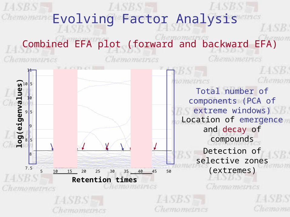
Combined EFA plot (forward and backward EFA)
5 10 15 20 25 30 35 40 45 507.5
8
8.5
9
9.5
10
10.5
11
Retention times
log
(eig
enva
lues
)
Location of emergence and decay of compounds
Detection of selective zones (extremes)
Total number of components (PCA of extreme windows)
Evolving Factor Analysis
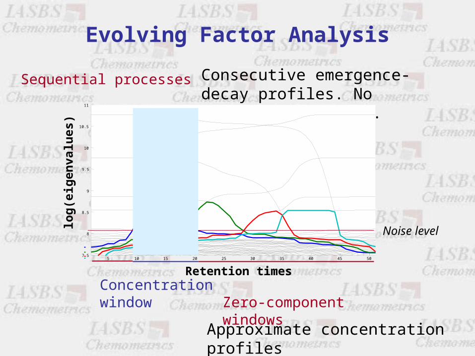
Sequential processes Consecutive emergence-decay profiles. No embedded compounds.
Approximate concentration profiles
Noise level
5 10 15 20 25 30 35 40 45 507.5
8
8.5
9
9.5
10
10.5
11
Retention times
log
(eig
enva
lues
)
Concentration windowZero-component windows
Evolving Factor Analysis
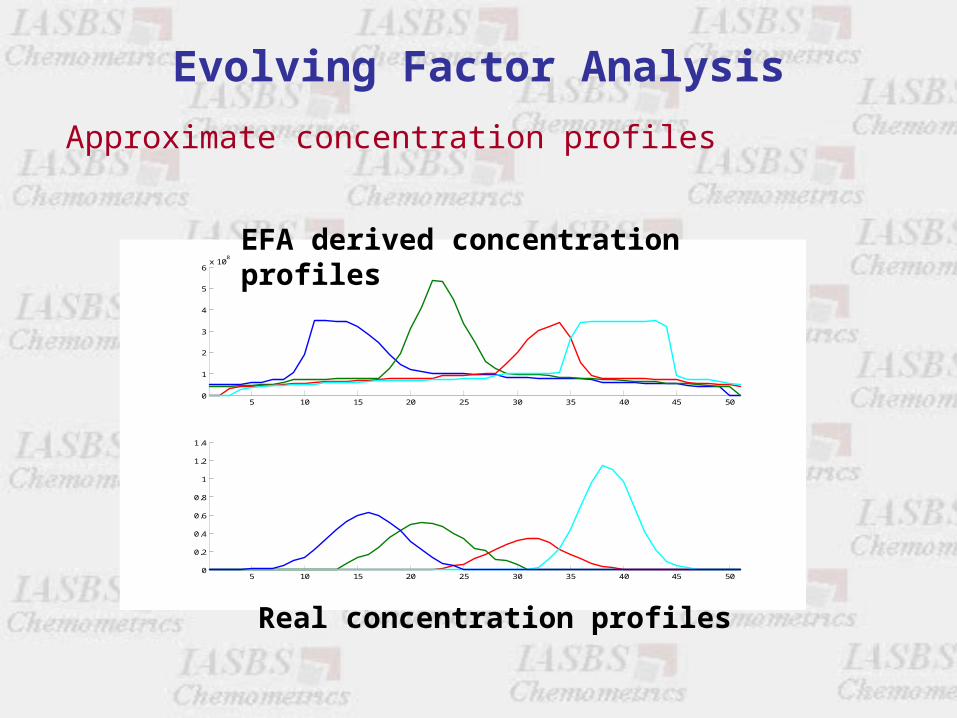
Approximate concentration profiles
5 10 15 20 25 30 35 40 45 500
0.2
0.4
0.6
0.8
1
1.2
1.4
5 10 15 20 25 30 35 40 45 500
1
2
3
4
5
6x 10
8
EFA derived concentration profiles
Real concentration profiles
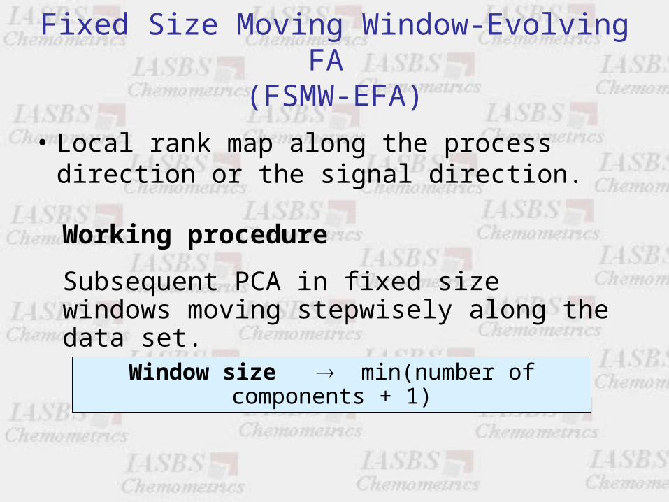
Fixed Size Moving Window-Evolving FA (FSMW-EFA)
• Local rank map along the process direction or the signal direction.
Working procedure
Subsequent PCA in fixed size windows moving stepwisely along the data set.
Window size min(number of components + 1)
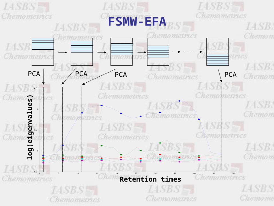
FSMW-EFA
0 5 10 15 20 25 30 35 40 45 503.5
4
4.5
5
5.5
Retention times
log
(eig
enva
lues
)
PCA PCA PCA PCA
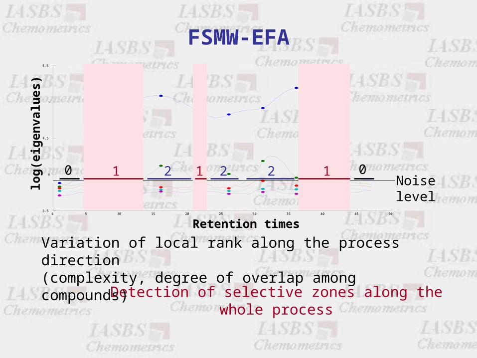
FSMW-EFA
0 5 10 15 20 25 30 35 40 45 503.5
4
4.5
5
5.5
Retention times
log
(eig
enva
lues
)
Noise level
Detection of selective zones along the whole process
10 01 12 22
Variation of local rank along the process direction (complexity, degree of overlap among compounds)
0 20 40 6000.20.40.60.8
11.21.41.61.8
2 x 10 -5
0 20 40 60 80 1000
0.5
1
1.5
2
2.5
3
3.5 x 10⁴
0 20 40 600
0.05
0.1
0.15
0.2
0.25
0.3
0 20 40 60-3
-2
-1
0
1
2
3
0 10 20 30 40 50-2
-1.5
-1
-0.5
0
0.5
1
0 10 20 30 40 50-2
-1.5
-1
-0.5
0
0.5
1
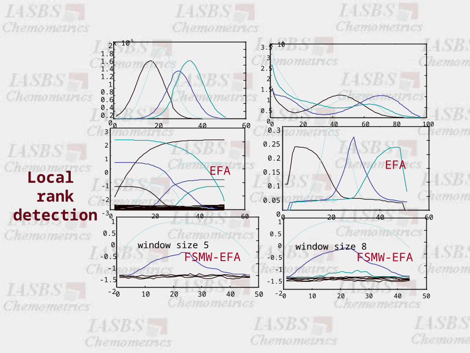
window size 5 window size 8
Local rank
detection
EFAEFA
FSMW-EFA FSMW-EFA
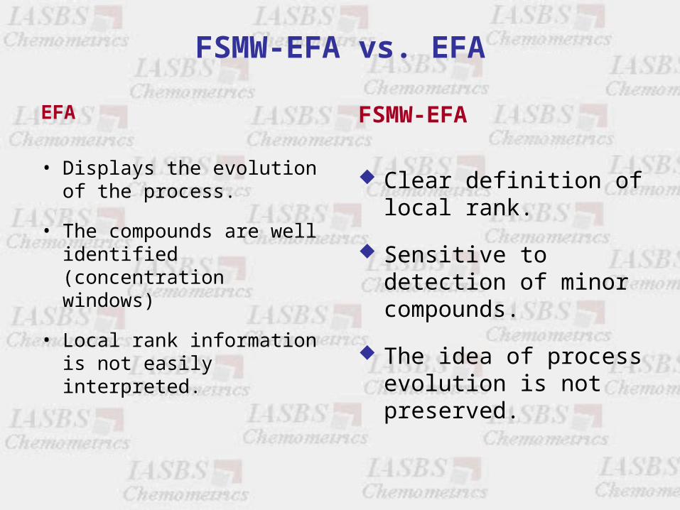
FSMW-EFA vs. EFA
EFA
• Displays the evolution of the process.
• The compounds are well identified (concentration windows)
• Local rank information is not easily interpreted.
FSMW-EFA
Clear definition of local rank.
Sensitive to detection of minor compounds.
The idea of process evolution is not preserved.
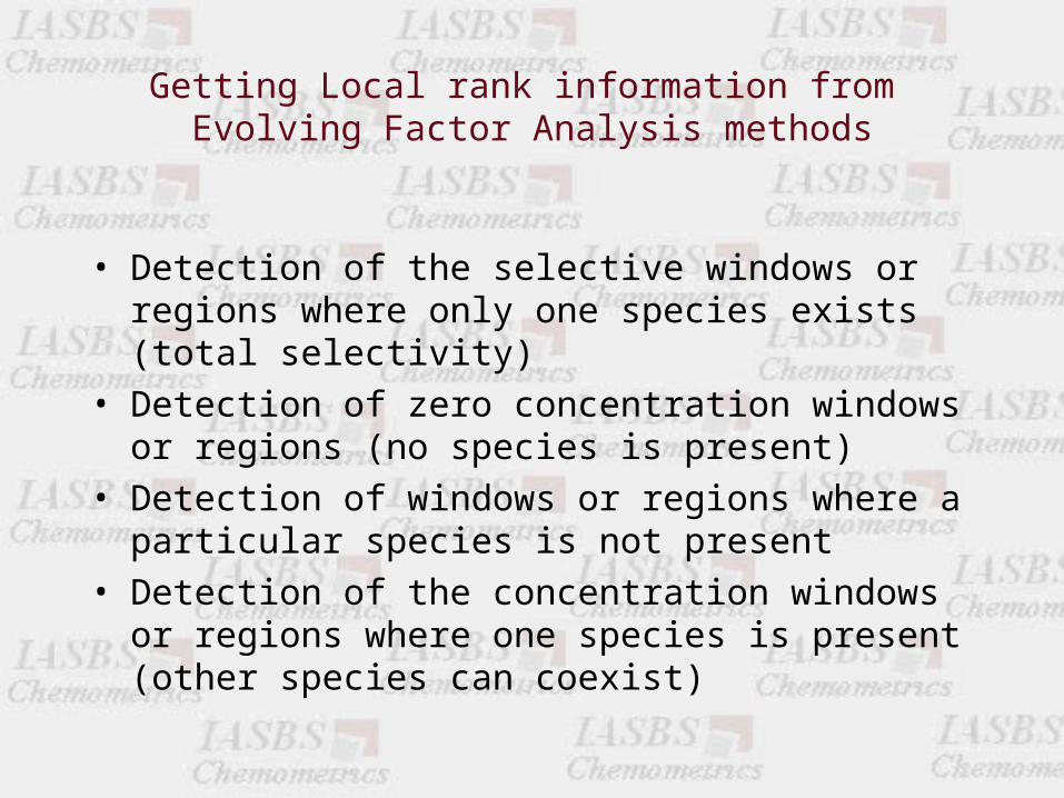
• Detection of the selective windows or regions where only one species exists (total selectivity)
• Detection of zero concentration windows or regions (no species is present)
• Detection of windows or regions where a particular species is not present
• Detection of the concentration windows or regions where one species is present (other species can coexist)
Getting Local rank information from Evolving Factor Analysis methods
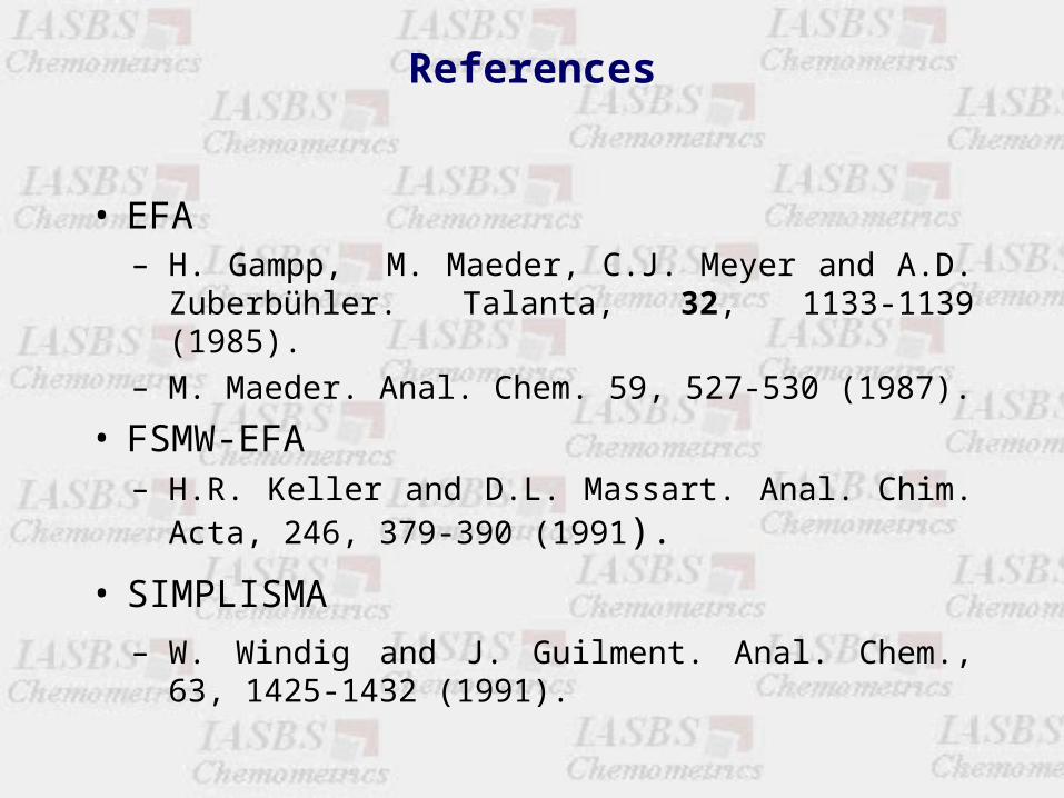
References
• EFA– H. Gampp, M. Maeder, C.J. Meyer and A.D.
Zuberbühler. Talanta, 32, 1133-1139 (1985).– M. Maeder. Anal. Chem. 59, 527-530 (1987).
• FSMW-EFA– H.R. Keller and D.L. Massart. Anal. Chim. Acta,
246, 379-390 (1991).
• SIMPLISMA
– W. Windig and J. Guilment. Anal. Chem., 63, 1425-1432 (1991).
Recommended