FCE III LTER Goals:
Water : How do water
management decisions interact
with climate change to determine
freshwater distribution?
Carbon: How does the balance
of fresh and marine water supplies
regulate C uptake, storage, and
fluxes by influencing water
residence time, nutrient
availability, and salinity?
Legacies: How does historic
variability in the relative supply of
fresh and marine water modify
ecosystem sensitivity to further
change?
Scenarios: What are alternative
socio-ecological futures for South
Florida under contrasting climate
change and water management
scenarios?
B
P
T
O Carbon Cycle
Global
Climate
Change
Global
Socioeconomic
Change
Everglades Coastal Gradient FR
ES
H W
AT
ER
SU
PP
LY
Regional Climate
Modulation
Regional Water
Management and
Land Use
South Florida Urban Gradient
Resource Demand, Use, Stewardship and
Management Decisions
1
MA
RIN
E W
AT
ER
SU
PP
LY
2
1
1
Multi-Scaled Socio-Ecology of the Everglades FCE III Conceptual Framework
4 Past Future
Geochemistry
Primary
Production
Consumers
Organic
Matter
Carbon
Cycle
3 Present
LOCAL RESPONSES
EXTERNAL DRIVERS 1
2
3
4
Socio-ecological feedbacks
Party crashers: displaced marsh
consumers regulate a prey subsidy to
an estuarine consumer
Ross Boucek & Jennifer Rehage
Florida International University [email protected]
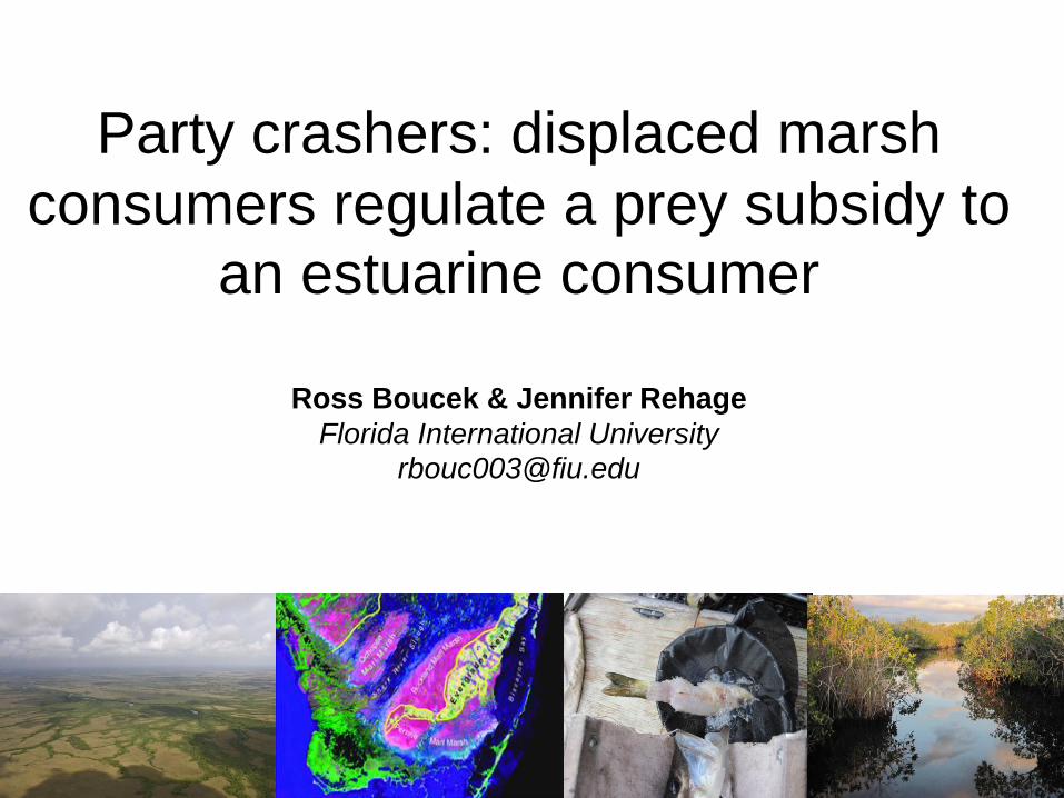
Pulsed resource subsidies
• Resource pulse Instantaneous resource
iincrease (Holt 2008)
• Subsidy Pulses across ecosystem
b boundaries (Anderson et al. 2008)
Yang et al. 2008
Mass emergences
of aquatic insects
Salmon in Pacific
NW
Seaweed deposits
on beaches
Bird guano
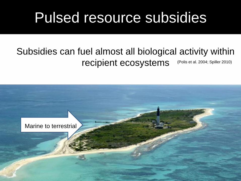
Pulsed resource subsidies
Subsidies can fuel almost all biological activity within
recipient ecosystems
(Polis et al. 2004; Spiller 2010)
Marine to terrestrial

What regulates the flow of resources from one
system to another?
Information gap
Paetzold et al. 2008
?
?
Energy Energy

• Deplete resources locally
– Nothing to transfer (Epichan et al. 2010)
• Track resources across boundaries
– Compete with recipient consumers
Consumers from donor communities important
Paetzold et al. 2008
Energy Energy

In the Pacific Northwest
Ocean
River Salmon migrate up river to spawn
Subsidizing upstream communities

Sea lions Track Salmon Up River
Ocean
River
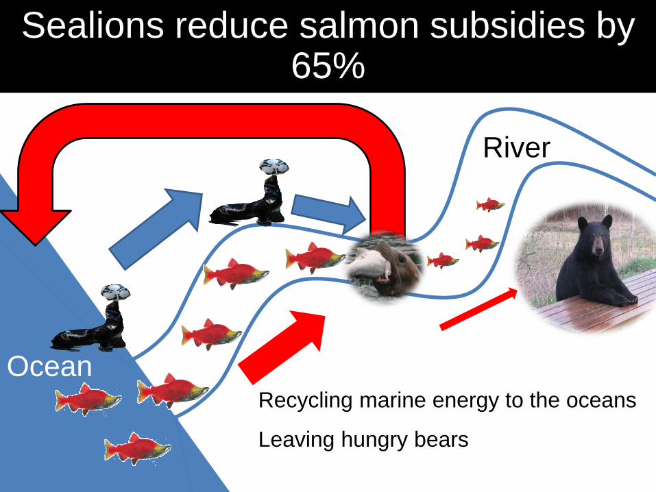
Sealions reduce salmon subsidies by 65%
Ocean
River
Recycling marine energy to the oceans
Leaving hungry bears

Naughton et. al. 2011
Leading to Aggressive Management

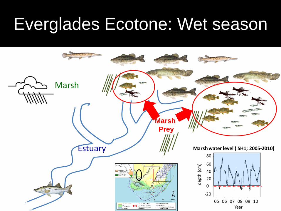
Estuary
Marsh
Everglades Ecotone: Wet season
dep
th (
cm)
80
-20
60
40
20
0
05 06 07 08 09 10
Marsh water level ( SH1; 2005-2010)
Year
Estuary
Marsh
Everglades Ecotone: Wet season
Marsh
Prey
dep
th (
cm)
80
-20
60
40
20
0
05 06 07 08 09 10
Marsh water level ( SH1; 2005-2010)
Year

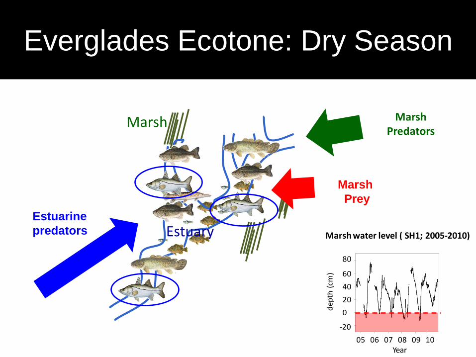
Estuary
Marsh
Everglades Ecotone: Wet season
dep
th (
cm)
80
-20
60
40
20
0
05 06 07 08 09 10
Marsh water level ( SH1; 2005-2010)
Year
Marsh Predators
Marsh
Estuary
Everglades Ecotone: Dry Season
Marsh Predators
Marsh
Prey
Estuarine
predators
dep
th (
cm)
80
-20
60
40
20
0
05 06 07 08 09 10
Marsh water level ( SH1; 2005-2010)
Year

Research questions
(1) Does marsh drying push freshwater prey into the estuary?
(2) How do consumers respond to the pulse?
(3) Are freshwater consumers reducing marsh subsidies for
estuarine consumers?

Focal taxa: 2 freshwater + 1 estuarine
consumer
Largemouth Bass
Gar, bass, bowfin and snook dominate
Consumers show marked seasonality
Wet Early Dry Late Dry
Ele
ctro
fishin
g (
#/1
00m
)
0
2
4
6
8
10
12
14Gar
Bass
Bowfin
Snook
Tarpon
American eel
Gray snapper
Sheepshead
Redfish
Jack crevalle
Ladyfish

Study system: ecotonal sites at ENP
First and second order oligohaline estuarine creeks
< 1.2 m depth
< 10 PSU salinity
600 m
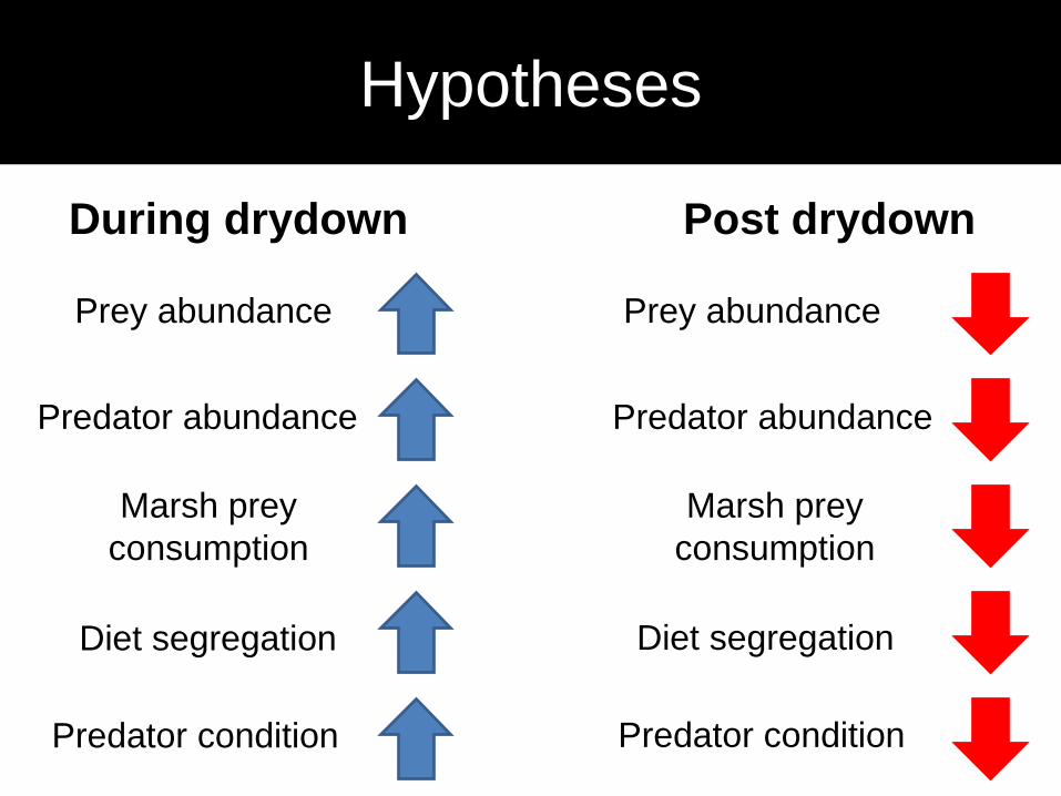
Predator abundance
Hypotheses
Prey abundance
Diet segregation
Predator abundance
Prey abundance
Diet segregation
Marsh prey
consumption
Predator condition Predator condition
During drydown Post drydown
Marsh prey
consumption

Data collection
• Continuously sampled 5 sites
• Nov 2010 to June 2011
• Electrofishing
• Minnow traps
Statistics Compared time & species using GLMs
• Predator abundance
• Prey abundance
4 functional groups
Sunfishes Cyprinodontoids Invertebrates Estuarine prey
Sep Nov Jan Mar May Jul
-1.0
-0.5
0.0
0.5
1.0
1.5
2.0
* * * * * * * * * *
Sep
10
Nov
10
Jan
11
March
11
May
11
July
11
Mar
sh d
ep
th (
cm)
200
100
0
-100
Tracking predator-prey abundance
water level
sampling events *
USGS station SH1
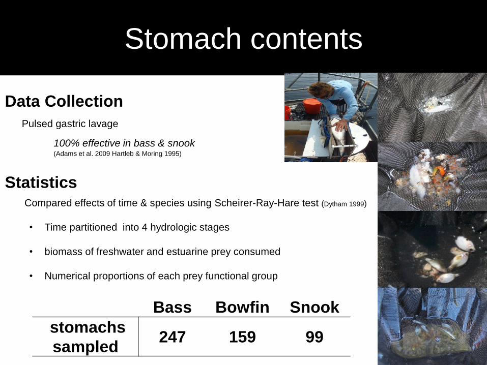
Data Collection
Pulsed gastric lavage
100% effective in bass & snook (Adams et al. 2009 Hartleb & Moring 1995)
Statistics
Compared effects of time & species using Scheirer-Ray-Hare test (Dytham 1999)
• Time partitioned into 4 hydrologic stages
• biomass of freshwater and estuarine prey consumed
• Numerical proportions of each prey functional group
Stomach contents
Bass Bowfin Snook
stomachs
sampled 247 159 99

Nov. Dec. Jan. Feb. Early
Mar.
Late
Mar.
April May June
40
30
20
10
120
40
80
0
# o
f fish p
er
100 m
Not sampled
Electrofishing
Minnow traps
0
160
Cyprinodontoids
Invertebrates
Prey Predators Diet Fitness gains
Species, p = .001
Time, p = .001
Species x time, p =.001
Sunfishes
Sunfishes
Estuarine Prey
# o
f pre
y p
er
trap p
air
Cyprinodontoids
Invertebrates
Estuarine prey
Estuarine prey

# o
f pre
y p
er
trap p
air
Cyprinodontoids
Invertebrates
Nov. Dec. Jan. Feb. Early
Mar.
Late
Mar.
April May June
Sunfishes 40
30
20
10
120
40
80
0
200
100
0
# o
f fish p
er
100 m
Mars
h w
ate
r depth
(cm
)
Marsh water level
Electrofishing
Minnow traps
Marsh drying
0
160 200
100
0
-100
-100
Not sampled
USGS station SH1
Species, p = .001
Time, p = .001
Species x Time, p =.001
Estuarine Prey
Estuarine Prey
Prey Predators Diet Fitness gains
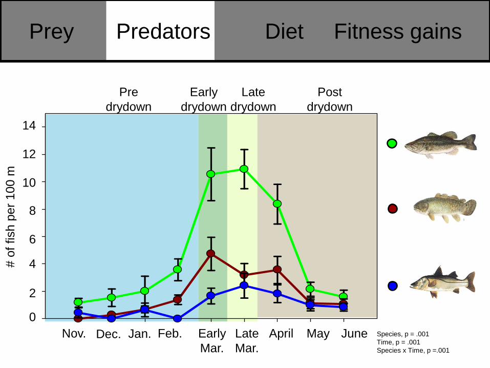
# o
f fish p
er
100 m
10
8
2
0
Nov. Dec. Jan. Feb. Early
Mar.
Late
Mar.
April May June Species, p = .001
Time, p = .001
Species x Time, p =.001
4
6
12
14
Early
drydown
Pre
drydown
Late
drydown
Post
drydown
Prey Predators Diet Fitness gains

0
20
40
60
80
100100
80
60
40
20
0
100
12
8
4
0
Species, p < .001
Time, p < .001
Species x Time, p =.568
Species, p < .001
Time, p = .2915
Species x Time, p =.965
Pre
drydown Early
drydown
Post
drydown
Late
drydown
Freshwater prey
Estuarine prey
Bio
mass (
gra
ms)
consum
ed p
er
100 m
Prey Predators Diet Fitness gains
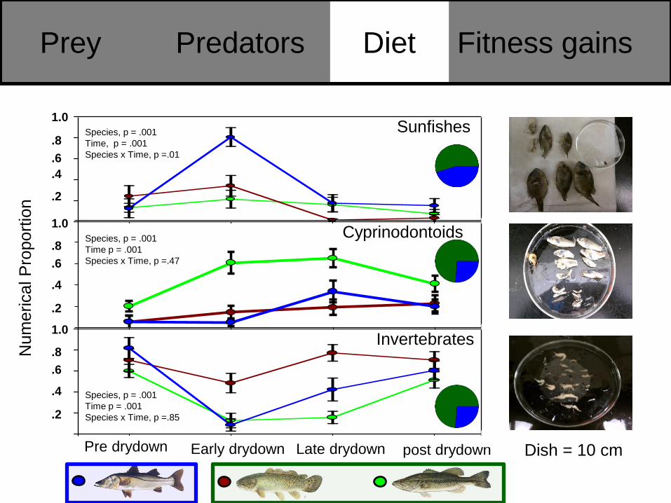
.8
.6
.4
.2
1.0 Sunfishes
Pre drydown Early drydown post drydown Late drydown
0.0
0.2
0.4
0.6
0.8
1.0
Cyprinodontoids
Invertebrates .8
.6
.4
.2
1.0
.8
.6
.4
.2
1.0
Species, p = .001
Time, p = .001
Species x Time, p =.01
Species, p = .001
Time p = .001
Species x Time, p =.47
Species, p = .001
Time p = .001
Species x Time, p =.85
Num
erical P
roport
ion
Dish = 10 cm
Prey Predators Diet Fitness gains

Nov. Dec. Jan. Feb. Early
Mar.
Late
Mar.
April May June Bass, p = .001
Snook, p = .001
Bowfin, p =.001
.03
.025
.02
.015
Conditio
n
.01
* *
* *
*
Prey Predators Diet Fitness gains
Early
drydown
Pre
drydown
Late
drydown
Post
drydown
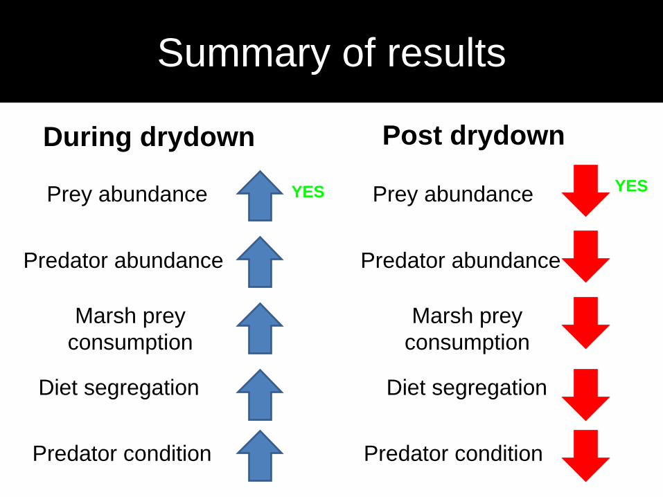
Predator abundance
Prey abundance
Predator abundance
Prey abundance
Marsh prey
consumption
Predator condition Predator condition
During drydown Post drydown
Marsh prey
consumption
YES YES
Summary of results
Diet segregation Diet segregation

Predator abundance
Prey abundance
Predator abundance
Prey abundance
Marsh prey
consumption
Predator condition Predator condition
During drydown Post drydown
Marsh prey
consumption
YES YES
Summary of results
YES YES
Diet segregation Diet segregation
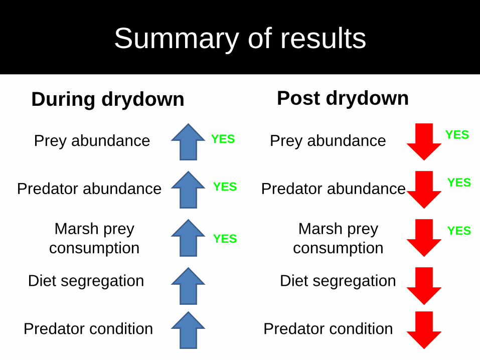
Predator abundance
Prey abundance
Predator abundance
Prey abundance
Diet segregation Diet segregation
Marsh prey
consumption
Predator condition Predator condition
During drydown Post drydown
Marsh prey
consumption
YES YES
Summary of results
YES YES
YES YES

Predator Abundance
Prey Abundance
Predator Abundance
Prey Abundance
Marsh prey consumption
Diet Segregation Diet Segregation
During Drydown Post Drydown
Summary of results
YES YES
YES YES
YES
YES YES
Marsh prey consumption YES

Predator abundance
Prey abundance
Predator abundance
Prey abundance
Diet segregation Diet segregation
Marsh prey
consumption
Predator condition Predator condition
During drydown Post drydown
Marsh prey
consumption
YES YES
Summary of results
YES YES
YES YES
YES YES
YES YES

Implications
Marsh consumers regulate subsidy
Estuarine consumers
Marsh consumers
59%
36%
5%
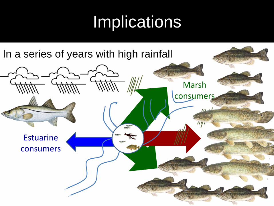
Implications
In a series of years with high rainfall
Estuarine consumers
Marsh consumers
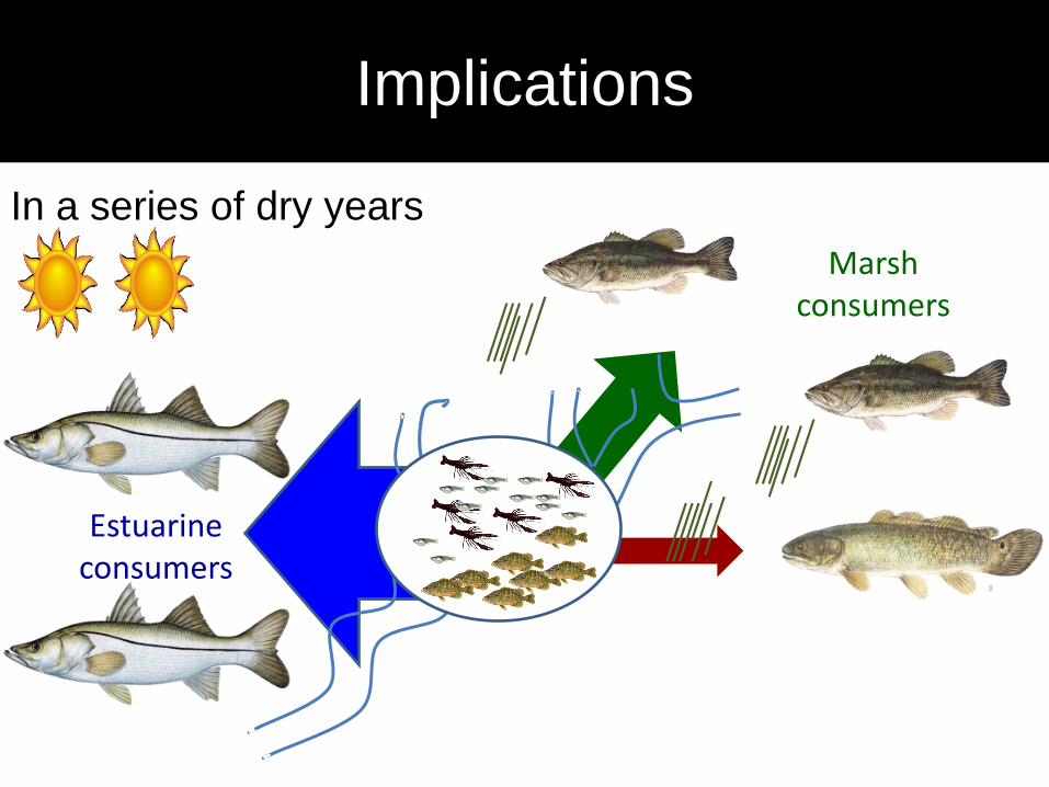
Implications
In a series of dry years
Estuarine consumers
Marsh consumers

19821983
19861987
19881989
19901991
19921993
19941995
19961997
19981999
20002001
20022003
20042005
20062007
20082009
20102011
Angle
r ca
tch p
er
day
0
10
20
30
40 snook
bass
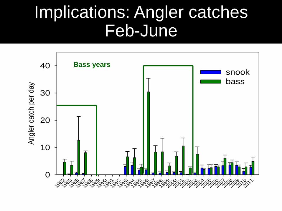
Implications: Angler catches, Feb-June
Recaptured bass!!
Fished nearly every full moon of every month at the Rookery branch since 1982 Anglers in group wear counters to record bass and snook caught per day. Using similar lures since 1982
19821983
19861987
19881989
19901991
19921993
19941995
19961997
19981999
20002001
20022003
20042005
20062007
20082009
20102011
Angle
r ca
tch p
er
day
0
10
20
30
40snook
bass
Bass years
Implications: Angler catches Feb-June

19821983
19861987
19881989
19901991
19921993
19941995
19961997
19981999
20002001
20022003
20042005
20062007
20082009
20102011
Angle
r ca
tch p
er
day
0
10
20
30
40snook
bass
Snook years
Implications: Angler catches, Feb - June
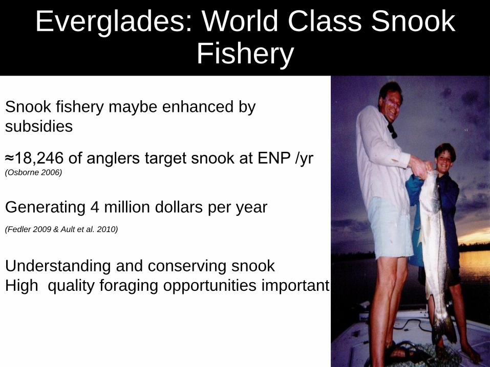
≈18,246 of anglers target snook at ENP /yr (Osborne 2006)
Generating 4 million dollars per year
(Fedler 2009 & Ault et al. 2010)
Understanding and conserving snook
High quality foraging opportunities important
Everglades: World Class Snook Fishery
Snook fishery maybe enhanced by
subsidies
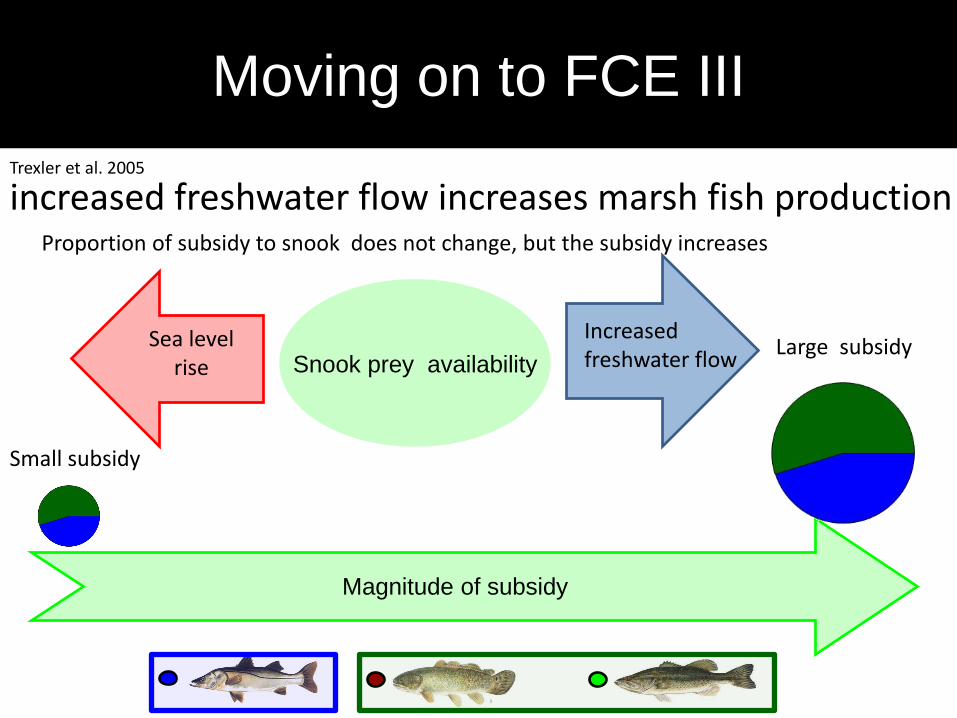
increased freshwater flow increases marsh fish production
Moving on to FCE III
Magnitude of subsidy
Small subsidy
Increased freshwater flow
Large subsidy Snook prey availability
Sea level rise
Proportion of subsidy to snook does not change, but the subsidy increases
Trexler et al. 2005
Please Visit Poster #216 Acknowledgements • USGS • RECOVER • FCE LTER • FIU • Rehage Lab • Aaron Adams • Craig Layman • Michael Heithaus • Amy Narducci • Dave Rose and the southernmost bass anglers
Recommended