Multi-Agent Systems
By Anders Simpson-Wolf, Ramanjit Singh, and Michael Tran
3/13/2013
Visual Demonstration
– more info at http://mobots.epfl.ch/
Presentation Overview
• Relevance/Literature Survey
• Definition
• Motivation
• Formulation of Control Problem
• Simulation
Presentation Overview
• Relevance/Literature Survey
• Definition
• Motivation
• Formulation of Control Problem
• Simulation
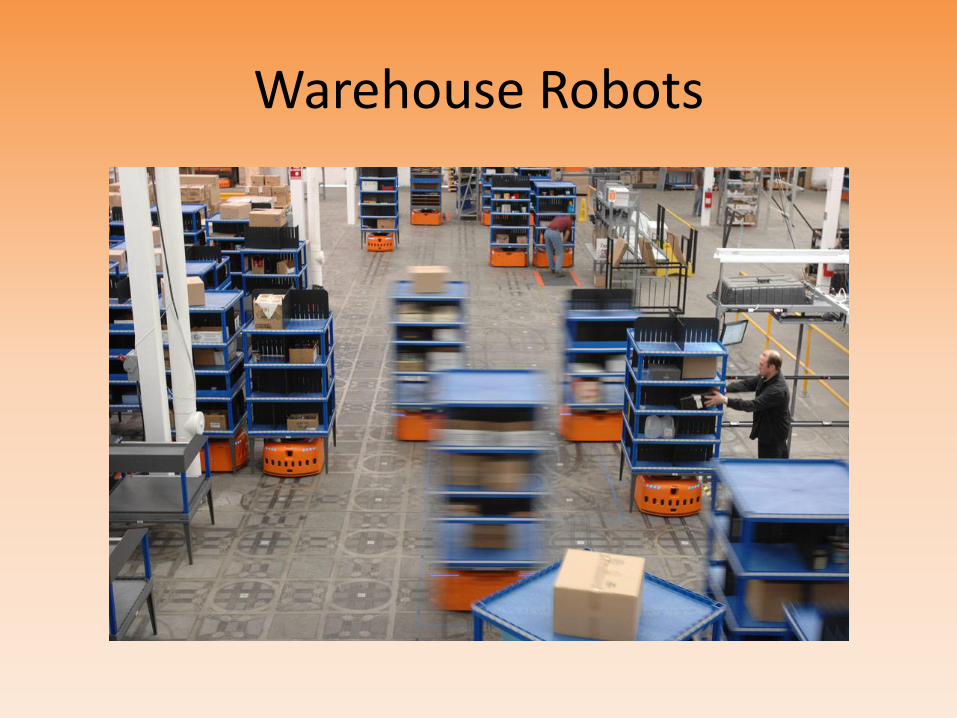
Warehouse Robots
Presentation Overview
• Relevance/Literature Survey
• Definition
• Motivation
• Formulation of Control Problem
• Simulation
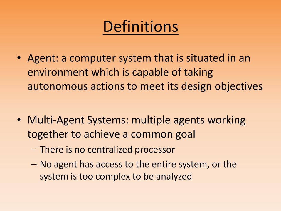
Definitions
• Agent: a computer system that is situated in an environment which is capable of taking autonomous actions to meet its design objectives
• Multi-Agent Systems: multiple agents working together to achieve a common goal
– There is no centralized processor
– No agent has access to the entire system, or the system is too complex to be analyzed
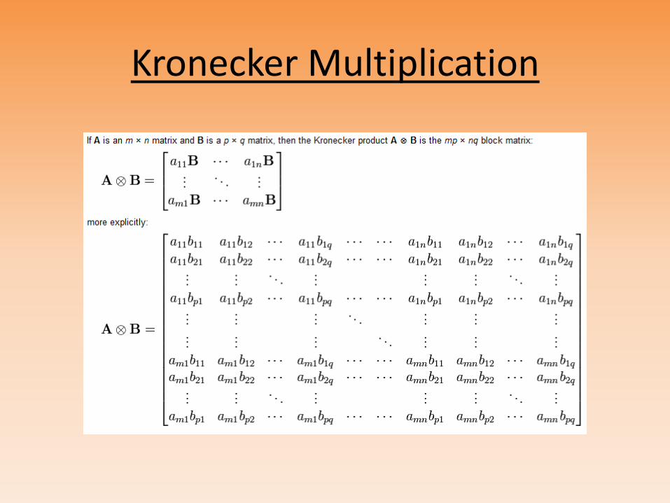
Kronecker Multiplication
Presentation Overview
• Relevance/Literature Survey
• Definition
• Motivation
• Formulation of Control Problem
• Simulation
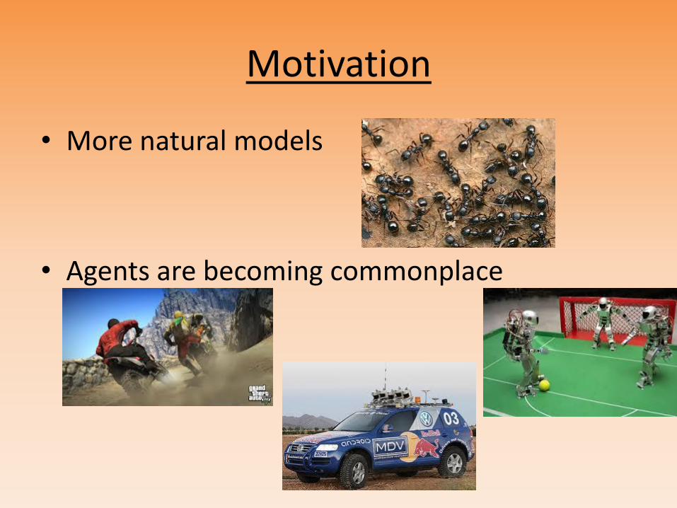
Motivation
• More natural models
• Agents are becoming commonplace
Motivation
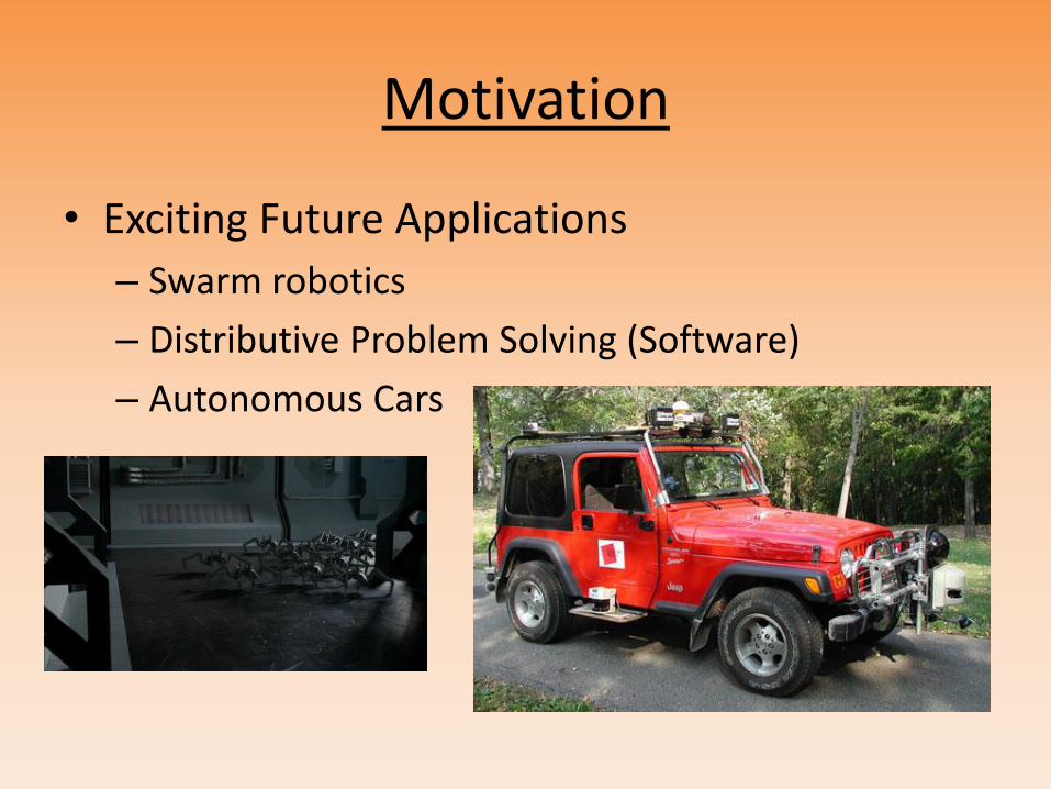
• Exciting Future Applications
– Swarm robotics
– Distributive Problem Solving (Software)
– Autonomous Cars
Presentation Overview
• Relevance/Literature Survey
• Definition
• Motivation
• Formulation of Control Problem
• Simulation
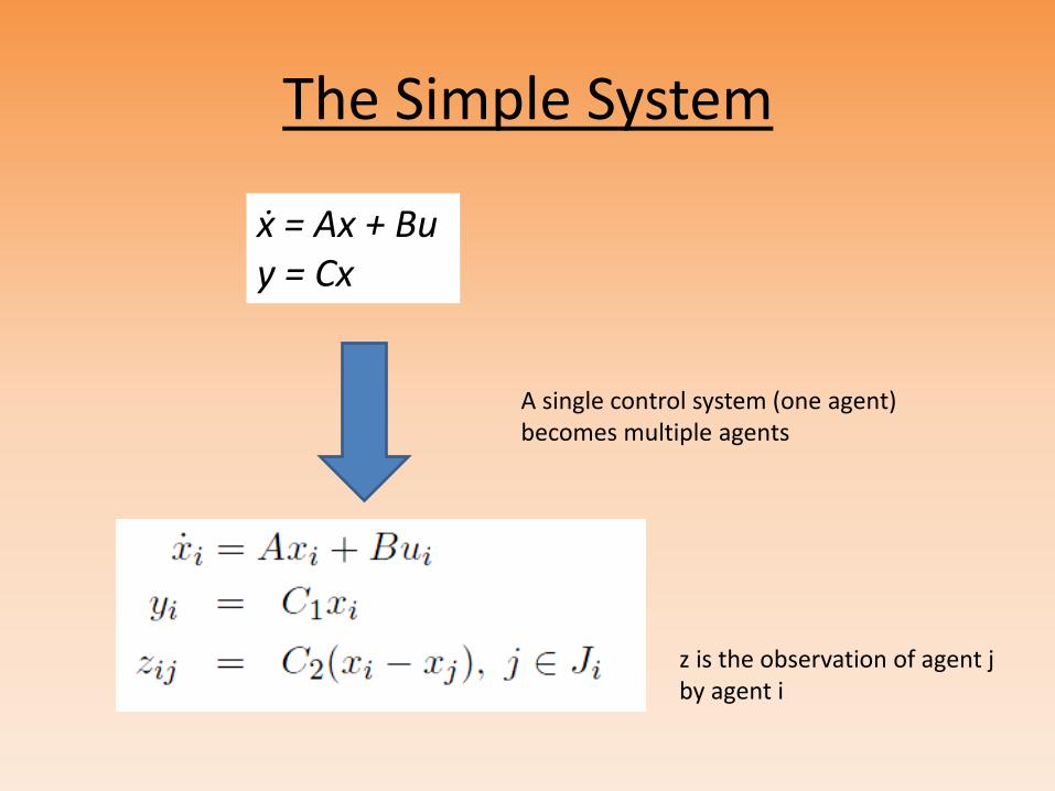
The Simple System
ẋ = Ax + Bu y = Cx
A single control system (one agent) becomes multiple agents
z is the observation of agent j by agent i
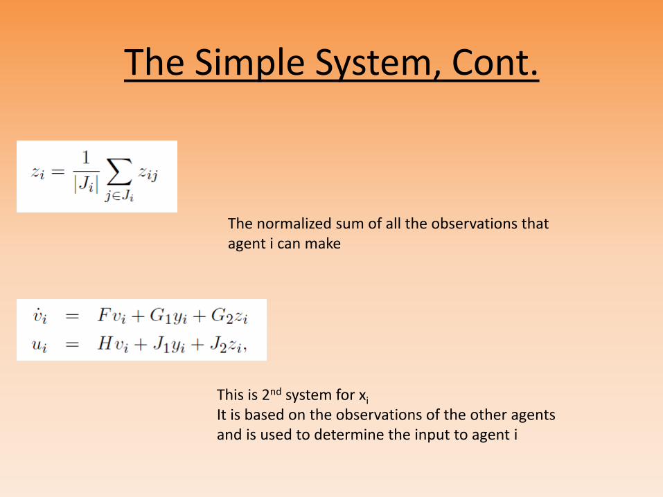
The Simple System, Cont.
The normalized sum of all the observations that agent i can make
This is 2nd system for xi It is based on the observations of the other agents and is used to determine the input to agent i
Application to Vehicles
• Problem Formulation:
– Given N agents, what commands do we send to each in order to arrange the agents in some formation?
• Assumptions:
– Same dynamics for each agent
– Agents are Uncoupled
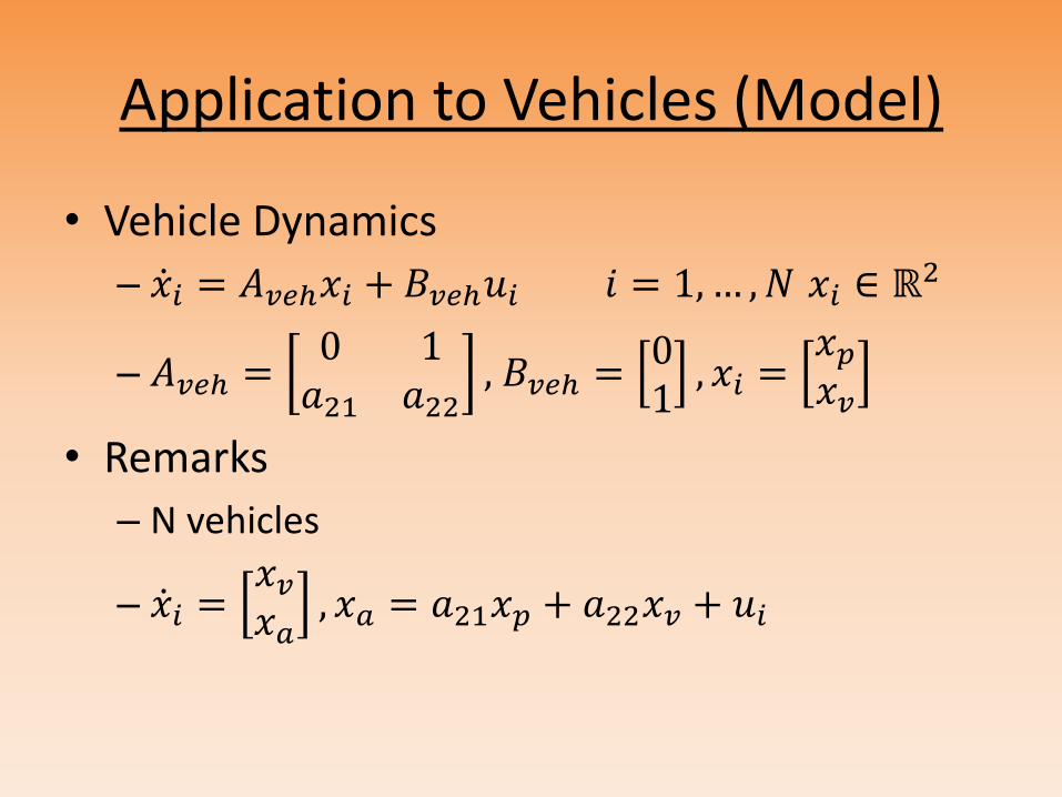
Application to Vehicles (Model)
• Vehicle Dynamics
– 𝑥 𝑖 = 𝐴𝑣𝑒ℎ𝑥𝑖 + 𝐵𝑣𝑒ℎ𝑢𝑖 𝑖 = 1,… , 𝑁 𝑥𝑖 ∈ ℝ2
– 𝐴𝑣𝑒ℎ =0 1𝑎21 𝑎22
, 𝐵𝑣𝑒ℎ =01, 𝑥𝑖 =
𝑥𝑝𝑥𝑣
• Remarks
– N vehicles
– 𝑥 𝑖 =𝑥𝑣𝑥𝑎
, 𝑥𝑎 = 𝑎21𝑥𝑝 + 𝑎22𝑥𝑣 + 𝑢𝑖
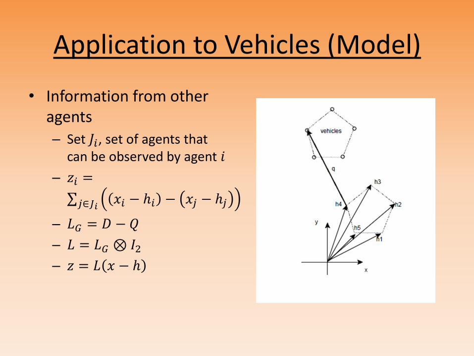
Application to Vehicles (Model)
• Information from other agents
– Set 𝐽𝑖, set of agents that can be observed by agent 𝑖
– 𝑧𝑖 =
𝑥𝑖 − ℎ𝑖 − 𝑥𝑗 − ℎ𝑗𝑗∈𝐽𝑖
– 𝐿𝐺 = 𝐷 − 𝑄
– 𝐿 = 𝐿𝐺 ⊗ 𝐼2
– 𝑧 = 𝐿 𝑥 − ℎ
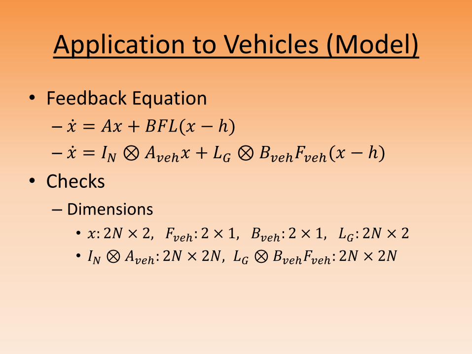
Application to Vehicles (Model)
• Feedback Equation
– 𝑥 = 𝐴𝑥 + 𝐵𝐹𝐿(𝑥 − ℎ)
– 𝑥 = 𝐼𝑁 ⊗𝐴𝑣𝑒ℎ𝑥 + 𝐿𝐺 ⊗𝐵𝑣𝑒ℎ𝐹𝑣𝑒ℎ(𝑥 − ℎ)
• Checks
– Dimensions
• 𝑥: 2𝑁 × 2, 𝐹𝑣𝑒ℎ: 2 × 1, 𝐵𝑣𝑒ℎ: 2 × 1, 𝐿𝐺: 2𝑁 × 2
• 𝐼𝑁 ⊗𝐴𝑣𝑒ℎ: 2𝑁 × 2𝑁, 𝐿𝐺 ⊗𝐵𝑣𝑒ℎ𝐹𝑣𝑒ℎ: 2𝑁 × 2𝑁
Presentation Overview
• Relevance/Literature Survey
• Definition
• Motivation
• Formulation of Control Problem
• Simulation
Simulation
Problem:
– Get three agents to move into a triangular formation
– Each agent starts with a certain position and velocity
Simulation
Assumptions:
– The internal system of each agent is decoupled from the others
– Each agent can observe the positions of the other two and then adjust its own velocity accordingly
– No agent can directly change the velocity of another
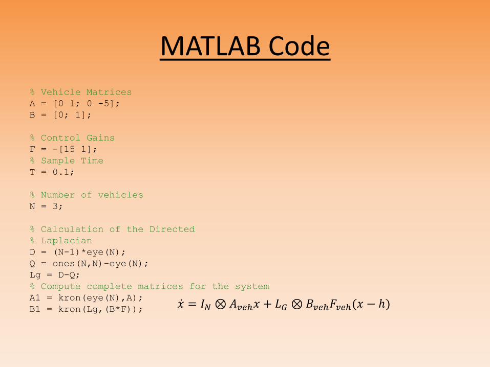
MATLAB Code
% Vehicle Matrices
A = [0 1; 0 -5];
B = [0; 1];
% Control Gains
F = -[15 1];
% Sample Time
T = 0.1;
% Number of vehicles
N = 3;
% Calculation of the Directed
% Laplacian
D = (N-1)*eye(N);
Q = ones(N,N)-eye(N);
Lg = D-Q;
% Compute complete matrices for the system
A1 = kron(eye(N),A);
B1 = kron(Lg,(B*F));
𝑥 = 𝐼𝑁 ⊗𝐴𝑣𝑒ℎ𝑥 + 𝐿𝐺 ⊗𝐵𝑣𝑒ℎ𝐹𝑣𝑒ℎ(𝑥 − ℎ)
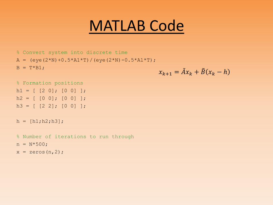
MATLAB Code
% Convert system into discrete time
A = (eye(2*N)+0.5*A1*T)/(eye(2*N)-0.5*A1*T);
B = T*B1;
% Formation positions
h1 = [ [2 0]; [0 0] ];
h2 = [ [0 0]; [0 0] ];
h3 = [ [2 2]; [0 0] ];
h = [h1;h2;h3];
% Number of iterations to run through
n = N*500;
x = zeros(n,2);
𝑥𝑘+1 = 𝐴 𝑥𝑘 + 𝐵 𝑥𝑘 − ℎ
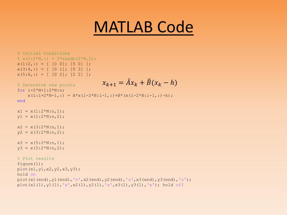
MATLAB Code
% Initial Conditions
% x(1:2*N,:) = 3*randn(2*N,2);
x(1:2,:) = [ [0 0]; [5 0] ];
x(3:4,:) = [ [0 1]; [0 3] ];
x(5:6,:) = [ [0 2]; [2 2] ];
% Determine new points
for i=2*N+1:2*N:n;
x(i:i+2*N-1,:) = A*x(i-2*N:i-1,:)+B*(x(i-2*N:i-1,:)-h);
end
x1 = x(1:2*N:n,1);
y1 = x(1:2*N:n,2);
x2 = x(3:2*N:n,1);
y2 = x(3:2*N:n,2);
x3 = x(5:2*N:n,1);
y3 = x(5:2*N:n,2);
% Plot results
figure(1);
plot(x1,y1,x2,y2,x3,y3);
hold on
plot(x1(end),y1(end),'o',x2(end),y2(end),'o',x3(end),y3(end),'o');
plot(x1(1),y1(1),'x',x2(1),y2(1),'x',x3(1),y3(1),'x'); hold off
𝑥𝑘+1 = 𝐴 𝑥𝑘 + 𝐵 (𝑥𝑘 − ℎ)
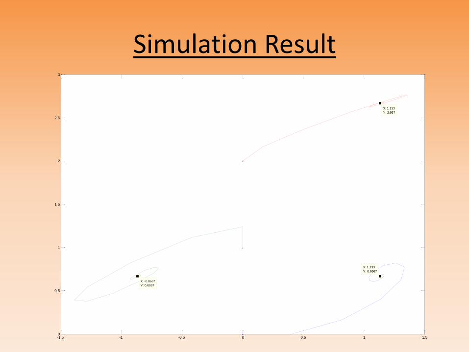
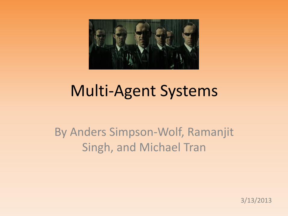
Simulation Result
-1.5 -1 -0.5 0 0.5 1 1.50
0.5
1
1.5
2
2.5
3
X: -0.8667
Y: 0.6667
X: 1.133
Y: 0.6667
X: 1.133
Y: 2.667
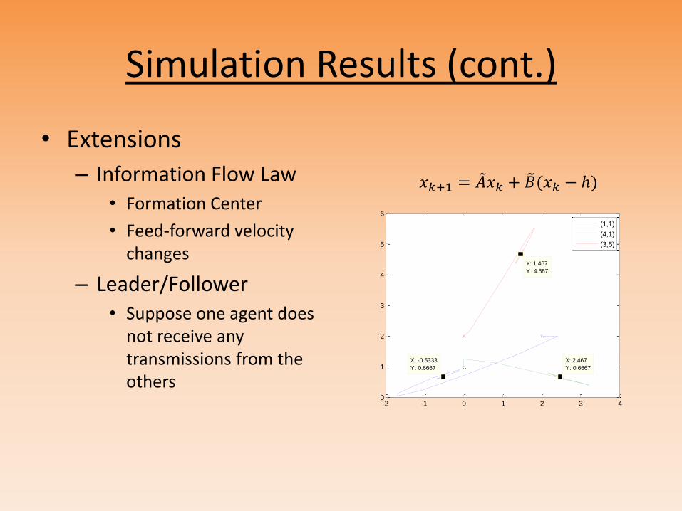
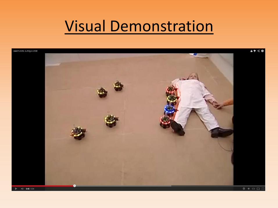
Simulation Results (cont.)
• Extensions
– Information Flow Law • Formation Center
• Feed-forward velocity changes
– Leader/Follower • Suppose one agent does
not receive any transmissions from the others
𝑥𝑘+1 = 𝐴 𝑥𝑘 + 𝐵 (𝑥𝑘 − ℎ)
-2 -1 0 1 2 3 40
1
2
3
4
5
6
X: -0.5333
Y: 0.6667
X: 1.467
Y: 4.667
X: 2.467
Y: 0.6667
(1,1)
(4,1)
(3,5)
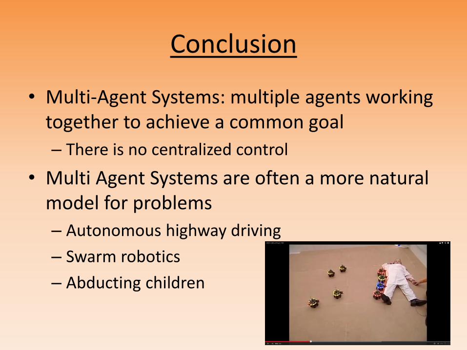
Conclusion
• Multi-Agent Systems: multiple agents working together to achieve a common goal
– There is no centralized control
• Multi Agent Systems are often a more natural model for problems
– Autonomous highway driving
– Swarm robotics
– Abducting children

The End
• Thank you for your attention
• Please direct all questions to Anders
Bibliography and Additional Resources
• http://mitpress.mit.edu/sites/default/files/titles/content/9780262731317_sch_0001.pdf
• http://www.cs.cmu.edu/~softagents/multi.html
• http://en.wikipedia.org/wiki/Multi-agent_system
• http://www.masfoundations.org/mas.pdf
• Information Flow and Cooperative Control of Vehicle Formations (IEEE Transactions on Automatic Control, Vol 49, No. 9, Sept 2004)
• http://link.springer.com/journal/volumesAndIssues/10458
• http://personal.stevens.edu/~yguo1/EE631/Lafferriere.pdf
• Graph LaPlacians and Stabilization of Vehicle Formations (in Proc. 15th IFAC Conf., 2002, pp. 283-288)
Recommended