Moving-Average Transient Model for Predicting the
Back-surface Temperature of Photovoltaic Modules
by
Matthew Prilliman
A Thesis Presented in Partial Fulfillment
of the Requirements for the Degree
Master of Science
Approved April 2020 by the
Graduate Supervisory Committee:
Govindasamy Tamizhmani, Co-Chair
Patrick Phelan, Co-Chair
Liping Wang
ARIZONA STATE UNIVERSITY
May 2020

i
ABSTRACT
The operating temperature of photovoltaic (PV) modules has a strong impact on
the expected performance of said modules in photovoltaic arrays. As the install capacity
of PV arrays grows throughout the world, improved accuracy in modeling of the expected
module temperature, particularly at finer time scales, requires improvements in the
existing photovoltaic temperature models. This thesis work details the investigation,
motivation, development, validation, and implementation of a transient photovoltaic
module temperature model based on a weighted moving-average of steady-state
temperature predictions.
This thesis work first details the literature review of steady-state and transient
models that are commonly used by PV investigators in performance modeling. Attempts
to develop models capable of accounting for the inherent transient thermal behavior of
PV modules are shown to improve on the accuracy of the steady-state models while also
significantly increasing the computational complexity and the number of input
parameters needed to perform the model calculations.
The transient thermal model development presented in this thesis begins with an
investigation of module thermal behavior performed through finite-element analysis
(FEA) in a computer-aided design (CAD) software package. This FEA was used to
discover trends in transient thermal behavior for a representative PV module in a timely
manner. The FEA simulations were based on heat transfer principles and were validated
against steady-state temperature model predictions. The dynamic thermal behavior of PV
modules was determined to be exponential, with the shape of the exponential being
dependent on the wind speed and mass per unit area of the module.

ii
The results and subsequent discussion provided in this thesis link the thermal
behavior observed in the FEA simulations to existing steady-state temperature models in
order to create an exponential weighting function. This function can perform a weighted
average of steady-state temperature predictions within 20 minutes of the time in question
to generate a module temperature prediction that accounts for the inherent thermal mass
of the module while requiring only simple input parameters. Validation of the modeling
method presented here shows performance modeling accuracy improvement of 0.58%, or
1.45°C, over performance models relying on steady-state models at narrow data intervals.

iii
DEDICATION
To,
My parents, Jeff and Michelle Prilliman, who have always supported me and pushed me
to follow my dreams.
My friends and family, who have shown me love and kindness every day of my life.
My grandfather Thomas Peltier, who always instilled in me the value of education and
was my biggest supporter. May he rest in peace.

iv
ACKNOWLEDGMENTS
I would like to offer gratitude to Dr. Govindasamy Tamizhmani for allowing me to work
and perform research in the Photovoltaic Reliability Lab (PRL) at ASU. He has been a
great mentor throughout my graduate studies and I have learned a lot from my time working
with him. Thanks must also go to the staff and students at PRL for their support and
kindness throughout my time here at ASU. I would particularly like to thank Sai Tatapudi,
Telia Curtis, Dr. Bulent Nicer, Ashwini Pavgi, and Hamsini Gopalakrishna for their
guidance and companionship.
Thank you also to my committee members, co-chair Dr. Patrick Phelan and Dr. Liping
Wang, for serving on my thesis committee.
Special thanks to the team at Sandia National Laboratories Photovoltaic System Evaluation
Laboratory (PSEL) for supporting my time here as ASU financially and for guiding my
research. Thank you to Josh Stein for your mentorship and for guiding me through this
project. Thank you also to Daniel Riley for your mentorship and patience in answering my
many questions over the years.
This material is based upon work supported by the U.S. Department of Energy’s Office of
Energy Efficiency and Renewable Energy (EERE) under Solar Energy Technologies
Office (SETO) Agreement Number 34366.
This work was funded by Sandia National Laboratories under a contract with Arizona State
University’s Photovoltaic Reliability Laboratory (PRL).

v
TABLE OF CONTENTS
Page
LIST OF TABLES ................................................................................................................. vii
LIST OF FIGURES .............................................................................................................. viii
CHAPTER
1 INTRODUCTION ................................................................................................ 1
1.1 Background.................................................................................................. 1
1.2 Problem Statement ...................................................................................... 2
1.3 Scope of the Work ....................................................................................... 3
2 LITERATURE REVIEW ..................................................................................... 5
2.1 Temperature Dependence of PV Modules ................................................. 5
2.2 Steady-state Thermal Models ..................................................................... 6
2.3 RC Circuit Dynamic Thermal Models ..................................................... 11
2.4 Transient Thermal Models ........................................................................ 12
2.5 Importance of Transient Thermal Modeling ............................................ 16
3 METHODOLOGY ............................................................................................... 18
3.1 FEA Modeling Approach .......................................................................... 18
3.2 Heat Transfer Definitions .......................................................................... 22
3.2.1 Convection ........................................................................................ 23
3.2.2 Radiation ........................................................................................... 25
3.2.3 Conduction ........................................................................................ 27
3.2.4 Irradiance .......................................................................................... 27
3.2.5 Transient Considerations .................................................................. 28

vi
CHAPTER PAGE
3.3 FEA Model Validation .............................................................................. 28
3.4 Transient FEA Simulation Methodology and Results ............................. 30
3.5 Moving-Average Model Development ..................................................... 45
3.6 Moving-Average Model Implementation ................................................. 54
4 RESULTS AND DISCUSSIONS ........................................................................ 61
4.1 Data Handling ............................................................................................ 61
4.2 Data Filtering ............................................................................................. 62
4.3 Cumulative Distribution Function Analysis ............................................. 66
4.4 Moving-Average Model Fit to Measured Data ........................................ 69
4.5 Comparison of Different Module Types .................................................. 81
4.6 Histogram Analysis ................................................................................... 86
4.7 Significance of the Work .......................................................................... 88
5 CONCLUSIONS .................................................................................................. 90
5.1 Future Work............................................................................................... 91
REFERENCES ...................................................................................................................... 93
APPENDIX
A MOVING-AVERAGE MODEL OPEN-SOURCE CODE .................................... 97
B MODEL VALIDATION SOURCE CODE ........................................................... 101

vii
LIST OF TABLES
Table Page
1. Sandia Array Performance Model Coefficients ........................................................... 7
2. Steady-state FEA Simulated Module Back-Surface Temperature Residual Comparison
to Steady-State Model .................................................................................................. 30
3. Bilinear Interpolation Coefficients for Exponential Weighting Factor ...................... 54
4. Moving-Average Model Example Calculation ........................................................... 58
5. Fit Statistics for Moving-Average Model and Steady-State Model for Different
Climates ........................................................................................................................ 71
6. Fit Statistics for Moving-Average Model and Default Steady-State Models for Different
Climates ........................................................................................................................ 75
7. Comparison of Glass-Backsheet and Glass-Glass Module Temperatures Fit to Moving-
Average Model ............................................................................................................. 83
8. Improvement in PV Performance Modeling Accuracy for Thermal Accuracy
Improvements of Moving-Average Model .................................................................. 89
viii
LIST OF FIGURES
Figure Page
1. RC Circuit Representation of the Thermal Resistance and Capacitance of PV Module
Layers ........................................................................................................................... 11
2. Optimized Transient Thermal Model Accuracy Improvements over Steady-State Model
....................................................................................................................................... 13
3. Transient Thermal Model Accuracy Improvement over Steady-State Model for Different
Climates ....................................................................................................................... 14
4. Shading Test with Measured and Modeled Module Temperatures ............................. 19
5. FEA Simulation Process Diagram ................................................................................ 21
6. Simulation Heat Transfer Diagram .............................................................................. 23
7. Irradiance Step Change Sizes for FEA Simulations .................................................... 31
8. FEA Decreasing Temperature Simulations for Spring ................................................ 32
9. FEA Decreasing Temperature Simulations for Summer ............................................. 33
10. FEA Decreasing Temperature Simulations for Winter ............................................. 34
11. FEA Simulated Temperatures for Different Unit Masses ......................................... 36
12. Temperature Stabilization Time for Wind Speed and Unit Mass ............................. 38
13. Irradiance Step Change Sizes for Increasing Temperature Simulations ................... 39
14. FEA Increasing Temperature Simulations for Spring ............................................... 40
15. FEA Increasing Temperature Simulations for Summer ............................................ 41
16. FEA Increasing Temperature Simulations for Winter ............................................... 42
17. Temperature Stabilization Time for Increasing Temperature Simulations ............... 44
ix
Figure Page
18. Steady-state Temperature Prediction Inaccuracy as Compared to FEA Transient
Simulation Module Temperatures ............................................................................... 47
19. Fit of Exponentially Weighted Steady-State Temperature Predictions to FEA Simulated
Temperatures ................................................................................................................ 49
20. Illustration of Exponential Thermal Ramp Rate of PV Module Temperature .......... 50
21. Power Parameter as a Function of Wind Speed and Unit Mass ................................ 51
22. Planar fit of Exponential Weighting Factor to Wind Speed and Module Unit Mass 53
23. Empirical CDF Analysis of Moving-Average Model Fit to Albuquerque Data ....... 68
24. Summer Example of Moving-Average Model Fit to Measured Data
(Albuquerque) ............................................................................................................. 73
25. Winter Example of Moving-Average Model Fit to Measured Data
(Albuquerque) ............................................................................................................. 74
26. Default Steady-State Moving-Average Model Implementation for a Summer Day 76
27. Default Steady-State Moving-Average Model Implementation for a Winter Day ... 77
28. Monthly RMSE for Moving-Average and Steady-State Models (Albuquerque) ..... 78
29. Monthly RMSE for Moving-Average and Steady-State Models (Orlando) ............. 79
30. Monthly RMSE for Moving-Average and Steady-State Models (Las Vegas) ......... 80
31. Monthly RMSE for Moving-Average and Steady-State Models (Vermont) ............ 81
32. Glass-Glass Module Behavior for Incorrect Unit Mass in Summer ......................... 85
33. Glass-Glass Module Behavior for Correct Unit Mass in Summer ............................ 85
34. Histogram Analysis for Albuquerque Model Fit ....................................................... 87
35. Histogram Analysis for Orlando Model Fit ............................................................... 87

x
Figure Page
36. Histogram Analysis for Las Vegas Model Fit ........................................................... 87
37. Histogram Analysis for Vermont Model Fit .............................................................. 88

1
CHAPTER 1
INTRODUCTION
1.1 Background
The performance of PV modules is dependent on many factors that must each be
accounted for when modeling the expected performance of said modules over a given
period. Accurate prediction of the operating temperature of PV modules is second only to
irradiance in terms of importance to accurate PV performance modeling [1]. The power
performance of PV modules can be expected to decrease by a factor of 0.3 - 0.5 %/°C
increase in temperature above the rated module temperature as a result of decreased cell
voltage output [1]. The module temperature varies over time as a function of irradiance
hitting the module’s front and rear surfaces, convection due to wind flow and still air,
heat radiation to the module’s surroundings and the atmosphere, heat conduction through
the different layers of the module, and power production in the form of electrical energy
that reduces the amount of energy within the module that is dissipated as heat. As such,
accurately predicting the temperature that a photovoltaic module operates at in a given
moment requires accounting for many environmental parameters, material properties, and
electrical considerations.
The impact that module temperature has on PV performance makes accurate modeling of
PV temperature essential to understanding the expected performance of the modules.
Predicting the expected performance of a PV array is an essential part of the planning
phase that investors and project managers go through when developing new PV projects.
While this predictive modeling is currently done on a predominately hourly basis,
budding interest in different inverter technologies and energy storage capabilities make

2
temperature modeling at sub-hourly timesteps a point of interest within the industry [2],
[3]. Accuracy in module temperature forecasting also plays an essential role in
troubleshooting incorrect temperature readings from the PV array field or unsafe module
operating conditions resulting from overheating.
The current best practices in PV temperature modeling involve the use of validated
steady-state temperature models based on the irradiance, wind speed, and ambient
temperature data for a given PV array site [4]–[9]. Additionally, steady-state models
based on rated module temperatures found from test procedures described in international
test standards are used as a basis for steady-state modeling of back-surface temperature
[10]. Attempts at transient models designed to account for a module’s inherent thermal
mass due to the module materials’ thermal properties have offered increased accuracy at
the expense of increased computational complexity that leads to resistance from industry
[11]–[14]. The accuracy improvements of these published transient thermal models are
significant enough to warrant consideration from the PV modeling industry, but the
numerous input parameters that must be found to effectively run the model for a given
site cause resistance from industry in applying the model into their performance modeling
practices. There is an industry-wide need for an accurate temperature model that accounts
for the material considerations affecting heat transfer and is based on only a few input
parameters.
1.2 Problem Statement
As the interest in accurate modeling of PV performance at finer time scales increases, the
need for more accurate modeling of module temperature on a transient basis also
increases. The model developed to meet this industry-wide need must account for the
3
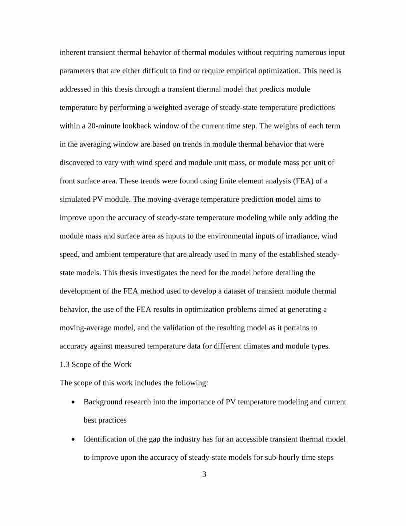
inherent transient thermal behavior of thermal modules without requiring numerous input
parameters that are either difficult to find or require empirical optimization. This need is
addressed in this thesis through a transient thermal model that predicts module
temperature by performing a weighted average of steady-state temperature predictions
within a 20-minute lookback window of the current time step. The weights of each term
in the averaging window are based on trends in module thermal behavior that were
discovered to vary with wind speed and module unit mass, or module mass per unit of
front surface area. These trends were found using finite element analysis (FEA) of a
simulated PV module. The moving-average temperature prediction model aims to
improve upon the accuracy of steady-state temperature modeling while only adding the
module mass and surface area as inputs to the environmental inputs of irradiance, wind
speed, and ambient temperature that are already used in many of the established steady-
state models. This thesis investigates the need for the model before detailing the
development of the FEA method used to develop a dataset of transient module thermal
behavior, the use of the FEA results in optimization problems aimed at generating a
moving-average model, and the validation of the resulting model as it pertains to
accuracy against measured temperature data for different climates and module types.
1.3 Scope of the Work
The scope of this work includes the following:
• Background research into the importance of PV temperature modeling and current
best practices
• Identification of the gap the industry has for an accessible transient thermal model
to improve upon the accuracy of steady-state models for sub-hourly time steps

4
• Examination of the expected thermal behavior for a generalized construction of a
PV module under a variety of different environmental operating conditions
through finite element analysis (FEA) methods
• Fitting of the steady-state temperature predictions for the environmental
conditions applied in the FEA simulations to the FEA simulated temperatures
through an exponentially weighted moving-average of the steady-state predictions
within a fixed time lookback window
• Development of the final moving-average model equation based on bilinear
interpolation of the optimized weighting function coefficients with the wind speed
and unit mass conditions that resulted in said coefficients
• Example use of the module for real PV array data to demonstrate the model
calculations for a given time step
• Validation of the moving-average model in terms of the accuracy improvements
over the steady-state model and previously published transient models
• Validation of the moving-average model in terms of the reduced variability in
temperature prediction for sub-hourly time intervals in comparison to steady-state
models
• Reflections on the validation results and what they mean to the PV industry at-
large
• Recommendations on future work to further improve the PV temperature
modeling practices used in industrial and research laboratory settings

5
CHAPTER 2
LITERATURE REVIEW
The dependence of PV performance on module temperature has led to a vast amount of
peer-reviewed publications on the modeling and monitoring of PV module temperatures.
The majority of this research has been based on steady-state calculations of the module
temperature that use the plane-of-array (POA) irradiance, wind speed, and ambient
temperature of the array site in the calculation. Some of these models have been used in
PV modeling practices for decades, as they have been proven accurate for the hourly time
steps that are often used in PV modeling. Despite the large amount of research in PV
temperature modeling that is present, there has not been much research into transient
thermal modeling of PV modules to model the thermal behavior at more narrow data
intervals. The transient models that have been published have not been readily accepted
into the thermal modeling practices of the majority of the PV industry. Industry resistance
can be attributed to the fact that these transient models require many input parameters
that are difficult to obtain or measure. The large number of variables has also led these
models to be complex in computation, which has also led to industry resistance.
2.1 Temperature dependence of PV performance
There have been numerous studies showing that the power output of PV arrays decreases
for increases in temperature beyond the rated temperature of the modules. The degree to
which the PV performance is expected to decrease ranges between 0.3-0.5%/°C of the
rated maximum power point depending on the module materials and manufacturing
methods [1]. The decrease in power from the PV modules for increasing temperature is
based on decreased voltage from the cells due to a reduced band gap [15]. Compared to

6
the voltage, the current produced in the photovoltaic conversion process has a negligible
relationship with operating temperature, increasing only slightly for increasing
temperature [15]. As the maximum power point of a module is dependent on the open-
circuit voltage and short-circuit current, the power decreases as a result of increasing
temperature beyond the rated temperature [15], [16]. This relationship shows that
accurate prediction of the temperature is essential to accurately predicting PV
performance, and that the area of PV temperature modeling must be researched and
improved upon as PV technologies increase in global capacity.
2.2 Steady-state Temperature modeling
Temperature models used to predict the operating temperature of PV modules have been
mostly based on steady-state approximations that take environmental parameters as
inputs. These steady-state models are based on measured variables such as the solar
irradiance incident on the module, the surrounding ambient temperature at the site in
which the PV array is installed, the wind speed at the site, and in some cases the wind
direction relative to the module [4]–[9], [17]. Evaluating the temperature of the module
based on these parameters allows for reasonably accurate hourly temperature predictions
without requiring knowledge of the PV array power performance. These temperature
models are often deployed as part of an overall PV performance evaluation to evaluate
the annual energy performance of a PV array.
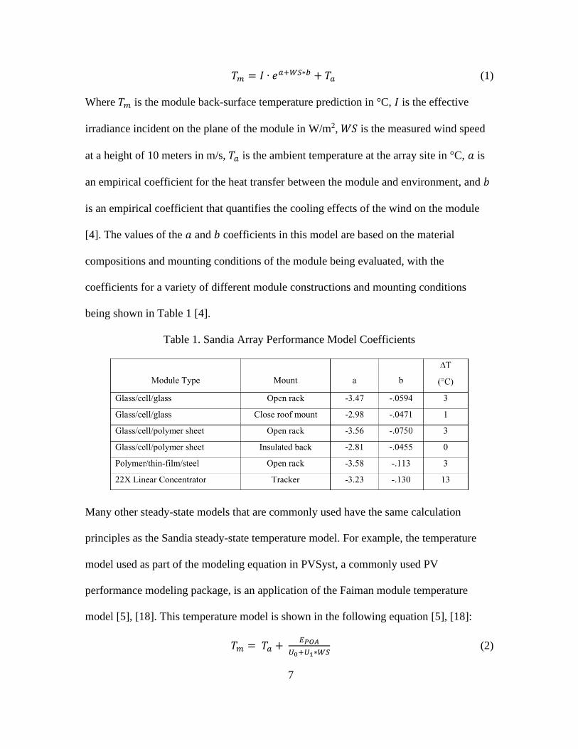
One commonly used steady-state model is the one put forth in the Sandia Array
Performance Model [4]. This model was developed through empirical optimization of
measured module temperature data and was proven to be accurate to within 5°C of
measured data [4]. The model equation is shown below [4]:
7
𝑇𝑚 = 𝐼 ∙ 𝑒𝑎+𝑊𝑆∗𝑏 + 𝑇𝑎 (1)
Where 𝑇𝑚 is the module back-surface temperature prediction in °C, 𝐼 is the effective
irradiance incident on the plane of the module in W/m2, 𝑊𝑆 is the measured wind speed
at a height of 10 meters in m/s, 𝑇𝑎 is the ambient temperature at the array site in °C, 𝑎 is
an empirical coefficient for the heat transfer between the module and environment, and 𝑏
is an empirical coefficient that quantifies the cooling effects of the wind on the module
[4]. The values of the 𝑎 and 𝑏 coefficients in this model are based on the material
compositions and mounting conditions of the module being evaluated, with the
coefficients for a variety of different module constructions and mounting conditions
being shown in Table 1 [4].
Table 1. Sandia Array Performance Model Coefficients
Many other steady-state models that are commonly used have the same calculation
principles as the Sandia steady-state temperature model. For example, the temperature
model used as part of the modeling equation in PVSyst, a commonly used PV
performance modeling package, is an application of the Faiman module temperature
model [5], [18]. This temperature model is shown in the following equation [5], [18]:
𝑇𝑚 = 𝑇𝑎 + 𝐸𝑃𝑂𝐴
𝑈0+𝑈1∗𝑊𝑆 (2)
8
Where 𝑇𝑚 is the module temperature in °C, 𝑇𝑎 is the ambient temperature in °C, 𝐸𝑃𝑂𝐴 is
the incident irradiance in W/m2, 𝑈0 and 𝑈1 are empirical heat transfer coefficients, and
𝑊𝑆 is the wind speed in m/s. Simple derivations would show that this model is of the
same form as the Sandia steady-state model [5], [18], [19].
The steady-state models shown in (1) and (2) are used to predict the temperature of the
module’s back surface rather than the temperature of the actual PV cells contained within
the glass, encapsulant, and backsheet layers of the module. The back-surface temperature
is often calculated instead of the cell temperature in order to relate the temperature to the
site’s wind speed, as the wind is directly hitting the exposed surfaces of the module and is
not directly interfacing with the PV cells. Additionally, measuring the back-surface
temperature in the PV array field is a much less invasive practice than measuring the cell
temperature directly, as doing so requires adhering a temperature measurement device to
the cell during module construction. It is often necessary to convert these back-surface
temperature calculations to the cell temperature, as the temperature of the cell is what
ultimately determines the electrical output of the cells based on the previously defined
temperature dependence. To correlate the back-surface temperature predictions to cell
temperature predictions, the Sandia Array Performance Model uses a linear relation in
which the ratio of the incident irradiance to an assumed reference irradiance value of
1000 W/m2 is multiplied by an temperature differential constant that was determined
empirically for different module constructions and mounting conditions [4]. The product
of this calculation is added to the back-surface temperature prediction to determine the
cell temperature. The calculation of the cell temperature based on the Sandia steady-state
model module temperature is shown below [4]:

9
𝑇𝑐 = 𝑇𝑚 + 𝐸𝑃𝑂𝐴
𝐸0Δ𝑇 (3)
Where 𝑇𝑐 is the cell temperature in °C, 𝐸0 is the reference irradiance of 1000 W/m2 and
Δ𝑇 is the empirical temperature differential constant. The temperature differential
constants Δ𝑇 are shown in the rightmost column of Table 1 [4].
The PVSyst method of converting Faiman model module temperature predictions to cell
temperature predictions involves adjusting irradiance as a function of the cell efficiency
and the optical properties of the glass and cells [5], [18]. The PVSyst cell temperature
model is described by the following equation [18]:
𝑇𝑐 = 𝑇𝑎 + 𝐸𝑃𝑂𝐴𝛼(1−𝑒𝑡𝑎𝑚)
𝑈0+𝑈1∗𝑊𝑆 (4)
Where 𝑇𝑐 is the cell temperature in °C, 𝛼 is the absorptance of the cells, and 𝑒𝑡𝑎𝑚 is the
solar cell efficiency [18].
Other methods of calculating PV cell temperatures make use of the Nominal Operating
Cell Temperature (NOCT) or Nominal Module Operating Temperature (NMOT), which
are reference operating temperatures for modules that are found through test procedures
and modeling defined by the International Electrotechnical Commission (IEC) 61215
standard [20]. NMOT is an updated version of the NOCT, and many PV manufacturers
perform or outsource the test as specified in the standard to then report one of these
nominal temperature values in their module spec sheets. The NMOT defines the expected
temperature of the module at reference conditions of 800 W/m2, 1 m/s wind speed, and
20°C ambient temperature over a data measurement period spanning several days [20],
[21]. Finding the module temperature at these exact ambient conditions requires
collecting large amounts of data in stable environmental conditions before fitting the
10
dataset linearly in order to then interpolate to the standard conditions set in the standard.
Once this NMOT or NOCT is found, the temperature predictions for the module can be
found from equations such as the following proposed in Duffie and Beckman [10]:
𝑇𝐶 − 𝑇𝑎
𝑇𝑁𝑂𝐶𝑇− 𝑇𝑎,𝑁𝑂𝐶𝑇 =
𝐺𝑇
𝐺𝑁𝑂𝐶𝑇∗
9.5
(5.7+3.8∗𝑉)(1 −
𝜂𝐶
𝜏𝛼) (5)
Where 𝑇𝐶 is the cell temperature, 𝑇𝑎 is the ambient temperature, 𝑇𝑁𝑂𝐶𝑇 is the rated NOCT
of the module, 𝑇𝑎,𝑁𝑂𝐶𝑇 is the ambient temperature of the NOCT which is set constant at
20°C, 𝐺𝑇 is the irradiance incident on the module, 𝐺𝑁𝑂𝐶𝑇 is the irradiance of the NOCT
test of 800 W/m2, 𝑉 is the wind speed, 𝜂𝐶 is the cell electrical conversion efficiency, and
𝜏𝛼 is the product of the transmittance of the glass and absorptance of the cells [10].
Steady-state models such as the Sandia steady-state thermal model described in preceding
paragraphs have been proven to be accurate within 5°C for most stable climate conditions
considered over large data intervals such as hourly data [4]. However, as previous work
has shown that PV performance modeling errors can be reduced by evaluating
performance at narrower data intervals [22], there is an interest in accurately modeling
PV module temperature based on more instantaneous changes in incident irradiance or
other environmental variables. Under such conditions, the direct relationship between
module temperature and irradiance in these steady-state models can lead to large spikes
in module temperature for step changes in incident irradiance. This predicted thermal
behavior is not always an accurate depiction of module thermal behavior, as PV modules
have thermal mass that slows the rate of temperature change to changes in the
environment. As these models do not account for the inherent thermal mass of the
module materials, some research into modeling the dynamic, or transient, thermal
response of PV modules for environmental changes has been performed and published.

11
2.3 RC Circuit dynamic thermal models
One commonly used approach to modeling the dynamic thermal response of PV modules
is to use a resistance-capacitance (RC) circuit as an analogy to calculate said thermal
behavior. The RC circuit analogy allows for consideration of the thermal resistance and
capacitance of each individual module layer [23], [24]. The thermal resistances of each
layer are treated as resistive elements operating in series, with each element’s thermal
resistance being based on the material thickness and thermal conductivity of the material.
The thermal capacitances operate in parallel and are based on material density, thickness,
and heat capacity [23], [24]. An example of such an RC circuit is shown in Figure 1 [23].
Treating the model thermal behavior as a circuit allows for the calculation of thermal
time constants that signify the amount of time needed for a module to heat or cool to a
given temperature or percentage of thermal stabilization [23], [24]. Implementing this
circuit analogy for transient thermal analysis of PV modules requires that all the thermal
properties of each module layer be accurately measured. As these material properties can
be difficult to measure and may change in response to changing temperatures or
degradation, there is resistance in the PV industry to apply these practices in performance
modeling software packages.
Figure 1. RC Circuit Representation of the Thermal Resistance and Capacitance of PV
Module Layers

12
2.4 Transient Thermal Models
There have been a few transient models presented in literature as a means of more
accurately predicting the instantaneous temperature of PV modules. Jones and
Underwood developed a model that performed a full energy balance of the convection,
short-wave radiation, long-wave radiation, and power generation affecting PV modules
during operation [11]. The final equations used to calculate the module temperature in
this approach are [11]:
𝐶𝑚𝑜𝑑𝑢𝑙𝑒𝑑𝑇𝑚𝑜𝑑𝑢𝑙𝑒
𝑑𝑡= 𝜎 ∗ 𝐴 ∗ (𝜀𝑠𝑘𝑦(𝑇𝑎𝑚𝑏𝑖𝑒𝑛𝑡 − 𝜕𝑇)4 − 𝜀𝑚𝑜𝑑𝑢𝑙𝑒𝑇𝑚𝑜𝑑𝑢𝑙𝑒
4) + 𝛼 ∗ Φ ∗ 𝐴 −
𝐶𝐹𝐹∗𝐸∗ln(𝑘1𝐸)
𝑇𝑚𝑜𝑑𝑢𝑙𝑒− (ℎ𝑐,𝑓𝑜𝑟𝑐𝑒𝑑 + ℎ𝑐,𝑓𝑟𝑒𝑒) ∗ 𝐴 ∗ (𝑇𝑚𝑜𝑑𝑢𝑙𝑒 − 𝑇𝑎𝑚𝑏𝑖𝑒𝑛𝑡) (6)
𝑇𝑚𝑜𝑑𝑢𝑙𝑒(𝑡 + 1) = 𝑇𝑚𝑜𝑑𝑢𝑙𝑒(𝑡) = 𝑠𝑡𝑒𝑝 ∗ (𝑑𝑇𝑚𝑜𝑑𝑢𝑙𝑒
𝑑𝑡) (7)
Where 𝐶𝑚𝑜𝑑𝑢𝑙𝑒 is the overall capacitance of the module, 𝑑𝑇𝑚𝑜𝑑𝑢𝑙𝑒
𝑑𝑡 is the change in module
temperature with respect to time 𝑡, 𝜎 is the Stefan Boltzmann constant, 𝐴 is the surface
area of the module in square meters, 𝜀𝑠𝑘𝑦 is the emissivity of the sky, 𝜕𝑇 is a temperature
differential constant used to determine the sky temperature from the ambient temperature,
𝜀𝑚𝑜𝑑𝑢𝑙𝑒 is the emissivity of the module front surface, 𝛼 is the absorptivity of the module,
Φ is the total incident irradiance on the module front surface in W/m2, 𝐶𝐹𝐹 is the fill
factor of the module that relates the module performance to the maximum theoretical
performance, E is incident irradiance in W/m2, k1 is an empirical constant, ℎ𝑐,𝑓𝑜𝑟𝑐𝑒𝑑 is the
convection coefficient due to wind in W/m2K, and ℎ𝑐,𝑓𝑟𝑒𝑒 is the convection coefficient
due to natural convection to the surrounding air in W/m2K. This model accounts for the
total inherent thermal mass through the capacitance term on the left side of (5) and
defines the heat transfer state between the module and surrounding environment on the

13
right-hand side of the equation. The energy balance in (5) can be used to determine the
change in temperature over a given time interval, which can then be used in (6) to find
the temperature at the next time step based on the temperature at the previous time step.
When optimizing the input parameters of this model to a particular PV array site, the
predicted transient temperature predictions for 1-minute data are found to be within 2.3 K
for clear sky conditions [11]. Further analysis of the Jones and Underwood model was
done by Stein and Luketa-Hanlin, who optimized the model for a specific PV site in
Hawaii based on sensitivity studies performed on the unknown input parameters [13].
Analysis of the optimized model against measured temperature data reveals substantial
accuracy improvements over steady-state modeling for 1-second temperature data as
shown in Figure 2 [13]. Accounting for the thermal mass of the module decreases the
variability in temperature prediction and allows for more accuracy against measured
temperature data.
Figure 2. Optimized Transient Thermal Model Accuracy Improvements over Steady-
State Model
14
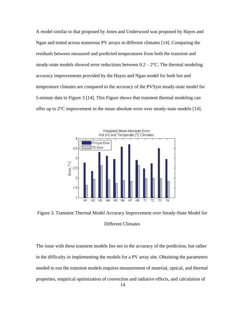
A model similar to that proposed by Jones and Underwood was proposed by Hayes and
Ngan and tested across numerous PV arrays in different climates [14]. Comparing the
residuals between measured and predicted temperatures from both the transient and
steady-state models showed error reductions between 0.2 – 2°C. The thermal modeling
accuracy improvements provided by the Hayes and Ngan model for both hot and
temperature climates are compared to the accuracy of the PVSyst steady-state model for
5-minute data in Figure 3 [14]. This Figure shows that transient thermal modeling can
offer up to 2°C improvement in the mean absolute error over steady-state models [14].
Figure 3. Transient Thermal Model Accuracy Improvement over Steady-State Model for
Different Climates
The issue with these transient models lies not in the accuracy of the prediction, but rather
in the difficulty in implementing the models for a PV array site. Obtaining the parameters
needed to run the transient models requires measurement of material, optical, and thermal
properties, empirical optimization of convection and radiative effects, and calculation of
15
values for those parameters that cannot be measured accurately. The difficulty in
accurately parametrizing these models leads to industry pushback on the adoption of
transient thermal models in their modeling practices as they relate to overall PV
performance modeling. There remains a gap in the PV industry for a thermal model that
matches or exceeds the modeling accuracy of those transient thermal models while using
a small number of easily definable input parameters. These input parameters should be
easy to measure or readily available in reported module spec sheet data.
2.5 Importance of Transient Thermal Modeling
Dynamic modeling of PV module temperature plays an important role in several different
aspects of PV performance modeling and monitoring. Failing to account for the thermal
mass of the module on a minute-to-minute basis can lead to overestimation of PV
performance at low irradiance conditions [25]. Steady-state models predict low
temperatures during times of low irradiance as they do not account for the thermal mass
of the module that slows the rate of temperature change in modules for instantaneous
changes in the incident irradiance. Similarly, using hourly average data in performance
models can lead to inaccuracies in inverter clipping models. As inverters have a
maximum voltage limit, DC voltage production of modules beyond the limit is cut off
[2], [25]. Hourly averages have been shown to underestimate the amount of module
clipping for a variety of inverter types and amounts of power output when compared to
the same analysis performed for 1-minute data [2]. These issues show that there is a need
for PV performance modeling at finer time scale. As steady-state models can provide
inaccurate predictions of module temperature at this time scale, transient thermal models
that can be easily implemented are needed.

16
Finer time steps in PV performance modeling are also needed to accurately model energy
storage systems used to make renewable energy systems dispatchable. As solar energy is
an intermittent resource that does not allow for energy production during nighttime or
cloudy conditions, the energy that is produced during times of high irradiance must often
be stored using technologies such as batteries or thermal storage in order to conserve
electrical energy produced by PV arrays to meet energy demands during periods of low
solar resource. Attempts at modeling battery storage to make PV energy production more
dispatchable have been shown to require modeling intervals no larger than 15 seconds to
provide the accuracy needed to accurately model this battery storage [3]. This again
exemplifies the need for finer temporal resolution in PV performance modeling, which
necessitates dynamic thermal modeling.
Accuracy in thermal modeling is not only crucial to performance modeling. It can also
play an integral role in the performance rating of modules before they are put on the
market. Currently, modules are rated for their temperature performance based on NMOT.
The methods used to determine these modules’ NMOT values are outlined in the IEC
61215-2 standard [20]. However, work done at the National Renewable Energy
Laboratory (NREL) has shown the data collection practices used to determine this
reported temperature value offer highly variable results for the same types of modules in
different climate conditions [21]. The NOCT values in this study were found to vary by
as much as 7°C for the same module [21]. More accuracy in thermal modeling without
increased complexity could benefit efforts to refine this standard for more accuracy and
reduced variability in module temperature rating practices. A transient model with a

17
small amount of input parameters would address this need and lead to more efficiency
and repeatability in module temperature rating.

18
CHAPTER 3
METHODOLOGY
3.1 FEA Modeling Approach
The development of the FEA simulations of module thermal behavior was aimed at
discovering trends in this behavior to aid in the development of a transient thermal model
based on only a few accessible input parameters. Using FEA for this model development
was based on the idea of modeling practices that would be accessible to the PV industry.
While heat transfer definition used in the simulations were developed without outside
influence, the idea behind using FEA as a PV thermal analysis tool has been previously
shown in [26].
The need for simulations designed to develop a dataset of module transient thermal
behavior was determined through simple module shading tests. These shading tests were
part of initial research designed to determine simpler methods of modeling transient
module thermal behavior that was performed in the summer of 2018 at the Photovoltaic
Systems Evaluation Laboratory of Sandia National Laboratories in Albuquerque, NM. A
white foam core board was used to shade a 60-cell PV module with a polymer backsheet
and aluminum frame that was operating under open-circuit condition (e.g. no electrical
load). While the foam core could not be assumed to block out 100% of the incident
irradiance, a reference cell irradiance measurement device was also shaded with the
module in order to have a measurement of the amount of irradiance being transmitted
through the foam core shade. The shade was also applied with a small air gap between
the shade and module front surface to allow for air flow cooling across the front surface.
The module temperature was allowed to stabilize during days in which there was little
19
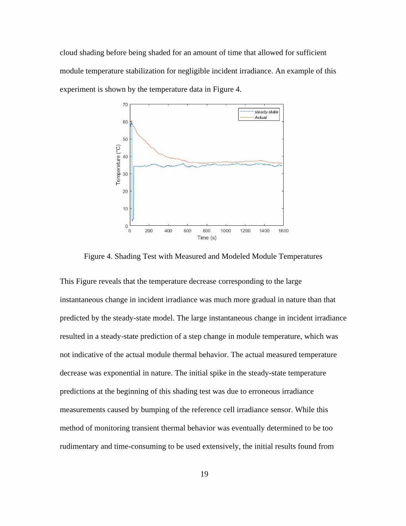
cloud shading before being shaded for an amount of time that allowed for sufficient
module temperature stabilization for negligible incident irradiance. An example of this
experiment is shown by the temperature data in Figure 4.
Figure 4. Shading Test with Measured and Modeled Module Temperatures
This Figure reveals that the temperature decrease corresponding to the large
instantaneous change in incident irradiance was much more gradual in nature than that
predicted by the steady-state model. The large instantaneous change in incident irradiance
resulted in a steady-state prediction of a step change in module temperature, which was
not indicative of the actual module thermal behavior. The actual measured temperature
decrease was exponential in nature. The initial spike in the steady-state temperature
predictions at the beginning of this shading test was due to erroneous irradiance
measurements caused by bumping of the reference cell irradiance sensor. While this
method of monitoring transient thermal behavior was eventually determined to be too
rudimentary and time-consuming to be used extensively, the initial results found from

20
this experiment led to brainstorming future research through computer simulation
methods such as FEA.
FEA software was chosen for the analysis of thermal trends instead of indoor simulations,
outdoor measurements, and computational flow dynamics (CFD). Indoor simulators offer
a truly controlled environment in which the irradiance and ambient conditions are known
more exactly, but such simulators are expensive, would require special considerations for
the incorporation of air flow into the experiment, and are not accessible to the majority
of the PV industry that would be interested in these thermal modeling efforts. Outdoor
simulations with measurements of the environmental and module temperature conditions,
such as the shading test shown in Figure 4, offer more accessibility, but less control over
the ambient temperature, wind speed, and irradiance conditions that the model is
experiencing over a given time period. This lack of control increases the measurement
time needed to develop a database of module temperature predictions encompassing a
wide range of irradiance and ambient conditions over extended time periods. CFD
analysis offers the control of indoor simulations, the data quantity of outdoor
measurements, and more increased computational complexity than FEA analysis, but was
deemed too computationally expensive and inaccessible to industry to be helpful in the
advancement of PV thermal modeling. The added information regarding the wind flow
over the modules that would be provided by CFD analysis was deemed excess to
requirements for this analysis. This choice of FEA over CFD analysis could be further
investigated in future PV thermal modeling efforts.
The FEA simulations were designed using the Solidworks Simulation FEA package of
thermal analysis tools. This software allows for the definition of thermal analyses based

21
on both steady-state and transient simulations in which thermal loads are defined by the
user as time-dependent or temperature-dependent values [27]. These software capabilities
were utilized through initial validation of the thermal modeling approach against
validated module temperature predictions in steady-state convergence simulations. Once
these steady-state convergence tests were validated against steady-state temperature
predictions, hour-long time series tests were evaluated at 30-second intervals to observe
thermal trends in module temperature for different environmental conditions. The
workflow of the FEA simulation process is shown in Figure 5.
Figure 5. FEA Simulation Process Diagram
Heat Transfer Analysis
Steady-state convergence against predicted temperatures
Transient simulations
Develop Moving-Average model from simulation trends

22
3.2 Heat Transfer Definitions
The thermal modeling of PV modules applied in the FEA simulations must be
sufficiently robust to eliminate the need for parameterization of each of the heat transfer
components in the eventual transient thermal model. This need for a robust model led to
FEA investigation of the heat transfer due to irradiance, wind convection, still air
convection, conduction, long-wave radiation, and thermal losses from the module due to
electricity generation. These heat transfer components were modeled based on how they
impacted a sheet of solid glass, which was assumed to make up most of the module
thickness for cases in which there is no metallic frame. This simplifying assumption was
made to reduce the complexity of the FEA model in order to make it more accessible to
the PV industry. The representative glass sheet was oriented at an angle of 37° relative to
the horizontal ground that was given the material properties of concrete. The bottom of
the module was set at a height of 0.6 meter above the concrete surface. The heat transfer
definitions used in the FEA simulations for the PV modules are described in the
following subsections. A diagram of the various heat transfer elements that must be
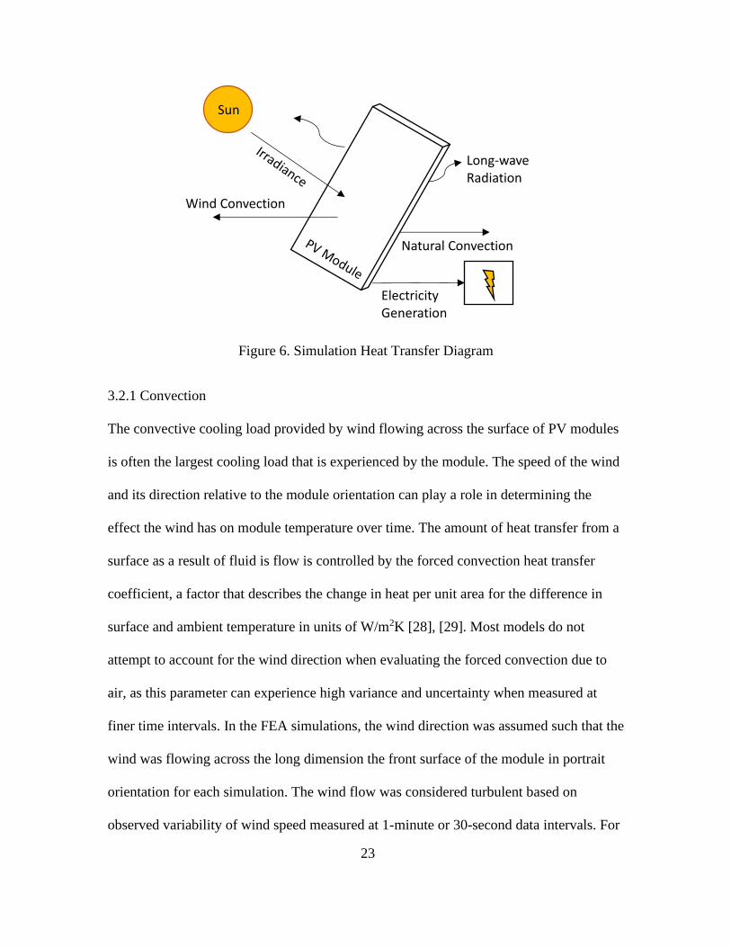
considered in the FEA simulations of the PV module is shown in Figure 6.
23
Figure 6. Simulation Heat Transfer Diagram
3.2.1 Convection
The convective cooling load provided by wind flowing across the surface of PV modules
is often the largest cooling load that is experienced by the module. The speed of the wind
and its direction relative to the module orientation can play a role in determining the
effect the wind has on module temperature over time. The amount of heat transfer from a
surface as a result of fluid is flow is controlled by the forced convection heat transfer
coefficient, a factor that describes the change in heat per unit area for the difference in
surface and ambient temperature in units of W/m2K [28], [29]. Most models do not
attempt to account for the wind direction when evaluating the forced convection due to
air, as this parameter can experience high variance and uncertainty when measured at
finer time intervals. In the FEA simulations, the wind direction was assumed such that the
wind was flowing across the long dimension the front surface of the module in portrait
orientation for each simulation. The wind flow was considered turbulent based on
observed variability of wind speed measured at 1-minute or 30-second data intervals. For
Wind Convection
Natural Convection
Long-wave Radiation
Electricity Generation
Sun

24
the FEA model, the flat plate nature of the PV module allowed for the calculation of the
heat transfer coefficient based on equations presented in Holman [29]:
𝑁𝑢 = 0.0308 𝑅𝑒4
5 𝑃𝑟1
3 (8)
ℎ =𝑁𝑢(𝑘)
𝐿 (9)
Where 𝑁𝑢 is the dimensionless Nusselt number, 𝑅𝑒 is the Reynolds number, 𝑃𝑟 is the
Prandtl number, ℎ is the convective heat transfer coefficient in W/m2K, 𝑘 is the thermal
conductivity of the air surrounding the module in W/m*K, and 𝐿 is the characteristic
length of the module in meters [29]. The Reynolds number 𝑅𝑒 is a function of the wind
speed and kinematic viscosity of the air, which was found from thermodynamic property
tables for atmospheric air along with the thermal conductivity of the air at an initial
temperature found from Sandia steady-state temperature model calculations [4], [28]. The
Reynolds number calculation is shown below:
𝑅𝑒 = 𝑊𝑆∗𝐿
𝑣(𝑇) (10)
Where 𝑊𝑆 is the wind speed in m/s, and 𝑣(𝑇) is the kinematic viscosity of air in m2/s at
the initial temperature prediction 𝑇 (°C) [28], [29].
The forced convection due to wind is assumed to dominate the cooling load on the front
surface of the module. The convection on the rear side of the module that does not
receive direct sunlight is assumed to be dominated by still air convection by the module
surface to the surrounding environment. This assumption is based on considerations of
the many different framing conditions for PV modules that often limit the amount of
wind flow that reaches the rear side of the module. Just as with the forced convection,

25
this simplifying assumption is aimed at making the modeling approach more accessible to
the PV industry. The heat transfer coefficient due to natural convection on the back
surface of the module was found from the following empirical heat transfer equations
[28], [29]:
𝑁𝑢 = 0.17((9.8 𝑐𝑜𝑠(90−𝜃)⋅(1∕𝑇𝑓))𝐼𝐿4)
(𝑘𝑣2𝑃𝑟2) (11)
ℎ =𝑁𝑢(𝑘)
𝐿 (12)
Where 𝜃 is the angle of the module relative to the ground in degrees, 𝑇𝑓 is the film
temperature of the module back surface in Kelvin, 𝐼 is the irradiance incident on the front
side of the module in W/m2, and 𝑣 is the kinematic viscosity of the air in m2/s. The film
temperature 𝑇𝑓 is found from the average of the expected back surface temperature and
the ambient temperature. Calculations for module tilt angles 𝜃 ± 30° showed module
back-surface temperature coefficients within 6% of the convection heat transfer
coefficient calculated for the 37°C tilt angle chosen for this analysis.
3.2.2 Radiation
Another key factor in module temperature calculation is the long wave radiation that
occurs between the module and its surroundings. The module in this simulation
exchanges radiative heat with both the simulated concrete ground surface and the
surrounding sky, which has been treated as a blackbody in this analysis due to its infinite
surface area. To calculate the amount of radiation between each of these surfaces, a view
factor approach was used. View factors quantify the radiation from one surface that is
absorbed by another surface, or the percentage of the surface that can “view” another
surface. The FEA software used in this analysis automatically calculates the view factors

26
of each surface relative to the other based on the geometry of the objects in the scene.
The calculations performed by the software are of the following form [27], [29]:
𝐹𝑖𝑗 = 1
𝐴𝑗∬
cos(𝜃𝑖) cos(𝜃𝑗)
𝜋𝑅𝑖𝑗2 ⅆ𝐴𝑖 ⅆ𝐴𝑗
𝑖
𝐴1 𝐴2 (13)
𝐴𝑖𝐹𝑖𝑗 = 𝐴𝑗𝐹𝑗𝑖 (14)
Where 𝐹𝑖𝑗 is the view factor for surface 𝑖 onto surface 𝑗, 𝐴𝑗 is the surface area of surface j
in square meters, and 𝜃𝑖 is the angle between the surface normal and the line 𝑅𝑖𝑗 between
the two surfaces. Steady-state simulations of module temperature for module tilt angle 𝜃
± 30° showed module back-surface temperature conditions within 1°C of the temperature
simulated for the 37°C tilt angle chosen for this analysis. (14) shows that there is
reciprocity between view factors for corresponding surfaces. This means that the sum of
the view factors for a surface 𝑖 onto all other surfaces considered in the scene must be
equal to one [27], [29]. These view factors impact the amount of net radiation exchange
between two surfaces based on the following equation [27], [29]:
𝑄𝑟𝑎𝑑𝑖𝑎𝑡𝑖𝑜𝑛 = 𝜎(𝑇𝑖
4−𝑇𝑗4)
(1−𝜀𝑖
𝐴𝑖𝜀𝑖)+
1
𝐴𝑖𝐹𝑖𝑗+(1−
𝜀𝑗
𝐴𝑖𝜀𝑖) (15)
Where 𝑄𝑟𝑎𝑑𝑖𝑎𝑡𝑖𝑜𝑛 is the net radiation exchange between surfaces in in Watts, 𝜎 is the
Stefan Boltzmann constant of 5.67e-8 W/m2*K4, 𝑇𝑖 is the temperature of surface 𝑖 in K,
and 𝜀𝑖 is the emissivity of surface 𝑖 [27]–[29].
The surrounding environment of the PV module in the simulations is assumed to be a
blackbody at a constant sky temperature. The sky temperature is found from the
following equation from Duffie and Beckman [10]:
𝑇𝑠 = 𝑇𝑎 ∗ (0.711 + 0.0056𝑇𝑑𝑝 + 0. 000073𝑇𝑑𝑝2 + 0.013 cos(15𝑡))
1
4 (16)

27
Where 𝑇𝑠 is the sky temperature in °C, 𝑇𝑑𝑝 is the dew point temperature in °C, and 𝑡 is
the hour of the day. 𝑡 was assumed to be 12 to represent solar noon testing for these
simulations [10]. The sky temperature calculation accounts for the humidity contents of
the air in the radiative heat transfer balance [10].
3.2.3 Conduction
In addition to the convection and radiation exchanges between the module and the
environment, the FEA simulations also calculate the conductive heat transfer through the
thickness of the module surface based on the thermodynamic properties of the glass.
There is typically a small temperature difference between the module’s front and back
surface. The heat exchange between through the thickness of the glass is found through
the following equation [28]:
𝑄𝑐𝑜𝑛𝑑 =𝐴∗𝑘∗∆𝑇
𝑡 (17)
Where 𝑄𝑐𝑜𝑛𝑑 is the heat due to conduction in Watts, 𝐴 is the surface area of the module
in square meters, 𝑘 is the thermal conductivity of the glass in W/m*K, ∆𝑇 is the
temperature difference between the surfaces in °C, and 𝑡 is the glass thickness [28]. This
calculation is performed within the simulation automatically and thus does not require
manual definition. The thermal conductivity of the glass used in this analysis was 0.75
W/m*K [27].
3.2.4 Irradiance
Any incident irradiance on PV modules leads to changes in the thermal state of the
module as a result of increased temperature from the photovoltaic effect of the solar cells
that generates electricity. The literature review of steady-state models showed that most
models are primarily based on the incident irradiance. As such, the irradiance incident on
28
the module must be considered in the FEA analysis for its impact on module temperature.
This is done through the application of a uniform surface heat flux across the front
surface of the PV module. The amount of irradiance present on the module front surface
is decreased by 18% of the nominal value being tested to account for the electrical
efficiency of a PV module operating at maximum power point conditions. This
simplifying assumption is made to analyze a general case of PV operation without doing
complex electrical modeling of the PV module within the FEA software environment.
The electrical efficiency was also assumed to not vary with module temperature as it
normally would in outdoor module operation [1]. The assumption was based on an
observed temperature difference of less than 2°C from temperature-dependent electrical
efficiencies in the same time series calculations.
3.2.5 Transient Considerations
When performing transient FEA simulations, the change in module temperature over time
must be considered and not assumed to be zero as it done in steady-state calculations. The
transient simulations results in an overall heat transfer similar to the model developed by
Jones and Underwood that was discussed in the previous section [11]. These calculations
were performed in the FEA simulations for glass having a constant specific heat of 0.835
kJ/kg*K [27].
3.3 FEA Model Validation
Validation of the previously mentioned heat transfer principles and simplifying
assumptions as they are applied to the simulation of PV module temperature was
achieved through steady-state convergence testing for a range of different environmental
conditions. This means that the temperature needed to solve the energy balance provided

29
by the convective and radiative loads applied to the PV module was determined for
different irradiance, ambient temperature, wind speed, and module unit mass values. A
constant irradiance load of 1000 W/m2, or 817 W/m2 after accounting for the cell
efficiency, was applied to the front-surface of the glass module for each of these
simulations. Three different ambient temperature conditions for the simulation
environment were tested in the FEA validation: -6.7°C (20°F) for typical winter
conditions, 15.6°C (60°F) for spring conditions, and 32.2°C (90°F) for summer
conditions. For each seasonal ambient temperature, constant wind speeds ranging from 1
m/s to 10 m/s were applied as part of the forced convection cooling load on the front
surface of the module. The minimum mesh element size used in these simulations was
0.08 meters. The resulting convergence temperature for each steady-state FEA simulation
was compared to the Sandia steady-state model temperature calculated from the
irradiance, wind speed, and ambient temperature considerations used in the simulation for
the coefficients a=-3.56 and b=-0.075 for a glass/cell/polymer sheet module configuration
in an open rack mount [4].
The results of the steady-state FEA simulations, along with the Sandia steady-state model
temperature predictions that the results were compared against, are shown in Table 2.
Analysis of these results shows that all of the simulated results are with the 5 degree
uncertainty of the steady-state model [4]. The FEA simulations are particularly accurate
for the warmer ambient temperatures of the spring and summer seasons. The decrease in
modeling accuracy for colder ambient temperatures could be attributed to inaccuracies
inherent to the steady-state model or to a lack of accuracy in the heat transfer definitions
in the FEA simulations. The accuracy of these simulations, particularly at higher ambient
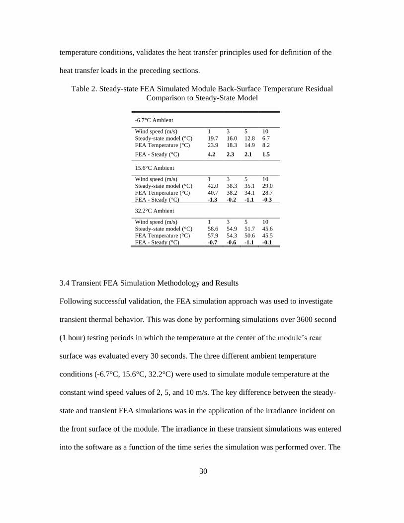
30
temperature conditions, validates the heat transfer principles used for definition of the
heat transfer loads in the preceding sections.
Table 2. Steady-state FEA Simulated Module Back-Surface Temperature Residual
Comparison to Steady-State Model
3.4 Transient FEA Simulation Methodology and Results
Following successful validation, the FEA simulation approach was used to investigate
transient thermal behavior. This was done by performing simulations over 3600 second
(1 hour) testing periods in which the temperature at the center of the module’s rear
surface was evaluated every 30 seconds. The three different ambient temperature
conditions (-6.7°C, 15.6°C, 32.2°C) were used to simulate module temperature at the
constant wind speed values of 2, 5, and 10 m/s. The key difference between the steady-
state and transient FEA simulations was in the application of the irradiance incident on
the front surface of the module. The irradiance in these transient simulations was entered
into the software as a function of the time series the simulation was performed over. The
-6.7°C Ambient
Wind speed (m/s) 1 3 5 10
Steady-state model (°C) 19.7 16.0 12.8 6.7
FEA Temperature (°C) 23.9 18.3 14.9 8.2
FEA - Steady (°C) 4.2 2.3 2.1 1.5
15.6°C Ambient
Wind speed (m/s) 1 3 5 10
Steady-state model (°C) 42.0 38.3 35.1 29.0
FEA Temperature (°C) 40.7 38.2 34.1 28.7
FEA - Steady (°C) -1.3 -0.2 -1.1 -0.3
32.2°C Ambient
Wind speed (m/s) 1 3 5 10
Steady-state model (°C) 58.6 54.9 51.7 45.6
FEA Temperature (°C) 57.9 54.3 50.6 45.5
FEA - Steady (°C) -0.7 -0.6 -1.1 -0.1

31
irradiance was set to one constant value for the first half of the simulation, then a step
change was introduced at 1800 seconds to have the irradiance either increase or decrease
to a new value that remained constant for the rest of the simulation. This step change in
irradiance allowed for analysis of the actual transient thermal behavior for large changes
in irradiance and correlation of said thermal behavior to different simulation parameters.
The initial irradiance in each test was calculated from a reference value of 1000 W/m2
that was adjusted to value of 817 W/m2 to account for the assumed cell efficiency of
18.3%. The step decrease in the irradiance was then calculated as a percentage of this 817
W/m2 initial value, with a ∆E of 600 W/m2 resulting in a final irradiance value that is
40% of the original or 326.8 W/m2. Irradiance step changes of 200, 400, and 600 W/m2
were tested for each wind speed and ambient temperature condition for a total of 18
unique FEA simulations. The irradiance step changes for these decreasing irradiance
simulations are shown graphically in Figure 7.
Figure 7. Irradiance Step Change Sizes for FEA Simulations
0
200
400
600
800
1000
1200
0 900 1800 2700 3600
Inci
den
t Ir
radia
nce
(W
/m²)
Time (seconds)
∆E = 600 W/m²
(Open Circuit)
∆E = 600 W/m²
∆E = 400 W/m²
∆E = 200 W/m²

32
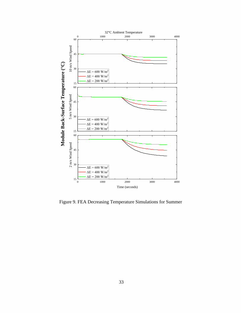
The results of the FEA transient simulations for three differently sized step decreases in
incident irradiance across three different ambient temperature conditions and three
different wind speed conditions are shown in Figures 8-10.
Figure 8. FEA Decreasing Temperature Simulations for Spring
0 1000 2000 3000 400015
30
45
60
15
30
45
60
0 1000 2000 3000 4000
15
30
45
60
2 m
/s W
ind S
pee
d
Time (seconds)
ΔE = 600 W/m2
ΔE = 400 W/m2
ΔE = 200 W/m2
16°C Ambient TemperatureM
od
ule
Back
-Su
rfa
ce T
emp
era
ture
(°C
)
5 m
/s W
ind S
pee
d
ΔE = 600 W/m2
ΔE = 400 W/m2
ΔE = 200 W/m2
10 m
/s W
ind S
pee
d
ΔE = 600 W/m2
ΔE = 400 W/m2
ΔE = 200 W/m2
33
Figure 9. FEA Decreasing Temperature Simulations for Summer
0 1000 2000 3000 4000-5
5
15
25
35
-5
5
15
25
35
0 1000 2000 3000 4000
-5
5
15
25
35
2 m
/s W
ind S
pee
d
Time (seconds)
ΔE = 600 W/m2
ΔE = 400 W/m2
ΔE = 200 W/m2
-7°C Ambient Temperature
Mod
ule
Back
-Su
rfa
ce T
emp
era
ture
(°C
)
5 m
/s W
ind S
pee
d
ΔE = 600 W/m2
ΔE = 400 W/m2
ΔE = 200 W/m2
10 m
/s W
ind S
pee
d
ΔE = 600 W/m2
ΔE = 400 W/m2
ΔE = 200 W/m2
0 1000 2000 3000 400015
30
45
60
15
30
45
60
0 1000 2000 3000 4000
15
30
45
60
2 m
/s W
ind
Sp
eed
Time (seconds)
ΔE = 600 W/m2
ΔE = 400 W/m2
ΔE = 200 W/m2
32°C Ambient Temperature
5 m
/s W
ind
Sp
eed
ΔE = 600 W/m2
ΔE = 400 W/m2
ΔE = 200 W/m2
10
m/s
Win
d S
pee
d ΔE = 600 W/m2
ΔE = 400 W/m2
ΔE = 200 W/m2

34
Figure 10. FEA Decreasing Temperature Simulations for Winter
Initial analysis of these Figures shows that the temperature decrease from the initial
stabilized module back-surface temperature to the final temperature is exponential in
nature. The size of the decrease in irradiance from the initial value has a clear effect on
the final stabilized temperature of the module’s back-surface (i.e. the temperature at the
final time step), with a greater decrease in irradiance corresponding to lower simulated
0 1000 2000 3000 4000-5
5
15
25
35
-5
5
15
25
35
0 1000 2000 3000 4000
-5
5
15
25
35
2 m
/s W
ind S
pee
d
Time (seconds)
ΔE = 600 W/m2
ΔE = 400 W/m2
ΔE = 200 W/m2
-7°C Ambient Temperature
Mod
ule
Back
-Su
rfa
ce T
emp
era
ture
(°C
)
5 m
/s W
ind S
pee
d
ΔE = 600 W/m2
ΔE = 400 W/m2
ΔE = 200 W/m2
10 m
/s W
ind S
pee
d
ΔE = 600 W/m2
ΔE = 400 W/m2
ΔE = 200 W/m2

35
module back-surface temperatures for constant wind speed and ambient temperature
conditions.
Further analysis of the individual FEA simulations shows that for increasing wind speed,
the slope of the exponential temperature curve is flattened across all ambient temperature
conditions due to the increased wind cooling load reducing the amount of time needed for
temperature stabilization. Visual comparisons across the different ambient temperature
conditions in each Figure reveal that the ambient temperature changes the initial
stabilization temperature but does not dramatically impact the rate of temperature
decrease for identical wind speed conditions. These observations reveal that wind speed
is an important parameter when considering the transient thermal behavior in PV modules
as it changes the slope of the exponential thermal decay. It also shows that ambient
temperature, a primary input to existing steady-state thermal models, is not particularly
useful in determining the transient thermal behavior of the modules as it relates to the rate
at which module temperature is changing over narrow time increments.
The FEA simulations discussed and shown in the previous Figures were all performed on
a glass module with a thickness of 6 mm, which corresponds to a module weight per unit
surface area of 15.7 kg/m2. The surface area used for these calculations includes only the
front surface of the module. These simulations were repeated for glass modules with unit
masses of 12.3 kg/m2 (5 mm glass thickness) and 9.8 kg/m2 (4 mm glass thickness). This
created a dataset of 54 FEA simulations from which to better understand trends in
transient module thermal behavior. This range of module unit masses covers the majority
of glass-backsheet modules that are available in the PV market today. The impact that the
unit mass has on module temperature can be seen in Figure 11, which shows FEA
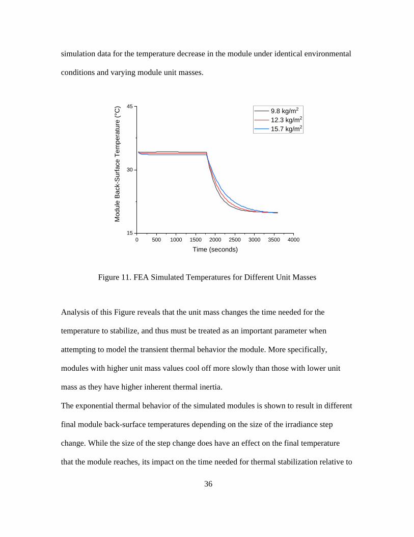
36
simulation data for the temperature decrease in the module under identical environmental
conditions and varying module unit masses.
Figure 11. FEA Simulated Temperatures for Different Unit Masses
Analysis of this Figure reveals that the unit mass changes the time needed for the
temperature to stabilize, and thus must be treated as an important parameter when
attempting to model the transient thermal behavior the module. More specifically,
modules with higher unit mass values cool off more slowly than those with lower unit
mass as they have higher inherent thermal inertia.
The exponential thermal behavior of the simulated modules is shown to result in different
final module back-surface temperatures depending on the size of the irradiance step
change. While the size of the step change does have an effect on the final temperature
that the module reaches, its impact on the time needed for thermal stabilization relative to
0 500 1000 1500 2000 2500 3000 3500 4000
15
30
45
Module
Back-S
urf
ace T
em
pera
ture
(°C
)
Time (seconds)
9.8 kg/m2
12.3 kg/m2
15.7 kg/m2

37
the range of temperatures from the introduction of the irradiance step decrease to the final
simulated time step can be shown to be negligible. The stabilization of the module
temperature to the overall temperature range of the simulated module is evaluated using
the equation shown below:
%𝑆𝑡𝑎𝑏𝑖𝑙𝑖𝑧𝑒ⅆ =|𝑇𝑖−𝑇𝑠𝑡𝑎𝑟𝑡|
|𝑇𝑠𝑡𝑎𝑟𝑡−𝑇𝑓𝑖𝑛𝑎𝑙| (18)
Where 𝑇𝑖 is the temperature at a given time step, 𝑇𝑓𝑖𝑛𝑎𝑙 is the temperature at the final time
step of the simulation, and 𝑇𝑠𝑡𝑎𝑟𝑡 is the initial temperature that the module stabilized to
under the initial irradiance conditions before the step decrease in irradiance was
introduced. The time step at which each FEA simulation’s stabilization values reach 0.1,
or the time needed for the module to reach 90% thermal stabilization, from the
calculation in (17) for different simulation parameters in the summer and spring ambient
temperature conditions are shown in Figure 12. The winter temperatures were neglected
in the analysis as these simulations were found to be less accurate in the steady-state
convergence validation and the ambient temperature was previously determined to have
negligible effects on the shape of the exponential thermal decay.

38
Figure 12. Temperature Stabilization Time for Wind Speed and Unit Mass
These results show that even though the step changes in irradiance cause differences in
the final stabilization temperature, the rate at which the temperature decreases is not
dependent on the size of the irradiance step change. The time required for thermal
stabilization is shown to decrease for increasing wind speed due to the increased cooling
load. The time also increases for higher unit masses due to the higher thermal capacitance
of the module. The small distribution of repeated data points in small clusters in Figure
12 stem from 30 second differences in the required stabilization time for simulations at
the same wind speed and unit mass conditions. These differences could also potentially
be attributed to the different irradiance step change sizes or the different ambient
temperature conditions of the different simulations, but these differences most likely stem

39
from inaccuracies due to the 30 second evaluation intervals within the software.
Regardless of the reason for this small distribution of stabilization times, the temperature
stabilization is far more dependent on wind speed and unit mass than it is on irradiance.
These results are important for the development of the transient temperature prediction
model, as it reveals that the irradiance should not be treated as the primary variable when
accounting for the transient thermal behavior of the module.
The FEA transient simulation method was also used to determine if the trends in module
thermal behavior noted in the analysis of irradiance step decreases could also be applied
to large step increases in irradiance. Performing this analysis required flipping the
irradiance step changes that were used in the decreasing temperature studies in order to
begin the thermal study with a stabilized temperature at low irradiance before introducing
a large step increase in irradiance. The size of the step increases in irradiance are shown
in Figure 13. A sample of these increasing temperature curves is shown in Figures 14
through 16.
Figure 13. Irradiance Step Change Sizes for Increasing Temperature Simulations
0
500
1000
1500
0 900 1800 2700 3600
Inci
den
t Ir
rad
iance
(W
/m²)
Time (seconds)
∆E = 600 W/m²
∆E = 400 W/m²
∆E = 200 W/m²
∆E = 600 W/m²
(Open Circuit)

40
Figure 14. FEA Increasing Temperature Simulations for Spring
0 1000 2000 3000 400015
30
45
60
15
30
45
60
0 1000 2000 3000 4000
15
30
45
60
16°C Ambient Temperature
2 m
/s W
ind
Sp
eed
Time (Seconds)
ΔE = 600 W/m2
ΔE = 400 W/m2
ΔE = 200 W/m2
Mo
du
le B
ack
-Su
rfa
ce T
emp
era
ture
(°C
)
5 m
/s W
ind
Sp
eed
ΔE = 600 W/m2
ΔE = 400 W/m2
ΔE = 200 W/m2
10
m/s
Win
d S
pee
d
ΔE = 600 W/m2
ΔE = 400 W/m2
ΔE = 200 W/m2

41
Figure 15. FEA Increasing Temperature Simulations for Summer
0 1000 2000 3000 400030
40
50
60
30
40
50
60
0 1000 2000 3000 4000
30
40
50
60
32°C Ambient Temperature
2 m
/s W
ind
Sp
eed
Time (Seconds)
ΔE = 600 W/m2
ΔE = 400 W/m2
ΔE = 200 W/m2
Mo
du
le B
ack
-Su
rfa
ce T
emp
era
ture
(°C
)
5 m
/s W
ind
Sp
eed
ΔE = 600 W/m2
ΔE = 400 W/m2
ΔE = 200 W/m2
10
m/s
Win
d S
pee
d
ΔE = 600 W/m2
ΔE = 400 W/m2
ΔE = 200 W/m2

42
Figure 16. FEA Increasing Temperature Simulations for Winter
Analysis of these Figures reveals that the behavior of the module back-surface
temperature is also exponential in nature, with the temperature increasing rapidly
immediately after the step change in irradiance before slowly stabilizing to a final
temperature as time passes. Comparing the temperature performance across different
wind speeds reveals that the wind has the same effect on the module temperature as it
0 1000 2000 3000 4000-5
5
15
25
-5
5
15
25
0 1000 2000 3000 4000
-5
5
15
25
-7°C Ambient Temperature
2 m
/s W
ind
Sp
eed
Time (Seconds)
ΔE = 600 W/m2
ΔE = 400 W/m2
ΔE = 200 W/m2
Mo
du
le B
ack
-Su
rfa
ce T
emp
era
ture
(°C
)
5 m
/s W
ind
Sp
eed
ΔE = 600 W/m2
ΔE = 400 W/m2
ΔE = 200 W/m2
10
m/s
Win
d S
pee
d
ΔE = 600 W/m2
ΔE = 400 W/m2
ΔE = 200 W/m2

43
does in the decreasing temperature studies. Increasing the wind speed incident on the
module front surface flattens the temperature profile of the module, as the increased
cooling load from the wind causes the module temperature to stabilize more quickly.
Evaluating the amount of time needed for the FEA simulated temperature increases to
reach 90% thermal stabilization reveals similar behavior to that found in the decreasing
temperature simulations. The amount of time needed for stabilization is shown as a
function of wind speed and unit mass in Figure 17. Comparing the trends in this Figure
reveal identical behavior to that in Figure 12, with increasing wind speed corresponding
to decreased temperature stabilization time and increased mass per unit area
corresponding to increased stabilization time. The separation in stabilization times for the
same wind speed and unit mass conditions can be attributed to the 60-second data
intervals that were used for these simulations in order to reduce computation time. The
exhibited thermal behavior reveals that the exponential nature of the model applies for
both rapid increases and decreases in temperature, and that the trends in thermal behavior
are shown to be identically dependent on wind speed and unit mass for each direction of
temperature change.

44
Figure 17. Temperature Stabilization Time for Increasing Temperature Simulations
Both the increasing and decreasing FEA module temperature simulation datasets show
that the relative temperature change is dependent on the wind speed and unit mass of the
module rather than the size of the irradiance step change. These trends in module thermal
behavior can be trusted to be reasonably accurate within the inherent accuracy constraints
of the Sandia steady-state module as shown in the steady-state convergence simulations
[4]. This FEA approach ultimately serves as a means of formulating the transient thermal
model that will be discussed in the following sections and is not intended to serve as the
main deliverable of these research efforts. This detailed approach does however offer a
platform for future growth in PV thermal modeling through more detailed finite-element
methods or different computational simulation methods of deriving module transient

45
thermal behavior. Such research efforts may include more detailed computational
simulations of each individual PV module layer’s effect on the thermal mass of modules.
3.5 Moving-Average Model Development
Once the FEA simulations were performed and analyzed, the trends discovered in these
simulations were used to develop a transient thermal model that is based on a few simple
input parameters outside of those easily accessible environmental parameters already
relied on for steady-state modeling. The FEA simulations revealed that the wind speed
and unit mass have a visible and quantifiable effect on the shape of the exponential
temperature decay for the FEA simulated module temperatures. They also showed that
the time needed for the temperature to stabilize to a certain percentage of the overall
thermal gradient is not a function of the irradiance or ambient temperature, which are two
key variables in most steady-state temperature prediction models. This insight into the
dynamic temperature dependence of PV modules can be used to develop a model that can
account for the thermal mass of the module without being over-reliant on the incident
irradiance as an input variable.
The first step in developing the model was to plot the steady-state temperature
predictions made using the Sandia steady-state temperature model [4] to match the FEA
simulated temperatures at the step-change time and the 90% stabilization time. This was
done by first calculating the ambient temperature needed for the steady-state prediction to
match the FEA predicted temperature at the step change point. The irradiance needed for
the steady-state prediction to match the FEA simulated temperature at the 90% thermal
stabilization time was found based on the assumed wind speed and previously calculated
ambient temperatures applied in the Sandia steady-state model to further verify the

46
accuracy of the FEA simulations. The calculated ambient temperature and irradiance
values were determined to be within an acceptable error range to the FEA simulated
curve at these points. This analysis was performed to better understand the difference in
steady-state predicted behavior and expected thermal behavior for modules at narrow
time intervals. An example of this plotting, shown in Figure 18, reveals that the transient
FEA simulations show a reduced temperature ramp rate that is more accurate to how PV
modules would typically be expected to behave in the field for large changes in
irradiance. The steady-state approximations in this Figure are shown to be reasonably
accurate during the beginning and end of the time series when the module is in thermal
equilibrium but show large inaccuracies to the expected module temperature in the
minutes immediately following the step decrease in incident irradiance. The linear
relationship between the irradiance and steady-state temperature predictions leads to step
changes in predicted temperature for step changes in irradiance. As such, these steady-
state modules do not account for the inherent thermal mass of the module. This thermal
mass, treated as a simple function of module weight per unit area in the FEA simulations,
must be accounted for when attempting to accurately predict the module temperature
dynamically.

47
Figure 18. Steady-state Temperature Prediction Inaccuracy as Compared to FEA
Transient Simulation Module Temperatures
With the knowledge that steady-state models such as the Sandia steady-state temperature
model [4] are accurate when the environmental conditions have stabilized to steady-state
operating conditions, there is a benefit to using these accurate steady-state predictions at
past time steps to more accurately predict the temperature for times of intermittent
conditions. This concept resulted in a transient thermal model in which the steady-state
predictions from previous time steps are weighted and averaged in order to predict
module back-surface temperature change with respect to time. The weights attributed to
the steady-state model predictions in this new model are based on the relationship
between module thermal behavior, wind speed, and unit mass that was previously
identified in the FEA. These weights are transient in nature as they take the time of the
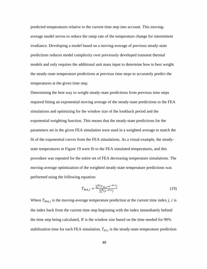
48
predicted temperatures relative to the current time step into account. This moving-
average model serves to reduce the ramp rate of the temperature change for intermittent
irradiance. Developing a model based on a moving-average of previous steady-state
predictions reduces model complexity over previously developed transient thermal
models and only requires the additional unit mass input to determine how to best weight
the steady-state temperature predictions at previous time steps to accurately predict the
temperatures at the given time step.
Determining the best way to weight steady-state predictions from previous time steps
required fitting an exponential moving average of the steady-state predictions to the FEA
simulations and optimizing for the window size of the lookback period and the
exponential weighting function. This means that the steady-state predictions for the
parameters set in the given FEA simulation were used in a weighted average to match the
fit of the exponential curves from the FEA simulations. As a visual example, the steady-
state temperatures in Figure 19 were fit to the FEA simulated temperatures, and this
procedure was repeated for the entire set of FEA decreasing temperature simulations. The
moving-average optimization of the weighted steady-state temperature predictions was
performed using the following equation:
𝑇𝑀𝐴,𝑗 =∑ (𝑇𝑆𝑆,𝑖∗𝑒−𝑃∗𝑖)𝑁
𝑖
∑ (𝑒−𝑃∗𝑖)𝑁𝑖
(19)
Where 𝑇𝑀𝐴,𝑗 is the moving-average temperature prediction at the current time index 𝑗, 𝑖 is
the index back from the current time step beginning with the index immediately behind
the time step being calculated, 𝑁 is the window size based on the time needed for 90%
stabilization time for each FEA simulation, 𝑇𝑆𝑆,𝑖 is the steady-state temperature prediction
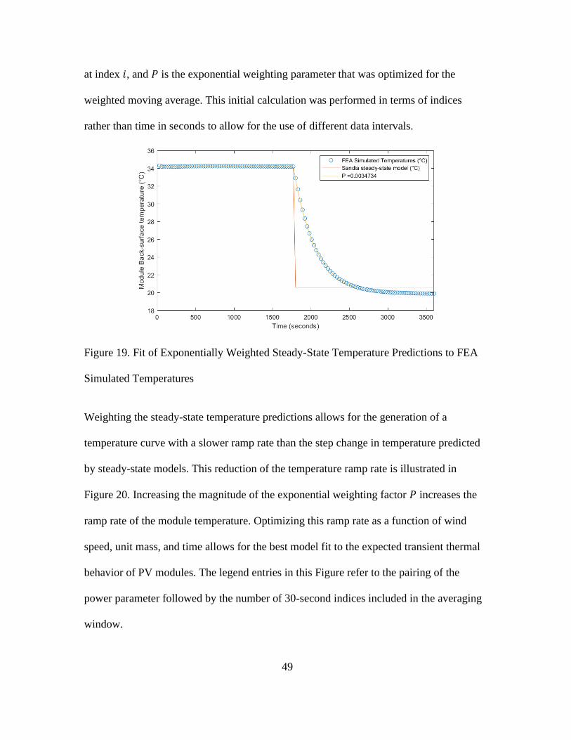
49
at index 𝑖, and 𝑃 is the exponential weighting parameter that was optimized for the
weighted moving average. This initial calculation was performed in terms of indices
rather than time in seconds to allow for the use of different data intervals.
Figure 19. Fit of Exponentially Weighted Steady-State Temperature Predictions to FEA
Simulated Temperatures
Weighting the steady-state temperature predictions allows for the generation of a
temperature curve with a slower ramp rate than the step change in temperature predicted
by steady-state models. This reduction of the temperature ramp rate is illustrated in
Figure 20. Increasing the magnitude of the exponential weighting factor 𝑃 increases the
ramp rate of the module temperature. Optimizing this ramp rate as a function of wind
speed, unit mass, and time allows for the best model fit to the expected transient thermal
behavior of PV modules. The legend entries in this Figure refer to the pairing of the
power parameter followed by the number of 30-second indices included in the averaging
window.
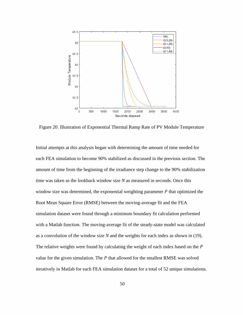
50
Figure 20. Illustration of Exponential Thermal Ramp Rate of PV Module Temperature
Initial attempts at this analysis began with determining the amount of time needed for
each FEA simulation to become 90% stabilized as discussed in the previous section. The
amount of time from the beginning of the irradiance step change to the 90% stabilization
time was taken as the lookback window size N as measured in seconds. Once this
window size was determined, the exponential weighting parameter 𝑃 that optimized the
Root Mean Square Error (RMSE) between the moving-average fit and the FEA
simulation dataset were found through a minimum boundary fit calculation performed
with a Matlab function. The moving-average fit of the steady-state model was calculated
as a convolution of the window size N and the weights for each index as shown in (19).
The relative weights were found by calculating the weight of each index based on the 𝑃
value for the given simulation. The 𝑃 that allowed for the smallest RMSE was solved
iteratively in Matlab for each FEA simulation dataset for a total of 52 unique simulations.

51
2 simulations were found to have inconsistencies in the application of the thermal loads
during the FEA simulations and were thus removed from the original set of 54
simulations of decreasing module temperature.
The resulting weighting function 𝑃 values as they relate to the constant wind speed and
unit mass of the simulated module temperatures are shown in Figure 21. The 𝑃 parameter
was found to increase for increasing wind speed and decrease for increasing unit mass.
The small scatter of the data points in this Figure can again be attributed to the 30 second
data intervals of the FEA simulations and uncertainty in the heat transfer calculations.
Figure 21. Power Parameter as a Function of Wind Speed and Unit Mass
Initial development of the moving-average model was based on the optimization of the
weighting function based on both the window size 𝑁 needed for temperature stabilization
and the weighting function 𝑃 that optimized the fit for the given wind speed and unit

52
mass conditions. Upon further analysis of this initial model optimization, it was
determined that optimizing for two variables in the model equation was overly complex.
As a result, the window size for subsequent analysis was held as a constant of 20 minutes
(1200 seconds) back from the current time step. This assumption was considered
sufficient for the model as the exponential weighting function assigned to the previous
steady-state temperature predictions assigns less weight to those predictions further away
from the current time step, making the predictions furthest away in time negligible in
some cases. 20 minutes was chosen as the constant time based on Figure 12, which shows
that 20 minutes, or 1200 seconds, is more than enough time for each simulation evaluated
to reach temperature stabilization. Increasing this window size beyond 20 minutes did not
show significant accuracy improvements in the optimization. Reducing the window size
risks failure to account for steady-state temperature predictions that are still relevant to
the current module temperature during times of intermittency in the environmental
variables.
With the constant window size determined, the steady-state moving-average fit to the
FEA simulation temperatures could be based solely on the power parameter 𝑃 for the
decreasing temperature studies. The results of the optimization based solely on 𝑃 are
shown in Figure 22 as a 3D plot that relates the wind speed and unit mass to the optimal
power parameter for each simulation. The results show an approximately planar fit
between 𝑃, the wind speed, and the unit mass, with each variable having an
approximately equal importance to the determination of the 𝑃 parameter.
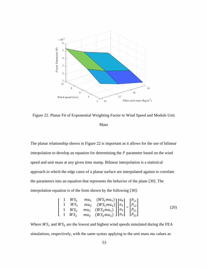
53
Figure 22. Planar Fit of Exponential Weighting Factor to Wind Speed and Module Unit
Mass
The planar relationship shown in Figure 22 is important as it allows for the use of bilinear
interpolation to develop an equation for determining the 𝑃 parameter based on the wind
speed and unit mass at any given time stamp. Bilinear interpolation is a statistical
approach in which the edge cases of a planar surface are interpolated against to correlate
the parameters into an equation that represents the behavior of the plane [30]. The
interpolation equation is of the form shown by the following [30]:
[
1 𝑊𝑆1
1 𝑊𝑆1
𝑚𝑢1 (𝑊𝑆1𝑚𝑢1)𝑚𝑢2 (𝑊𝑆1𝑚𝑢2)
1 𝑊𝑆2
1 𝑊𝑆2
𝑚𝑢1 (𝑊𝑆2𝑚𝑢1) 𝑚𝑢2 (𝑊𝑆2𝑚𝑢2)
] [
𝑎0
𝑎1
𝑎2
𝑎3
] = [
𝑃11
𝑃12
𝑃21
𝑃22
] (20)
Where 𝑊𝑆1 and 𝑊𝑆2 are the lowest and highest wind speeds simulated during the FEA
simulations, respectively, with the same syntax applying to the unit mass mu values as

54
well. The 𝑃ij values represent the 𝑃 value calculated to fit the model to the FEA
simulation performed with wind speed i and unit mass j. The resulting coefficients a0-a3
can be used to calculate the weight parameter P at any wind speed and unit mass through
the following [30]:
P = a0 + a1*WS + a2*mu + a3*WS*mu (21)
Performing bilinear interpolation for the edge cases of the planar fit shown in Figure 22
led to the following bilinear interpolation coefficients shown in Table 3. Reapplying the
coefficients to the test conditions of the entire decreasing temperature FEA dataset led to
P prediction accuracy of 1e-4 for those simulations contained within the edge cases used
for the analysis. With the model weighting factor now able to be determined at any given
time step, the final model was implemented in a manner that would be easily accessible
to industry and relevant software packages.
Table 3. Bilinear Interpolation Coefficients for Exponential Weighting Factor
3.6 Model Implementation
The optimization and resulting bilinear interpolation of the weighting parameter for the
weighted moving-average of steady-state temperatures allows for the calculation of the
dynamic module back-surface temperatures for any planar module. The final model
Coefficient Value
a0 0.0046
a1 0.00046
a2 -0.00023
a3 -1.6E-05

55
equation that was formed as a result of the optimized fit between the weighted moving-
average of steady-state temperature predictions and the FEA simulated module back-
surface temperatures is shown below:
𝑇𝑀𝐴,𝑖 =∑ (𝑇𝑆𝑆,𝑖∗𝑒−𝑃∗𝑡𝑖)
𝑡𝑖≤1200
𝑖=2
∑ (𝑒−𝑃∗𝑡𝑖)𝑡𝑖≤1200
𝑖=2
(22)
Where 𝑖 is the index of the time step relative to index 𝑖 = 1 of the current time step being
evaluated, 𝑇𝑀𝐴,𝑖 is the moving-average model module back-surface temperature
prediction (°C) at index 𝑖, 𝑡𝑖 is the time in seconds that the indexed time step is from the
current time step, and 𝑃 is the weighting factor calculated for the wind speed and unit
mass at the current index. This final model equation contains an exponentially weighted
average that is of the same form as the optimization model used to define the exponential
weighting factor 𝑃.
The final equation is based on the time in seconds rather than an index location relative to
the given time step in order to allow for the use of the model for data on any time interval
and to account for missing time steps in a dataset. In this equation, the summation terms
included in the averaging window start at index 𝑖 = 2, which is the index immediately
behind the point in time being considered. This notation helps to more clearly
demonstrate the fact that the model is based on a moving-average of steady-state
temperatures behind the time in questions and does not include the steady-state
temperature prediction for the given instant in the calculation. The steady-state
predictions used in this model are assumed to describe the temperature conditions of the
PV module in the time interval following the index in question rather than the preceding
time interval. For the scenario where the steady-state calculations described the thermal

56
conditions forward in time, the steady-state temperature prediction at the index being
considered would describe temperature conditions for a time that has not yet occurred,
and thus this steady-state prediction cannot be used in the calculation. The moving-
average model equation is the main deliverable of the thesis work, as it the ultimate
model equation that was developed in order to address the gap in transient thermal
modeling of PV modules.
The use of unit mass (mass per unit area) as a primary input to the model allows for this
model to be applied to thermal analysis of any planar PV module regardless of the
materials used in module construction and the type of solar cells being used. The unit
mass serves as a substitute for the thermal capacitance of the numerous layers contained
within any planar PV modules by linking the transient thermal behavior to total weight
per unit rather than specific material thermal properties that can be difficult to define for
each layer. Applying the model to a given module first requires the calculation of the
mass per unit area by dividing the overall mass of the module in kilograms by the surface
area in square meters as listed in the module’s spec sheet.
Applying the moving-average model next requires the calculation of steady-state
temperature predictions for every timestamp in the dataset being analyzed. These steady-
state predictions can be performed using any validated steady-state temperature model.
Empirically optimizing these models based on previous temperature data for the module
at the desired array site can offer improved modeling accuracy for both the steady-state
and moving-average models. If such optimization cannot be performed, the moving-
average model should still offer improved modeling accuracy over steady-state models
using default or generalized coefficients.

57
The other primary input to the moving-average model is the wind speed at the array site.
This wind speed should ideally be measured at approximately the same height as the
module to have a true measure of the wind incident on the modules. If the wind is
measured at a height significantly different from that of the module height, the wind
speed measurements can be adjusted to the desired height. The following conversion
must be made to convert wind speeds at various heights to the correct measurement
height [31]:
𝑣(𝑧) = 𝑣(𝑧𝑟)ln(
𝑧
𝑧0)
ln(𝑧𝑟𝑧0
) (23)
Where 𝑣(𝑧) is the wind speed vector at the desired measurement height 𝑧 (meters) in
m/s, 𝑣(𝑧𝑟) is the wind speed vector at the reference height 𝑧𝑟 (meters), and 𝑧0 is the
roughness length of the PV array site in meters [31]. The roughness length is the
theoretical height in meters at which the wind speed could be expected to be zero [31].
The wind roughness length in this analysis was assumed to be 0.25 meters, which is
analogous with an environment with scattered large buildings or obtrusions [31].
An example of the moving-average model calculations is shown in Table 4. This example
data is based on measurements taken on a 2-minute interval. The module being analyzed
was a rectangular module with a glass front and polymer backsheet that was found to
have a total weight of 18.2 kg and dimensions of 1.650 meters by 0.992 meters. These
values result in a unit mass of 11. 1 kg/m2.

58
Table 4. Moving-Average Model Example Calculation
The rows of the table indicate the index of each data point relative to index 1, which is
the time index for which the module temperature is being calculated. The data between
t = 480s and t = 840s is intentionally excluded in this example to show that the model still
works for nonuniformly sampled data or data with missing time stamps. The numerator
of the moving-average model equation in (22) is found from the steady-state temperature
predictions in Table 4 for each index outside of the first index, the time values for each
index outside of the first index, and the 𝑃 value calculated for the unit mass of the
module and the wind speed at the first index. The denominator in (22) is calculated
similarly except the steady-state temperatures are not included. These calculations, shown
in the equation below, led to the moving-average temperature prediction in °C for the
first index in Table 4:
𝑇𝑀𝐴 =[22.5𝑒−𝑃∗120]+[26.2𝑒−𝑃∗240]+[28.7𝑒−𝑃∗480]+⋯[19.0𝑒−𝑃∗1200]
[𝑒−𝑃∗120]+[𝑒−𝑃∗240]+[𝑒−𝑃∗480]+⋯[𝑒−𝑃∗1200] (24)
This procedure is used for each timestep in a given dataset to calculate the moving-
average temperature predictions of any given module over a time period.
One useful implementation of this model is to apply it to an annual dataset from either
measured or historically averaged environmental data in order to model the expected PV
TABLE III MOVING-AVERAGE MODEL EXAMPLE CALCULATION
Time
index, i
SECONDS
BEFORE
t=0, ti
Steady State
Temp. TSS,i
(°C)
2-meter
Wind
Speed
(m/s)
Pi TMA, i
(°C)
Pi
1 0 32.5 5.0 0.0032 22.5 0.0035
2 120 22.5 N/A N/A N/A N/A
3 240 26.2 N/A N/A N/A N/A
4 480 28.7 N/A N/A N/A N/A
5 840 19.0 N/A N/A N/A N/A
6 960 18.2 N/A N/A N/A N/A
7 1080 18.3 N/A N/A N/A N/A
8 1200 19.0 N/A N/A N/A

59
array output for a given site. Applying the model in this way first requires calculating the
input parameters of steady-state temperature, wind speed, and unit mass as described in
the example shown in Table 4. The model runs by first calculating the 𝑃 parameters for
each time stamp in the dataset by using the bilinear interpolation coefficients in Table 3,
converted wind speed values, and the unit mass. The first-time stamp in the dataset is
automatically set to the steady-state predicted temperature value as there are no previous
time stamps to perform a moving-average across. Because of this, the dataset being
evaluated should start during a time of stable module temperature. For an annual dataset,
the dataset typically starts from midnight of January 1st, which would be characterized by
a prolonged period of zero incident irradiance and stable module temperatures that can be
accurately predicted through steady-state models. For the remainder of the dataset, the
model function is designed to loop through each index in the dataset, find all steady-state
temperature predictions within the 20-minute (1200 seconds) window preceding the time
stamp at said index, and perform a weighted moving-average on all predictions that are
found using the 𝑃 value calculated for the wind speed of that index.
The indexing for the moving-average model is done by using front and back index
markers on the dataset. Each iteration of the loop places the front index at the time stamp
immediately prior to that of the current index and places the rear index at the furthest
possible index that has a time stamp within 20 minutes of the current index’s timestamp.
This indexing system eliminates the need for searching through the entire dataset for data
to include in the moving-average at each index based on the time stamp data by
essentially creating a subset of values within. The indices generate a subset of the dataset
at each loop containing all possible previous time stamps for consideration, then allows

60
the steady-state predictions within the index to be averaged. This system saves processing
time when modeling and allows for predictions of module back-surface temperature for
annual datasets to be generated within seconds.
The original model implementation was performed in Matlab as a function that could be
called for input parameters including timestamps, steady-state temperature predictions,
wind speed values, unit mass conditions, and optional alternatives to the previously
determined bilinear interpolation coefficients. As this is a transient temperature model,
the time stamps of the data being evaluated must be formatted such that they can be used
in the calculations. The Matlab formatting of the time stamps matched that of the
software package PVLIB, a package of PV performance modeling equations [32]. The
time stamps that must be input into the moving-average model function must be
formatted as time structs, which are Matlab variables consisting of classes containing the
year, month, day, hour, minute, and second data for each time step in the dataset along
with a UTC offset to set the time zone of the data.
The moving-average temperature model was also written to be used in Python as part of
the PVLIB distribution on that platform. The Python version of the model relies on the
Pandas package of statistical tools. Pandas allows for the model inputs to be converted
into a Pandas DataFrame, a table that is indexable by time stamp or by index location
[33]. The remainder of the code functions in the same way as the Matlab function, with
the mathematical operations required in the Python version being handled by the NumPy
package of mathematical functions [34].

61
CHAPTER 4
RESULTS AND DISCUSSIONS
The transient moving-average thermal model must be validated against measured module
temperature data to prove that the model is accurate enough to be implemented into PV
performance modeling practices in the future. This validation quantifies the accuracy of
the transient model temperature predictions against module back-surface temperatures
measured at PV sites with different climate conditions and module types. The validation
also shows how the use of the moving-average filter in the model provides a much
smoother and accurate temperature prediction curve for narrow data intervals than the
steady-state models commonly used in performance modeling. Improvements in the
thermal modeling accuracy are also linked back to performance, with calculations
showing what effect the accuracy improvements have on the expected accuracy of overall
PV performance calculations. The following subsections will discuss the various
statistical and graphical analyses performed for the transient thermal model along with
conclusions that can be drawn based on the results of said analyses.
4.1 Data Handling
A large portion of the moving-average model validation is based on PV and
environmental data collected and maintained at Sandia National Laboratories’
Photovoltaic System Evaluation Laboratory (PSEL) in Albuquerque, NM. Data from four
PV sites with unique climate conditions were evaluated in order to inspect the
performance of the model for differing degrees of solar intermittency, ambient
temperature conditions, and wind conditions. The four sites were as follows:
Albuquerque, NM, Orlando, FL, Las Vegas, NV, and Williston VT. The PV arrays that

62
the data from these sites was taken from were of the same size and module construction
type in order to ensure proper comparison of the experimental analyses. The modules
chosen for each of these sites each consisted of a glass front surface and polymer
backsheet. Each module was set at a tilt angle equal to the respective site’s latitude and
an azimuth angle of 180° from due North that caused the modules to be pointed due
South. The data for each site was measured in 1-minute intervals using standard
datalogger equipment and technologies. The datasets covered a full calendar year of data,
with some sites having periods of maintenance or downtime in which the data was
missing and not considered in the analysis. Further data filtering methods aimed at
ensuring a true representation of the benefits of the moving-average model are described
below.
4.2 Data Filtering
The moving-average nature of the model requires the use of an existing steady-state
model in order to eventually arrive at the desired transient thermal predictions for the
given time steps. In this analysis, the previously mentioned Sandia steady-state
temperature model is used for the moving-average model calculations [4]. The steady-
state model coefficients were optimized for each site in order to form an optimal
comparison of the steady-state and moving-average model based on steady-state
modeling that is a true fit to the expected module thermal behavior of the given climate.
Using the default steady-state coefficients provided in [4] for the moving-average model
calculations would still show improvements in the modeling accuracy. The optimization
was based on a minimum boundary fit for the steady-state model coefficients that
minimized the Root Mean Square Error (RMSE) for the difference between the measured
63
and steady-state modeled temperature data. This optimization was performed for annual
temperature datasets for each location that were filtered to only include daytime time
stamps in which there were clear sky conditions with low intermittency in incident
irradiance. The clear sky filtering was performed using a function within PVLIB that uses
solar position algorithms and changes in the measured global horizontal irradiance (GHI)
over time to find the time stamps within a dataset that can be considered to have clear sky
conditions [32], [35]. The function compares measured GHI data over a sliding time
window to values predicted by the Ineichen clear sky model, which predicts the GHI of a
given site using the following system of equations [35], [36]:
𝐺𝐻𝐼 = 𝑐𝑔1 ∗ 𝐼0 ∗ cos(𝑧) ∗ exp (−𝑐𝑔2 ∗ 𝐴𝑀 ∗ (𝑓ℎ1 + 𝑓ℎ2(𝑇𝐿 − 1))) ∗ exp (0.01 ∗ 𝐴𝑀1.8) (25)
𝑓ℎ1 = exp (−ℎ
8000) (26)
𝑓ℎ2 = exp (−ℎ
1250) (27)
𝑐𝑔1 = 5.09 ∗ 10−5 ∗ ℎ + 0.868 (28)
𝑐𝑔2 = 3.92 ∗ 10−5 ∗ ℎ + 0.0387 (29)
Where 𝐼0 is the extraterrestrial irradiance constant, 𝑧 is the solar zenith angle in radians,
𝐴𝑀 is the air mass, 𝑇𝐿 is the Linke turbidity factor, and ℎ is the elevation of the site in
meters. The coefficients in (25)-(28) were determined empirically based on elevation
[35], [36]. The turbidity factor 𝑇𝐿 is a measure of the scattering and absorption of light
by water particles and aerosols that Ineichen calculates independently of the air mass
[36], [37].
Optimizing for only clear sky conditions ensures that the steady-state model temperature
is optimized for module temperatures that are stable in nature and not affected by

64
intermittent irradiance, as these are the conditions under which the model has been
proven accurate [4], [22]. The final optimized coefficients for each dataset were then
used for the steady-state modeling across the full year of data, which was subjected to
numerous data filters but was not limited to only clear sky conditions.
For a true understanding of the benefits of the moving-average model, each dataset was
filtered to include only those time stamps with logical values for the variables of
importance in the calculation. These variables included the POA irradiance, ambient
temperature, wind speed, GHI, and measured module temperature for comparison
purposes. The dataset was first filtered to eliminate time steps where any of these
variables were missing due to datalogger communication errors or nonfunctioning data
sensors. Next, each of the relevant values were filtered to eliminate any values that were
outside of the expected range of expected behavior. For example, module temperatures
would typically be expected to reach as high as 30°C above the ambient temperature
based on steady-state predictions, so any reported temperatures exceeding that value
would indicate an issue with the sensor or data collection methods. In the case of module
temperature, this could be the result of the measurement apparatus losing contact with the
module or being in open circuit condition due to a disconnected lead. Measurements of
the wind speed magnitude were filtered to exclude any negative values that are physically
impossible. The irradiance values were filtered to exclude values less than 0 W/m2 or
greater than 1500 W/m2. The ambient temperature measurements were filtered to remove
impossible or unrealistic values based on the expected ranges of ambient temperatures.
After filtering for both missing and impossible data, the times at which the measured
environmental data is relevant to PV performance were also considered. As PV energy

65
production at the module level can only occur when there is irradiance hitting the PV
cells, times after the sun has set each day and before it has risen in the morning are not
relevant when considering the accuracy of PV temperature modeling. In order to generate
statistics showcasing the accuracy of the model solely for times of production, the data
was filtered to eliminate the irrelevant nighttime data from the dataset. Rather than
filtering based on arbitrary constant start and stop times each day that would have to be
changed for the different time zones in each climate, the data was filtered based on solar
position calculations of the angle of incidence (AOI) between the sun and the module
surface plane. The AOI is the angle at which light hits the module front surface. This
value changes for modules at a fixed tilt angle as the sun’s position relative to the module
changes throughout the day [10]. The AOI for each site was calculated at each time step
using equations from PVLIB that were based on the following equations for planar
modules [10], [32]:
𝐴𝑂𝐼 = 𝑐𝑜𝑠−1[cos(𝜃𝑍) cos(𝜃𝑇) + sin (𝜃𝑍) sin (𝜃𝑇)cos (𝜃𝐴 − 𝜃𝐴,𝑎𝑟𝑟𝑎𝑦)] (30)
Where 𝐴𝑂𝐼 is the angle of incidence, 𝜃𝑍 is the solar zenith angle, 𝜃𝑇 is the tilt angle of
the PV array, 𝜃𝐴 is the solar azimuth angle, and 𝜃𝐴,𝑎𝑟𝑟𝑎𝑦 is the azimuth angle of the array.
To exclude times when the sun is rising and setting and there is not yet a huge amount of
irradiance falling on the module, AOI values greater than 75° were excluded from the
analysis. Additionally, the elevation angle of the sun, a parameter signifying the height of
the sun relative to the horizontal [10], was considered for the analysis for the
Albuquerque, NM dataset. This was done by only including data with elevation angles
greater than 10° to eliminate data for times in which the sun has not yet crested the
mountains near the PV array site stationed at Sandia National Laboratories from which

66
the data was collected. This additional filter was not applied to the other datasets as there
was no evidence of large obstructions near the PV installations that required additional
considerations into the solar positioning.
Once all the data filters were applied, the steady-state temperature approximations for the
remaining dataset were calculated with the optimized coefficients determined in the clear
sky analysis. The wind speed measurements were corrected to a height of 2 meters and
the module unit mass was calculated from the module spec sheets to be approximately 11
kg/m2 [38]. These wind and unit mass values, along with the time struct containing the
time step data and the steady-state temperature predictions, were entered into the moving-
average model function to generate an array of transient module back-surface
temperature predictions. This model output array could then be evaluated based on its
performance relative to measured module temperatures and to the model residuals
expected from steady-state temperature models.
4.3 Cumulative Distribution Function Analysis
Empirical Cumulative Distribution Function (CDF) analysis is used to show how likely a
variable is to be under a given threshold value [39]. In the case of the moving-average
model, the CDF analysis can be used to see how likely the absolute residuals between the
transient thermal model and module back-surface temperature measurements are to be
within 2°C, 5°C, or any arbitrary temperature residual value that would be representative
of the accuracy desired for the given PV performance modeling efforts. An issue with
steady-state temperature models, particularly at frequent data intervals such as 1-minute,
is that they vary widely with changing irradiance, which leads to more instances of large
model residuals to measured data. Smoothing out the temperature prediction curve

67
through a moving-average of the predictions from previous time steps can eliminate the
spiking exhibited in these steady-state models at narrow time scales.
The CDF analysis was used to show how the moving-average model could improve upon
the variability of the steady-state model for data ranging in frequency from 1-minute to
10-minute data. These different data intervals were generated from Albuquerque, NM
annual dataset of 1-minute data. The data was resampled into intervals of 2 minutes, 3
minutes, 4 minutes, 5 minutes, 7 minutes, and 10 minutes using Matlab’s timetable
functionality to resample the relevant variables through averaging of data points within
the new data sampling interval. The transient thermal model was run for each data
interval, and the results were compared against the similarly resampled module
temperature data measurements by taking the absolute value of the difference between
measured and modeled temperatures for each test case. CDF analysis was performed on
each set of absolute residuals, with the results plotted in Figure 23.

68
Figure 23. Empirical CDF Analysis of Moving-Average Model Fit to Albuquerque Data
Analysis of this Figure reveals that approximately 95% of the moving-average model
residuals for 1-minute data can be expected to be under 5°C, with the subsequent data
intervals having a gradual decrease in accuracy. The 10-minute dataset is found to have
approximately the same residual probability curve as a purely steady-state temperature
model, which aligns with the expectations of the 20-minute averaging window of the
model. The 20 minute-window leads to a maximum of 2 data points being included in the
averaging window, which results in a model that is very similar to that of the steady-state
model. Extending the averaging window poses the risk of basing the temperature
prediction at the current time step on temperatures at time steps that are not relevant to
the current time based on the transient thermal behavior observed in the FEA analysis.
This CDF plot shows that the moving-average model offers significantly reduced

69
modeling variability for more narrow data intervals ranging from less than a minute to 10
minutes.
4.4 Moving-Average Model Fit to Measured Data
The four different PV array sites were evaluated based on how the temperature
predictions calculated using the moving-average model compared to measured
temperature data from each site. The statistical analysis of this fit between modeled and
measured temperatures was based on the comparison of numerous fit statistics
quantifying the accuracy of both the moving-average model and steady-state temperature
model. These fit statistics included Root Mean Square Error (RMSE), which is a measure
of the average deviation of the predicted temperatures to the measured temperatures
across the annual dataset. The RMSE values in °C found in this analysis were based on
the following equation [40]:
𝑅𝑀𝑆𝐸 = √∑(𝑇𝑚𝑒𝑎𝑠𝑢𝑟𝑒𝑑− 𝑇𝑚𝑜𝑑𝑒𝑙)2
𝑛 (31)
Where 𝑇𝑚𝑒𝑎𝑠𝑢𝑟𝑒𝑑 is the measured module back-surface temperatures for the site in °C,
𝑇𝑚𝑜𝑑𝑒𝑙 is either the steady-state or moving-average modeled temperatures in °C, and 𝑛 is
the number of samples in the dataset for the given site [40]. The statistical analysis also
includes Mean Bias Error (MBE), an overall average of the residuals across the full
dataset that reveals underprediction or overprediction bias for the model through the sign
of the value. The MBE values for both the steady-state and moving-average models were
found using the following equation [40]:
𝑀𝐵𝐸 = ∑(𝑇𝑚𝑒𝑎𝑠𝑢𝑟𝑒𝑑− 𝑇𝑚𝑜𝑑𝑒𝑙)
𝑛 (32)

70
Negative MBE values indicate that the temperature model tends to predict module
temperatures higher than the actual measured values. Alternatively, large positive values
would indicate that the temperature model is predicting temperatures lower than that of
the measured temperatures [40]. A statistic that is similar to MBE is Mean Absolute Error
(MAE), which shows the absolute average residuals to give a true value to the inherent
accuracy of the models [40]:
𝑀𝐴𝐸 = ∑|(𝑇𝑚𝑒𝑎𝑠𝑢𝑟𝑒𝑑− 𝑇𝑚𝑜𝑑𝑒𝑙)|
𝑛 (33)
The MAE differs from the MBE in that it shows the absolute difference in the measured
and modeled temperatures eliminating any bias from the direction of the temperature
residuals. The difference between the RMSE and MAE values represent the amount of
variance in the residuals, with higher amounts of large error in temperature predictions
causing a greater difference between the statistics due to the square nature of the RMSE
calculation [40]. The R2 fit of the data also reveals how good of a fit each temperature
model is to the known temperature models. The R2 calculations for the model validation
were performed using the following equation [40]:
𝑅2 = 1 − ∑(𝑇𝑚𝑒𝑎𝑠𝑢𝑟𝑒𝑑− 𝑇𝑚𝑜𝑑𝑒𝑙)2
∑(𝑇𝑚𝑒𝑎𝑠𝑢𝑟𝑒𝑑− ∑ 𝑇𝑚𝑒𝑎𝑠𝑢𝑟𝑒𝑑
𝑛)2
(34)
The calculated values of these different fit statistics for each of the four PV sites are
shown in Table 5.

71
Table 5. Fit statistics for Moving-Average Model and Steady-State Models for Different
Climates
Analysis of this table shows that the implementation of the moving-average model
improves the statistical fit of the predicted temperatures to the measured data for each of
the four unique climate conditions. The improvements show that the moving-average
model improvements are greatest for the temperate climate of Orlando, which is
characterized by frequent times of solar intermittency that would lead to high variance
and inaccuracy when using purely steady-state models to predict module temperatures.
The benefits of the moving-average model appear to be the smallest for areas with
weather conditions like Las Vegas, which is characterized by large amounts of irradiance
and fewer times of intermittency caused by cloud cover or storms. In each climate, the
Albuquerque
Optimized SS Moving-Average
RMSE (°C) 3.79 2.69
MAE (°C) 2.86 2.14
MBE (°C) -0.442 -0.341
R-Squared 0.936 0.967
Orlando
Optimized SS Moving-Average
RMSE (°C) 4.41 2.03
MAE (°C) 3.02 1.57
MBE (°C) 0.326 0.318
R-Squared 0.880 .975
Vermont
Optimized SS Moving-Average
RMSE (°C) 3.92 2.90
MAE (°C) 2.86 2.20
MBE (°C) -0.86 -0.83
R-Squared 0.9596 0.977
Las Vegas
Optimized SS Moving-Average
RMSE (°C) 2.86 2.22
MAE (°C) 2.20 1.80
MBE (°C) -0.380 -0.296
R-Squared 0.968 0.981

72
implementation of the moving-average model decreases the difference between RMSE
and MAE to a value less than 1°C, which shows reduced prediction variability for the
transient model as compared to the steady-state model variance.
Studying the trends in the MBE reveals that there is a general trend for the model to
predict module back-surface temperatures greater than the measured temperatures for
most of the climates when evaluating over the full year. The MBE for Orlando shows a
slightly positive value that is very close to zero. Overall, the fact that the MBE for each
location is within 1°C of zero and the MAE is within 2°C shows that the moving-average
model accurately predicts module temperature across a wide range of climate conditions.
Seasonal examples of the effect the moving-average model has on days that are
characterized by solar intermittency are shown in Figures 24 and 25. Figure 24 shows a
summer day in Albuquerque where the module temperature varies throughout the day as
a function of prolonged periods of decreased irradiance. Looking at the steady-state fit to
the measured data for these days, the predicted temperatures spike from low to high
based on minute-to-minute changes in the plane-of-array irradiance measurements. Using
the moving-average model as a smoothing filter over these steady-state predictions serves
to reduce the variability of these predictions while also much more accurately matching
the measured temperature curve. Visual inspection of this plot shows that the moving-
average modeled temperatures closely follows the shape of the measured module
temperatures. While there are times during this summer day in which there is a noticeable
offset between the moving-average model predictions and the measured temperatures, the
shape of the predicted module temperatures is still nearly the same as that of the
measured temperature.

73
Figure 24. Summer Example of Moving-Average Model Fit to Measured Data
(Albuquerque)
Figure 25 shows the same model comparison for a winter day. Just as in Figure 24, the
moving-average model follows the shape of the measured module back-surface
temperatures curve more closely than the steady-state model. While the shape of the
moving-average curve closely follows the measured temperatures, there is an offset that
shows moving-average model predicts temperatures higher than the measured
temperatures early in the morning. This offset can again be attributed to inherent
inaccuracies in the steady-state thermal model.

74
Figure 25. Winter Example of Moving-Average Model Fit to Measured Data
(Albuquerque)
The benefits of the moving-average model can also be shown for steady-state calculations
performed with default coefficients. The degree to which the steady-state model is
optimized to a given array site only effects the starting point of the model error relative to
the measured temperatures and should not change the degree to which the moving-
average filter improves the modeling accuracy. This is shown in Table 6, which shows
the moving-average and steady-state model fits for the default Sandia steady-state
coefficients of a = -3.56 and b = -.075.

75
Table 6. Fit Statistics for Moving-Average and Default Steady-State Model for Different
Climates
These results show decreased improvement in the modeling accuracy provided by the
moving average model, as the steady-state model is much less accurate during times of
stable environmental conditions. This means that the moving-average model is often
basing its temperature predictions on a weighted average of inaccurate temperature
measurements. The positive MBE values for each dataset show that the default steady-
state model underpredicts module temperature consistently, which may be due to the
increased b coefficient value which increases the effect of the wind speed on the
temperature calculation.
Albuquerque
Default SS Moving-Average
RMSE (°C) 5.26 4.79
MAE (°C) 4.09 3.81
MBE (°C) 2.90 3.00
R-Squared 0.876 0.897
Orlando
Default SS Moving-Average
RMSE (°C) 6.42 5.65
MAE (°C) 5.08 4.79
MBE (°C) 4.61 4.61
R-Squared 0.746 0.803
Vermont
Default SS Moving-Average
RMSE (°C) 5.36 4.90
MAE (°C) 3.97 3.71
MBE (°C) 2.29 2.32
R-Squared 0.922 0.936
Las Vegas
Default SS Moving-Average
RMSE (°C) 4.49 4.19
MAE (°C) 3.56 3.42
MBE (°C) 2.62 2.71
R-Squared 0.921 0.932
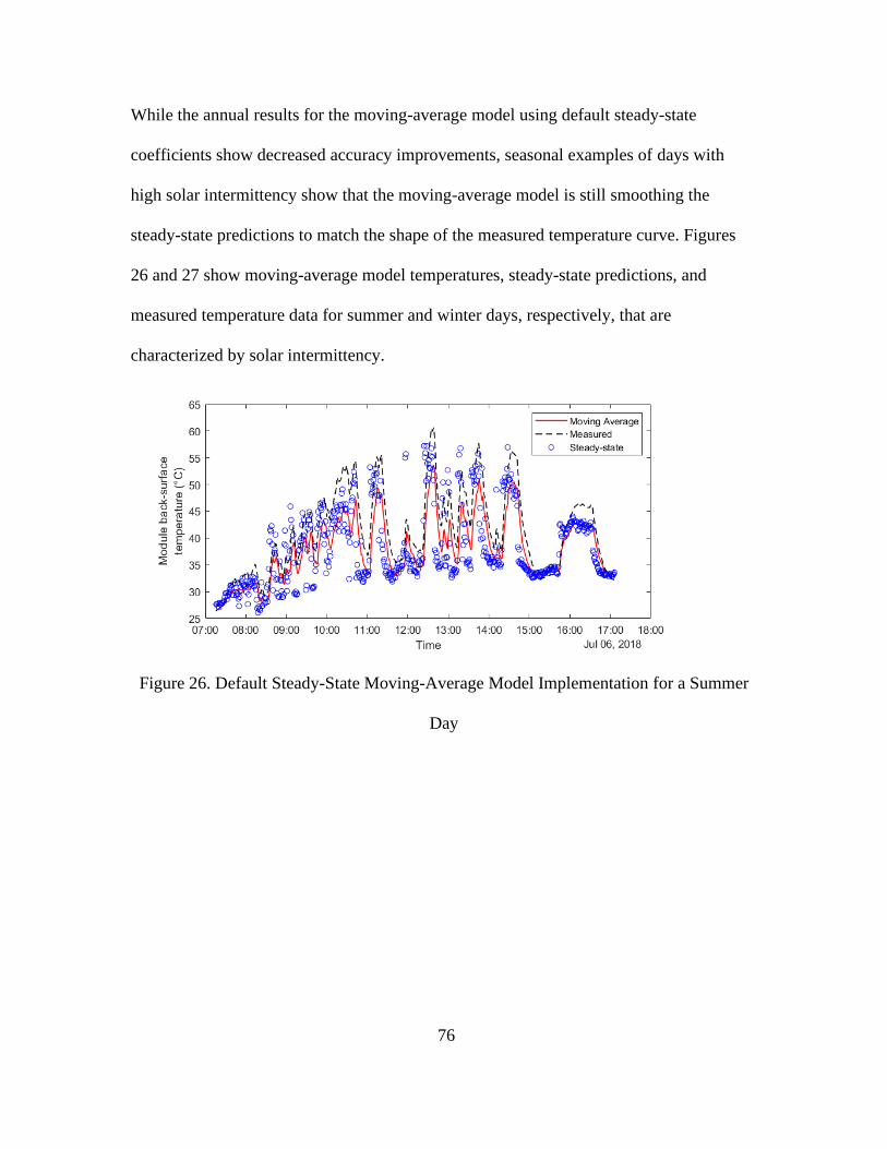
76
While the annual results for the moving-average model using default steady-state
coefficients show decreased accuracy improvements, seasonal examples of days with
high solar intermittency show that the moving-average model is still smoothing the
steady-state predictions to match the shape of the measured temperature curve. Figures
26 and 27 show moving-average model temperatures, steady-state predictions, and
measured temperature data for summer and winter days, respectively, that are
characterized by solar intermittency.
Figure 26. Default Steady-State Moving-Average Model Implementation for a Summer
Day
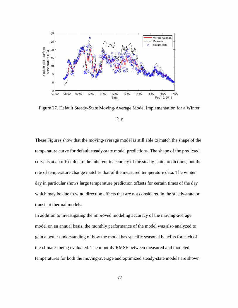
77
Figure 27. Default Steady-State Moving-Average Model Implementation for a Winter
Day
These Figures show that the moving-average model is still able to match the shape of the
temperature curve for default steady-state model predictions. The shape of the predicted
curve is at an offset due to the inherent inaccuracy of the steady-state predictions, but the
rate of temperature change matches that of the measured temperature data. The winter
day in particular shows large temperature prediction offsets for certain times of the day
which may be due to wind direction effects that are not considered in the steady-state or
transient thermal models.
In addition to investigating the improved modeling accuracy of the moving-average
model on an annual basis, the monthly performance of the model was also analyzed to
gain a better understanding of how the model has specific seasonal benefits for each of
the climates being evaluated. The monthly RMSE between measured and modeled
temperatures for both the moving-average and optimized steady-state models are shown

78
in Figures 28 - 31, with each Figure showing the results for the different PV array sites as
discussed in for the optimized steady-state and moving-average model results in Table 5.
Figure 28. Monthly RMSE for Moving-Average and Steady-State Models (Albuquerque)
Analysis of Figure 28 for the Albuquerque array shows that introducing the moving-
average model has increased benefits on modeling accuracy for the spring and summer
months. The absence of August model performance stems from the lack of data for that
month due to system maintenance. The moving-average model is shown to have the
smallest effect in the colder months such as November and January that are characterized
by less available irradiance.

79
Figure 29. Monthly RMSE for Moving-Average and Steady-State Models (Orlando)
Analysis of the data for the Orlando, Florida site shown in Figure 29 shows large RMSE
improvements in the range of 3°C for summer conditions. There are also significant
modeling accuracy improvements across the year for this type of climate. The frequent
solar intermittency present in the temperature conditions of Orlando provides a clear
example of the need to account for transient thermal behavior in PV modules over narrow
data intervals.
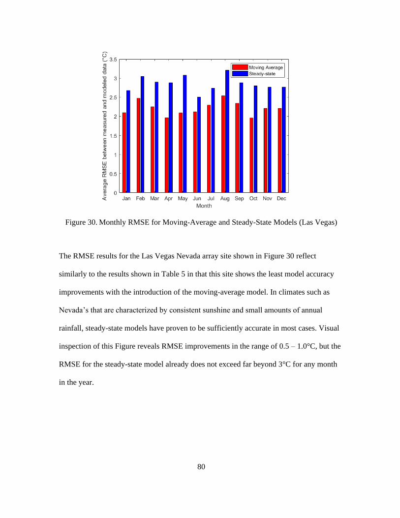
80
Figure 30. Monthly RMSE for Moving-Average and Steady-State Models (Las Vegas)
The RMSE results for the Las Vegas Nevada array site shown in Figure 30 reflect
similarly to the results shown in Table 5 in that this site shows the least model accuracy
improvements with the introduction of the moving-average model. In climates such as
Nevada’s that are characterized by consistent sunshine and small amounts of annual
rainfall, steady-state models have proven to be sufficiently accurate in most cases. Visual
inspection of this Figure reveals RMSE improvements in the range of 0.5 – 1.0°C, but the
RMSE for the steady-state model already does not exceed far beyond 3°C for any month
in the year.
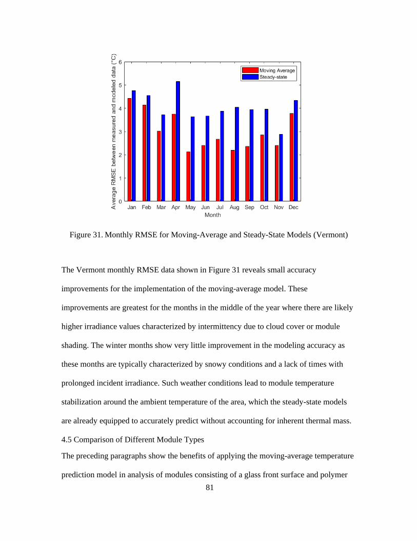
81
Figure 31. Monthly RMSE for Moving-Average and Steady-State Models (Vermont)
The Vermont monthly RMSE data shown in Figure 31 reveals small accuracy
improvements for the implementation of the moving-average model. These
improvements are greatest for the months in the middle of the year where there are likely
higher irradiance values characterized by intermittency due to cloud cover or module
shading. The winter months show very little improvement in the modeling accuracy as
these months are typically characterized by snowy conditions and a lack of times with
prolonged incident irradiance. Such weather conditions lead to module temperature
stabilization around the ambient temperature of the area, which the steady-state models
are already equipped to accurately predict without accounting for inherent thermal mass.
4.5 Comparison of Different Module Types
The preceding paragraphs show the benefits of applying the moving-average temperature
prediction model in analysis of modules consisting of a glass front surface and polymer

82
backsheet rear surface. As the FEA simulations that the model was developed from
assumed that glass makes up the majority of the weight of PV modules, analysis of
modules with different material compositions and weights must be performed to show the
accuracy of the model for different module weights. Many different types of PV modules
are currently in production throughout the world based on different back-surface
compositions and PV cell types. Many PV cell technologies are encased within two
sheets of glass in a module construction that does not include a polymer backsheet.
Bifacial modules that allow for increased cell efficiency through the absorption of
ground-reflected light hitting the cells on the rear face of the module also require glass-
glass construction. As previously stated, the model treats unit mass as a primary input
that serves as a substitute for a complete thermal capacitance analysis for each individual
module. The accuracy of the moving-average model in predicting temperatures of PV
modules of different weights must be evaluated in order to show that this simplifying
assumption can be applied across the range of PV unit masses seen in industry today. A
comparison of the moving-average fits for a glass-backsheet module and glass-glass
bifacial module is shown in Table 7. Both modules were installed at the PSEL in
Albuquerque, NM.

83
Table 7. Comparison of Glass-Backsheet and glass-Glass Module Temperatures Fit to
Moving-Average Model
Albuquerque Glass-backsheet
Optimized SS Moving-Average Difference
RMSE (°C) 3.79 2.69 1.10
MAE (°C) 2.86 2.14 0.72
MBE (°C) -0.442 -0.341 -0.101
R-Squared 0.936 0.967 -
Albuquerque Glass-glass
Optimized SS Moving-Average Difference
RMSE (°C) 3.72 2.56 1.16
MAE (°C) 2.77 1.98 0.79
MBE (°C) -0.138 -0.010 -.128
R-Squared 0.930 0.967 -
Analysis of this Table shows that the moving-average model improves upon the modeling
accuracy of the optimized steady-state coefficients for both modules. The magnitude of
this improvement is found to be marginally greater for the glass-glass module than for the
glass-backsheet module. This small difference in modeling accuracy could be partially
attributed to the lack of consideration for the backsheet material and metal frame that are
part of the glass-backsheet module in the FEA simulations. Despite these small
differences, the improvements in modeling accuracy for these different types of models
reveal that using the unit mass as a substitute for thermal capacitance in the moving-
average model works for different module constructions outside of the glass assumption
used in the FEA simulations. Further simulations in which each individual material in the

84
module is accounted for could potentially improve the moving-average model fit to the
measured data, but any improvements would come at the expense of increased modeling
complexity.
The glass-glass module was also used to evaluate the moving-average model’s sensitivity
to different unit mass conditions. As the FEA simulations showed, the model’s weighting
function is equally dependent on the wind speed and unit mass. To confirm this
relationship in the actual model application, the model was evaluated for both the correct
unit mass of 17.3 kg/m2 and for the incorrect 11.1 kg/m2 unit mass of the glass-backsheet
module. The results showed that using the incorrect unit mass can have a significant
effect on the model performance during days with solar intermittency. The MAE values
for the correct unit mass were found to be 1.02°C for the summer day and 1.09°C for the
winter days in Albuquerque that were analyzed in the preceding sections. When
performing the same calculations for the incorrect unit mass, the values increased to
1.69°C for the summer day and 1.44°C for the winter day. The incorrect unit mass
temperature curves for the summer day are shown in Figure 32, and the corresponding
correct unit mass calculations are shown in Figure 33.
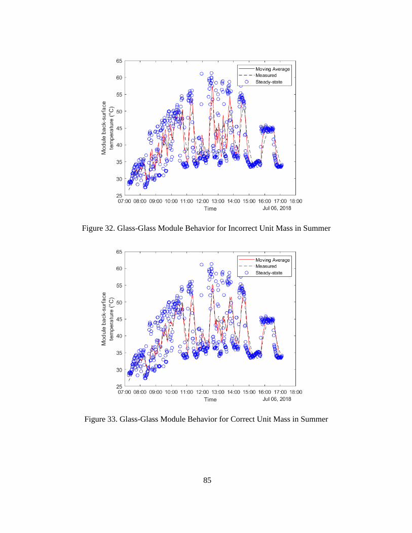
85
Figure 32. Glass-Glass Module Behavior for Incorrect Unit Mass in Summer
Figure 33. Glass-Glass Module Behavior for Correct Unit Mass in Summer

86
The incorrect unit mass calculations show clear examples of the model not matching the
shape of the measured temperature curve as a result of incorrect weighting calculations
from the incorrect unit mass value. Comparing the two Figures reveals that using accurate
unit mass calculations allows for more accurate prediction of the module temperature
peaks and thermal ramp rates for intermittent conditions. This shows that the unit mass is
truly an important parameter for the moving-average model and that it is crucial to
calculating the correct ramp rate of module temperature during times of intermittency.
4.6 Histogram Analysis
In addition to analyzing representative days in order to analyze the benefits of the
moving-average temperature model, histogram analysis was performed to identify trends
in the modeling residuals for the different climate conditions of the measured module
temperatures. These histograms were formed by taking the residuals from annual datasets
for each PV array location and binning the residuals (measured temperature – modeled
temperature) into 0.1°C bins that were then plotted as a histogram plot, with each residual
bin being plotted as a bar whose height represents the number of instances in which the
residual was within said temperature bin. This histogram analysis is shown for the
moving-average model residuals of the glass-backsheet modules for each of the four PV
array site in Figures 34 - 37.

87
Figure 34. Histogram Analysis for Albuquerque Model Fit
Figure 35. Histogram Analysis for Orlando Model Fit
Figure 36. Histogram Analysis for Las Vegas Model Fit

88
Figure 37. Histogram Analysis for Vermont Model Fit
Analysis of these Figures shows the temperature residual bin that occurs most often is
closest to 0°C for the Orlando and Williston, VT datasets. For each PV array site, the
histograms show that the moving-average temperature predictions are most often within
2°C of the measured temperatures. Visual inspection of each histogram reveals that there
is a degree of over-prediction bias across the model residuals for most of the different
climates, which is also shown by the negative MBE values in Table 5 for most of the PV
array sites. This inherent overprediction bias may be a result of the limiting nature of the
model’s reliance on the steady-state temperature predictions.
4.7 Significance of the Work
The future acceptance of the moving-average model into overall PV performance models
used throughout the industry will be dependent on its ability to improve the overall
modeling accuracy of the power generation. Evaluating how the improvements in
temperature accuracy impact the ability to accurately predict PV performance on a utility
scale requires consideration of the temperature coefficients that are reported on PV
module spec sheets and used in PV performance modeling equations [4], [18]. For an

89
assumed PV power temperature coefficient of -0.4%/°C, the expected improvements in
accuracy for each of the different PV array sites are shown in Table 8 as a percentage of
the actual annual performance found from measured PV array data. The values in this
Table are found from a simple product of the constant temperature coefficient and the
differences in model MAE between the moving-average model and steady-state model
residuals. The results in Table 8 show power performance improvements similar to that
reported for the Hayes and Ngan transient thermal model, which would show accuracy
improvement in the range of 0.08%-0.8% [14]. This shows that the moving-average
model can improve PV performance modeling accuracy to the same degree as previous
transient thermal models without adding much modeling complexity to the module
temperature calculations.
Table 8. Improvement in PV Performance Modeling Accuracy for thermal Accuracy
Improvements of Moving-Average Model
Albuquerque Orlando Vermont Las Vegas
MAE (Moving Average
- Steady-state) 0.72 1.45 0.66 0.4
Energy Accuracy
Improvement 0.29% 0.58% 0.26% 0.16%

90
CHAPTER 5
CONCLUSIONS
This thesis work has detailed the development and validation of a new approach to the
transient thermal modeling of PV module back-surface temperature. The importance of
accounting for dynamic thermal behavior of PV modules at fine temporal resolution
increases as the need for consideration of factors such as energy storage and inverter
clipping models increases. Previous attempts at these types of transient thermal models
have required numerous input parameters that are not easy to obtain for a given PV array
site. The moving-average models presented here differs from these models in that it
requires only the module mass and surface area as additional input parameters to those
environmental variables used in most steady-state temperature prediction models. This
model simplicity is achieved through development based on FEA heat transfer
simulations that revealed exponential temperature changes for the PV module that were
functions of the wind speed and unit mass of the module.
The ultimate transient thermal model resulting from this work is an exponentially
weighted moving-average of steady-state model temperature predictions within 20
minutes back in time from the time step in question. Applying the moving-average filter
to steady-state models shows decreased variability in the temperature predictions,
especially during times of rapidly changing irradiance. The model also improves upon the
accuracy of the Sandia steady-state thermal model, with improvement in the Mean
Absolute Error for 1-minute annual datasets range between 0.4°C for areas with little
solar intermittency to 1.45°C for more tropical locations characterized by intermittency in
irradiance. These improvements can lead to performance modeling accuracy

91
improvements between 0.16% to 0.58%. The moving-average model ultimately offers a
new technique for transient thermal modeling that is easier to include in PV industry
modeling practices while also being far less computationally complex than previous
attempts at transient thermal modeling.
5.1 Future Work
The moving-average model described in this thesis offers a new approach to transient
thermal modeling of PV back-surface temperatures. As the model was based on the
proven accuracy of existing steady-state models during times of low solar intermittency,
the optimum fit of the moving-average model predictions to measured temperature data is
dependent on the accuracy of these steady-state models. This means that improving the
moving-average model accuracy beyond that presented in this thesis may require
improvement of the steady-state models used in the calculation. Improving upon the
current state of steady-state thermal modeling requires investigation into inherent bias
due to environmental variables that are not currently being considered as part of the
steady-state approximations. As most steady-state models do not account for the long
wave radiation between the module and its environment, consideration of variables such
as the atmospheric sky temperature, wind direction, or humidity content of the air may
reveal trends in modeling inaccuracy. Additional considerations of the spectral content of
the irradiance may also need to be considered to gain a better understanding of the
fluctuation of module temperature as a function of the wavelength of incident light rays.
Preliminary investigation into bias error due to these variables did not reveal any clear
trends in the modeling accuracy, but further research into these models could result in
more accurate steady-state representations of module back-surface temperature.

92
Further additional work that would advance the moving-average model as it is currently
constructed would require more detailed FEA analysis or even more advanced simulation
techniques to better inform the weighting parameter of the model. Currently, the FEA
used in the model development is based on a glass sheet of varying thickness to simulate
a simplified version of the PV module’s thermal mass. Modeling the individual layers of
different types of PV modules would theoretically allow for more accuracy in the
simulated module back-surface temperatures as compared to measured module
temperatures. This would require research into the expected thermal properties for
module materials that make up components such as the solar glass, encapsulant material,
solar cells, and backsheet. There has been research into the thermal properties of these
materials [41], [42], and further development of the FEA modeling based on this research
may lead to a more conclusive understanding of different PV module types. The benefits
of such analysis and how they should be weighed against the additional modeling
complexity and specifications of each material for a variety of different module
configurations would have to be evaluated to determine the extent to which further
analysis would benefit the PV industry.
93
REFERENCES
[1] K. Mertens, Photovoltaics: Fundamentals, Technology, and Practice. Wiley, 2014.
[2] J. Good and J. X. Johnson, “Impact of inverter loading ratio on solar photovoltaic
system performance,” Appl. Energy, vol. 177, pp. 475–486, 2016, doi:
10.1016/j.apenergy.2016.05.134.
[3] M. J. Reno, M. Lave, J. E. Quiroz, R. J. Broderick, and S. N. Laboratories, “PV
Ramp Rate Smoothing Using Energy Storage to Mitigate Increased Voltage
Regulator Tapping,” Sandia Nat. Lab., Albuquerque, NM, USA, Rep. SAND2016-
5509.
[4] D. L. King, J. A. Kratochvil, and W. E. Boyson, “Photovoltaic Array Performance
Model,” Sandia Nat. Lab., Albuquerque, NM, USA, Rep. SAND2004-3535, Aug.
2004.
[5] D. Faiman, “Assessing the Outdoor Operating Temperature of Photovoltaic
Modules,” Prog. Photovoltaics Res. Appl., vol. 16, pp. 307–315, 2008, doi:
10.1002/pip.
[6] W. A. K. Al-Maliki, F. Alobaid, V. Kez, and B. Epple, “Modelling and dynamic
simulation of a parabolic trough power plant,” J. Process Control, vol. 39, 2016,
doi: 10.1016/j.jprocont.2016.01.002.
[7] J. M. Servant, "Calculation of the Cell Temperature for Photovoltaic Modules
From Climatic Data," INTERSOL 85: Proc. of the Ninth Biennial Congress of The
Internat. Solar Energy Society, vol. 3, pp. 1640-1643, 1986.
[8] S. C. W. Krauter, “Development of an integrated solar home system,” Sol. Energy
Mater. Sol. Cells, vol. 82, no. 1–2, pp. 119–130, 2004, doi:
10.1016/j.solmat.2004.01.010.
[9] T. Nordmann and L. Clavadetscher, “Understanding temperature effects on PV
system performance,” Proc. 3rd World Conf. Photovolt. Energy Convers., vol. C,
pp. 2243–2246, 2003.
[10] J. A. Duffie and W. A. Beckman, Solar Engineering of Thermal Processes, 4th ed.
Wiley, 2013.
[11] A. D. Jones and C. P. Underwood, “A Thermal Model For Photovoltaic Systems,”
Sol. Energy, vol. 70, no. 4, pp. 349–359, 2001.
[12] D. T. Lobera and S. Valkealahti, “Dynamic thermal model of solar PV systems
under varying climatic conditions,” Sol. Energy, vol. 93, pp. 183–194, 2013, doi:

94
10.1016/j.solener.2013.03.028.
[13] A. Luketa-hanlin and J. S. Stein, “Improvement and Validation of a Transient
Model To Predict Photovoltaic Module Temperature,” Sandia Nat. Lab.,
Albuquerque, NM, USA, Rep. SAND2012-5509, pp. 1–7, 2012.
[14] W. Hayes and L. Ngan, “A Time-Dependent Model for CdTe PV Module
Temperature in Utility-Scale Systems,” IEEE J. Photovoltaics, vol. 5, no. 1, pp.
238–242, 2015, doi: 10.1109/JPHOTOV.2014.2361653.
[15] “PV Education: Effect of Temperature.” PV Education. [Online]. Available:
https://www.pveducation.org/pvcdrom/solar-cell-operation/effect-of-temperature.
[16] E. Skoplaki and J. A. Palyvos, “On the temperature dependence of photovoltaic
module electrical performance : A review of efficiency / power correlations,” Sol.
Energy, vol. 83, no. 5, pp. 614–624, 2009, doi: 10.1016/j.solener.2008.10.008.
[17] A. Q. Malik and S. J. B. H. Damit, “Outdoor testing of single crystal silicon solar
cells,” Renew. Energy, vol. 28, no. 9, pp. 1433–1445, 2003, doi: 10.1016/S0960-
1481(02)00255-0.
[18] A. Mermoud and B. Wittmer, “PVSYST6,” no. May. PVSYST, Switzerland, 2017.
[19] “PVsyst Cell Temperature Model,” PV Performance Modeling Collaborative.
[Online]. Available: https://pvpmc.sandia.gov/modeling-steps/2-dc-module-iv/cell-
temperature/pvsyst-cell-temperature-model/. [Accessed: 03-Oct-2020].
[20] Terrestrial photovoltaic (PV) modules - Design qualification and type approval.
IEC 61215-2:2016, 2016.
[21] M. Muller, B. Marion and J. Rodriguez, "Evaluating the IEC 61215 Ed.3 NMOT
procedure against the existing NOCT procedure with PV modules in a side-by-side
configuration," 2012 38th IEEE Photovoltaic Specialists Conference, Austin, TX,
2012, pp. 697-702.
[22] C. Hansen, J. S. Stein, and D. Riley, “Effect of Time Scale on Analysis of PV
System Performance,” Sandia Nat. Lab.,Albuquerque, NM, USA, Rep.
SAND2012-1099, Feb. 2012.
[23] S. Armstrong and W. G. Hurley, “A thermal model for photovoltaic panels under
varying atmospheric conditions,” Appl. Therm. Eng., vol. 30, no. 11–12, pp. 1488–
1495, 2010, doi: 10.1016/j.applthermaleng.2010.03.012.
[24] K. Sayed, M. Abdel-Salam, M. Ahmed, and A. A. Ahmed, “Electro-thermal
modeling of solar photovoltaic arrays,” ASME 2011 Int. Mech. Eng. Congr. Expo.
95
IMECE 2011, vol. 4, no. PARTS A AND B, pp. 1143–1149, 2011, doi:
10.1115/imece2011-62541.
[25] S. Ransome and P. Funtan, “Why Hourly Averaged Measurement Data Is
Insufficient To Model PV System Performance Accurately,” presented at the 20th
European Photovoltaic Solar Energy Conference, 2005.
[26] Y. Lee and A. A. O. Tay, “Finite element thermal analysis of a solar photovoltaic
module,” Energy Procedia, vol. 15, no. 2011, pp. 413–420, 2012, doi:
10.1016/j.egypro.2012.02.050.
[27] Dassault Systemes Solidworks Corporation. Solidworks 2017 [Online]. Available:
www.solidworks.com.
[28] Y. Cengel and A. Ghajar, Heat and Mass Transfer: Fundamentals and
Applications, 5th ed. New York: McGraw-Hill Eduction, 2014.
[29] J. P. Holman, Heat Transfer, 10th ed. London: McGraw-Hill, 2010.
[30] Matlab and Simulink, “Nearest Neighbor, Bilinear, and Bicubic Interpolation
Methods,” The MathWorks, Inc., 2018. [Online]. Available:
https://www.mathworks.com/help/vision/ug/interpolation-methods.html.
[31] J. F. Manwell, Wind Energy Explained: Theory, Design, and Application, 2nd ed.
Wiley, 2003.
[32] W. Holmgren, C. Hansen, and M. Mikofski, “pvlib python: a python package for
modeling solar energy systems,” J. Open Source Softw., vol. 3, no. 29, p. 884,
2018.
[33] W. McKinney, “Data Structures for Statistical Computing in Python,” in
Proceedings of the 9th Python in Science Conference, 2010, vol. 9, pp. 62–72, doi:
10.3828/ajfs.41.3.62.
[34] S. Van Der Walt, S. C. Colbert, and G. Varoquaux, “The NumPy array: A
structure for efficient numerical computation,” Comput. Sci. Eng., vol. 13, no. 2,
pp. 22–30, 2011, doi: 10.1109/MCSE.2011.37.
[35] M. J. Reno and C. W. Hansen, “Identification of periods of clear sky irradiance in
time series of GHI measurements,” Renew. Energy, vol. 90, pp. 520–531, 2016,
doi: 10.1016/j.renene.2015.12.031.
[36] P. Ineichen and R. Perez, “A new airmass independent formulation for the linke
turbidity coefficient,” Sol. Energy, vol. 73, no. 3, pp. 151–157, 2002, doi:
10.1016/S0038-092X(02)00045-2.

96
[37] F. Linke, “Transmissions-Koeffizient und Trübungsfaktor,” Beitr. Phys. Atmos.,
no. 10, pp. 91–103, 1922.
[38] “Suniva Optimus ® Series Monocrystalline Solar Modules Optimus Series : Opt
72 Cell Modules.” Suniva. Available: https://www.solaris-
shop.com/content/OPT270%20Specs.pdf.
[39] Matlab and Simulink, “cdfplot: Empirical cumulative distribution function (cdf)
plot,” The MathWorks, Inc., 2018. [Online]. Available:
https://www.mathworks.com/help/stats/cdfplot.html.
[40] A. Botchkarev, “Performance Metrics (Error Measures) in Machine Learning
Regression, Forecasting and Prognostics: Properties and Typology.” Ryerson
University, Toronto, pp. 1–37, 2018.
[41] T. J. Silverman et al., “Reducing Operating Temperature in Photovoltaic
Modules,” IEEE J. Photovoltaics, vol. 8, no. 2, pp. 532–540, 2018.
[42] J. Oh et al., “Reduction of PV module temperature using thermally conductive
backsheets,” IEEE J. Photovoltaics, vol. 8, no. 5, pp. 1160–1167, 2018, doi:
10.1109/JPHOTOV.2018.2841511.

97
APPENDIX A
MOVING-AVERAGE MODEL OPEN-SOURCE CODE

98
function [T_MA_module] = pvl_ma_temp(Time, Tmodule, windspeed, m_u, varargin)
% PVL_MA_TEMP Estimate module temperature from WIND SPEED, MODULE UNIT
% MASS, PVL_SAPMCELLTEMP
%
% Syntax
% T_MA_module = pvl_ma_temp(Time, Tmodule, windspeed, m_u, deltaT, varargin)
%
% Description
% Estimate module temperatures per the transient moving-average
% temperature model (IEEE JPV, 2020), when given the 2-meter wind speed,
% module mass per unit area, SAPM temperature predictions, and bilinear
% interpolation coefficients (optional)
%
% Inputs
% Time is a struct with the following elements, note that all elements
% can be column vectors, but they must all be the same length. Time is
% entered as a struct which must include a value for the offset from
% UTC. Time is absolutely specified by the date, time, and the number
% of hours of offset from that date and time to UTC. For example, if
% you live in Boston, USA, and your data is timestamped in local standard
% time, your UTC offset should be -5.
%
% Time.year = The year in the gregorian calendar
% Time.month = the month of the year (January = 1 to December = 12)
% Time.day = the day of the month
% Time.hour = the hour of the day
% Time.minute = the minute of the hour
% Time.second = the second of the minute
% Time.UTCOffset = the UTC offset code, using the convention
% that a positive UTC offset is for time zones east of the prime meridian
% (e.g. EST = -5)
% Tmodule - A column vector of module back temperature in degrees C.
% windspeed - Wind speed in m/s measured at a height of 2 meters. windspeed
must
% be a scalar or a vector of the same size as E and Tamb. Must be >=0;
% m_u - a scalar unit mass value of the module being analyzed in kg/m^2.
% Must be >= 0;
% a - optional parameter that is used as bilinear interpolation
% coefficients to determine the moving-averge weighting function for
% windspeed and m_u; Default values from publication used if left blank
%
%
% Outputs
% T_MA_module - A column vector of module back temperature in degrees C.
%
% References
% [1] Prilliman, M. et al, 2020, "Transient Weighted Moving Average Model
% of Photovoltaic Module Back-Surface Temperature". Publication pending
%
% See also PVL_SAPMCELLTEMP
%
p = inputParser;
p.addRequired('Time',@isstruct);
p.addRequired('Tmodule',@isnumeric);
p.addRequired('windspeed',@(x) all(isnumeric(x) & isvector(x) & x>=0));
p.addRequired('m_u',@(x) all(isvector(x) & x>=0));
p.addOptional('a',[.0046; 4.5537e-4; -2.2586e-4; -1.5661e-5],@(x)
all(isnumeric(x) & numel(x)==4 & isvector(x)));
p.parse(Time,Tmodule,windspeed,m_u,varargin{:});

99
Y = Time.year; %datenum year data
M = Time.month; %datenum month data
D = Time.day; %datenum day data
h = Time.hour; %datenum hour data
m = Time.minute; %datenum minute data
s = Time.second; %datenum second data
Time = datenum(Y,M,D,h,m,s)*86400; %Time struct conveted to datenum format
a = p.Results.a; % load up values for a that were approved by the parser
%Check for monotonically incorrect datenums
if any(Time(2:end) - Time(1:end-1) < 0)
error('Times are not monotonically increasing. Exiting function')
end
a0 = a(1); %coefficients used to calculate P based on bilinear interpolation
a1 = a(2);
a2 = a(3);
a3 = a(4);
% Calculate the P values for each time step. Since the unit mass of modules
% is unlikely to change over time, we expect P to only vary due to wind
% speed changes.
P = a0+a1*windspeed+a2*m_u+a3*windspeed*m_u; %Power parameter used to determine
weights
T_MA_module = nan(size(Tmodule)); %Preallocate size of moving average model for
speed
WindowLength = 20 * 60; %Assumed window size of 1200 seconds (20 minutes)
I_B = 1; %Initialize Back Indice variable to 1
T_MA_module(1) = Tmodule(1); %First entry of moving average model always the
same as steady state model
for cntr1 = 2:length(Time)
I_F = cntr1-1; % move the front index up to the
deltaT_I_F = Time(cntr1) - Time(I_F);
% If the time difference between the current time and the most recent
% time is larger than the window length, then set the model temperature
% to the steady state temperature.
if deltaT_I_F > WindowLength
T_MA_module(cntr1) = SS(cntr1);
% If the time difference between the current time and the most recent
% time is smaller than or equal to the window length...
else
% Increment the back index until the time of the back index is less
% than or equal to the window length, as long as the back index is
% less than the front index.
while((Time(cntr1) - Time(I_B)) > (WindowLength) && (I_B<I_F))
I_B = I_B+1;
end
% Find a vector of the number of seconds backward for each
% measurement within the Window
TimeBack = (Time(cntr1) - Time(I_B:I_F));
% Find a vector of the steady state temperature predictions for
% each measurement within the window

100
TempsInWindow = Tmodule(I_B:I_F);
% Determine the weights and relative weights for each time step
% within the window
Weight = exp(-P(cntr1).*TimeBack);
Rel_weight = Weight./sum(Weight);
% Find the moving-average temperature prediction for the current
% time step.
T_MA_module(cntr1) = (TempsInWindow.') * Rel_weight;
end
end
end

101
APPENDIX B
MODEL VALIDATION SOURCE CODE

102
%% Moving Average model validation with plots and analysis of sky temperature,
wind direction, etc. bias
% -Load in field data from specified site, filter out missing or incorrect
% data, filter out for high AOI or low elevation angle,
% -Calculate input parameters such as steady-state model approximations for
% input to MA model
% -Run MA model for remaining data
% -Evaluate improvements in modeling accuracy numerically (RMSE)
% -Plot results of moving-average, SS models to evaluate model fit to
% measured data
% -Plot hourly, daily dependenices on wind direction, sky temperature,
% other neglected environmental parameters
clear all
% close all
%% Load in measured data from listed systems
% Canadian-Hanwha system (ABQ)%
load('Canadian_system_full.mat'); %1 year dataset (2018-5-27:2019-5-27)
GridData = Canadian_system_full;
load('Can_system_coeff_final.mat'); %Canadian Solar module optimized SS coeff
m_u = 18.2/(1.650*.992); %Canadian 275P spec sheet (CP strings)
a_new = -3.4432;
b_new = -.0462;
UTC = -7;
% or
% % load('Han_system_coeff_final.mat'); %Hanwha module optimized SS coeff
Location.latitude = 35.054;
Location.longitude = -106.539;
Location.altitude = 1609;
% Panasonic-LG system(ABQ)
% load('Pan_system_full.mat'); %1 year dataset (2018-5-27:2019-5-27)
% GridData = Pan_system_full;
% % % % %GridData = QueryPVGrid('','2018-05-27','2019-05-27');
% load('Pan_system_coeff_final.mat'); %Panasonic module optimized SS coeff
% % % % or
% load('LG_system_coeff.mat'); %LG module optimized SS coeff
% m_u = 18/(1.686*1.016); %LG module
%Prism systems
% load('Prism_system_full.mat'); % 1 year dataset (2018-5-27:2019-5-27)
% GridData = Prism_system_full;
% load('Prism_system_coeff_final.mat'); %Prism module optimized SS coeff
% a_new = -3.5893;
% b_new = -.0364;
% m_u = 28.9/(1.695*.984); %kg/m2 Prism Bi-60 343
% %Stion systems
% load('Stion_system_full.mat'); % 1 year dataset (2018-5-27:2019-5-27)
% GridData = Stion_system_full;
% load('Stion_opt_coeff.mat'); % Stion module optimized SS coeff
% m_u = 15/(1.650*.650); %frameless STL-140 (thin-film)
% %
csvwrite('Stion_system_full.csv',table2array(GridData(:,[25,34,35,61,62,63])));
% %or
% m_u = 16.8/(1.656*.656); %framed STO-140 (thin-film)
%Canadian system data interval test
% load('Can_system_datainterval_test.mat');
% GridData_2min = Can_system_full_2min;
% GridData_3min = Can_system_full_3min;
% GridData_4min = Can_system_full_4min;
% GridData_5min = Can_system_full_5min;

103
% GridData_7min = Can_system_full_7min;
% GridData_10min = Can_system_full_10min;
% load('Can_system_coeff_final.mat'); %Canadian Solar module optimized SS coeff
%Florida Baseline System
% load('FSEC_system.mat');
% GridData = FSEC_system_data;
% load('FSEC_system_coeff.mat');
% a_new = -3.4064;
% b_new = -.0313;
% Location.latitude = 28.3875;
% Location.longitude = -80.7560;
% Location.altitude = 25;
% UTC = -5;
%Vermont Baseline System
% load('IBMW_system.mat');
% GridData = IBMW_system_data;
% load('Vermont_system_coeff.mat');
% a_new = -3.4474;
% b_new = -.0333;
% m_u = 11.0; %Suniva OPT270
% Location.latitude = 44.4454;
% Location.longitude = -73.0992;
% Location.altitude = 184;
% UTC = -5;
%Las Vegas Baseline System
% load('LVRM_system.mat');
% GridData = LVRM_system_data;
% load('LVRM_system_coeff_final.mat');
% a_new = -3.5297;
% b_new = -.0416;
% Location.latitude = 36.1699;
% Location.longitude = -115.1398;
% Location.altitude = 610;
% UTC = -8;
%% Filter for missing or impossible data
GridData =
timetable(GridData.('Time'),GridData.('POACleanRC_E_Avg'),GridData.('AmbientTem
p_Avg'),GridData.('CP1_RTD_Avg'),GridData.('Wind_Speed_Avg'),GridData.('Wind_Di
rection_Avg'),GridData.('GHI_Avg'));%,GridData.('Sys1String1I_Avg'),GridData.('
System1Vdc_Avg'));
GridData.Properties.VariableNames =
{'POACleanRC_E_Avg','AmbientTemp_Avg','CP1_RTD_Avg','Wind_Speed_Avg','Wind_Dire
ction_Avg','GHI_Avg'};%,'Sys1String1I_Avg','System1Vdc_Avg'};
GridData = rmmissing(GridData); %Removing missing data (NaNs)
POACleanRC_E_Avg_test = GridData.('POACleanRC_E_Avg'); %find missing
POACleanRC_E_Avg data
POACleanRC_E_Avg_test2 = POACleanRC_E_Avg_test(2:end);
POACleanRC_E_Avg_test = POACleanRC_E_Avg_test(1:end-1); %take off last entry to
match length
df = ((POACleanRC_E_Avg_test2 - POACleanRC_E_Avg_test) & POACleanRC_E_Avg_test
~= 0); %Identify frozen data
f = find(df==0); %find points where df = 0, POACleanRC_E_Avg ~= 0
GridData(f+1,:) = []; %Remove points where data is frozen at value of

104
AmbientTemp_Avg_test = GridData.('AmbientTemp_Avg'); %find missing
POACleanRC_E_Avg data
AmbientTemp_Avg_test2 = AmbientTemp_Avg_test(2:end);
AmbientTemp_Avg_test = AmbientTemp_Avg_test(1:end-1); %take off last entry to
match length
df = ((AmbientTemp_Avg_test2 - AmbientTemp_Avg_test)); %Identify frozen data
f = find(df==0); %find points where df = 0, POACleanRC_E_Avg ~= 0
GridData(f+1,:) = []; %Remove points where data is frozen at value of last
working measurement (logger communication error)
CP1_RTD_Avg_test = GridData.('CP1_RTD_Avg'); %find missing POACleanRC_E_Avg
data
CP1_RTD_Avg_test2 = CP1_RTD_Avg_test(2:end);
CP1_RTD_Avg_test = CP1_RTD_Avg_test(1:end-1); %take off last entry to match
length
df = ((CP1_RTD_Avg_test2 - CP1_RTD_Avg_test)); %Identify frozen data
f = find(df==0); %find points where df = 0, POACleanRC_E_Avg ~= 0
GridData(f+1,:) = []; %Remove points where data is frozen at value of last
working measurement (logger communication error)
Wind_Speed_Avg_test = GridData.('Wind_Speed_Avg'); %find missing
POACleanRC_E_Avg data
Wind_Speed_Avg_test2 = Wind_Speed_Avg_test(2:end);
Wind_Speed_Avg_test = Wind_Speed_Avg_test(1:end-1); %take off last entry to
match length
df = ((Wind_Speed_Avg_test2 - Wind_Speed_Avg_test)); %Identify frozen data
f = find(df==0); %find points where df = 0, POACleanRC_E_Avg ~= 0
GridData(f+1,:) = []; %Remov
f1 = (GridData.('AmbientTemp_Avg')<(-15)) | (GridData.('AmbientTemp_Avg')>80);
%Ambient temperature filter
GridData(f1,:) = [];
f2 = (GridData.('CP1_RTD_Avg')< (GridData.('AmbientTemp_Avg')-10)) |
(GridData.('CP1_RTD_Avg') > (GridData.('AmbientTemp_Avg')+70));
GridData(f2,:) = []; %Measured module temperature filter
f3 = (GridData.('POACleanRC_E_Avg')<0) | (GridData.('POACleanRC_E_Avg')>1500);
%measured POACleanRC_E_Avg irradiance filter
GridData(f3,:) = [];
f4 = (GridData.('Wind_Speed_Avg')<0) ; %wind speed filter
GridData(f4,:) = [];
%% Filter for solar position
%AOI > 75 excluded (most of irradiance hitting back of module)
%SunEl < 10 deg excluded (sun not over mountains in ABQ)
Time = datenum(GridData.('Time')); %convert datetime to datenum
% UTC = -8; %UTC offset (MDT)
TmStamp = pvl_maketimestruct(Time, UTC); %make time struct for conformity with
pvlib matlab
%Calculate solar position parameters to find angle of incidence
%Perform dual filter on GHI data found in clear sky detection
%Only take data with AOI < 75 and solar elevation angle > 10 (to see over
%mountains)
[SunAz, SunEl, ApparentSunEl, SolarTime]=pvl_ephemeris(TmStamp, Location);
%ephemeris function from pvlib matlab
SunZen = 90-ApparentSunEl; %Solar zenith angle is complementary to apparent
solar elevation angle
SurfTilt = Location.latitude; %Systems are at latitude tilt
SurfAz = 180; %System azimuth set to face due south (North = 0°)
AOI = pvl_getaoi(SurfTilt,SurfAz,SunZen,SunAz); %Angle of incidence between sun
and module

105
crit = find(AOI<75 & ApparentSunEl>10); %filtering criteria (measurements to
include)
% crit = find(AOI<75);
GridData = GridData(crit,:); %filter data based on criteria
Time = datenum(GridData.('Time')); %convert datetime to datenum
UTC = -7; %UTC offset (MDT)
TmStamp = pvl_maketimestruct(Time, UTC); %make time struct for conformity with
pvlib matlab
%% Parameter calculations
a_ss = -3.56; %upper limit coefficient glass/cell/polymer sheet (SAPM)
b_ss = -0.075; %wind coefficient glass/cell/polymer sheet (SAPM)
delta_T = 3; %difference between cell and back surface temperature (SAPM) degC
POACleanRC_E_Avg = GridData.('POACleanRC_E_Avg'); %separate POACleanRC_E_Avg
into single for calculation
E_0 = 1000; %correction irradiance value for different between cell and module
temperature
V_w = GridData.('Wind_Speed_Avg'); %wind speed measured at height of 2 meters
(separated into single for calculation)
wind_height = 2; %wind measured at a height of 2 m
Module_height = 10; %desired wind measurement height of 10 meters based on SS
model design
Z_0 = 0.25; %roughness length based on
WS = V_w*log(Module_height/Z_0)/log(wind_height/Z_0); %wind speed at 10 meters
for input into Sandia steady-state model
T_a = GridData.('AmbientTemp_Avg'); %ambient temperature separated into single
for calculation
%Sandia steady-state model calculation
[SNL_old_Tc, SNL_old_Tm] = pvl_sapmcelltemp(POACleanRC_E_Avg, E_0, a_ss, b_ss,
WS, T_a, delta_T); %pvlib matlab function of SAPM steady-state model
[SNL_new_Tc, SNL_new_Tm] = pvl_sapmcelltemp(POACleanRC_E_Avg, E_0, a_new,
b_new, WS, T_a, delta_T); %pvlib matlab function of SAPM steady-state model
SNL = SNL_old_Tm; %module temperature SS calculation
T_meas = (GridData.('CP1_RTD_Avg')); %Measured module temperature separated for
calculation, comparison
%% Run Moving Average Model for given unit mass, bilinear interpolation
coefficients
%bilinear interpolation coefficients
a = [.0046; 4.5537e-4; -2.2586e-4; -1.5661e-5];
% load('new_bilinearinterp.mat');
% P = a(1)+a(2)*V_w+a(3)*m_u+a(4)*V_w*m_u; %P calculated in pvl_MAmodel
%coefficient a0,a1,a2,a3 from bilinear interpolation
%%Run MA model for given inputs
T_MA = pvl_MAmodel_index(TmStamp, SNL, V_w, m_u, a); %MA model based on Sandia
SS model
%% Numerical Evaluation of Moving Average Model fit

106
RMSE_MA = sqrt(mean((T_MA(:)-T_meas(:)).^2)); %root mean square of moving
average model output to measured data
RMSE_SNL = sqrt(mean((SNL-T_meas(:)).^2)); %root mean square of steady-state
model output to measured data
RMSE_test = sqrt(mean((T_meas(:) - T_MA(:)).^2));
%mean bias (mean(Tma-Tmeas)) MA-moving average SS-steady-state
Mean_BIAS_MA= mean(T_meas - T_MA); %bias error of moving average model output
to measured data
Mean_BIAS_SNL = mean(T_meas - SNL); %bias error of steady-state model output to
measured data
%mean absolute (mean(abs(T_ma - T_meas)) MA-moving average SS-steady-state
Mean_Abs_MA = mean(abs(T_MA-T_meas)); %absolute bias error of moving average
model output to measured data
Mean_Abs_SNL = mean(abs(SNL-T_meas)); %absolute bias error of moving average
model output to measured data
R_squared_MA = 1 - sum((T_MA-T_meas).^2)/sum((T_meas - mean(T_meas)).^2); %R-
squared fit of moving average model output to measured data
R_squared_SNL = 1 - sum((SNL - T_meas).^2)/sum((T_meas - mean(T_meas)).^2); %R-
squared fit of steady-state model output to measured data
figure
h = histogram(T_meas - T_MA)
grid on
xlim([-20 20])
xlabel('Residual (Measured - Modeled) (°C)')
ylabel('Number of instances')
%% DOE Report Calendar Plot
close all
[Year Month Day] = ymd(GridData.('Time'));
Time_calendar = GridData.('Time');
hyperlink_Temp = cell(max(Month),max(Day));
hyperlink_POACleanRC_E_Avg = cell(max(Month),max(Day));
for j = 1:1:12
Month_check = Month==j;
figure
if isempty(Day(Month_check))
Day_iter = 1;
else
Day_iter = max(Day(Month_check));
end
for i = 1:1:Day_iter
if any(Day(Month_check))
subplot(6,6,i)
x = Time_calendar(Month_check & Day==i);
y1 = T_MA(Month_check & Day==i);
y2 = T_meas(Month_check & Day==i);
y3 = SNL(Month_check & Day==i);
plot(x,[y1 y2 y3])
ylim([0 75])
Disp = ['<a href="matlab:figure;plot(x,[y1 y2 y3]);ylim([0
75]);legend(''MA'',''Meas'',''SS'');">Plot Month',num2str(j),'Day',num2str(i),'
Temps</a>'];
% disp(Disp)
hyperlink_Temp(j,i) = cellstr(Disp);
else
subplot(6,6,i)
plot(0,0, 0,0, 0,0, 0,0)

107
end
end
subplot(6,6,i+1)
plot(0,0, 0,0, 0,0, 0,0)
axis off
lgd2 = legend('MA','Meas','SNL');
lgd2.FontSize = 24;
end
% for i = 1:1:max(max(Day(August)),1)
% if any(Day(August))
% subplot(6,6,i)
% x = Time_calendar(August & Day==i);
% y4 = POACleanRC_E_Avg(August & Day==i);
% plot(x,y4)
% ylim([0 1500])
% else
% end
% end
Time_calendar = GridData.('Time');
for j = 1:1:12
Month_check = Month==j;
figure
if isempty(Day(Month_check))
Day_iter = 1;
else
Day_iter = max(Day(Month_check));
end
for i = 1:1:Day_iter
if any(Day(Month_check))
subplot(6,6,i)
x = Time_calendar(Month_check & Day==i);
y1 = T_MA(Month_check & Day==i);
y2 = T_meas(Month_check & Day==i);
y3 = SNL(Month_check & Day==i);
y4 = POACleanRC_E_Avg(Month_check & Day==i);
plot(x,y4)
ylim([0 1500])
Disp = ['<a href="matlab:figure;plot(x,y4);ylim([0
1500]);legend(''POACleanRC_E_Avg'');">Plot
Month',num2str(j),'Day',num2str(i),'POACleanRC_E_Avg Irradiance</a>'];
% disp(Disp)
Disp2 = ['<a href="matlab:figure;plot(x,[y1 y2 y3]);ylim([0
75]);legend(''MA'',''Meas'',''SS'');">Plot Month',num2str(j),'Day',num2str(i),'
Temps</a>'];
hyperlink_POACleanRC_E_Avg(j,i) = cellstr(Disp);
hyperlink_Temp(j,i) = cellstr(Disp2);
else
subplot(6,6,i)
plot(0,0, 0,0, 0,0, 0,0)
end
end
subplot(6,6,i+1)
plot(0,0, 0,0, 0,0, 0,0)
axis off
lgd = legend('POACleanRC_E_Avg');

108
lgd.FontSize = 24;
end
hyper_POACleanRC_E_Avg = cell2table(hyperlink_POACleanRC_E_Avg);
hyper_Temp = cell2table(hyperlink_Temp);
hyper_POACleanRC_E_Avg.Properties.RowNames =
{'Jan','Feb','Mar','Apr','May','Jun','Jul','Aug','Sep','Oct','Nov','Dec'};
hyper_Temp.Properties.RowNames = hyper_POACleanRC_E_Avg.Properties.RowNames;
%% Separate days found from POACleanRC_E_Avg calendar plots
% Temperatures from Canadian Hanwha solar module for DOE Report
[Year Month Day] = ymd(GridData.('Time'));
Time = GridData.('Time');
Wind_Dir = GridData.('Wind_Direction_Avg');
Wind_Speed = GridData.('Wind_Speed_Avg');
%None in January
%February
Feb_Temp = [(Month==2 & Day==10), (Month==2 & Day==18), (Month==2 & Day==28)];
Feb10 = [T_MA(Feb_Temp(:,1)), T_meas(Feb_Temp(:,1)), SNL(Feb_Temp(:,1))];
%February 18 Temperatures
Feb18 = [T_MA(Feb_Temp(:,2)), T_meas(Feb_Temp(:,2)), SNL(Feb_Temp(:,2))];
%February 20 Temperatures
Feb28 = [T_MA(Feb_Temp(:,3)), T_meas(Feb_Temp(:,3)), SNL(Feb_Temp(:,3))];
%February 28 Temperatures
figure
Mean_Abs_MA_Feb18 = mean(abs(Feb18(:,2) - Feb18(:,1)));
Mean_Abs_SNL_Feb18 = mean(abs(Feb18(:,2) - Feb18(:,3)));
RMSE_MA_Feb18 = sqrt(mean((Feb18(:,2)-Feb18(:,1)).^2)); %root mean square of
moving average model output to measured data
RMSE_SNL_Feb18 = sqrt(mean((Feb18(:,2)-Feb18(:,3)).^2));
figure
plot(Time(Feb_Temp(:,2)),Feb18(:,1),'-r')
hold on
plot(Time(Feb_Temp(:,2)),Feb18(:,2),'--k')
plot(Time(Feb_Temp(:,2)),Feb18(:,3),'ob')
xlabel('Time')
ylabel({'Module back-surface'; 'temperature (°C)'})
legend('Moving Average','Measured','Steady-state','Location','Northeast');
%July
Jul_Temp = [(Month==7 & Day==5), (Month==7 & Day==6), (Month==7 & Day==8)];
Jul5 = [T_MA(Jul_Temp(:,1)), T_meas(Jul_Temp(:,1)), SNL(Jul_Temp(:,1))]; %July
5 Temperatures
Jul6 = [T_MA(Jul_Temp(:,2)), T_meas(Jul_Temp(:,2)), SNL(Jul_Temp(:,2))]; %July
6 Temperatures
Jul8 = [T_MA(Jul_Temp(:,3)), T_meas(Jul_Temp(:,3)), SNL(Jul_Temp(:,3))]; %July
8 Temperatures
Mean_Abs_MA_Jul6 = mean(abs(Jul6(:,2) - Jul6(:,1)));
Mean_Abs_SNL_Jul6 = mean(abs(Jul6(:,2) - Jul6(:,3)));
RMSE_MA_Jul6 = sqrt(mean((Jul6(:,2)-Jul6(:,1)).^2)); %root mean square of
moving average model output to measured data
RMSE_SNL_Jul6 = sqrt(mean((Jul6(:,2)-Jul6(:,3)).^2));
figure
plot(Time(Jul_Temp(:,2)),Jul6(:,1),'-r')
hold on
plot(Time(Jul_Temp(:,2)),Jul6(:,2),'--k')
plot(Time(Jul_Temp(:,2)),Jul6(:,3),'ob')
xlabel('Time')
ylabel({'Module back-surface'; 'temperature (°C)'})

109
legend('Moving Average','Measured','Steady-state','Location','Northeast');
%% RMSE for whole year
close all
[Year Month Day] = ymd(GridData.('Time'));
% Power = GridData.('System1Vdc_Avg').*GridData.('Sys1String1I_Avg');
% Power = Power*60/(1000*3600);
% Power_t = timetable(GridData.('Time'),Power);
Time = GridData.('Time');
RMSE_MA_month = zeros(12,1);
RMSE_SS_month = zeros(12,1);
POA_avg_month = zeros(12,1);
Power_month = zeros(12,1);
for m = 1:1:12
month_iter = [Month == m];
month_Time = Time(month_iter);
T_MA_month = T_MA(month_iter);
T_SS_month = SNL(month_iter);
T_meas_month = T_meas(month_iter);
RMSE_MA_month(m) = sqrt(mean((T_MA_month(:)-T_meas_month(:)).^2)); %root
mean square of moving average model output to measured data
RMSE_SS_month(m) = sqrt(mean((T_SS_month(:)-T_meas_month(:)).^2)); %
POA_avg_month(m) = mean(POACleanRC_E_Avg(month_iter));
% Power_iter = Power_t(month_iter,1);
% Power_month(m) = sum(table2array(Power_iter));
end
figure
RMSE_bar = [RMSE_MA_month RMSE_SS_month];
RMSE_bar = double(RMSE_bar);
X =
categorical({'Jan','Feb','Mar','Apr','May','Jun','Jul','Aug','Sep','Oct','Nov',
'Dec'});
X =
reordercats(X,{'Jan','Feb','Mar','Apr','May','Jun','Jul','Aug','Sep','Oct','Nov
','Dec'});
b = bar(X,RMSE_bar,'FaceColor','flat')
b(1).CData = [ones(12,1) zeros(12,1) zeros(12,1)];
b(2).CData = [zeros(12,1) zeros(12,1) ones(12,1)];
xlabel('Month')
ylabel('Average RMSE between measured and modeled data (°C)')
legend('Moving Average','Steady-state')
Recommended