Motion Tracking Algorithms for Inertial Measurement Javier Torres
Tyndall National Institute
University College Cork
Ireland 00 353 21 4904376
Brendan O’Flynn Tyndall National
Institute University College
Cork Ireland
00 353 21 4904088
Philip Angove Tyndall National
Institute University College
Cork Ireland
00 353 21 4904401
Frank Murphy Tyndall National
Institute University College
Cork Ireland
00 353 21 4904088
Cian O’ Mathuna Tyndall National
Institute University College
Cork Ireland
00 353 21 4904088
ABSTRACT In this paper, we describe the development of the software
algorithms required to interpret sensor data developed by a
wearable miniaturized wireless inertial measurement unit (IMU)
to enable tracking of movement
Traditionally, inertial tracking has involved the use of off
the shelf motion sensors in the form of an inertial measurement
unit, in combination with a GPS based receiver system for
improved accuracy. Several immediate concerns are evident when
a low cost, low power consumption, miniaturised solution is
needed in applications such as animal tracking. GPS solutions
have proven to be costly requiring an expensive satellite link &
entail power supply and size concerns when deployed on live
animals. In particular applications, GPS coverage is not available
for all application scenarios and alternative mechanisms for
motion tracking are required. IMUs cannot be used in isolation for
absolute position tracking, since an IMU calculates position
utilising a square function of time (t) where the error is
proportional to the sampling time, any errors in the output of the
sensors are therefore also multiplied by t². This typically leads to
large positional errors in operation: These issues can potentially
be addressed by using only a low cost modular IMU solution to
enable the mapping of movement if appropriate algorithms are
implemented
The goal of this paper is to present a mathematical
algorithm that enables an inertial -based tracking system to be
realized. This algorithm could then be used with GPS (GPS is
commonly used but there are other methods like triangulation)
along with a Kalman Filter algorithm providing an accurate 3-
Dimensional tracking system.
Categories and Subject Descriptors D.2.4 Algorithms, B.4.1 Data Communications Devices, E.1
Data Structures, F.2.1 Numerical Algorithms & Problems
General Terms Algorithms, Measurement, Design, Reliability, Experimentation
Keywords Wireless Inertial Measurement Unit (WIMU). Kalman Filter,
Motion Tracking, algorithms.
1. INTRODUCTION Autonomous position mapping can be realized using a
miniaturized wireless IMU with 3-axis sensor outputs indicating
acceleration, angular velocity & magnetic field. Using this
information as inputs to a system of equations representing IMU
motion, the resultant positional displacement, angular rotation &
compass orientation relative to the earth’s magnetic field, in all 3-
axes can be realized.
This positional data could for instance be utilised with GIS
mapping software to see the movement of the body either in real
time following data download, or interact directly with the
environment [1], depending on the application.
The inherent drift common in all IMU sensors can be
compensated for using an additional system as appropriate e.g. an
RFID system to give a zero (origin) datum point correction, or
another application specific zeroing mechanism (GPS,
triangulation etc.). Furthermore filtering algorithms such as
Kalman filtering [2] [3] [4] or digital filtering of the sensor
outputs can be enabled for improved accuracy.
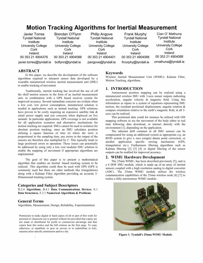
2. WIMU Hardware Development The 25mm WIMU, has been described previously [5], and is
a 6 DOF IMU module, which is made up of an array of inertial
sensors coupled with a high resolution analog to digital converter
(ADC). The 25mm WIMU module utilises the wireless
communication capabilities of the 25mm wireless node [6] [7] to
realise a fully autonomous WIMU module.
Figure 1. Tyndall's 25mm WIMU Module
Permission to make digital or hard copies of all or part of this work for
personal or classroom use is granted without fee provided that copies are
not made or distributed for profit or commercial advantage and that
copies bear this notice and the full citation on the first page. To copy
otherwise, or republish, to post on servers or to redistribute to lists,
requires prior specific permission and/or a fee.
Conference’04, Month 1–2, 2004, City, State, Country.
Copyright 2004 ACM 1-58113-000-0/00/0004…$5.00.
The wireless node has an integrated ATMEL ATMega128
[8] microcontroller for the development of customised embedded
protocol algorithms for the networking of the modules. This
feature coupled with the 2.4GHz transceiver, RF Nordic nRF2401
[9], produces a very powerful customisable wireless node.
Alternative implementations enable the Zigbee (IEEE 802.15.4)
communications in the 25mm form factor if required. The 25mm
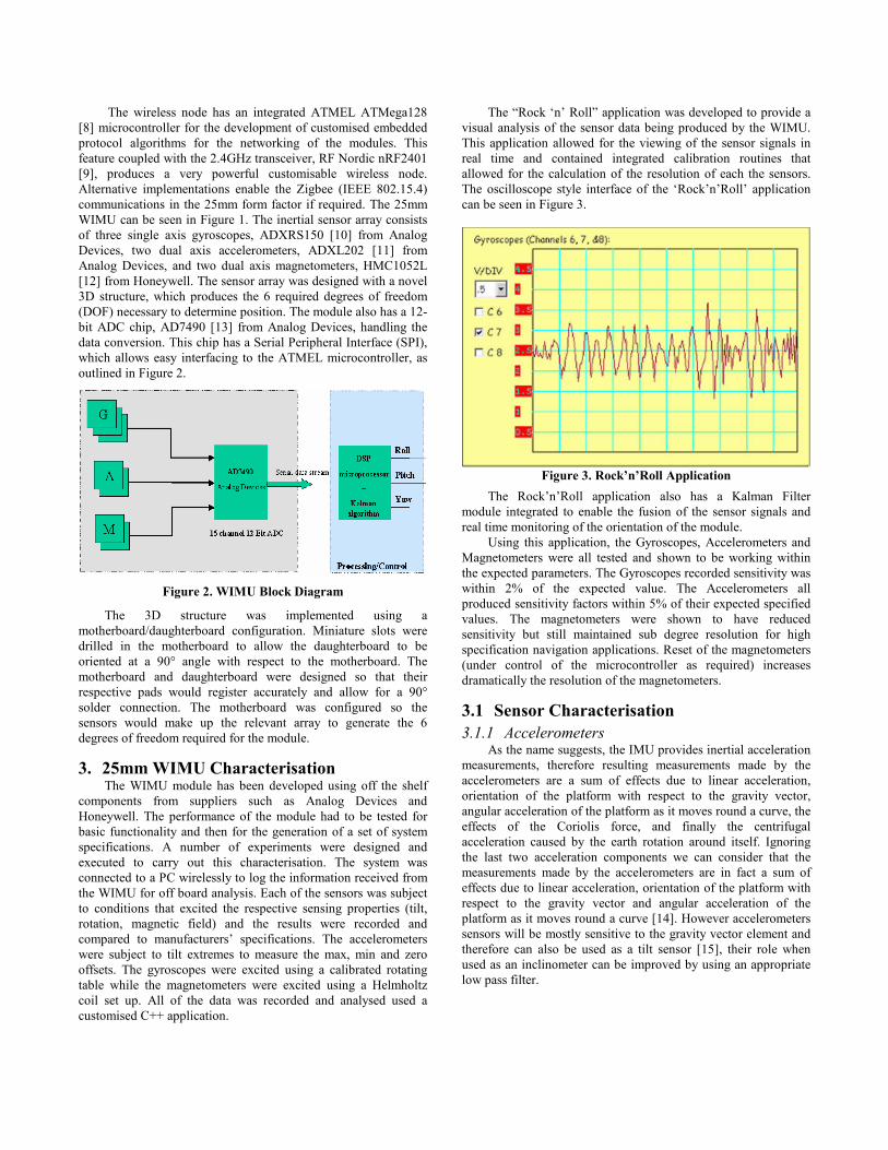
WIMU can be seen in Figure 1. The inertial sensor array consists
of three single axis gyroscopes, ADXRS150 [10] from Analog
Devices, two dual axis accelerometers, ADXL202 [11] from
Analog Devices, and two dual axis magnetometers, HMC1052L
[12] from Honeywell. The sensor array was designed with a novel
3D structure, which produces the 6 required degrees of freedom
(DOF) necessary to determine position. The module also has a 12-
bit ADC chip, AD7490 [13] from Analog Devices, handling the
data conversion. This chip has a Serial Peripheral Interface (SPI),
which allows easy interfacing to the ATMEL microcontroller, as
outlined in Figure 2.
Figure 2. WIMU Block Diagram
The 3D structure was implemented using a
motherboard/daughterboard configuration. Miniature slots were
drilled in the motherboard to allow the daughterboard to be
oriented at a 90° angle with respect to the motherboard. The
motherboard and daughterboard were designed so that their
respective pads would register accurately and allow for a 90°
solder connection. The motherboard was configured so the
sensors would make up the relevant array to generate the 6
degrees of freedom required for the module.
3. 25mm WIMU Characterisation The WIMU module has been developed using off the shelf
components from suppliers such as Analog Devices and
Honeywell. The performance of the module had to be tested for
basic functionality and then for the generation of a set of system
specifications. A number of experiments were designed and
executed to carry out this characterisation. The system was
connected to a PC wirelessly to log the information received from
the WIMU for off board analysis. Each of the sensors was subject
to conditions that excited the respective sensing properties (tilt,
rotation, magnetic field) and the results were recorded and
compared to manufacturers’ specifications. The accelerometers
were subject to tilt extremes to measure the max, min and zero
offsets. The gyroscopes were excited using a calibrated rotating
table while the magnetometers were excited using a Helmholtz
coil set up. All of the data was recorded and analysed used a
customised C++ application.
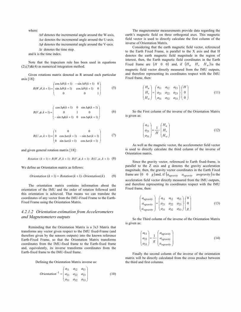
The “Rock ‘n’ Roll” application was developed to provide a
visual analysis of the sensor data being produced by the WIMU.
This application allowed for the viewing of the sensor signals in
real time and contained integrated calibration routines that
allowed for the calculation of the resolution of each the sensors.
The oscilloscope style interface of the ‘Rock’n’Roll’ application
can be seen in Figure 3.
Figure 3. Rock’n’Roll Application
The Rock’n’Roll application also has a Kalman Filter
module integrated to enable the fusion of the sensor signals and
real time monitoring of the orientation of the module.
Using this application, the Gyroscopes, Accelerometers and
Magnetometers were all tested and shown to be working within
the expected parameters. The Gyroscopes recorded sensitivity was
within 2% of the expected value. The Accelerometers all
produced sensitivity factors within 5% of their expected specified
values. The magnetometers were shown to have reduced
sensitivity but still maintained sub degree resolution for high
specification navigation applications. Reset of the magnetometers
(under control of the microcontroller as required) increases
dramatically the resolution of the magnetometers.
3.1 Sensor Characterisation
3.1.1 Accelerometers As the name suggests, the IMU provides inertial acceleration
measurements, therefore resulting measurements made by the
accelerometers are a sum of effects due to linear acceleration,
orientation of the platform with respect to the gravity vector,
angular acceleration of the platform as it moves round a curve, the
effects of the Coriolis force, and finally the centrifugal
acceleration caused by the earth rotation around itself. Ignoring
the last two acceleration components we can consider that the
measurements made by the accelerometers are in fact a sum of
effects due to linear acceleration, orientation of the platform with
respect to the gravity vector and angular acceleration of the
platform as it moves round a curve [14]. However accelerometers
sensors will be mostly sensitive to the gravity vector element and
therefore can also be used as a tilt sensor [15], their role when
used as an inclinometer can be improved by using an appropriate
low pass filter.

Figure 4: Signal output of the accelerometer with
sensitive axis in the U direction.
Figure 4 above graphically shows the signal output of the
accelerometer which has its sensitive axis in the U direction (see
Figure 8). The first segment of the wave form shows the
acceleration measured while we were changing the U axis from a
plane in which it’s parallel to the earth’s surface to a plane in
which it points toward the earth’s core and the sensor is
experiencing a force of 1g (9.81m/s2). This is the acceleration due
to tilt respect to gravity.
The second segment shows the acceleration measured with
the same motion as the first section, but with simultaneous
inclusion of dynamic acceleration.
3.1.2 Gyroscopes Gyroscopes are angular velocity sensing devices. They
provide the angular velocity around the three orthogonal axes.
The first time integration of the angular velocity leads to the Euler
angles that are necessary to describe the orientation of the IMU.
The Euler angles are usually given in aeronautical term as Pitch,
Roll and Yaw (See Figure 8), where: Pitch is the rotation around
the lateral (V) axis, Roll around the longitudinal (U) axis and
Yaw around the perpendicular (W) one.
Figure 5. Gyroscopes’ outputs
3.1.3 Magnetometers The magnetometers integrated into the IMU system measure
the earth magnetic field on three orthogonal axes. Figure 6 shows
the magnetometer output in the West direction (see Figure 7)
while we were changing its orientation from north to south.
The Earth’s magnetic field intensity is about 0.5 to 0.6
Gauss, it is approximated with a dipole model and has a
component parallel to the Earth’s surface that always pointing
toward magnetic north and is used to determine compass
direction.
For establishing device orientation, the key components of
the magnetometers’ sensor data are a) parallel to the earth’s
surface and b) in the direction of the earth’s magnetic north.
These vectors can be used to estimate the direction cosine matrix
(it will be called Orientation Matrix from now on) defined in
section 4.1.
The end result of these calculations is an orientation
estimation referenced with respect to the magnetic north, which
differs from geographic north, by about 5 degrees in geographic
locations found in Ireland. Geographic north is located at the
earth’s rotational axis and is referenced by the meridian lines
found on maps. At different locations around the globe, magnetic
and geographic north can differ by ±25 degrees. This difference is
called the declination angle and can be determined from a lookup
table based on the geographic location.
Figure 6: Magnetometers outputs
Generally it is possible to obtain the orientation of the IMU
with high accuracy by fusing Gyroscope, Accelerometer, and
Magnetometer signals via Kalman Filtering [16,17].
In this case, the accelerometers are used as a tilt sensor,
under this approach is useful to use an appropriate low pass Filter
that make the accelerometers signal more sensitive to gravity [18]
and the magnetometers are used as a compass.

4. Inertial Systems Equations.
4.1 Frames Measurements made directly from the IMU are referenced
with respect to the IMU sensors axes, which are fixed by the
physical orientation of the sensors. These axes (Figure 7) are
called the IMU-Fixed Frame and all the sensor outputs are
referenced to this frame.
Figure 7. WIMU gyro, accelerometer and magnetometer layout
and IMU-Fixed Frame.
To enable the tracking of positioning and orientation, we
need to reference the data to a known origin (reference frame. To
achieve this we use the Earth-Fixed Frame (Figure 8) that is
defined with its X-axis parallel to the Earth’s surface and pointing
toward the Earth magnetic North, its Z-axis parallel to the gravity
vector and therefore perpendicular to the Earth’s surface and Y-
axis will be the cross product between the Z and X axes.
Figure 8. Earth Fixed Frame.
The Orientation Matrix is a 3x3 Matrix that transforms any
vector given respect to the IMU fixed-Frame (and therefore given
by the sensors outputs) into the known reference Earth-Fixed
Frame.
4.2 Algorithms Development for inertial
(IMU)-based tracking system The 3-axis acceleration & angular velocity sensor output
values can be combined in a non-linear matrix equation to give
both position & orientation information.
The system can be visualized by using a fixed frame of
reference for position measurement (x, y, z): The Earth-Fixed
Frame and utilizing a moving non-inertial frame (u, v, w): IMU-
Fixed Frame with its axes parallel to the IMU sensors axes (see
Figures 7, 8 and 9)
Figure 9. Moving and Reference frames
4.2.1 Orientation Estimation Calculations The Orientation of the IMU will have two sources of
estimation: gyroscopes outputs and the outputs from the
accelerometers and magnetometers. Gyroscopes cannot be used in
isolation for obtaining absolute Orientation because of the drift
associated with their readings. Magnetometers & accelerometers
lead to orientation estimation with long-term stability but short-
term occasional inaccuracy due to the presence of ferromagnetic
materials or other magnetic fields (different to the earth’s
magnetic field) and due to linear and rotational accelerations that
disturb the orientation estimation.
Thus we can combine the advantage of the short-term
precision of Gyroscopes and the long-term stability of
Accelerometers and Magnetometers via a Kalman Filter.
4.2.1.1 Orientation estimation from gyroscope
outputs Every time step we are able to know the Euler angles θφα ,, ,
we can keep the order of rotation and follow it every time step as
follows:
Definition of Angles
2
)()1()1(
kktk
θθθ
&& ++⋅∆=+∆ (Yaw) (2)
2
)()1()1(
kktk
φφφ
&& ++⋅∆=+∆ (Pitch) (3)
2
)()1()1(
kktk
ααα
&& ++⋅∆=+∆ (Roll) (4)
where:
θ∆ denotes the incremental angle around the W-axis,
α∆ denotes the incremental angle around the U-axis.
φ∆ denotes the incremental angle around the V-axis.
t∆ denotes the time step.
and k is the time index.
Note that the trapezium rule has been used in equations
(2),(3)&(4) as numerical integration method.
Given rotations matrix denoted as R around each particular
axis [18]:
+∆+∆
+∆−+∆
=+
100
0)1(cos)1(sin
0)1(sin)1(cos
)1,,( kk
kk
kWR θθθθ
θ (5)
+∆+∆−
+∆+∆
=+
)1(cos0)1(sin
010
)1(sin0)1(cos
)1,,(
kk
kk
kVR
φφ
φφφ (6)
+∆+∆
+∆−+∆=+
)1(cos)1(sin0
)1(sin)1(cos0
001
)1,,(
kk
kkkUR
ααααα (7)
and given general rotation matrix [18]:
)1,,()1,,()1,,()1( +⋅+⋅+=+ kURkVRkWRkRotation αφθ (8)
We define an Orientation matrix as follows:
)()1()1( knOrientatiokRotationknOrientatio ⋅+=+ (9)
The orientation matrix contains information about the
orientation of the IMU and the order of rotation followed until
this orientation is achieved. That means we can translate the
coordinates of any vector from the IMU-Fixed Frame to the Earth-
Fixed Frame using the Orientation Matrix.
4.2.1.2 Orientation estimation from Accelerometers
and Magnetometers outputs
Reminding that the Orientation Matrix is a 3x3 Matrix that
transforms any vector given respect to the IMU fixed-Frame (and
therefore given by the sensors outputs) into the known reference
Earth-Fixed Frame, so that the Orientation Matrix transforms
coordinates from the IMU-fixed frame to the Earth-fixed frame
and, equivalently, its inverse transforms coordinates from the
Earth-fixed frame to the IMU-fixed frame.
Defining the Orientation Matrix inverse as:
=−
333231
232221
1312111
aaa
aaa
aaa
nOrientatio (10)
The magnetometer measurements provide data regarding the
earth’s magnetic field on three orthogonal axes. This magnetic
field vector is used to directly calculate the first column of the
inverse of Orientation Matrix.
Considering that the earth magnetic field vector, referenced
to the Earth Fixed Frame, is parallel to the X axis and that H
denotes the earth magnetic field magnitude in the region of
interest, then, the Earth magnetic field coordinates in the Earth
Fixed frame are ( )00H and, if ( )wvu HHH is the
magnetic field vector directly measured from the IMU outputs,
and therefore representing its coordinates respect with the IMU
Fixed frame, then:
⋅
=
0
0
333231
232221
131211 H
aaa
aaa
aaa
H
H
H
w
v
u
(11)
So the First column of the inverse of the Orientation Matrix
is given as:
⋅=
w
v
u
H
H
H
Ha
a
a1
31
21
11
(12)
As well as the magnetic vector, the accelerometer field vector
is used to directly calculate the third column of the inverse of
Orientation matrix.
Since the gravity vector, referenced to Earth fixed-frame, is
parallel to the Z axis and g denotes the gravity acceleration
magnitude, then, the gravity vector coordinates in the Earth Fixed
frame are ( )g00 and, if ( )awgravityaa vgravityugravity is the
acceleration field vector directly measured from the IMU outputs,
and therefore representing its coordinates respect with the IMU
Fixed frame, then:
⋅
=
gaaa
aaa
aaa
a
a
a
wgravity
vgravity
ugravity
0
0
333231
232221
131211
(13)
So the Third column of the inverse of the Orientation Matrix
is given as:
⋅=
wgravity
vgravity
ugravity
a
a
a
ga
a
a1
33
23
13
(14)
Finally the second column of the inverse of the orientation
matrix will be directly calculated from the cross product between
the third and first columns.
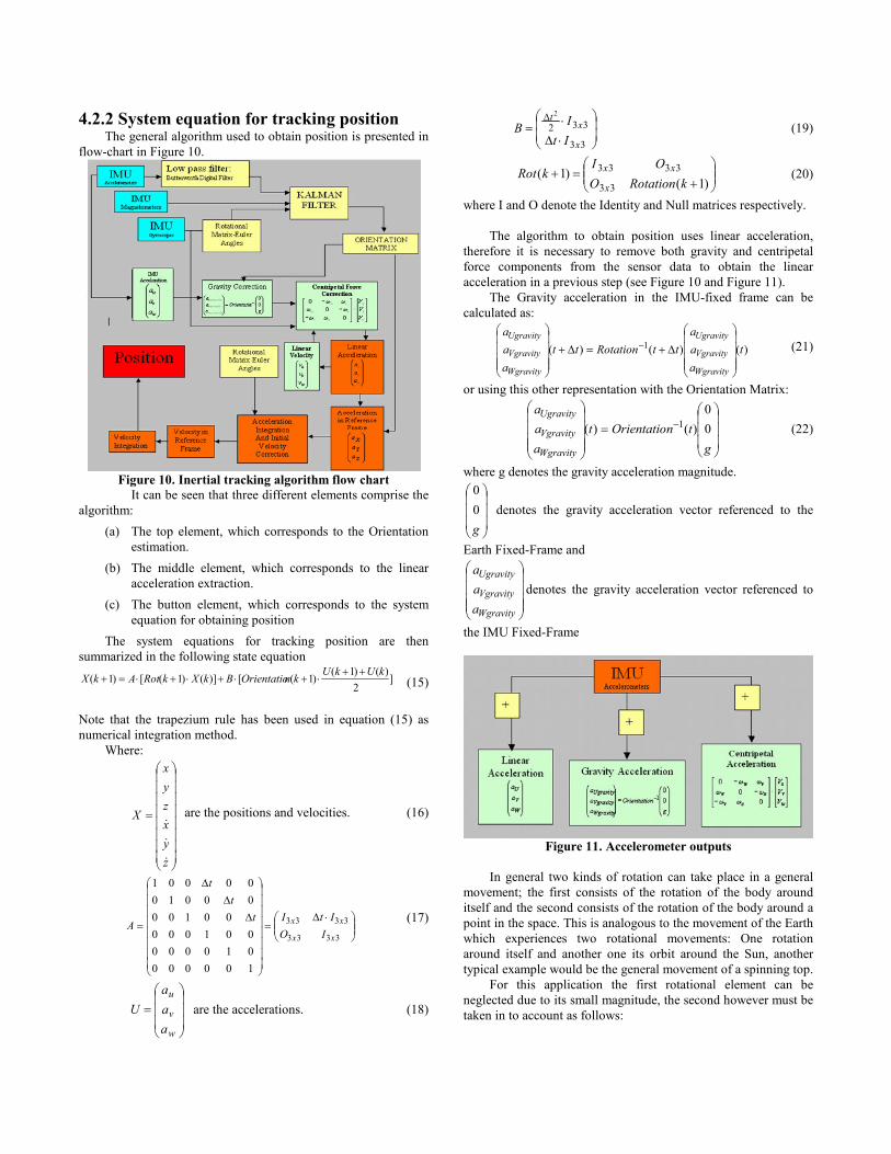
4.2.2 System equation for tracking position The general algorithm used to obtain position is presented in
flow-chart in Figure 10.
Figure 10. Inertial tracking algorithm flow chart
It can be seen that three different elements comprise the
algorithm:
(a) The top element, which corresponds to the Orientation
estimation.
(b) The middle element, which corresponds to the linear
acceleration extraction.
(c) The button element, which corresponds to the system
equation for obtaining position
The system equations for tracking position are then
summarized in the following state equation
]2
)()1()1([)]()1([)1(
kUkUknOrientatioBkXkRotAkX
++⋅+⋅+⋅+⋅=+ (15)
Note that the trapezium rule has been used in equation (15) as
numerical integration method.
Where:
=
z
y
x
z
y
x
X
&
&
&
are the positions and velocities. (16)
⋅∆=
∆
∆
∆
=3333
3333
100000
010000
001000
00100
00010
00001
xx
xx
IO
ItIt
t
t
A (17)
=
w
v
u
a
a
a
U are the accelerations. (18)
⋅∆
⋅=∆
33
332
2
x
xt
It
IB (19)
+=+
)1()1(
33
3333
kRotationO
OIkRot
x
xx (20)
where I and O denote the Identity and Null matrices respectively.
The algorithm to obtain position uses linear acceleration,
therefore it is necessary to remove both gravity and centripetal
force components from the sensor data to obtain the linear
acceleration in a previous step (see Figure 10 and Figure 11).
The Gravity acceleration in the IMU-fixed frame can be
calculated as:
)()()( 1 t
a
a
a
ttRotationtt
a
a
a
Wgravity
Vgravity
Ugravity
Wgravity
Vgravity
Ugravity
∆+=∆+
− (21)
or using this other representation with the Orientation Matrix:
=
−
g
tnOrientatiot
a
a
a
Wgravity
Vgravity
Ugravity
0
0
)()( 1 (22)
where g denotes the gravity acceleration magnitude.
g
0
0
denotes the gravity acceleration vector referenced to the
Earth Fixed-Frame and
Wgravity
Vgravity
Ugravity
a
a
a
denotes the gravity acceleration vector referenced to
the IMU Fixed-Frame
Figure 11. Accelerometer outputs
In general two kinds of rotation can take place in a general
movement; the first consists of the rotation of the body around
itself and the second consists of the rotation of the body around a
point in the space. This is analogous to the movement of the Earth
which experiences two rotational movements: One rotation
around itself and another one its orbit around the Sun, another
typical example would be the general movement of a spinning top.
For this application the first rotational element can be
neglected due to its small magnitude, the second however must be
taken in to account as follows:
⋅
−
−
−
=
W
V
U
uv
uw
vw
alwcentripet
alvcentripet
alucentripet
V
V
V
a
a
a
0
0
0
ωωωω
ωω (23)
The centripetal force is given as the cross product of the
angular velocity and the linear velocity. This velocity is the linear
velocity on the IMU axes obtained in the IMU Fixed-frame,
according to the nomenclature followed; this is the velocity in the
axes U, V, W.
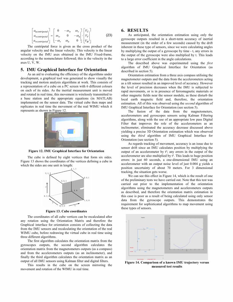
5. IMU Graphical Interface for Orientation As an aid to evaluating the efficiency of the algorithms under
development, a graphical tool was generated to show visually the
tracking and motion analysis algorithms at work. This consists of
a representation of a cube on a PC screen with 6 different colours
on each of its sides. As the inertial measurement unit is moved
and rotated in real time, this movement is wirelessly transmitted to
a base station and the appropriate equations (in MATLAB)
implemented on the sensor data. The virtual cube then maps and
replicates in real time the movement of the real WIMU which it
represents as shown in Figure 12.
Figure 12. IMU Graphical Interface for Orientation
The cube is defined by eight vertices that form six sides.
Figure 13 shows the coordinates of the vertices defining a cube in
which the sides are one unit in length:
Figure 13. Cube coordinates
The coordinates of all cube vertices can be recalculated after
any rotation using the Orientation Matrix and therefore the
Graphical interface for orientation consists of collecting the data
from the IMU sensors and recalculating the orientation of the real
WIMU cube, before redrawing the virtual cube in real time using
three different algorithms.
The first algorithm calculates the orientation matrix from the
gyroscopes outputs, the second algorithm calculates the
orientation matrix from the magnetometers outputs (as a compass)
and from the accelerometers outputs (as an inclinometer), and
finally the third algorithm calculates the orientation matrix as an
output of all IMU sensors using Kalman filter and digital filters.
This results in the cube on the screen mirroring the
movement and rotation of the WIMU in real time.
6. RESULTS As anticipated, the orientation estimation using only the
gyroscope outputs resulted in a short-term accuracy of inertial
measurement (in the order of a few seconds) caused by the drift
inherent in these type of sensors, since we were calculating angles
by multiplying the output of a gyroscope by time - t, any errors in
the output of the gyroscope were also multiplied by t. This leads
to a large error coefficient in the angle calculations.
The described above was experimented using the first
algorithm of IMU Graphical Interface for Orientation (as
described in section 5).
Orientation estimation from a three axis compass utilising the
magnetometer outputs and the data from the accelerometers acting
as a tilt sensor resulted in an improved level of accuracy. However
the level of precision decreases when the IMU is subjected to
rapid movements, or is in presence of ferromagnetic materials or
other magnetic fields near the sensor module, as these disturb the
local earth magnetic field and, therefore, the orientation
estimation. All of this was observed using the second algorithm of
IMU Graphical Interface for Orientation (see section 5).
The fusion of the data from the magnetometers,
accelerometers and gyroscopes sensors using Kalman Filtering
algorithms, along with the use of an appropriate low pass Digital
Filter that improves the role of the accelerometers as an
inclinometer, eliminated the accuracy decrease discussed above
yielding a precise 3D Orientation estimation which was observed
using the third algorithm of IMU Graphical Interface for
Orientation (see section 5).
As regards tracking of movement, accuracy is an issue due to
sensor drift since an IMU calculates position by multiplying the
output of an accelerometer by t²; any errors in the output of the
accelerometer are also multiplied by t². This leads to huge position
errors: in just 60 seconds, a one-dimensional IMU using an
accelerometer with an output noise level of just 0.004 g yields a
position uncertainty of about 70 meters. For 3 dimensional
tracking, the situation gets worse.
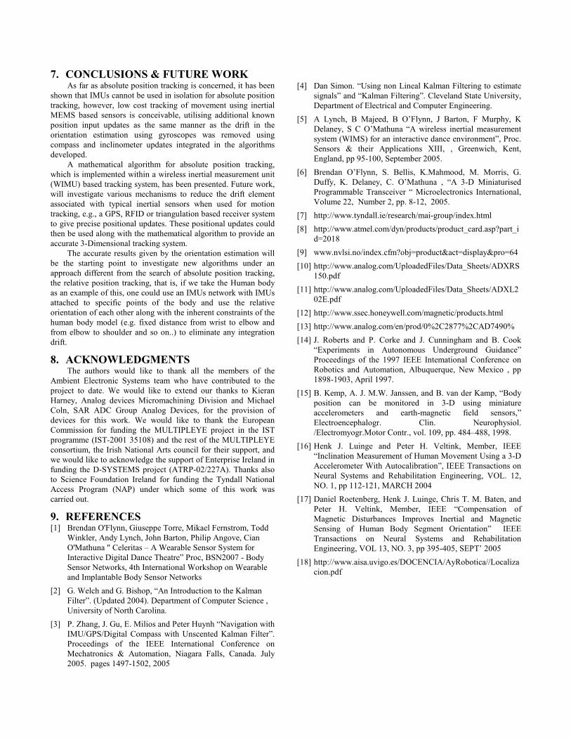
We can see this effect in Figure 14, which is the result of one
of the preliminary tests we have carried out. Note that this test was
carried out prior to the implementation of the orientation
algorithms using the magnetometers and accelerometers outputs
as described, and therefore the orientation matrix estimation in
this case is poor as a result of being calculated using only sensor
data from the gyroscope outputs. This demonstrates the
requirement for sophisticated algorithms to map movement using
these types of sensors.
Figure 14. Comparison of a known IMU trajectory versus
measured test results
7. CONCLUSIONS & FUTURE WORK As far as absolute position tracking is concerned, it has been
shown that IMUs cannot be used in isolation for absolute position
tracking, however, low cost tracking of movement using inertial
MEMS based sensors is conceivable, utilising additional known
position input updates as the same manner as the drift in the
orientation estimation using gyroscopes was removed using
compass and inclinometer updates integrated in the algorithms
developed.
A mathematical algorithm for absolute position tracking,
which is implemented within a wireless inertial measurement unit
(WIMU) based tracking system, has been presented. Future work,
will investigate various mechanisms to reduce the drift element
associated with typical inertial sensors when used for motion
tracking, e.g., a GPS, RFID or triangulation based receiver system
to give precise positional updates. These positional updates could
then be used along with the mathematical algorithm to provide an
accurate 3-Dimensional tracking system.
The accurate results given by the orientation estimation will
be the starting point to investigate new algorithms under an
approach different from the search of absolute position tracking,
the relative position tracking, that is, if we take the Human body
as an example of this, one could use an IMUs network with IMUs
attached to specific points of the body and use the relative
orientation of each other along with the inherent constraints of the
human body model (e.g. fixed distance from wrist to elbow and
from elbow to shoulder and so on..) to eliminate any integration
drift.
8. ACKNOWLEDGMENTS The authors would like to thank all the members of the
Ambient Electronic Systems team who have contributed to the
project to date. We would like to extend our thanks to Kieran
Harney, Analog devices Micromachining Division and Michael
Coln, SAR ADC Group Analog Devices, for the provision of
devices for this work. We would like to thank the European
Commission for funding the MULTIPLEYE project in the IST
programme (IST-2001 35108) and the rest of the MULTIPLEYE
consortium, the Irish National Arts council for their support, and
we would like to acknowledge the support of Enterprise Ireland in
funding the D-SYSTEMS project (ATRP-02/227A). Thanks also
to Science Foundation Ireland for funding the Tyndall National
Access Program (NAP) under which some of this work was
carried out.
9. REFERENCES [1] Brendan O'Flynn, Giuseppe Torre, Mikael Fernstrom, Todd
Winkler, Andy Lynch, John Barton, Philip Angove, Cian
O'Mathuna " Celeritas – A Wearable Sensor System for
Interactive Digital Dance Theatre” Proc, BSN2007 - Body
Sensor Networks, 4th International Workshop on Wearable
and Implantable Body Sensor Networks
[2] G. Welch and G. Bishop, “An Introduction to the Kalman
Filter”. (Updated 2004). Department of Computer Science ,
University of North Carolina.
[3] P. Zhang, J. Gu, E. Milios and Peter Huynh “Navigation with IMU/GPS/Digital Compass with Unscented Kalman Filter”.
Proceedings of the IEEE International Conference on
Mechatronics & Automation, Niagara Falls, Canada. July
2005. pages 1497-1502, 2005
[4] Dan Simon. “Using non Lineal Kalman Filtering to estimate signals” and “Kalman Filtering”. Cleveland State University,
Department of Electrical and Computer Engineering.
[5] A Lynch, B Majeed, B O’Flynn, J Barton, F Murphy, K Delaney, S C O’Mathuna “A wireless inertial measurement
system (WIMS) for an interactive dance environment”, Proc.
Sensors & their Applications XIII, , Greenwich, Kent,
England, pp 95-100, September 2005.
[6] Brendan O’Flynn, S. Bellis, K.Mahmood, M. Morris, G. Duffy, K. Delaney, C. O’Mathuna , “A 3-D Miniaturised
Programmable Transceiver “ Microelectronics International,
Volume 22, Number 2, pp. 8-12, 2005.
[7] http://www.tyndall.ie/research/mai-group/index.html
[8] http://www.atmel.com/dyn/products/product_card.asp?part_id=2018
[9] www.nvlsi.no/index.cfm?obj=product&act=display&pro=64
[10] http://www.analog.com/UploadedFiles/Data_Sheets/ADXRS150.pdf
[11] http://www.analog.com/UploadedFiles/Data_Sheets/ADXL202E.pdf
[12] http://www.ssec.honeywell.com/magnetic/products.html
[13] http://www.analog.com/en/prod/0%2C2877%2CAD7490%
[14] J. Roberts and P. Corke and J. Cunningham and B. Cook “Experiments in Autonomous Underground Guidance”
Proceedings of the 1997 IEEE Intemational Conference on
Robotics and Automation, Albuquerque, New Mexico , pp
1898-1903, April 1997.
[15] B. Kemp, A. J. M.W. Janssen, and B. van der Kamp, “Body
position can be monitored in 3-D using miniature
accelerometers and earth-magnetic field sensors,”
Electroencephalogr. Clin. Neurophysiol.
/Electromyogr.Motor Contr., vol. 109, pp. 484–488, 1998.
[16] Henk J. Luinge and Peter H. Veltink, Member, IEEE “Inclination Measurement of Human Movement Using a 3-D
Accelerometer With Autocalibration”, IEEE Transactions on
Neural Systems and Rehabilitation Engineering, VOL. 12,
NO. 1, pp 112-121, MARCH 2004
[17] Daniel Roetenberg, Henk J. Luinge, Chris T. M. Baten, and Peter H. Veltink, Member, IEEE “Compensation of
Magnetic Disturbances Improves Inertial and Magnetic
Sensing of Human Body Segment Orientation” IEEE
Transactions on Neural Systems and Rehabilitation
Engineering, VOL 13, NO. 3, pp 395-405, SEPT’ 2005
[18] http://www.aisa.uvigo.es/DOCENCIA/AyRobotica//Localizacion.pdf
Recommended