NPTEL – Physics – Physics of Magnetic recording
Joint initiative of IITs and IISc – Funded by MHRD Page 1 of 20
Module 1: Introduction
Lecture 01: History and overview of magnetic recording
Objectives:
This module will serve as a necessary introduction to the course as well as the
manifestation of the magnetic anisotropy property of solid state materials focused to
magnetic recording devices, viz., magnetism. We will start our quest with a look at the
historical development of magnetic recording techniques. This would not only provide an
account of the evolution of the magnetic recording techniques, but would also point
towards the future of recording process. This would be followed by understanding the
directional dependence of magnetic properties of magnetic materials or magnetic
anisotropy and the factors that influence this. We will close this chapter by taking a look
at the soft and hard magnetic materials and their characteristics.
Therefore, the following five lectures would cover the following topics:
1. How magnetic recording has evolved over the years?
2. What are the different forms of magnetic media?
3. What is magnetic anisotropy energy and what are the factors that contribute to it?
4. What is magnetostriction?
5. What are soft and hard magnetic materials?
Figure 1.1: Schematic drawing of analogue magnetic recording.
NPTEL – Physics – Physics of Magnetic recording
Joint initiative of IITs and IISc – Funded by MHRD Page 2 of 20
Introduction:
Magnetic recording referring to the storage of data on a magnetized medium is generally
classified into two groups of related technologies: media and recording heads. While the
first one consists of all technologies concerned with the production and the use of
magnetic disks and tapes for storing information, the later one covers all the technologies
connected to the process of writing information on the media or reading information from
the written media.
Digital recording for storage of computer was first developed by IBM. Magnetic disk
drive, called RAMAC, was available in 1957. Earlier to this, magnetic tapes was invented
using a paper tape coated either with dried ferromagnetic liquid or with iron powder.
Later oxide tapes were developed by 3M Corporation, which ensured the availability of
audio recorders in 1940 and video recorders in 1956.On the other hand, the analogue
magnetic recording was first demonstrated by a Danish engineer Poulsen by recording
acoustical signals on a ferromagnetic wire using an electromagnet connected to a
microphone, as shown in Figure 1.1. However, there were two major problems in the
recording process: (i) the reproduction of signal was very weak due to the absence of an
amplifier, and (ii) low signal to noise ratio due to the nonlinear nature of the recording
process.
NPTEL – Physics – Physics of Magnetic recording
Joint initiative of IITs and IISc – Funded by MHRD Page 3 of 20
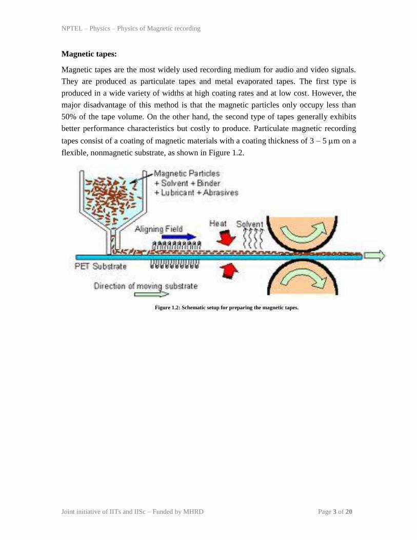
Magnetic tapes:
Magnetic tapes are the most widely used recording medium for audio and video signals.
They are produced as particulate tapes and metal evaporated tapes. The first type is
produced in a wide variety of widths at high coating rates and at low cost. However, the
major disadvantage of this method is that the magnetic particles only occupy less than
50% of the tape volume. On the other hand, the second type of tapes generally exhibits
better performance characteristics but costly to produce. Particulate magnetic recording
tapes consist of a coating of magnetic materials with a coating thickness of 3 – 5 m on a
flexible, nonmagnetic substrate, as shown in Figure 1.2.
Figure 1.2: Schematic setup for preparing the magnetic tapes.
NPTEL – Physics – Physics of Magnetic recording
Joint initiative of IITs and IISc – Funded by MHRD Page 4 of 20
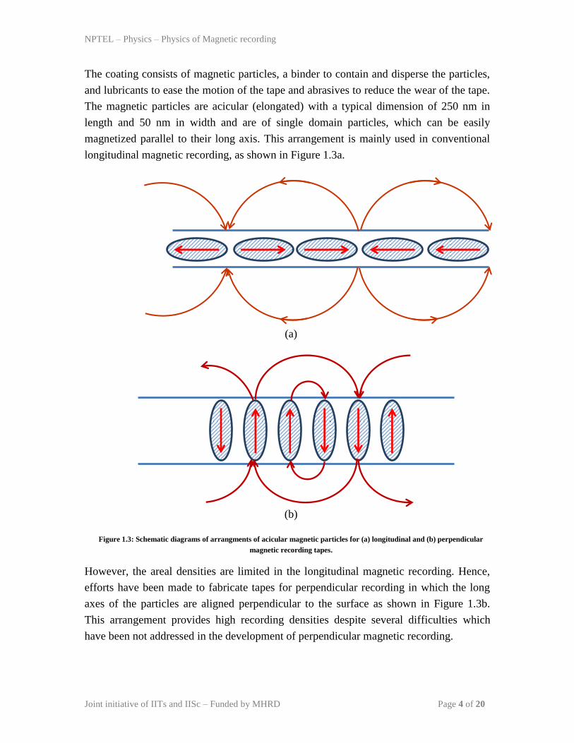
The coating consists of magnetic particles, a binder to contain and disperse the particles,
and lubricants to ease the motion of the tape and abrasives to reduce the wear of the tape.
The magnetic particles are acicular (elongated) with a typical dimension of 250 nm in
length and 50 nm in width and are of single domain particles, which can be easily
magnetized parallel to their long axis. This arrangement is mainly used in conventional
longitudinal magnetic recording, as shown in Figure 1.3a.
(a)
(b)
Figure 1.3: Schematic diagrams of arrangments of acicular magnetic particles for (a) longitudinal and (b) perpendicular
magnetic recording tapes.
However, the areal densities are limited in the longitudinal magnetic recording. Hence,
efforts have been made to fabricate tapes for perpendicular recording in which the long
axes of the particles are aligned perpendicular to the surface as shown in Figure 1.3b.
This arrangement provides high recording densities despite several difficulties which
have been not addressed in the development of perpendicular magnetic recording.
NPTEL – Physics – Physics of Magnetic recording
Joint initiative of IITs and IISc – Funded by MHRD Page 5 of 20
Module 1: Introduction
Lecture 02: History and overview of magnetic recording
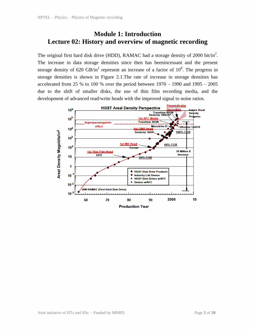
The original first hard disk drive (HDD), RAMAC had a storage density of 2000 bit/in2.
The increase in data storage densities since then has beenincessant and the present
storage density of 620 GB/in2 represent an increase of a factor of 10
8. The progress in
storage densities is shown in Figure 2.1.The rate of increase in storage densities has
accelerated from 25 % to 100 % over the period between 1970 – 1990 and 1995 – 2005
due to the shift of smaller disks, the use of thin film recording media, and the
development of advanced read/write heads with the improved signal to noise ratios.
NPTEL – Physics – Physics of Magnetic recording
Joint initiative of IITs and IISc – Funded by MHRD Page 6 of 20
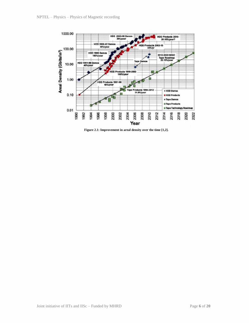
Figure 2.1: Improvement in areal density over the time [1,2].
NPTEL – Physics – Physics of Magnetic recording
Joint initiative of IITs and IISc – Funded by MHRD Page 7 of 20
(a)
(b)
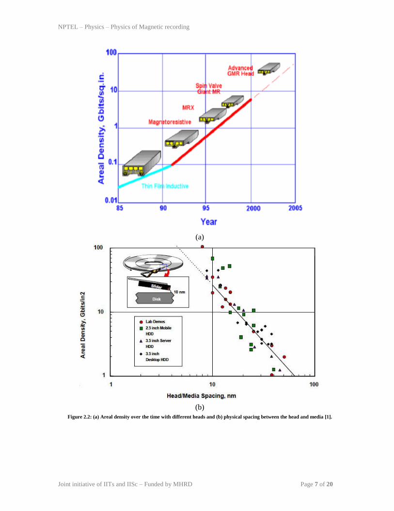
Figure 2.2: (a) Areal density over the time with different heads and (b) physical spacing between the head and media [1].

NPTEL – Physics – Physics of Magnetic recording
Joint initiative of IITs and IISc – Funded by MHRD Page 8 of 20
The projections for the current and future HDD from Western Digital Corporation over
the time is also shown in Figure 2.1, in which it is imagined that the development of
smaller magnetoresistive (MR) read heads, improvement in actuation between the MR
head and media surface, as shown in Figure 2.2, and micromechanics will provide the
next stages of evolution. It is also proposed to follow bit patterned media, and scanning
tunnelling microscope (STM) like storage in the future.
Materials suitable for magnetic recording:
The most widely used magnetic recording materials in the earlier days is gamma ferric
oxide (-Fe2O3) which has been used in magnetic tapes since 1937. The coercivities of
such tapes were in the range of 250 – 400 Oe for the particles of size aspect ratio of 10:1
on length to diameter ratio[3]. The magnetic properties of these particles were not
affected by the working environment in the vicinity of the room temperatures as the Curie
temperature of the particles was more than 500 oC. The magnetic properties of the Fe2O3
particles were further improved by modifying the surface using Co. The coercivity of the
Co surface modified Fe2O3 increased to about 900 Oe [3] due to the increase in
anisotropy of the materials with the Co addition. Later, the chromium dioxide powder
was exercised for recording due to their high saturation magnetization as compared to the
iron oxide. However, it is more expensive than the iron oxide which reduced its
commercial attraction. Iron powder was also used as a recording medium. This has
considerably high saturation magnetization (1700 emu/cc) than the oxide particulate
media and had a high coercivity of 1.4 kOe. Eventually, the thin metallic alloy films were
proposed as a magnetic medium for high performance, high storage density, hard disk
drives. Hexagonal ferrites with high coercivity of 4.6 kOe for the disk shaped barium
ferrite particles have also been proposed as one of the suitable materials for magnetic
recording. CoCrPt based alloys were the recent outcome for recording as they have
improved corrosion resistance compared to pure cobalt. In last few decades, serious
efforts have been made to develop metallic thin film recording medium using various
types of technology, including the perpendicular magnetic recording media in which the
magnetic domains are oriented with the magnetizations normal to the plan of the medium
have been pioneered by Iwasaki in Japan [4].More details regarding the properties of the
materials used for recording is provided in later lectures.
NPTEL – Physics – Physics of Magnetic recording
Joint initiative of IITs and IISc – Funded by MHRD Page 9 of 20
Another area of interest in magnetic recording is that of magneto-optical devices [5].
These make use of the Faraday and Kerr effects in which the direction of polarization of
light is rotated in the presence of a magnetic field. The advantage of the magneto-optical
disks is to develop recording disk with significantly increased densities with faster access
time. However, the concept of magneto-optical recording has currently not been
continued, as the recording of information depends on thermomagnetic magnetization of
the materials.
References:
[1]. http://www.hitachigst.com
[2]. http://www.wdc.com
[3]. R.E. Hummel, Electronic Properties of materials, Springer, 2012, Chapter 17.
[4]. S. Iwasaki, IEEE Trans. Magn. 16 (1980) 71.
[5]. R.J. Gambino, T. Suzuki, Magneto-optical recording materials, Wiley-IEEE Press,
1999.
NPTEL – Physics – Physics of Magnetic recording
Joint initiative of IITs and IISc – Funded by MHRD Page 10 of 20
Module 1: Introduction
Lecture 03: Magnetic Anisotropy
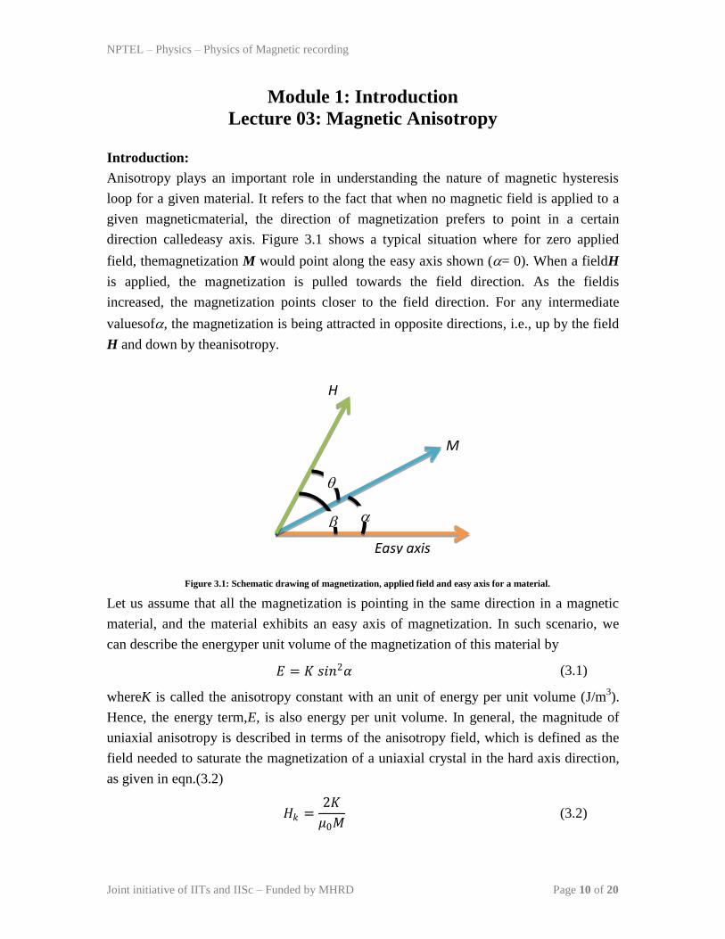
Introduction:
Anisotropy plays an important role in understanding the nature of magnetic hysteresis
loop for a given material. It refers to the fact that when no magnetic field is applied to a
given magneticmaterial, the direction of magnetization prefers to point in a certain
direction calledeasy axis. Figure 3.1 shows a typical situation where for zero applied
field, themagnetization M would point along the easy axis shown (= 0). When a fieldH
is applied, the magnetization is pulled towards the field direction. As the fieldis
increased, the magnetization points closer to the field direction. For any intermediate
valuesof, the magnetization is being attracted in opposite directions, i.e., up by the field
H and down by theanisotropy.
Figure 3.1: Schematic drawing of magnetization, applied field and easy axis for a material.
Let us assume that all the magnetization is pointing in the same direction in a magnetic
material, and the material exhibits an easy axis of magnetization. In such scenario, we
can describe the energyper unit volume of the magnetization of this material by
𝐸 = 𝐾 𝑠𝑖𝑛2𝛼 (3.1)
whereK is called the anisotropy constant with an unit of energy per unit volume (J/m3).
Hence, the energy term,E, is also energy per unit volume. In general, the magnitude of
uniaxial anisotropy is described in terms of the anisotropy field, which is defined as the
field needed to saturate the magnetization of a uniaxial crystal in the hard axis direction,
as given in eqn.(3.2)
𝐻𝑘 =2𝐾
𝜇0𝑀 (3.2)
H
M
Easy axis

NPTEL – Physics – Physics of Magnetic recording
Joint initiative of IITs and IISc – Funded by MHRD Page 11 of 20
In general, the energy of the magnetization is given by,
𝐸 = 𝐾 𝑠𝑖𝑛2𝛼 − 𝜇0𝑀𝐻 𝑐𝑜𝑠 𝛽 − 𝛼 (3.3)
where, the first term is anisotropy energy. The second term is due to the magnetic field
and the difference in the angle (-) is the angle between H and M. In order to get
equilibrium, we required firstderivative to be zero. Therefore, taking derivative of
eqn.(3.3) with respect to the angle results,
𝑑𝐸
𝑑𝛼= 2𝐾 sin 𝛼 cos 𝛼 − 𝜇0𝑀𝐻 𝑠𝑖𝑛 𝛽 − 𝛼 = 0 (3.4)
Taking the value of as 90o for the equilibrium angle for the magnetization relative to
the easy axis and considering the eqn.(3.2) gives
sin 𝛼 =𝐻
𝐻𝑘 (3.5)
The above eqn. indicates that when H = 0, the magnetization points along the easy axis
and when H = Hk, the magnetization points along the direction of H.For any intermediate
value of the applied field, the magnetization points at a value of angle given by eqn.(3.5)
rotating smoothly between the easy axis and the applied field.
Figure 3.2: Magnetization of single crystals of Iron, Nickel and Cobalt.
NPTEL – Physics – Physics of Magnetic recording
Joint initiative of IITs and IISc – Funded by MHRD Page 12 of 20
Magnetocrystalline anisotropy:
Figure 3.2 depicts the initial magnetization curves of single crystals of the different 3d
ferromagnetic elements. It is clearly seen that they show a different approach to
saturation when magnetized in different directions. For example, the iron shows a 100
as easy directions and 111 as hard directions, while the nickel exhibits 111 as easy
axis and 100 as hard directions. This property can be understood by analysing the
development of anisotropy energy in different symmetries as given below:
For Hexagonal:
𝐸𝑎 = 𝐾1 sin2 𝜃 + 𝐾2 sin4 𝜃 + 𝐾3 sin6 𝜃 + 𝐾3′ sin6 𝜃 sin 6𝜙
For Tetragonal:
𝐸𝑎 = 𝐾1 sin2 𝜃 + 𝐾2 sin4 𝜃 + 𝐾2′ sin4 𝜃 cos 4𝜙 + 𝐾3 sin6 𝜃
+ 𝐾3′ sin6 𝜃 sin 6𝜙
For Cubic:
𝐸𝑎 = 𝐾1𝑐 𝛼12𝛼2
2 + 𝛼22𝛼3
2 + 𝛼32𝛼1
2 + 𝐾2𝑐 𝛼12𝛼2
2𝛼32
(3.6)
wherei are the direction cosines of the magnetization. The K1c term is equivalent to
𝐾1𝑐 = 𝐾1𝑐 sin2 𝜃 𝑐𝑜𝑠2 𝜙 sin2 𝜙 + cos2 𝜃 sin2 𝜃 . When, =0, =0, this term reduces to
eqn.(3.1).
Origin of magnetocrystalline anisotropy:
There are two distinct sources of magnetocrystalline anisotropy: (i) single-ion
contributions and (ii) two-ion contributions. The first one is essentially due to the
electrostatic interaction of the orbitals containing the magnetic electrons with the
potential created at the atomic site by the rest of the crystal. This crystal field interaction
stabilizes a particular orbital and by spin-orbit interaction, the magnetic moment is
aligned in a particular crystallographic direction. For example, a uniaxial crystal having
21028
ions/m3, described by a spin Hamiltonian DS
2 with D/kB = 1 K and S = 2 will have
anisotropy constant K1 = nDS2 = 1.110
6 J/m
3.
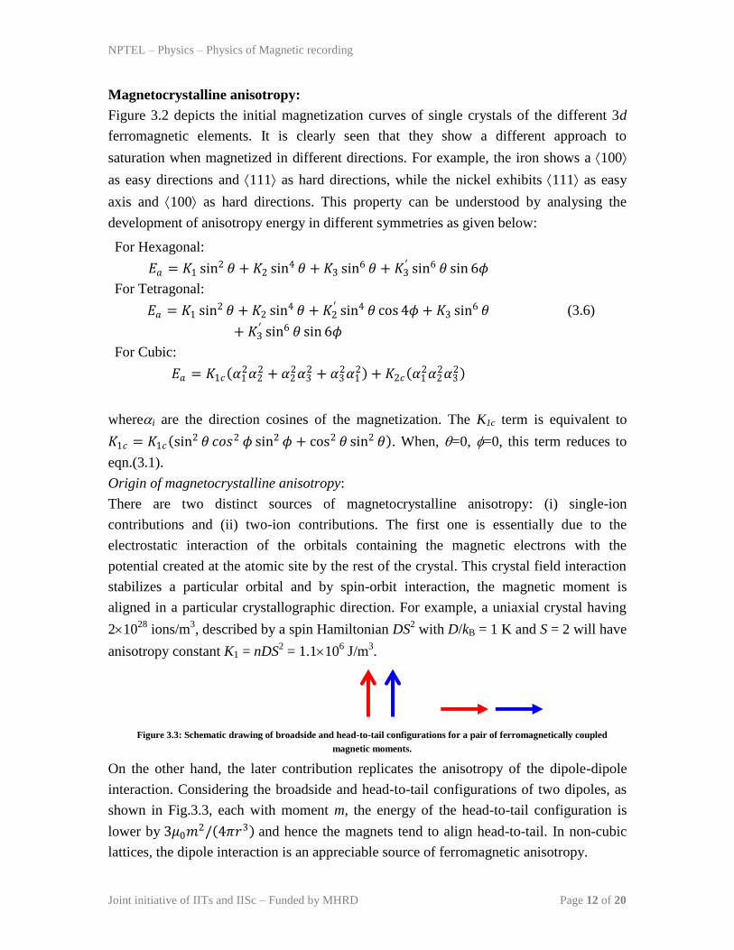
Figure 3.3: Schematic drawing of broadside and head-to-tail configurations for a pair of ferromagnetically coupled
magnetic moments.
On the other hand, the later contribution replicates the anisotropy of the dipole-dipole
interaction. Considering the broadside and head-to-tail configurations of two dipoles, as
shown in Fig.3.3, each with moment m, the energy of the head-to-tail configuration is
lower by 3𝜇0𝑚2/ 4𝜋𝑟3 and hence the magnets tend to align head-to-tail. In non-cubic
lattices, the dipole interaction is an appreciable source of ferromagnetic anisotropy.
NPTEL – Physics – Physics of Magnetic recording
Joint initiative of IITs and IISc – Funded by MHRD Page 13 of 20
Module 1: Introduction
Lecture 04: Magnetic Anisotropy
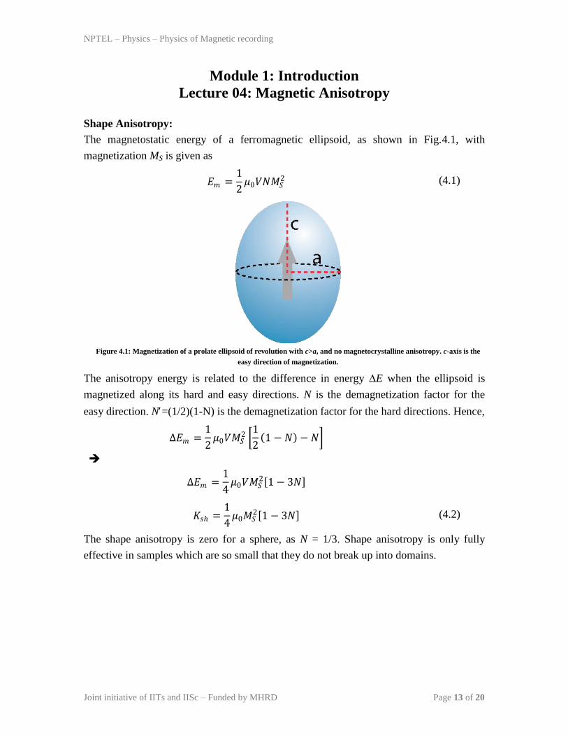
Shape Anisotropy:
The magnetostatic energy of a ferromagnetic ellipsoid, as shown in Fig.4.1, with
magnetization MS is given as
𝐸𝑚 =1
2𝜇0𝑉𝑁𝑀𝑆
2 (4.1)
Figure 4.1: Magnetization of a prolate ellipsoid of revolution with c>a, and no magnetocrystalline anisotropy. c-axis is the
easy direction of magnetization.
The anisotropy energy is related to the difference in energy E when the ellipsoid is
magnetized along its hard and easy directions. N is the demagnetization factor for the
easy direction. N=(1/2)(1-N) is the demagnetization factor for the hard directions. Hence,
∆𝐸𝑚 =1
2𝜇0𝑉𝑀𝑆
2 1
2 1 − 𝑁 − 𝑁
∆𝐸𝑚 =1
4𝜇0𝑉𝑀𝑆
2 1 − 3𝑁
𝐾𝑠ℎ =1
4𝜇0𝑀𝑆
2 1 − 3𝑁 (4.2)
The shape anisotropy is zero for a sphere, as N = 1/3. Shape anisotropy is only fully
effective in samples which are so small that they do not break up into domains.

NPTEL – Physics – Physics of Magnetic recording
Joint initiative of IITs and IISc – Funded by MHRD Page 14 of 20
Induced Anisotropy:
In some materials, the magneticanisotropy can be induced by many ways: (i) fabricate a
film in the presence of a magnetic field, (ii) heat treat the materials in the presence of
external applied magnetic field, and (iii) apply uniaxial stress.In the first two cases, after
such treatment, the material may exhibit an easyaxis of magnetization that points in the
direction of the magnetic field that was applied.This induced anisotropy is certainly
independent of any crystalline anisotropy or anyother form of anisotropy that might be
present. Figure 4.2 shows the typical example of inducing the anisotropy in the
ferromagnetic materials by field annealing. One of the classical materials that exhibits the
magnetic field induced anisotropy is Permalloy. If there are no stray magnetic fields
present during deposition, then the easy axis of anisotropy will be found to be in the
direction of theearth's magnetic field.
Figure 4.2: Magnetization of a thin film with induced anisotropy created by annealing in a magnetic field. The sheared
(open) loop in a (b) is observed when the measuring field H is applied perpendicular (parallel) to the annealing field
direction.
NPTEL – Physics – Physics of Magnetic recording
Joint initiative of IITs and IISc – Funded by MHRD Page 15 of 20
In the last case, the uniaxial anisotropy is induced by applying uniaxial stress in a
ferromagnetic solid. The magnitude of the stress-induced anisotropy is
𝐾𝑢𝜎 =3
2𝜎𝜆𝑆 (4.3)
where S is the saturation magnetostriction. Both the single-ion and two-ion anisotropy
contribute to the stress induced anisotropy. The largest values of uniaxial anisotropy are
found in hexagonal and other uniaxial crystals. Smallest values are found in cubic alloys
and amorphous ferromagnets.
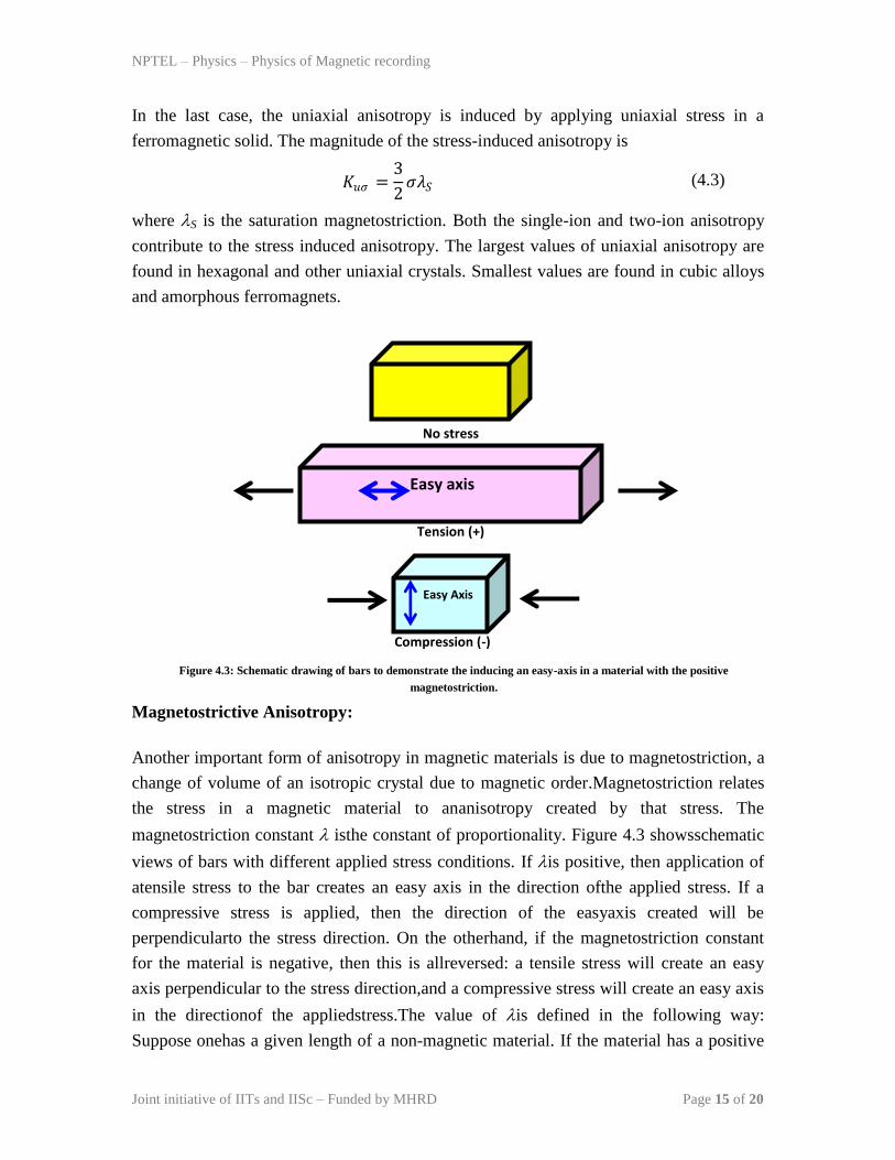
Figure 4.3: Schematic drawing of bars to demonstrate the inducing an easy-axis in a material with the positive
magnetostriction.
Magnetostrictive Anisotropy:
Another important form of anisotropy in magnetic materials is due to magnetostriction, a
change of volume of an isotropic crystal due to magnetic order.Magnetostriction relates
the stress in a magnetic material to ananisotropy created by that stress. The
magnetostriction constant isthe constant of proportionality. Figure 4.3 showsschematic
views of bars with different applied stress conditions. If is positive, then application of
atensile stress to the bar creates an easy axis in the direction ofthe applied stress. If a
compressive stress is applied, then the direction of the easyaxis created will be
perpendicularto the stress direction. On the otherhand, if the magnetostriction constant
for the material is negative, then this is allreversed: a tensile stress will create an easy
axis perpendicular to the stress direction,and a compressive stress will create an easy axis
in the directionof the appliedstress.The value of is defined in the following way:
Suppose onehas a given length of a non-magnetic material. If the material has a positive
No stress
Easy Axis
Compression (-)
Easy axis
Tension (+)

NPTEL – Physics – Physics of Magnetic recording
Joint initiative of IITs and IISc – Funded by MHRD Page 16 of 20
value of, then causingthe materialtobecomemagneticwill cause the materialto lengthenor
stretch in the direction of the magnetization. The fractional increase in length isdefined as
the magnetostriction constant, . If the material has a negative value of, then the
material will shorten in the direction of the magnetization.
Quiz:
(1) What is anisotropy?
(2) What is the role of anisotropy in the magnetic materials?
(3) Which materials possess high magnetocrystalline anisotropy? Why?
(4) Summarize the different ways to induce the anisotropy in the magnetic materials.
(5) Which type of materials exhibit large shape anisotropy? Can the shape anisotropy
play a crucial role in bulk materials?
(6) Is it possible to produce a permanent magnet of arbitrary shapeusing shape anisotropy
alone?
NPTEL – Physics – Physics of Magnetic recording
Joint initiative of IITs and IISc – Funded by MHRD Page 17 of 20
Module 1: Introduction
Lecture 05: Soft and Hard magnetic materials and Stoner-
Wohlfarth theory
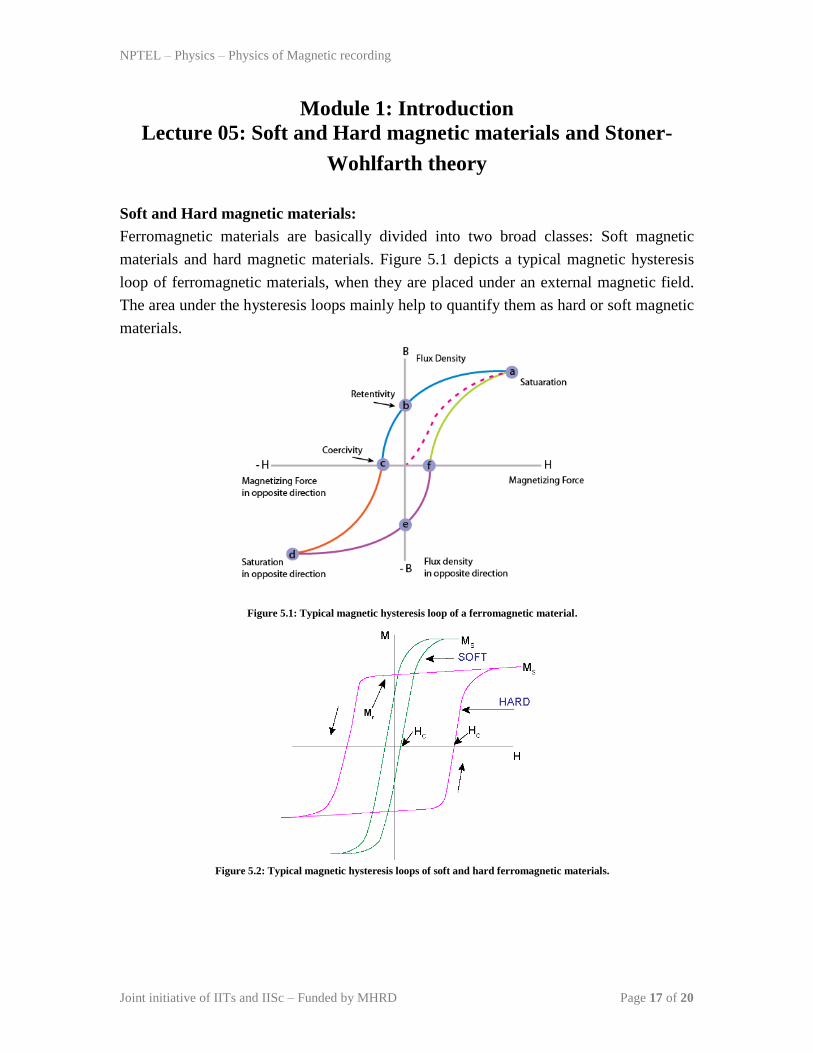
Soft and Hard magnetic materials:
Ferromagnetic materials are basically divided into two broad classes: Soft magnetic
materials and hard magnetic materials. Figure 5.1 depicts a typical magnetic hysteresis
loop of ferromagnetic materials, when they are placed under an external magnetic field.
The area under the hysteresis loops mainly help to quantify them as hard or soft magnetic
materials.
Figure 5.1: Typical magnetic hysteresis loop of a ferromagnetic material.
Figure 5.2: Typical magnetic hysteresis loops of soft and hard ferromagnetic materials.

NPTEL – Physics – Physics of Magnetic recording
Joint initiative of IITs and IISc – Funded by MHRD Page 18 of 20
Figure 5.2 displays comparative magnetic hysteresis loops for both soft and hard
magnetic materials. Hard magnetic materials generally show low initial permeability
(close to the origin in Fig.5.1) and high coercive force (HC>1000 Oe). These materials are
generally used for disk media or for a permanent magnet application. On the other hand,
soft magnetic materials exhibit high initial permeability and also low coercivity (<100
Oe). These materials are used for a transformer or a magnetic head application. Since
both the types of ferromagnetic materials have different magnetic parameters associated
with the hysteresis, their magnetization reversal behaviour would also be different. Now,
we shall try to understand the magnetization reversal behaviour using Stoner-
Wohlfarth(SW) model.
Figure 5.3: Schematic of SW particle.
Figure 5.4: Variation of magnetic hysteresis loop of a SW particle with angle,, between the field direction and easy axis.
H
M
Easy axis
NPTEL – Physics – Physics of Magnetic recording
Joint initiative of IITs and IISc – Funded by MHRD Page 19 of 20
Stoner-Wohlfarth Model:
This is a simple analytical model describing the hysteresis. Consider a uniformly
magnetized ellipsoid with uniaxial anisotropy of shape or magnetocrystalline origin
(called as SW particle, as shown in Fig.5.3) in a field applied at an angle to the
anisotropy axis. The energy density is
𝐸𝑡𝑜𝑡𝑎𝑙 = 𝐾𝑢 sin2 𝜙 − 𝜇0𝑀𝐻 cos 𝛼 − 𝜙 (5.1)
Minimizing the Etotal with respect to gives either one or two energy minima. The
hysteresis arises in the field range where two minima are present. Switching is the
irreversible jump from one minimum to another, which occurs when d2E/d2
= 0. The
typical hysteresis loop for the SW particle is shown in Fig.5.4. The loop shape is
perfectly square when =0 and in such case the coercivity is equal to the anisotropy field,
i.e.,
𝐻𝐶 =2𝐾𝑢
𝜇0𝑀𝑆
𝐻𝐶 =2𝐾1
𝜇0𝑀𝑆+
1 − 3𝑁 𝑀𝑆
2
(5.2)
whereKu is the sum of the magnetocrystalline anisotropy, K1 and the shape anisotropy,
Ksh, having same axis.
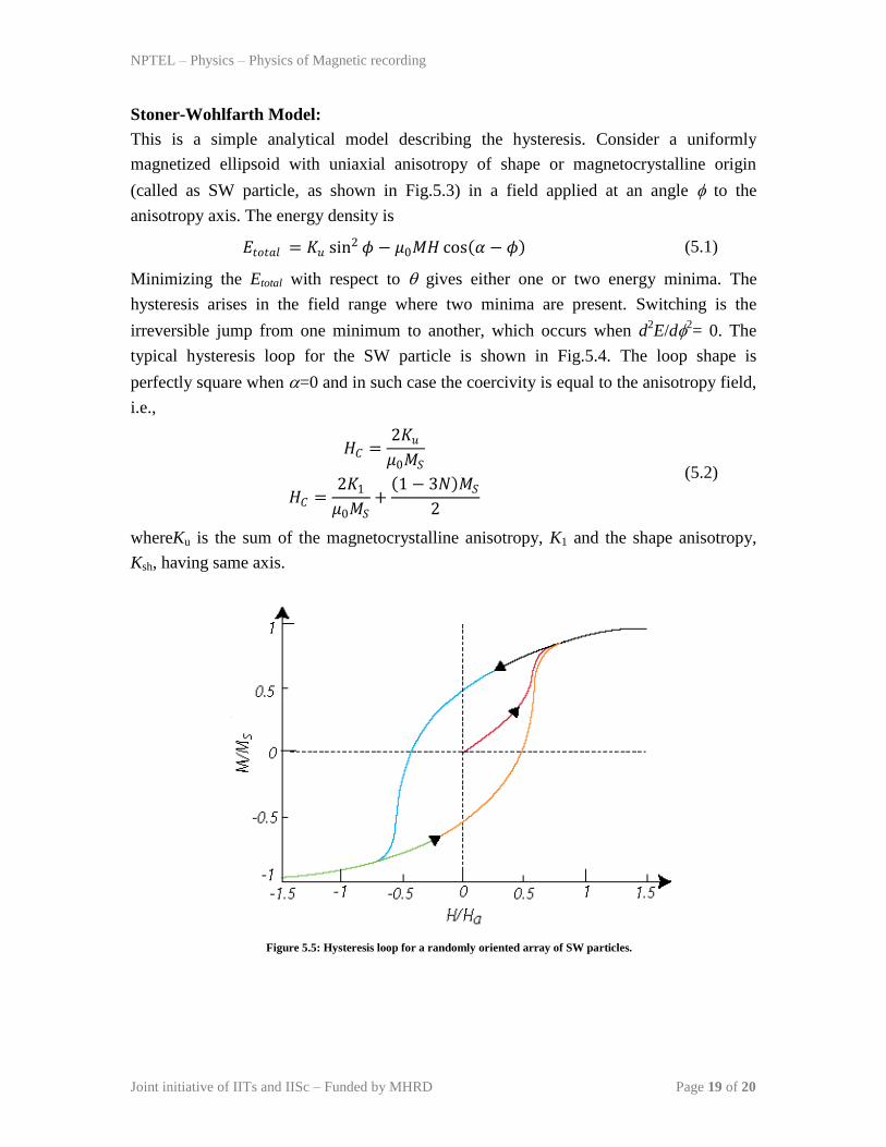
Figure 5.5: Hysteresis loop for a randomly oriented array of SW particles.
NPTEL – Physics – Physics of Magnetic recording
Joint initiative of IITs and IISc – Funded by MHRD Page 20 of 20
An array of non-interacting magnetic particles with a random distribution of anisotropy
axes is a crude model for a real polycrystalline magnet. The hysteresis loop of such
magnet is given in Fig. 5.5. The remnance for the array of particles is ½MS and the
coercivity is 0.482Ha. If the anisotropy directions are distributed at random within the
place, a case similar to particulate recording media, the remnance is 0.637MS (=2/) and
the coercivity is 0.508 Ha.
Another possible relation (Henkel plot) between two remnance curves for the system of
non-interacting particles was pointed by Wohlfarth. The remnance on the initial
magnetization curve, Mr, is obtained by applying a field H to the virgin state, and
reducing it to zero. The remnanceMrd is obtained in a reverse field after saturating the
magnetization. They are related by
2𝑀𝑟𝑖 𝐻 = 𝑀𝑟 − 𝑀𝑟𝑑 𝐻 (5.3)
The deviations from a linear plot of Mri versus Mrd, known as Henkel plot, are the
evidence for the existence of finite interacting particles.
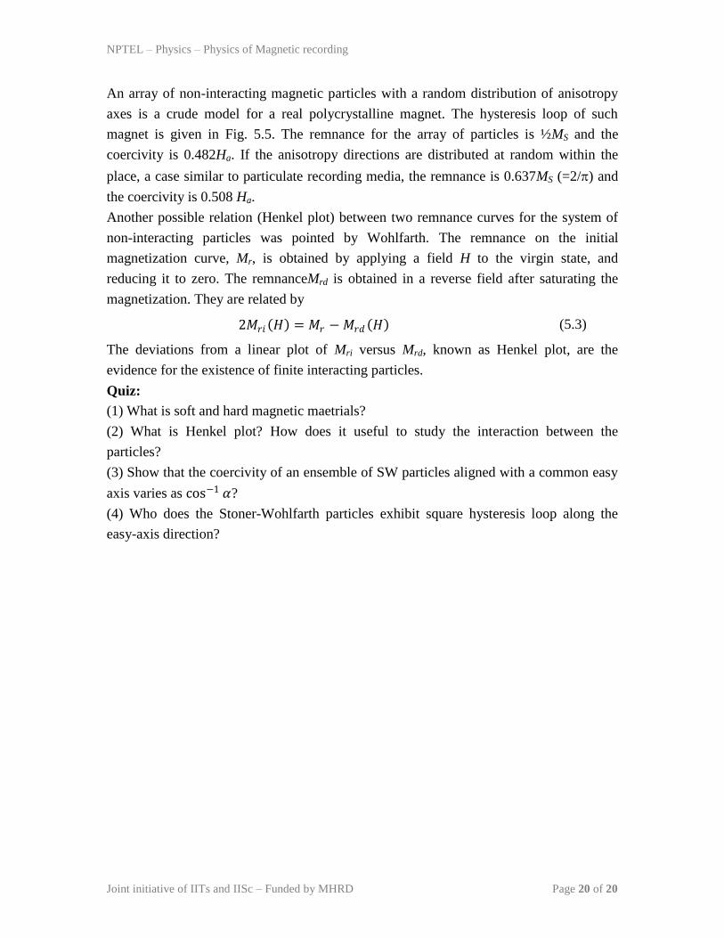
Quiz:
(1) What is soft and hard magnetic maetrials?
(2) What is Henkel plot? How does it useful to study the interaction between the
particles?
(3) Show that the coercivity of an ensemble of SW particles aligned with a common easy
axis varies as cos−1 𝛼?
(4) Who does the Stoner-Wohlfarth particles exhibit square hysteresis loop along the
easy-axis direction?
Recommended