C. Didulescu, A. Savu, C. Coşarcă, A. Negrilă
Modelling a hydrographic basin using geospatial data
- 75 -
MODELLING A HYDROGRAPHIC BASIN USING GEOSPATIAL
DATA
Caius DIDULESCU, conf. univ. dr. ing. ec ., Universitatea Tehnică de Construcţii Bucureşti,
Facultatea de Geodezie, Catedra de Topografie şi Cadastru,
Adrian SAVU, Şef lucrări univ. dr. ing., Universitatea Tehnică de Construcţii Bucureşti,
Facultatea de Geodezie, Catedra de Topografie şi Cadastru, [email protected];
Constantin COSARCA, conf. univ. dr. ing., Universitatea Tehnică de Construcţii Bucureşti,
Facultatea de Geodezie, Catedra de Topografie şi Cadastru,
Aurel NEGRILA, asist. univ. dr. ing., Universitatea Tehnică de Construcţii Bucureşti,
Facultatea de Geodezie, Catedra de Topografie şi Cadastru, [email protected];
Abstract: This article deals with the problem of modeling a river basin using geospatial
data collected by traditional methods. The raw digital terrain model for a hydrographic basin
obtained by interpolation of the point elevation data can be optimized for applications of land
improvements. The problem deals with a digital terrain model improved for water drainage
on slopes.
1. Introduction
Digital terrain models are used to study real physical or abstract phenomena, both to create
more precise images of reality, as for creating a virtual prototype that describes the structure
and behavior of natural phenomena under different conditions. Digital terrain models can be
used to develop risk maps for disaster prevention and for engineering design.
Together with the development of computer and specialized software was developed also the
possibility of approaching and solving complex problems of automation solutions for
applications that use the data field. The most practical method of making a digital terrain
model is represented through the use of contours on plans and maps. This method has the
main disadvantage that image of several contours can give information related to the
morphology of the land that allow simplified viewing of the form field.
Using contour lines specific, geomorphologic features can be represented in the various forms
of relief, which can generate a class effect. For some practical applications it is possible that
this method is sufficient, but for adequate representation of the shape of the land is necessary
to know the land. Digital terrain model aims to provide information for the entire field, having
the main advantage that it can be effectively visualized. The contour lines derive from a data
set of a digital terrain model and not vice versa.
To approximate the topographic surface of the land from the recording data can be used linear
and nonlinear interpolation method based on registered elevation points belonging to physical
surface of the land. This article presents a way to optimize the digital terrain model for water
drainage on slopes using geospatial data collected by traditional methods.
2. The design concept of the DTM The term "Digital Terrain Model” was first used in 1958 by Miller and LaFlamme and
they defined it as "a statistical representation of continuous land surface using a large number
of points whose coordinates horizontal (x, y) with altitude (z) are known, a representation
„1 Decembrie 1918” University of Alba Iulia RevCAD 15/2013
- 76 -
made in an arbitrary coordinate system.” The term Digital Terrain Model (DMT), used in
Europe, has now a broader meaning than compared with the definition given in 1958 by
Miller and LaFlamme. Thus it includes additional items such as discontinuities of the terrain
(ridges, slopes and water courses) or values of slope, aspect, visibility, etc.
Mathematical modeling of the earth's surface is the digital representation of the shape of
the ground, often complex, by a mathematical surface that approximates the topographic
surface of the land. The basic principle of modeling is to define an area of land with
coordinates x, y, h of the characteristic points of land, followed by interpolation with a
specialized software to obtain the height of any point desired for which it is known the
planimetric coordinates x and y.
3. Land surface modeling using polynomial functions
Digital terrain model is a representation of the physical land surface in a form of numerical
mathematics that involves defining a mathematical model which can be described by a
complex non-mathematical surface, such as the topographic surface that results from the
composition of the various forms of relief.
Studied in detail, the digital representations of land, reveals the complexity involved in their
implementation, due primarily to the nature of the relief.
The reconstruction of surface shape by setting new values for elevations used for interpolation
or approximation functions as well as predictive mathematical models must be flexible
enough to faithfully follow the slope and curvature of the field, taking into account all its
specific structural features.
At DTM generation using polynomial modeling, the reference points can be distributed on the
surface uniform or non-uniform, which is an advantage offered by this method.
Below is presented a modeling of land surface using non-uniformly distributed points,
respectively uniformly distributed points.
In figure below has been extracted an area from a topographic survey performed by classical
methods. Reference data were obtained with a total station and through computer programs
were determined and stored three-dimensional coordinates.
Figure 1. Topographical plan of the study area
In this regard, based on the reference set of points sampled from a surface segment,
conventional digital modeling technique apply different variations based on three different
procedures: interpolation and approximation with certain types of functions, respectively
estimation founded on statistical concepts, associated with theory of random processes
(functions).
C. Didulescu, A. Savu, C. Coşarcă, A. Negrilă
Modelling a hydrographic basin using geospatial data
- 77 -
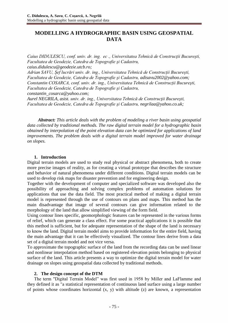
One way to create such a digital terrain model is by creating a project with a dedicated
software such as AutoCAD Land. The result is shown in the figure below.
Figure 2. The raw digital model by creating surface based on three-dimensional points
One possibility to optimize digital terrain model in this case is to create a routine that allows
the user to create an area of land that allow highlighting in detail the relief. The steps of this
process are:
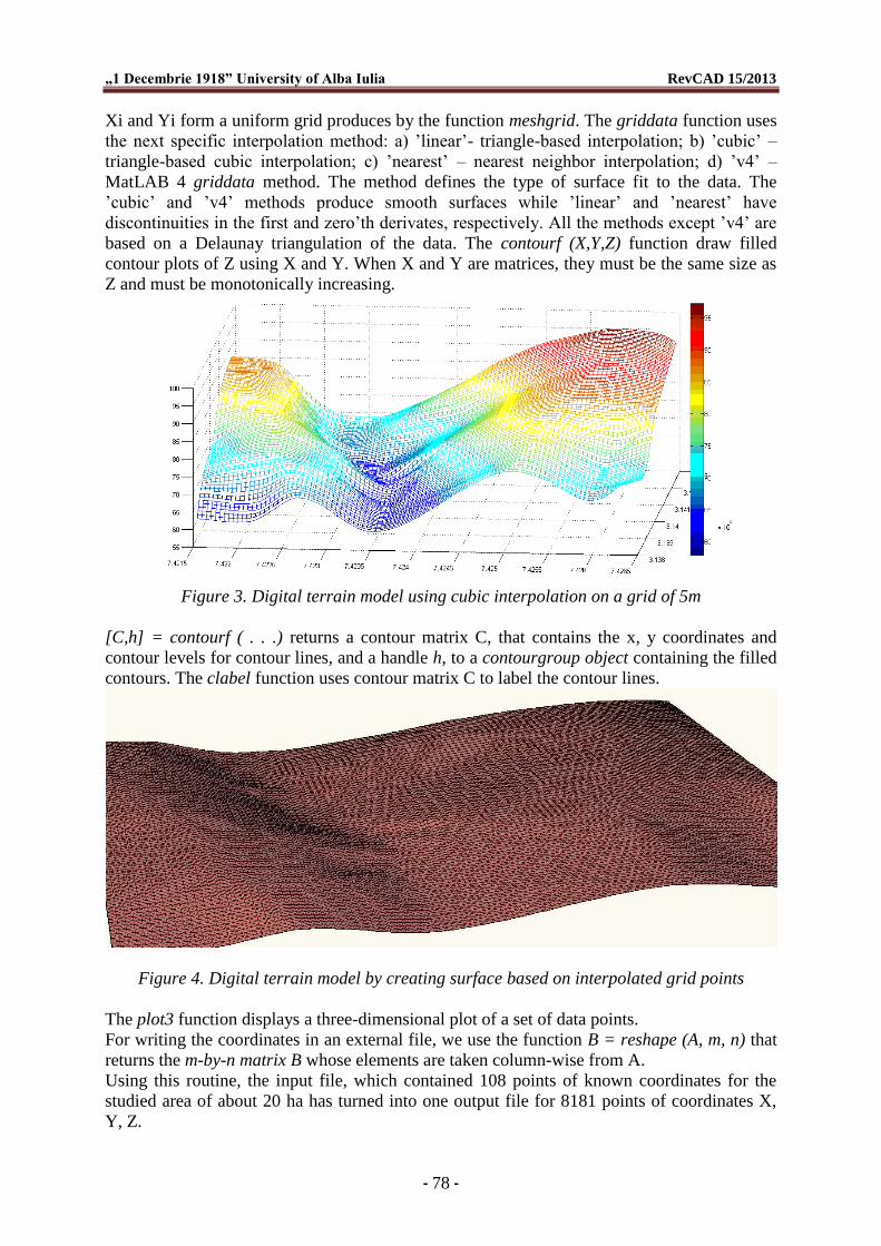
a) achieving a predefined grid with step defined by the user. In this case we set a 5m grid step;
b) generation elevations on interpolated grid by using a polynomial function, provided by
MATLAB software. We used cubic interpolation function that produces a smooth surface.
The result can be seen in Figure 3.
c) the generation of coordinates file for resulting points.
Below is the source that can be loaded into MATLAB used in this case study.
Definire grid - X max, X min, Y max, Y min, pas X si pasX
xgrid=[742150:5:742650];
ygrid=[313850:5:314250];
Generare grid
[xmesh,ymesh]=meshgrid(xgrid,ygrid);
Generare grid interpolat
zint=griddata(x,y,z,xmesh,ymesh,'cubic');
[C,h]=contourf(xmesh,ymesh,zint), grid on ;
clabel(C,h);
mesh(xmesh,ymesh,zint),hold
plot3(x,y,z,'o'), hold of
Generare ( scriere fisier) combinat
fid = fopen('grid.txt', 'w');
The routine loads coordinates x, y, z in a text file and in the next step defines grid coordinates
based on the minimum and maximum values and the grid step in the direction of X and Y.
Grid generation is performed with meshgrid function provided by Matlab.
Meshgrid function transforms the domain specified by vectors x and y into arrays X and Y,
which can be used to evaluate functions of two variables.
The griddata function Zi = griddata (x, y, z, Xi, Yi) fits a surface of the form z = f(x,y) to the
data in the nonuniforrmly spaced vectors (x, y, z). Gridddata interpolates the surface at the
points specificed by (Xi,Yi) to produce Zi. The surface always passes through the data points.
„1 Decembrie 1918” University of Alba Iulia RevCAD 15/2013
- 78 -
Xi and Yi form a uniform grid produces by the function meshgrid. The griddata function uses
the next specific interpolation method: a) ’linear’- triangle-based interpolation; b) ’cubic’ –
triangle-based cubic interpolation; c) ’nearest’ – nearest neighbor interpolation; d) ’v4’ –
MatLAB 4 griddata method. The method defines the type of surface fit to the data. The
’cubic’ and ’v4’ methods produce smooth surfaces while ’linear’ and ’nearest’ have
discontinuities in the first and zero’th derivates, respectively. All the methods except ’v4’ are
based on a Delaunay triangulation of the data. The contourf (X,Y,Z) function draw filled
contour plots of Z using X and Y. When X and Y are matrices, they must be the same size as
Z and must be monotonically increasing.
Figure 3. Digital terrain model using cubic interpolation on a grid of 5m
[C,h] = contourf ( . . .) returns a contour matrix C, that contains the x, y coordinates and
contour levels for contour lines, and a handle h, to a contourgroup object containing the filled
contours. The clabel function uses contour matrix C to label the contour lines.
Figure 4. Digital terrain model by creating surface based on interpolated grid points
The plot3 function displays a three-dimensional plot of a set of data points.
For writing the coordinates in an external file, we use the function B = reshape (A, m, n) that
returns the m-by-n matrix B whose elements are taken column-wise from A.
Using this routine, the input file, which contained 108 points of known coordinates for the
studied area of about 20 ha has turned into one output file for 8181 points of coordinates X,
Y, Z.
C. Didulescu, A. Savu, C. Coşarcă, A. Negrilă
Modelling a hydrographic basin using geospatial data
- 79 -
4. Modelling watersheds
Specific software distinguishes a number of types of watersheds. The watershed types are
based on what type of drain target the watershed has. A drain target is the location where
water flow stops or leaves the surface. Water that flows along a channel or across a surface
triangle eventually flows off the surface or it reaches a point from which there is no downhill
direction.
The region of the surface that drains to that target is called the watershed for that drain target.
Each watershed subarea is categorized as one of the following types, based on drain target:
boundary point watershed;
boundary segment watershed;
depression watershed;
multi-drain watershed.
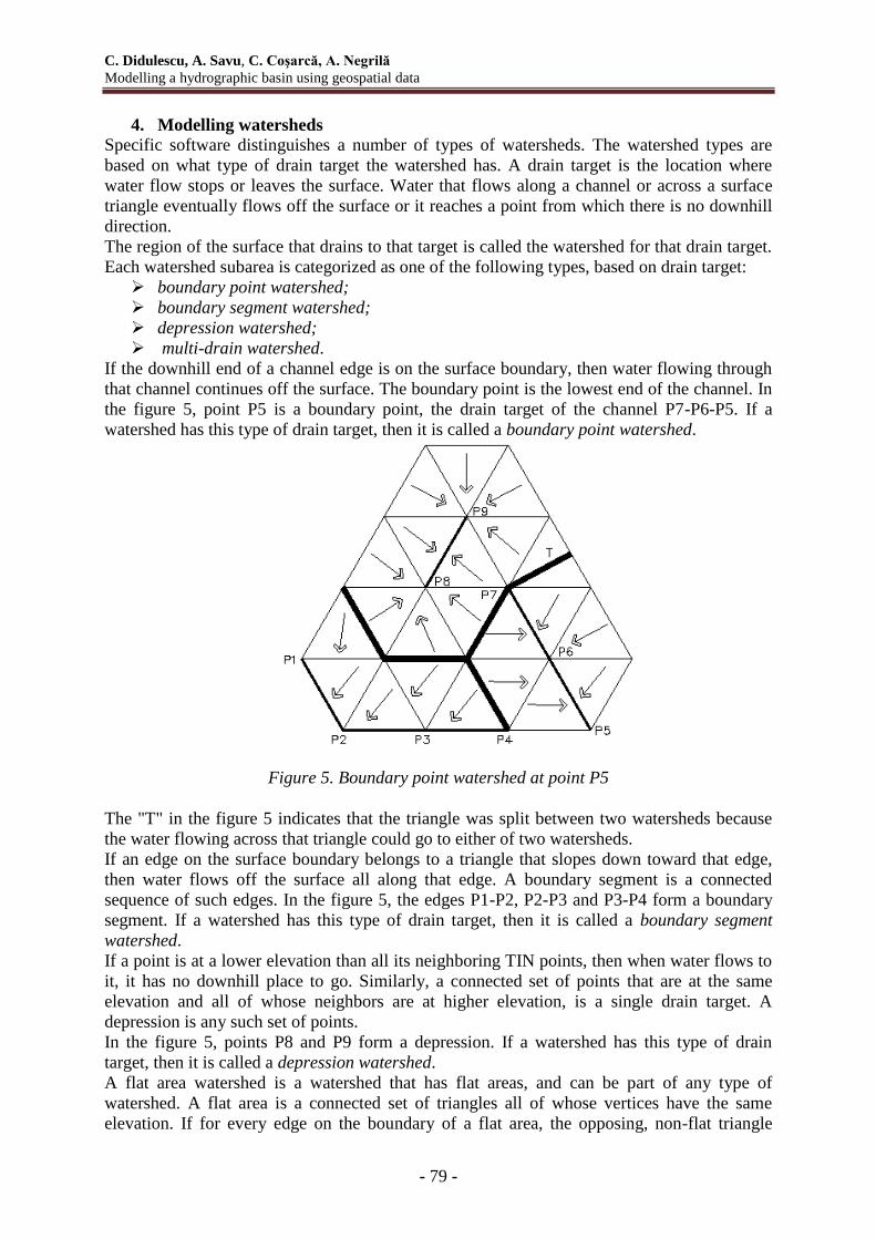
If the downhill end of a channel edge is on the surface boundary, then water flowing through
that channel continues off the surface. The boundary point is the lowest end of the channel. In
the figure 5, point P5 is a boundary point, the drain target of the channel P7-P6-P5. If a
watershed has this type of drain target, then it is called a boundary point watershed.
Figure 5. Boundary point watershed at point P5
The "T" in the figure 5 indicates that the triangle was split between two watersheds because
the water flowing across that triangle could go to either of two watersheds.
If an edge on the surface boundary belongs to a triangle that slopes down toward that edge,
then water flows off the surface all along that edge. A boundary segment is a connected
sequence of such edges. In the figure 5, the edges P1-P2, P2-P3 and P3-P4 form a boundary
segment. If a watershed has this type of drain target, then it is called a boundary segment
watershed.
If a point is at a lower elevation than all its neighboring TIN points, then when water flows to
it, it has no downhill place to go. Similarly, a connected set of points that are at the same
elevation and all of whose neighbors are at higher elevation, is a single drain target. A
depression is any such set of points.
In the figure 5, points P8 and P9 form a depression. If a watershed has this type of drain
target, then it is called a depression watershed.
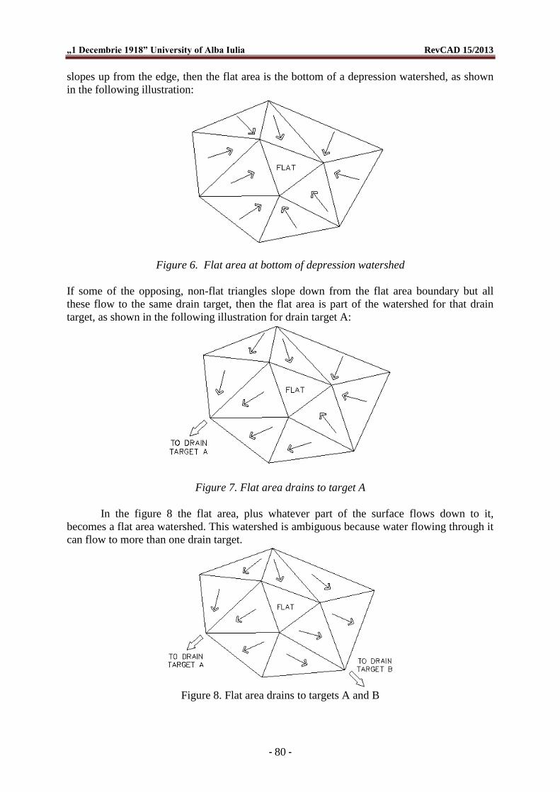
A flat area watershed is a watershed that has flat areas, and can be part of any type of
watershed. A flat area is a connected set of triangles all of whose vertices have the same
elevation. If for every edge on the boundary of a flat area, the opposing, non-flat triangle
„1 Decembrie 1918” University of Alba Iulia RevCAD 15/2013
- 80 -
slopes up from the edge, then the flat area is the bottom of a depression watershed, as shown
in the following illustration:
Figure 6. Flat area at bottom of depression watershed
If some of the opposing, non-flat triangles slope down from the flat area boundary but all
these flow to the same drain target, then the flat area is part of the watershed for that drain
target, as shown in the following illustration for drain target A:
Figure 7. Flat area drains to target A
In the figure 8 the flat area, plus whatever part of the surface flows down to it,
becomes a flat area watershed. This watershed is ambiguous because water flowing through it
can flow to more than one drain target.
Figure 8. Flat area drains to targets A and B
C. Didulescu, A. Savu, C. Coşarcă, A. Negrilă
Modelling a hydrographic basin using geospatial data
- 81 -
One type of ambiguous watershed is called a multi-drain or split channel watershed.
In the figure 9, the channel edges E2 and E3 flow to different drain targets:
Figure 9. Multi-drain or split-channel watershed
Then water flowing down edge E1 could eventually reach either of these drain targets.
In a case like this, the region that flows to edge E1 is defined as a multi-drain watershed.
A multi-drain notch watershed occurs where there is a notch in the surface, illustrated by the
flat edge created between P1 and P2 in the following illustration. This type of watershed is
called a "multi-drain" notch because water flowing into the notch could drain to drain target A
or drain target B.
Figure 10. Drain targets for multi-drain notch watershed
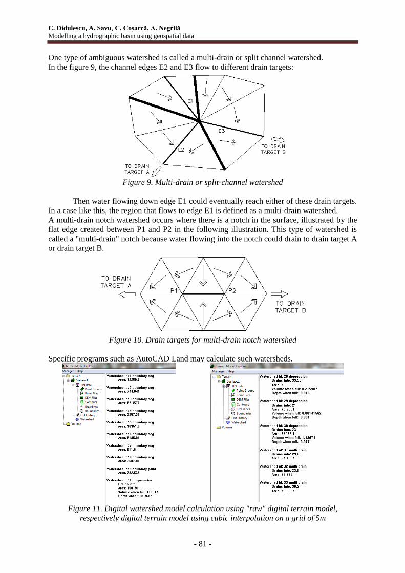
Specific programs such as AutoCAD Land may calculate such watersheds.
Figure 11. Digital watershed model calculation using "raw" digital terrain model,
respectively digital terrain model using cubic interpolation on a grid of 5m
„1 Decembrie 1918” University of Alba Iulia RevCAD 15/2013
- 82 -
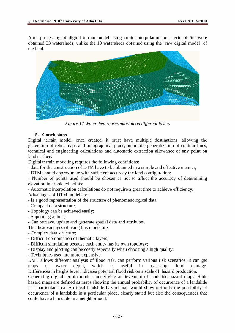
After processing of digital terrain model using cubic interpolation on a grid of 5m were
obtained 33 watersheds, unlike the 10 watersheds obtained using the "raw"digital model of
the land.
Figure 12 Watershed representation on different layers
5. Conclusions
Digital terrain model, once created, it must have multiple destinations, allowing the
generation of relief maps and topographical plans, automatic generalization of contour lines,
technical and engineering calculations and automatic extraction allowance of any point on
land surface.
Digital terrain modeling requires the following conditions:
- data for the construction of DTM have to be obtained in a simple and effective manner;
- DTM should approximate with sufficient accuracy the land configuration;
- Number of points used should be chosen as not to affect the accuracy of determining
elevation interpolated points;
- Automatic interpolation calculations do not require a great time to achieve efficiency.
Advantages of DTM model are:
- Is a good representation of the structure of phenomenological data;
- Compact data structure;
- Topology can be achieved easily;
- Superior graphics;
- Can retrieve, update and generate spatial data and attributes.
The disadvantages of using this model are:
- Complex data structure;
- Difficult combination of thematic layers;
- Difficult simulation because each entity has its own topology;
- Display and plotting can be costly especially when choosing a high quality;
- Techniques used are more expensive.
DMT allows different analysis of flood risk, can perform various risk scenarios, it can get
maps of water depth, which is useful in assessing flood damage.
Differences in heighs level indicates potential flood risk on a scale of hazard production.
Generating digital terrain models underlying achievement of landslide hazard maps. Slide
hazard maps are defined as maps showing the annual probability of occurrence of a landslide
in a particular area. An ideal landslide hazard map would show not only the possibility of
occurrence of a landslide in a particular place, clearly stated but also the consequences that
could have a landslide in a neighborhood.
C. Didulescu, A. Savu, C. Coşarcă, A. Negrilă
Modelling a hydrographic basin using geospatial data
- 83 -
Although it offers a better accuracy, the surveying methods and topographic apparatus prove
successful only if the DTM cover small areas of land necessary for applications such as
detailed projects for airports, industrial buildings, residential blocks, achieving intersections
(nodes) of paths communications, landslides hazard maps.
References:
1. Badescu O., Dumitru P., Plopeanu M., „Geoid modelling by astro-geodetic
measurements”, International Scientific Symposium GeoCAD12, Alba Iulia, 11-12
may 2012, RevCAD Journal of Geodesy and Cadaster No.13/2012, ISSN 1583-2279,
18-24 pp, Aeternitas Publishing House, 2012.
2. Didulescu Caius, Savu Adrian – „Study on the use of dem to the achievement of risk
and hazard maps”, Revista Geographia Napocensis, Anul V, nr. 1 din 2011, Academia
Română, Filiala Cluj-Napoca, http://geographianapocensis.acad-cluj.ro/
3. Didulescu Caius, Adrian Savu – „Aspects of volume calculation”, Journal of Applied
Engineering Sciences, Volume 1 (16). Issue 1, University of Oradea Publishing House,
pag. 31-34, 2013.
4. Dumitru P., Plopeanu M., Badescu O., Modelling the Romanian quasigeoid using
EGG97 model, GNSS and leveling measurements, International Scientific Symposium
GeoCAD12, Alba Iulia, 11-12 may 2012, RevCAD Journal of Geodesy and Cadaster
No.14/2013, ISSN 1583-2279, Aeternitas Publishing House, 2013.
5. P. Dumitru, M. Plopeanu, A. Jocea, A. Calin, O. Badescu, Approaches on geoid
modeling, 13th SGEM GeoConference on Informatics, Geoinformatics And Remote
Sensing, www.sgem.org, SGEM2013 Conference Proceedings, ISBN 978-619-7105-01-
8 / ISSN 1314-2704, June 16-22, 2013, Vol. 2, 57 - 64 pp, DOI:
10.5593/SGEM2013/BB2.V2/S09.008
6. P.D.Dumitru, C. Cosarca, A.Calin, Modelling the quasigeoid for the Dobrogea and
Seaside area, Romania, 1st European Conference of Geodesy & Geomatics
Engineering GENG '13, Antalya, Turkey, October 8-10, 2013, Recent Advanced in
Geodesy and Geomatics Engineering – Conference Proceedings, ISSN 2227-4359 /
ISBN 978-960-474-335-3, 140-147pp, Antalya, October 8-10, 2013.
7. P.D.Dumitru, M. Plopeanu, D.Badea, Comparative study regarding the methods of
interpolation, 1st European Conference of Geodesy & Geomatics Engineering GENG
'13, Antalya, Turkey, October 8-10, 2013, Recent Advanced in Geodesy and Geomatics
Engineering – Conference Proceedings, ISSN 2227-4359 / ISBN 978-960-474-335-3,
45-52pp, Antalya, October 8-10, 2013.
8. Hutchinson M.F. – „A new procedure for gridding elevation and stream line data with
automatic removal of spurious spits”, Journal of Hidrology, nr. 106, Elsevier Science
Publishers, pag. 211-232, 1989
9. Savu Adrian, Didulescu Caius, – „3D modelling using laser scanning technique”,
Journal of Applied Engineering Sciences, Volume 1 (16). Issue 1, University of Oradea
Publishing House, pag. 119-124, 2013.
10. LI, Z., ZHU, Q. and GOLD, C. - “Digital terrain modeling: principles and
methodology”, CRC Press. Boca Raton, 2005.
- http://www.intermap.com
- http://sapiens.revues.org/index738.html.
- http://www2.cs.uh.edu/~somalley/DemTutorial/#DEM
- http://www.geo.hunter.cuny.edu/terrain/
- http://www.environment-agency.gov.uk/default.aspx

„1 Decembrie 1918” University of Alba Iulia RevCAD 15/2013
- 84 -
- http://www.mathworks.com/index.html?s_cid=pl_homepage
- http://www.mathworks.com/pl_support
- http://www.autodesk.com/products/autodesk-autocad-civil-3d/overview
- http://usa.autodesk.com/adsk/servlet/
Recommended