Non-peer reviewed EarthArXiv preprint
【This manuscript has not been submitted to any journal and not under any peer review yet】
1
Modeling transpiration with sun-induced chlorophyll fluorescence via water use 2
efficiency and stomatal conductance 3
Huaize Feng1, Tongren Xu1, Xinlei He1, Jingxue Zhao1, Shaomin Liu1 4
1 State Key Laboratory of Earth Surface Processes and Resource Ecology, School of Natural 5
Resources, Faculty of Geographical Science, Beijing Normal University, Beijing 100875, China 6
Key Points: 7
• Transpiration can be modeled accurately by SIF observations via water use efficiency and 8
stomatal conductance methods. 9
• Mechanism models outperformed the linear models for monitoring transpiration. 10
• Air dryness has an important impact on the relationship between transpiration and SIF. 11
Abstract 12
Successfully applied in the carbon research area, sun-induced chlorophyll fluorescence (SIF) has 13
raised the interest of researchers from the water research domain. However, the mechanism 14
between SIF emitted by plants and transpiration (T) has not been fully explored. To improve the 15
understanding of the relationship between SIF and T, we developed two SIF-T models, namely the 16
WUE model and conductance model, based on carbon-water coupling framework. Hourly data 17
observation at 4 sites were used to develop and validate the model, which were covered C3 and 18
C4 plants. Compared with traditional model, results show that the developed WUE model and 19
conductance model have higher R2 and lower RMSE. The developed models further indicate the 20
potential and mechanism in estimating water flux by remotely sensed SIF observations. 21
1 Introduction 22
Evapotranspiration (ET) is not only a pipeline of the water cycle in the air but also an important 23
influence factor of energy balance as a carrier of latent heat. Previous works indicated transpiration 24
(T) occupies a dominant position in evapotranspiration [Good et al., 2015; Jasechko et al., 2013]. 25

Non-peer reviewed EarthArXiv preprint
【This manuscript has not been submitted to any journal and not under any peer review yet】
In some ecosystems, T could reach 95% of the total ET [Stoy et al., 2019]. T is also closely coupled 26
with the carbon plant productivity [Kool et al., 2014]. Therefore, an accurate understanding of the 27
spatiotemporal changes of T is crucial for understanding the substance and energy interactions 28
between the land surface and the atmosphere. 29
In this century, Sun-induced chlorophyll fluorescence (SIF) renewed the gross primary 30
production (GPP) estimation from ground to space [Frankenberg and Berry, 2018; Ryu et al., 2019; 31
Schimel et al., 2019]. Considering the connection between photosynthesis and transpiration, SIF 32
may serve as a pertinent constrain estimates for transpiration. [Alemohammad et al., 2017; Jonard 33
et al., 2020]. Recently, Empirical analysis based on ground and remote sensing SIF observation 34
showed SIF is strongly related to T, [Lu et al., 2018] reconstructed the full band SIF and exploit 35
the capacity of individual SIF bands and their combinations for deriving T with empirical linear 36
regression and Gaussian Process Regression model at Harvard Forest. [Pagán et al., 2019] used 37
radiation corrected GOME-2 SIF observations to diagnose transpiration efficiency understood as 38
the ratio between transpiration and potential evaporation worldwide. [Maes et al., 2020] 39
investigated the empirical link between SIF and T using satellite SIF (GOME-2 and OCO-2) and 40
SCOPE model at sites from FLUXNET. However, the studies mentioned above relate T with SIF 41
empirically, not mechanistically. SIF is the light signal from the excited chlorophyll a molecules 42
after absorption of photosynthetically active radiation. The information about the electron 43
transport (J) from photosystem II to photosystem I contained in SIF makes the signal a powerful 44
tool to predict GPP [Gu et al., 2019; Köhler et al., 2018; Zhang et al., 2014]. Furthermore, the 45
essential of understanding the SIF-T relationship should lie in the coupling between the carbon 46
and water cycles. 47

Non-peer reviewed EarthArXiv preprint
【This manuscript has not been submitted to any journal and not under any peer review yet】
The carbon and water cycles between the biosphere and atmosphere are strongly coupled 48
[Gentine et al., 2019]. The trade-off between photosynthesis and water vapor loss is arguably the 49
most central constraint on plant function [Wolz et al., 2017]. Water-use efficiency (WUE) and 50
stomatal conductance (gs, or canopy conductance, gc) are two key metrics of carbon - water 51
coupling. WUE is defined as the amount of carbon assimilated relative to water use [Leakey et al., 52
2019]. [Maes et al., 2020] reported WUE and related variables show a most important impact on 53
the SIF-T relation. Plants take in carbon dioxide and breath out water through stomata 54
simultaneously. Stomata played a key role in the carbon-water coupling, even the whole Earth 55
System [Berry et al., 2010]. By analyzing the empirical link of SIF and canopy conductance, [Shan 56
et al., 2019] reported the empirically linear linkage between gs and SIF data from C3 forest, 57
cropland, and grassland ecosystems, and T calculated by SIF-based conductance agreed well with 58
ET observed by flux towers. 59
Even though some studies have been conducted for T estimation based on SIF observations, 60
they usually use the empirical method. It is unclear how can WUE and gs be used to model T by 61
SIF mechanistically. In this paper, two carbon-water coupling indicators: water use efficient and 62
stomatal conductance are introduced to clarify the physical relevance between SIF and T. Using 63
the concept of these two indicators, two mechanism SIF-T models are built and tested based on 64
hourly ground observations at four sites, including two C4 and two C3 sites. The results are 65
expected to improve our understanding of the link between SIF and T. 66
2 Materials and Methods 67
2.1 Materials 68
SIF and corresponding observation (eg. meteorological variables, flux observation, and 69
vegetation indexes) are acquired at four sites including two maize field sites (Daman from Heihe 70

Non-peer reviewed EarthArXiv preprint
【This manuscript has not been submitted to any journal and not under any peer review yet】
river basin, China, DM; Huailai from Haihe river basin, China, HL), one temperate deciduous 71
forest site (Harvard Forest from AmeriFlux network, US, HF), and a subalpine conifer forest 72
(Niwot Ridge from AmeriFlux network, US, NR). The characteristics of these sites are 73
summarized in Table 1. The SIF measurements of DM and HL sites (760 nm) were conducted 74
using a tower-based automatic measurement system named “SIFSpec” [Du et al., 2018] and 75
retrieved using the 3FLD method [Liu et al., 2020]. The SIF data (745- to 758-nm) of NR were 76
from a scanning spectrometer (PhotoSpec) on the top of the 26 meters tower. SIF data in winter 77
were abandoned in this study because the subalpine trees at the NR site undergone significant 78
physiological stress during the cold climate [Magney et al., 2019]. The SIF data of HF were 79
retrieved from FluoSpec deployed about 5 m above the canopy on the top of a tower and extracted 80
by spectral fitting methods at 760 nm [Yang et al., 2015]. 81
Meteorological variables include net radiation (Rn), relative humidity and so on (See Table 82
2). Latent heat (LE) and net ecosystem exchange (NEE) are taken from flux observed by Eddy 83
Covariance towers. Gross primary production (GPP) was separated from net ecosystem exchange 84
(NEE) following [Reichstein et al., 2005] and [Lasslop et al., 2010] via the REddyProcWeb online 85
tool (https://www.bgcjena.mpg.de/bgi/index.php/Services /REddyProcWeb). Leaf area index 86
(LAI) of all four sites was acquired from the MCD15A3H dataset with 4-day and 500 m temporal-87
spatial resolution [Myneni et al., 2015] and interpolated to hourly scale on Google Earth Engine 88
[Gorelick et al., 2017]. One hour before the rainfall and six hours after the rainfall data were 89
excluded to minimize the influence of canopy interception. 90
T modeled by SIF is evaluated by TZhou partitioned from ET. [Zhou et al., 2014] proposed an 91
index called underlying water-use efficiency (uWUE) by combining the optimal stomatal behavior 92
model with Fick's law. This method was developed based on flux tower data of 14 sites, including 93

Non-peer reviewed EarthArXiv preprint
【This manuscript has not been submitted to any journal and not under any peer review yet】
the HF site, and successfully applied to Heihe River Basin [Zhou et al., 2018], including the DM 94
site. Especially, at the DM site, T/ET estimated by the uWUE method agreed with the isotope 95
method well during the peak growing season [Bai et al., 2019]. 96
2.2 WUE Model 97
SIF and GPP can both be represented in the form of light use efficiency (LUE) model: 98
SIF = APAR ΦF Ωc (1) 99
GPP = APAR LUE (2) 100
where APAR stands the photosynthetically active radiation absorbed by photosynthetic 101
pigments, ΦF is the fluorescence quantum yield, and Ω𝑐 is the probability of SIF photon escaping 102
from the canopy. Combining Eqn 1 with Eqn 2, we can obtain a linear model between SIF and 103
GPP: 104
GPP = SIFLUE
ΦF Ωc
(3) 105
where LUE is the light-use-efficiency. Based on previous works [Guanter et al., 2014; Li et al., 106
2018; Sun et al., 2017; Liu et al., 2017; Magney et al., 2019; Yang et al., 2015], the factor LUE
ΦF×Ωc 107
can be set as a constant for a specific plant type, and GPP can be calculated by SIF directly. For 108
C3 and C4 plants, WUE is relatively stable. Many works derived T from GPP by treating WUE as 109
a constant value during certain period [Scott and Biederman, 2017; Yang et al., 2015]. Under this 110
assumption T can be calculated by SIF via the following equation: 111
GPPlinear = k1 SIF (4) 112
Tlinear = k2 GPPlinear (5) 113
where k1, k2 are two parameters denoting LUE
ΦF×Ωc and WUE respectively. Eqn 5 is the theory base 114
of the empirical linear relationship between SIF and T. 115

Non-peer reviewed EarthArXiv preprint
【This manuscript has not been submitted to any journal and not under any peer review yet】
However, WUE is strongly affected by the dryness of air from leaf to ecosystem scale. The 116
relationship between GPP and T improved significantly by incorporating the effects of the vapor 117
pressure deficit (VPD) from diurnal to annual time scales [Beer et al., 2009; Zhou et al., 2014]. 118
Moreover, [Jonard et al., 2020] pointed out the atmospheric demand for water helps explaining a 119
lot variability in the SIF–T relationship at the ecosystem scale. Here we proposed a WUE model: 120
GPPWUE = k3 SIF (6) 121
TWUE = k4 VPDk5 GPPWUE (7) 122
where k3 is a parameter like k1. k4 is a parameter concluding information on water-use efficiency. 123
k5 quantifies of the non-linear effect of VPD on k4 [Lin et al., 2018]. In this work, VPD is 124
calculated from air temperature and relative humidity of air. 125
2.3 Conductance Model 126
Though the linear SIF-GPP relationship (Eqn 3) looks simple, the mechanism of the 127
parameter LUE in is complex. Φf and Ωc are relatively stable value [Guanter et al., 2014; Tol et 128
al., 2014], and LUE is often calculated by reducing potential LUE using several environmental 129
factors, such as temperature, soil moisture [Yuan et al., 2007]. Previous work had also reported the 130
hyperbolic relationship between SIF and GPP [Damm et al., 2015; Zhang et al., 2020]. Therefore, 131
the relationship between SIF and GPP is far more complicated than linear. The link between SIF 132
and GPP is because of the close relationship between SIF and electron transport rate (J) and J can 133
be derived by SIF in [Gu et al., 2019]: 134
J = a qL SIF (8) 135
Benefit from the carbon-pump mechanism, the GPP of C4 plants is linearly related to. For C4 136
plants[Collatz et al., 1992], GPP can be derived by: 137
GPPgs = J/4 =a qL SIF
4Ωc
(9) 138

Non-peer reviewed EarthArXiv preprint
【This manuscript has not been submitted to any journal and not under any peer review yet】
a is an empirical factor supposed to be a constant under ideal environments, qL is the fraction of 139
open Photosynthesis II reaction centers, indicating the 'traffic jam' in the electron transport 140
pathway from Photosystem II to Photosystem I. Note that, the Eqn 8 is designed for broadband 141
SIF for PSII. In this paper, single NIR band SIF is used instead by assuming a linear relationship 142
between single-band SIF and full band SIF. qL ranges from 0-1 and decreases with increased PAR 143
[Baker, 2008; Gu et al., 2019]. In this paper, qL is derived by: 144
qL = exp(−βPAR) (10) 145
𝛽 is a parameter denoting the sensitivity of qL to the illumination. Due to data restrictions, Ω𝑐 for 146
the near-infrared band SIF was set as a constant in our study. gs for C4 plants is derived by inserting 147
Eqn into the famous Ball-Berry model [Ball et al., 1987]: 148
gs = m a qL SIF
4ΩcRh/Ca + g0 (11) 149
where m is an empirical slope parameter, which is often treated as a constant for a specific 150
ecosystem [Miner et al., 2017]. Ca is the ambient carbon dioxide concentration and g0 is the 151
minimum conductance which is set as 0. Lack of an efficient mechanism gathering CO2 from the 152
air, C3 plants much more rely on the stomata to absorb CO2 for the Calvin cycle. For C3 plants, 153
the relationship between SIF and GPP is also affected by the dark reactions. The relationship 154
between GPP and SIF for C3 can be expressed by [Gu et al., 2019]: 155
GPPgs = aCi − Γ∗
4Ci + 8Γ∗qL SIF
1
Ωc
(12) 156
Ci is the intercellular CO2 concentration. Γ∗ is the CO2 compensation point in the absence of 157
mitochondrial respiration, which can be set as a constant for specific plant type or calculated by 158
air temperature [Katul et al., 2010]. Ci can be eliminated by combining Eqn 12 with Fick's law 159
GPP = gs × (Ci − Ca), then we have: 160
Non-peer reviewed EarthArXiv preprint
【This manuscript has not been submitted to any journal and not under any peer review yet】
GPPgs = aGPP/gs + Ca − Γ∗
4(GPP/gs + Ca) + 8Γ∗qL SIF
1
Ωc
(13) 161
gs and GPPgs can be solved under the constraining of the optimality theory of stomatal behavior. 162
[Cowan and GD, 1977; Katul et al., 2010; Way et al., 2014]. According to this theory, plants tend 163
to adapt stomata to minimize the cost of water while maximizing carbon assimilation: 164
f(gs) = GPP − λ ET ≈ GPP − 1.6λ gs VPD/P (14) 165
δf(gs)/δ(gs) = 0 (15) 166
𝜆 represents the marginal water cost of carbon assimilation. P is the air pressure. If we incorporate 167
Eqn 13, 14, and 15, gs can be expressed as the function 𝓕 of SIF, qL, 𝜆, Γ, VPD and Ca: 168
gs = 𝓕(SIF, qL, λ, Γ, VPD, Ca) 169
= −a SIF qL(4Γ−Ca)
4(2Γ+Ca)2 +a SIF qL(2Γ+Ca−3.2λ VPD)√3.2λ VPD Γ(Ca−Γ)(2Γ+Ca−1.6VPDλ)
6.4λ VPD(2Γ+Ca)2(2Γ+Ca−1.6λ VPD) (16) 170
Finally, with SIF-based gs, T can be calculated by the two-source Penman-Monteith method 171
[Leuning et al., 2008]: 172
Ac = Rn × [1 − exp(−0.5LAI)/ cos(SZA)] (17) 173
Tgs =Δ Ac + ρ Cp VPD ga
Δ + γ (1 +gags)
(18) 174
Eqn 17 is the simple one-dimensional Beer's law model. Ac is the available energy of the canopy 175
layer, Rn is net radiation, LAI is the leaf area index and SZA is the sun zenith angle. For Eqn 18, 176
Δ is the rate of change of vapor pressure with temperature, γ is the psychrometric constant, Cp is 177
the specific heat of air; ρ is the density of liquid water, and ga is aerodynamic conductance. 178
2.3 Model Calibration 179
Parameters of both the WUE model and the conductance model need to be calibrated (see 180
Table 3). GPP and the water balance framework are used here to constrain the models. Total ET 181

Non-peer reviewed EarthArXiv preprint
【This manuscript has not been submitted to any journal and not under any peer review yet】
observed by eddy covariance measurement is composed of plant transpiration (T) and soil 182
evaporation (LEs): 183
LE = T + LEs (19) 184
LEs can be calculated by soil available energy (see Table 2).Considering the nonlinearity and 185
complicity of the models, the shuffled complex evolution (SUE-UA) algorithm [Duan et al., 1994] 186
is employed to fit parameters by maximizing the cost function G: 187
G = 0.4NSE(GPPob, GPPmodel) + 0.6NSE(LEob, LEmodel) (20) 188
where NSE is the Nash-Sutcliffe efficiency coefficient. The subscript ob means observed values 189
and variables with a subscript model mean values are derived by models described above. All model 190
estimations and statistical analyses were performed with Python 3.8.3 [Harris et al., 2020; Herman 191
and Usher, 2017; Houska et al., 2015]. The description and calculation of all variables mentioned 192
above are listed in Table 2. 193
3 Results 194
3.1 Performance of SIF- T model 195
196
Scatter plots between reference TZhou and T modeled by SIF are shown in Figure 1 (upper 197
row). In general, both the WUE method and the conductance method improve the ability of SIF in 198
modeling T. Compared with simple linear regression with R2 = 0.51 and RMSE = 78.05 W/m2, the 199
WUE model has 10% higher R2 = 0.56 and 2% lower RMSE = 76.24 W/m2, while the conductance 200
model has 39% higher R2 = 0.71 and 30% lower RMSE = 54.50 W/m2. The linear model and the 201
WUE model tend to overestimate T at the high values area, while most points of Tgs fall near the 202
1:1 line. 203
The reference TZhou may have considerable uncertainty. Plants do not always keep a specific 204
response (square root) to VPD like described in Zhou’s method. Moreover, in some ecosystems, 205

Non-peer reviewed EarthArXiv preprint
【This manuscript has not been submitted to any journal and not under any peer review yet】
the soil evaporation can not be ignored even in the peak growing season [Li et al., 2019; Stoy et 206
al., 2019]. Here we also compared the LE derived by three SIF-T models with LE observed by 207
eddy covariance in Fig1 (lower row). The linear model, WUE model and conductance model have 208
R2 = 0.56, 0.61 and 0.73 and RMSE = 94.60, 91.20 and 68.07 W/m2 respectively. Same as 209
compared with TZhou, the conductance model outperforms the other two models with the highest 210
coefficients of determination and the lowest RMSE. The WUE model also has better performance 211
than the widely used linear model. 212
213
214 Figure 1. Relationship of T modeled by SIF and reference latent heat (Hourly). Colors indicate 215
the density of points (from sparse to dense: blue to red). R2 denotes the coefficient of determination. 216
The unit of root-mean-square deviation (RMSE) is W/m2. Black line denotes 1:1 line. 217
218
The performance of three models at different sites is shown in Table 4. When compared to 219
TZhou, the conductance model shows the best performance at DM and HF sites with much higher 220
R2 = 0.84, 0.62, and lower RMSE = 47.98, 77.43 W/m2 respectively. The linear model shows the 221
Non-peer reviewed EarthArXiv preprint
【This manuscript has not been submitted to any journal and not under any peer review yet】
best performance with R2 = 0.58 and RMSE = 50.94 W/m2 at the HL site. The WUE model 222
outperforms other models at the NR site. When compared to LE observed by eddy covariance, the 223
conductance model shows outstanding performance at all four sites. Besides, the WUE model has 224
the lowest RMSE = 67.38 W/m2 at the NR site. 225
3.2 Sensitivity analysis of variables in two models 226
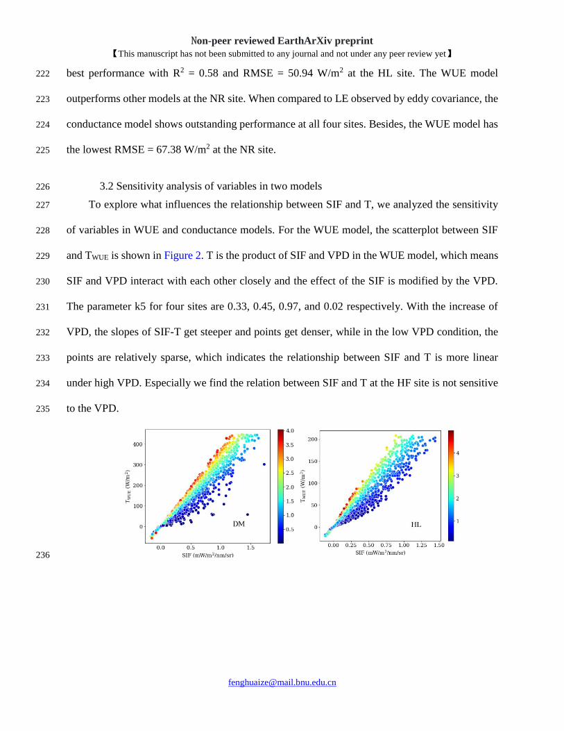
To explore what influences the relationship between SIF and T, we analyzed the sensitivity 227
of variables in WUE and conductance models. For the WUE model, the scatterplot between SIF 228
and TWUE is shown in Figure 2. T is the product of SIF and VPD in the WUE model, which means 229
SIF and VPD interact with each other closely and the effect of the SIF is modified by the VPD. 230
The parameter k5 for four sites are 0.33, 0.45, 0.97, and 0.02 respectively. With the increase of 231
VPD, the slopes of SIF-T get steeper and points get denser, while in the low VPD condition, the 232
points are relatively sparse, which indicates the relationship between SIF and T is more linear 233
under high VPD. Especially we find the relation between SIF and T at the HF site is not sensitive 234
to the VPD. 235
236

Non-peer reviewed EarthArXiv preprint
【This manuscript has not been submitted to any journal and not under any peer review yet】
237
Figure 2. Scatter plot between SIF and T modeled by the WUE method. The vapor pressure deficit 238
(VPD) has the unit kPa. 239
Atmospheric dryness is also important in modeling the stomatal behavior by SIF. For C4 240
plants, relative humidity is used to describe the response of stomatal conductance to air dryness in 241
the empirical Ball Berry model. For C3 plants, we investigated the sensitivities of different 242
variables in the gs model 𝓕 by RBD-FAST-Random Balance Designs Fourier Amplitude 243
Sensitivity Test [Tarantola et al., 2006]. According to Figure 3, 𝓕 is sensitive to VPD, λ, SIF, 244
and qL. VPD exhibits the highest first-order sensitivities with values equaling 0.09, which is much 245
higher than SIF with value 0.05. The marginal water use efficiency λ also plays an important role 246
in 𝓕 with sensitivity value equaling 0.07. The fraction of open Photosynthesis II reaction centers 247
qL is as important as SIF (1st-order sensitivity: 0.04), which is due to the electron transport rate J 248
is the product of SIF and qL (Eqn 4). What’s more, the gs model is not sensitive to air temperature 249
and ambient carbon dioxide concentration. However, VPD used here is calculated by temperature 250
and relative humidity of the air. The temperature information contained in VPD (R2 of Ta-VPD is 251
0.48) may impair the role of air temperature in the model. In this paper, qL is calculated by a simple 252
empirical equation of PAR. In fact, qL is also related to the dark reaction but poorly studied [Baker, 253
2008; Gu et al., 2019]. More researches about qL will improve our understanding of the 254
relationship between SIF and J, further the SIF-GPP and SIF-T relationships. 255

Non-peer reviewed EarthArXiv preprint
【This manuscript has not been submitted to any journal and not under any peer review yet】
256
Figure 3. Sensitivity analysis of variables in the stomatal conductance model 𝓕 of C3 plants. The 257
height of bars shows the 1st order sensitivities of different variables. 258
4 Discussion 259
Above all, the assumptions of carbon-water coupling may affect our results. Compared with 260
the linear model, though the influence of VPD on water-use efficiency is included in the WUE 261
model, soil moisture, hydraulic conductance, and other environmental variables can influence 262
water-use efficiency independently [Leakey et al., 2019; Lin et al., 2015; Liu et al., 2020]. For the 263
conductance model, plants under stress or competition tend to change the optimal stomatal 264
conductance behavior [Wolf et al., 2016]. The carbon-water economy is also influenced by traits 265
of plants and environmental variables [Bloom et al., 1985; Buckley et al., 2017]. This concept is 266
out of the scope of this paper, but a more physiologically based water-carbon coupling framework 267
will improve the models from the bottom up. 268
Due to the absence of direct measurements of transpiration during the research period, three 269
models were calibrated by the water budget balance framework, which might introduce uncertainty 270
to parameters, further the performance of the models. Net radiation is separated into energy 271
intercepted by canopy and soil available energy by 1D Beer's law. The simple structure of Beer's 272
law can introduce great uncertainty, especially for heterogeneity canopy and plants with leaves 273
highly anisotropic leaves in the azimuthal direction [Ponce De León and Bailey, 2019]. In the 274
conductance model, canopy available energy is also used to estimate transpiration in the two-275

Non-peer reviewed EarthArXiv preprint
【This manuscript has not been submitted to any journal and not under any peer review yet】
source Penman-Monteith model. So, the conductance model is more sensitive to the partition of 276
energy, in other words, suffers more uncertainty from Beer’s law. Uncertainty of input data might 277
also affect our results. Firstly, VPD in the air was used to assess the aridity stress by assuming the 278
canopy and the atmosphere are fully coupled. Yet, ecosystems (DM, HL, and HF) with dense 279
closed canopy tend to decouple from the air [De Kauwe et al., 2017; Li et al., 2019; Lin et al., 280
2018]. As both the WUE model and conductance model shows great sensitivity to VPD, using 281
VPD at the leaf scale could help to improve the performance of the SIF-T relationship. Secondly, 282
SIF data from four sites are measured by different instruments and derived by different methods 283
as mentioned above. Moreover, the FOV and heights of the observation systems vary among sites. 284
The emerge of remotely sensed SIF will fill the gap of the difference in the observation data. Last 285
but not the least, the canopy-scale SIF was directly used to model transpiration due to data 286
restriction. Nevertheless, recent papers indicated the relationship between SIF and GPP is strongly 287
affected by the structure of the canopy [Liu et al., 2019; Zeng et al., 2019]. We suggest 288
downscaling of SIF from the canopy scale to the photosystem scale may improve the performance 289
of the model. 290
Data from four sites were used to test the performance of the models. It is inadequate to show 291
the real potential of two models. With more and more in-situ observations from different 292
ecosystems, understanding of the underlying mechanism between SIF and T will be deepened. 293
Recently, SIF products with higher temporal-spatial resolution from different satellites, different 294
bands [Du et al., 2018; Köhler et al., 2018; Köhler et al., 2020], and derivative products based on 295
machine learning [Li and Xiao, 2019; Ma et al., 2020; Yu et al., 2019; Zhang et al., 2018] became 296
available. WUE model and conductance model can be easily combined with remote sensing ET/T 297
model like TSEB [Norman et al., 1995; Song et al., 2016] and PML ([Zhang et al., 2019] or used 298

Non-peer reviewed EarthArXiv preprint
【This manuscript has not been submitted to any journal and not under any peer review yet】
for assimilating SIF into a land surface model. With these data and models in this paper, estimating 299
T via SIF at the big scale becomes promising. 300
5 Conclusion 301
In this study, in-situ hourly SIF and corresponding meteorological variables, eddy covariance 302
observation and vegetation indexes at C3 and C4 sites were collected. Two SIF-T models based 303
on water-use efficiency and stomatal conductance were developed and tested upon this data. Both 304
models outperformed simple linear analysis. The WUE model has 10% higher R2 and 2% lower 305
RMSE, while the conductance model has the 39% higher R2 and 30% lower RMSE. Our results 306
indicate the SIF-T relationship depends on air dryness. These two carbon-water coupling models 307
can be easily combined with state-of-the-art remote sensing models or land process models. 308
Moreover, with the emergency of high temporal-spatial resolution SIF data, SIF will not only be a 309
powerful proxy for carbon flux but also water flux at the planetary scale. 310
311
312
Table 1. Summary of the stations used to build models. 313 Latitude Longitude Period Land Cover Reference
DM 100.37°E 38.85°N 2017.6 – 2017.9;
2018.6 – 2018.9 Maize (C4) [Liu et al., 2018; Liu et al., 2019]
HL 115.78°E 40.33°N 2017.7 – 2017.10; 2018.7 – 2018.10
Maize (C4) [Liu et al., 2013; Liu et al., 2019]
NR 105.55°W 40.03°N 2017.6-2017.9; 2018.6-2018.7
Mixed temperate forest (C3)
[Burns et al., 2015; Magney et al., 2019]
HF 72.17° W 42.54°N 2013.6-2013.11 Evergreen needle leaf
forest(C3)
[Munger W, 2020; Yang et al.,
2015]
314
Table 2. Input and intermediate variables. AWS denotes auto weather station. FAO indicates the 315
computation methods of the variable is from http://www.fao.org. 316
Variables Unit Description Source Remarks
𝐂𝐚 μmol/mol ambient CO2
concentration Observation
Eddy
covariance
Cp J/Kg/K specific heat of air 1013 FAO

Non-peer reviewed EarthArXiv preprint
【This manuscript has not been submitted to any journal and not under any peer review yet】
LEs W/m2 Soil evaporation fΔ(Rn − Ac)
Δ + γ
[Fisher et
al., 2008]
f - Soil evaporation constraint SM/(SMmax − SMmin) -
ga m/s Aerodynamic conductance 1
𝑣/(𝑢 ∗)2 + 6.2(𝑢 ∗)−2/3
[Monteith
and
Unsworth,
2013]
GPPob μmol/m2/s Gross primary production Separated from NEE observed by
eddy covariance
[Lasslop et
al., 2010;
Reichstein et
al., 2005]
LE W/m2 Latent heat Observation Eddy
covariance
PAR W/m2 photosynthetically active
radiation Observation AWS
P kPa Air Pressure Observation AWS
qL -
Fraction of open
Photosynthesis II reaction
centers
exp(−β PAR) This paper
Rh - Relative humidity Observation AWS
Rn W/m2 Net radiation Observation AWS
SIF mW/m2/sr/nm Sun-induced chlorophyll
fluorescence Observation -
SM % Soil moisture Observation
Thermal
Dissipation
Probe
Ta °C Air temperature Observation AWS
𝐮∗ m/s Friction Velocity Observation Eddy
covariance
v m/s Wind speed Observation AWS
VPD kPa Vapor pressure deficit (100 − Rh)/100 × 0.6108
× exp(17.27 Ta/(Ta + 237.3)) FAO
𝚫 kPa/K Slope of saturation vapor
pressure curve
(2503 exp(17.27 Ta/(Ta
+ 237.3)))
/((Ta
+ 237.3)2)
FAO
𝛄 kPa/K psychrometric constant 0.665 × 0.001P FAO
𝚪 μmol/mol
CO2 compensation point
in the absence of
mitochondrial
36.9 + 1.18(Ta − 25) +
0.036(Ta − 25)2 for C3; 0 for C4
[Katul et al.,
2010]
𝛒𝐚 kg/m3 Air density 1.292 − 0.00428 Ta FAO
317

Non-peer reviewed EarthArXiv preprint
【This manuscript has not been submitted to any journal and not under any peer review yet】
Table 3. Parameters needed to be calibrated. 318
319
Parameter Lower Upper Reference
Linear model
K1 5 50 [Liu et al., 2017; Sun et al., 2017]
K2 3 50 [Huang et al., 2016]
WUE model
K3 5 50 [Liu et al., 2017; Sun et al., 2017]
K4 3 30 [Zhou et al., 2015]; This paper
K5 0 1 [Lin et al., 2018]
Conductance
model (C4)
𝛽 0 0.001 This paper; [Gu et al., 2019]
a 10 300 This paper
m 2.5 8.8 [Miner et al., 2017]
Conductance
model (C3)
𝛽 0 0.01 This paper; [Gu et al., 2019; Katul et al.,
2010]
a 10 300 This paper
λ 10 200 [Cowan and GD, 1977; Katul et al.,
2010]
320
Table 4. Coefficient of determination (R2) and root mean square error (RMSE) at different sites. 321
Best values are marked with the bold font. 322
Reference DM HL NR HF
R2 RMSE R2 RMSE R2 RMSE R2 RMSE
Tlinear
TZhou
0.46 104.25 0.58 50.94 0.49 35.32 0.45 70.66
TWUE 0.55 99.11 0.55 53.66 0.69 29.26 0.45 71.80
Tgs 0.84 47.98 0.57 54.79 0.46 41.27 0.62 77.43
LElinear
LE
0.56 119.97 0.52 67.69 0.27 68.69 0.44 81.92
LEWUE 0.55 114.20 0.55 66.71 0.36 67.38 0.44 84.87
LEgs 0.87 69.36 0.60 64.53 0.40 68.82 0.55 70.71
323
References: 324
Alemohammad, S. H., et al. (2017), Water, Energy, and Carbon with Artificial Neural Networks (WECANN): a 325
statistically based estimate of global surface turbulent fluxes and gross primary productivity using solar-induced 326
fluorescence, BIOGEOSCIENCES, 14(18), 4101-4124. 327
Bai, Y., et al. (2019), Quantifying plant transpiration and canopy conductance using eddy flux data: An underlying 328
water use efficiency method, AGR FOREST METEOROL, 271, 375-384. 329
Baker, N. R. (2008), Chlorophyll Fluorescence: A Probe of Photosynthesis In Vivo, ANNU REV PLANT BIOL, 59(1), 330
89-113. 331
Ball, J. T., et al. (1987), A model predicting stomatal conductance and its contribution to the control of photosynthesis 332
under different environmental conditions, in Progress in photosynthesis research, edited, pp. 221-224, Springer. 333
Beer, C., et al. (2009), Temporal and among-site variability of inherent water use efficiency at the ecosystem level, 334
GLOBAL BIOGEOCHEM CY, 23(2), n/a-n/a. 335
Berry, J. A., et al. (2010), Stomata: key players in the earth system, past and present, CURR OPIN PLANT BIOL, 336
13(3), 232-239. 337
Bloom, A. J., et al. (1985), Resource limitation in plants-an economic analogy, Annual review of Ecology and 338

Non-peer reviewed EarthArXiv preprint
【This manuscript has not been submitted to any journal and not under any peer review yet】
Systematics, 16(1), 363-392. 339
Buckley, T. N., et al. (2017), Optimal plant water economy, Plant, Cell & Environment, 40(6), 881-896. 340
Burns, S. P., et al. (2015), The influence of warm-season precipitation on the diel cycle of the surface energy balance 341
and carbon dioxide at a Colorado subalpine forest site, BIOGEOSCIENCES, 12(23), 7349-7377. 342
Collatz, G. J., et al. (1992), Coupled photosynthesis-stomatal conductance model for leaves of C4 plants, FUNCT 343
PLANT BIOL, 19(5), 519-538. 344
Cowan, I. R., and F. GD (1977), Stomatal function in relation to leaf metabolism and environment. 345
Damm, A., et al. (2015), Far-red sun-induced chlorophyll fluorescence shows ecosystem-specific relationships to 346
gross primary production: An assessment based on observational and modeling approaches, REMOTE SENS 347
ENVIRON, 166, 91-105. 348
De Kauwe, M. G., et al. (2017), Ideas and perspectives: how coupled is the vegetation to the boundary layer? 349
BIOGEOSCIENCES, 14(19), 4435-4453. 350
Du, S., et al. (2018), Retrieval of global terrestrial solar-induced chlorophyll fluorescence from TanSat satellite, SCI 351
BULL, 63(22), 1502-1512. 352
Duan, Q., et al. (1994), Optimal use of the SCE-UA global optimization method for calibrating watershed models, J 353
HYDROL, 158(3-4), 265-284. 354
Fisher, J. B., et al. (2008), Global estimates of the land–atmosphere water flux based on monthly AVHRR and 355
ISLSCP-II data, validated at 16 FLUXNET sites, REMOTE SENS ENVIRON, 112(3), 901-919. 356
Frankenberg, C., and J. Berry (2018), Solar induced chlorophyll fluorescence: Origins, relation to photosynthesis and 357
retrieval. 358
Gentine, P., et al. (2019), Coupling between the terrestrial carbon and water cycles—a review, ENVIRON RES LETT, 359
14(8), 83003. 360
Good, S. P., et al. (2015), WATER RESOURCES. Hydrologic connectivity constrains partitioning of global terrestrial 361
water fluxes, SCIENCE, 349(6244), 175-177. 362
Gorelick, N., et al. (2017), Google Earth Engine: Planetary-scale geospatial analysis for everyone, REMOTE SENS 363
ENVIRON, 202, 18-27. 364
Gu, L., et al. (2019), Sun-induced Chl fluorescence and its importance for biophysical modeling of photosynthesis 365
based on light reactions, NEW PHYTOL, 223(3), 1179-1191. 366
Guanter, L., et al. (2014), Global and time-resolved monitoring of crop photosynthesis with chlorophyll fluorescence, 367
Proceedings of the National Academy of Sciences, 111(14), E1327-E1333. 368
Harris, C. R., et al. (2020), Array programming with NumPy, NATURE, 585(7825), 357-362. 369
Herman, J., and W. Usher (2017), SALib: an open-source Python library for sensitivity analysis, Journal of Open 370
Source Software, 2(9), 97. 371
Houska, T., et al. (2015), SPOTting model parameters using a ready-made python package, PLOS ONE, 10(12), 372
e145180. 373
Huang, M., et al. (2016), Seasonal responses of terrestrial ecosystem water-use efficiency to climate change, GLOBAL 374
CHANGE BIOL, 22(6), 2165-2177. 375
Jasechko, S., et al. (2013), Terrestrial water fluxes dominated by transpiration, NATURE, 496(7445), 347-350. 376
Jonard, F., et al. (2020), Value of sun-induced chlorophyll fluorescence for quantifying hydrological states and fluxes: 377
Current status and challenges, AGR FOREST METEOROL, 291, 108088. 378
Katul, G., et al. (2010), A stomatal optimization theory to describe the effects of atmospheric CO2 on leaf 379
photosynthesis and transpiration, ANN BOT-LONDON, 105(3), 431-442. 380
Köhler, P., et al. (2018), Global Retrievals of Solar‐Induced Chlorophyll Fluorescence With TROPOMI: First 381
Results and Intersensor Comparison to OCO‐2, GEOPHYS RES LETT, 45(19), 10, 410-456, 463. 382
Köhler, P., et al. (2020), Global Retrievals of Solar‐Induced Chlorophyll Fluorescence at Red Wavelengths With 383
TROPOMI, GEOPHYS RES LETT, 47(15). 384
Kool, D., et al. (2014), A review of approaches for evapotranspiration partitioning, AGR FOREST METEOROL, 184, 385
56-70. 386
Lasslop, G., et al. (2010), Separation of net ecosystem exchange into assimilation and respiration using a light response 387
curve approach: critical issues and global evaluation, GLOBAL CHANGE BIOL, 16(1), 187-208. 388
Leakey, A., et al. (2019), Water Use Efficiency as a Constraint and Target for Improving the Resilience and 389
Productivity of C3 and C4 Crops, ANNU REV PLANT BIOL, 70, 781-808. 390
Leuning, R., et al. (2008), A simple surface conductance model to estimate regional evaporation using MODIS leaf 391
area index and the Penman-Monteith equation, WATER RESOUR RES, 44(10). 392
Li, X., et al. (2018), Solar-induced chlorophyll fluorescence is strongly correlated with terrestrial photosynthesis for 393

Non-peer reviewed EarthArXiv preprint
【This manuscript has not been submitted to any journal and not under any peer review yet】
a wide variety of biomes: First global analysis based on OCO-2 and flux tower observations, GLOBAL CHANGE 394
BIOL, 24(9), 3990-4008. 395
Li, X., et al. (2019), A simple and objective method to partition evapotranspiration into transpiration and evaporation 396
at eddy-covariance sites, AGR FOREST METEOROL, 265, 171-182. 397
Li, X., and J. Xiao (2019), A Global, 0.05-Degree Product of Solar-Induced Chlorophyll Fluorescence Derived from 398
OCO-2, MODIS, and Reanalysis Data, REMOTE SENS-BASEL, 11(5), 517. 399
Lin, C., et al. (2018), Diel ecosystem conductance response to vapor pressure deficit is suboptimal and independent 400
of soil moisture, AGR FOREST METEOROL, 250-251, 24-34. 401
Lin, Y., et al. (2015), Optimal stomatal behaviour around the world, NAT CLIM CHANGE, 5(5), 459-464. 402
Liu, L., et al. (2017), Directly estimating diurnal changes in GPP for C3 and C4 crops using far-red sun-induced 403
chlorophyll fluorescence, AGR FOREST METEOROL, 232, 1-9. 404
Liu, S., et al. (2018), The Heihe Integrated Observatory Network: A Basin-Scale Land Surface Processes Observatory 405
in China, VADOSE ZONE J, 17(1), 180021-180072. 406
Liu, S. M., et al. (2013), Measurements of evapotranspiration from eddy-covariance systems and large aperture 407
scintillometers in the Hai River Basin, China, J HYDROL, 487, 24-38. 408
Liu, X., et al. (2019), Downscaling of solar-induced chlorophyll fluorescence from canopy level to photosystem level 409
using a random forest model, REMOTE SENS ENVIRON, 231, 110772. 410
Liu, X., et al. (2019), Atmospheric Correction for Tower-Based Solar-Induced Chlorophyll Fluorescence Observations 411
at O2-A Band, REMOTE SENS-BASEL, 11(3), 355. 412
Liu, X., et al. (2020), Improving the potential of red SIF for estimating GPP by downscaling from the canopy level to 413
the photosystem level, AGR FOREST METEOROL, 281, 107846. 414
Liu, Y., et al. (2020), Plant hydraulics accentuates the effect of atmospheric moisture stress on transpiration, NAT 415
CLIM CHANGE, 10(7), 691-695. 416
Lu, X., et al. (2018), Potential of solar-induced chlorophyll fluorescence to estimate transpiration in a temperate forest, 417
AGR FOREST METEOROL, 252, 75-87. 418
Ma, Y., et al. (2020), Generation of a Global Spatially Continuous TanSat Solar-Induced Chlorophyll Fluorescence 419
Product by Considering the Impact of the Solar Radiation Intensity, REMOTE SENS-BASEL, 12(13), 2167. 420
Maes, W. H., et al. (2020), Sun-induced fluorescence closely linked to ecosystem transpiration as evidenced by 421
satellite data and radiative transfer models, REMOTE SENS ENVIRON, 249, 112030. 422
Magney, T. S., et al. (2019), Mechanistic evidence for tracking the seasonality of photosynthesis with solar-induced 423
fluorescence, Proceedings of the National Academy of Sciences, 201900278. 424
Miner, G. L., et al. (2017), Estimating the sensitivity of stomatal conductance to photosynthesis: a review, Plant, Cell 425
& Environment, 40(7), 1214-1238. 426
Monteith, J., and M. Unsworth (2013), Principles of environmental physics: plants, animals, and the atmosphere. 427
Munger W, W. S. (2020), Canopy-Atmosphere Exchange of Carbon, Water and Energy at Harvard Forest EMS Tower 428
since 1991. Harvard Forest Data Archive: HF004., edited. 429
Myneni, R., et al. (2015), MCD15A3H MODIS/Terra+ Aqua Leaf Area Index/FPAR 4-day L4 Global 500m SIN Grid 430
V006., edited. 431
Norman, J. M., et al. (1995), Source approach for estimating soil and vegetation energy fluxes in observations of 432
directional radiometric surface temperature, AGR FOREST METEOROL, 77(3-4), 263-293. 433
Pagán, B., et al. (2019), Exploring the Potential of Satellite Solar-Induced Fluorescence to Constrain Global 434
Transpiration Estimates, REMOTE SENS-BASEL, 11(4), 413. 435
Ponce De León, M. A., and B. N. Bailey (2019), Evaluating the use of Beer's law for estimating light interception in 436
canopy architectures with varying heterogeneity and anisotropy, ECOL MODEL, 406, 133-143. 437
Reichstein, M., et al. (2005), On the separation of net ecosystem exchange into assimilation and ecosystem respiration: 438
review and improved algorithm, GLOBAL CHANGE BIOL, 11(9), 1424-1439. 439
Ryu, Y., et al. (2019), What is global photosynthesis? History, uncertainties and opportunities, REMOTE SENS 440
ENVIRON, 223, 95-114. 441
Schimel, D., et al. (2019), Flux towers in the sky: global ecology from space, NEW PHYTOL, 224(2), 570-584. 442
Scott, R. L., and J. A. Biederman (2017), Partitioning evapotranspiration using long-term carbon dioxide and water 443
vapor fluxes, GEOPHYS RES LETT, 44(13), 6833-6840. 444
Shan, N., et al. (2019), Modeling canopy conductance and transpiration from solar-induced chlorophyll fluorescence, 445
AGR FOREST METEOROL, 268, 189-201. 446
Song, L., et al. (2016), Applications of a thermal-based two-source energy balance model using Priestley-Taylor 447
approach for surface temperature partitioning under advective conditions, J HYDROL, 540, 574-587. 448
Stoy, P. C., et al. (2019), Reviews and syntheses: Turning the challenges of partitioning ecosystem evaporation and 449

Non-peer reviewed EarthArXiv preprint
【This manuscript has not been submitted to any journal and not under any peer review yet】
transpiration into opportunities, BIOGEOSCIENCES, 16(19), 3747-3775. 450
Sun, Y., et al. (2017), OCO-2 advances photosynthesis observation from space via solar-induced chlorophyll 451
fluorescence, SCIENCE, 358(6360), m5747. 452
Tarantola, S., et al. (2006), Random balance designs for the estimation of first order global sensitivity indices, RELIAB 453
ENG SYST SAFE, 91(6), 717-727. 454
Tol, C., et al. (2014), Models of fluorescence and photosynthesis for interpreting measurements of solar‐induced 455
chlorophyll fluorescence, Journal of Geophysical Research: Biogeosciences, 119(12), 2312-2327. 456
Way, D. A., et al. (2014), Increasing water use efficiency along the C3 to C4 evolutionary pathway: a stomatal 457
optimization perspective, J EXP BOT, 65(13), 3683-3693. 458
Wolf, A., et al. (2016), Optimal stomatal behavior with competition for water and risk of hydraulic impairment, 459
Proceedings of the National Academy of Sciences, 113(46), E7222-E7230. 460
Wolz, K. J., et al. (2017), Diversity in stomatal function is integral to modelling plant carbon and water fluxes, NAT 461
ECOL EVOL, 1(9), 1292-1298. 462
Yang, X., et al. (2015), Solar-induced chlorophyll fluorescence that correlates with canopy photosynthesis on diurnal 463
and seasonal scales in a temperate deciduous forest, GEOPHYS RES LETT, 42(8), 2977-2987. 464
Yang, Y., et al. (2015), An analytical model for relating global terrestrial carbon assimilation with climate and surface 465
conditions using a rate limitation framework, GEOPHYS RES LETT, 42(22), 9825-9835. 466
Yu, L., et al. (2019), High‐Resolution Global Contiguous SIF of OCO‐2, GEOPHYS RES LETT, 46(3), 1449-1458. 467
Yuan, W., et al. (2007), Deriving a light use efficiency model from eddy covariance flux data for predicting daily 468
gross primary production across biomes, AGR FOREST METEOROL, 143(3-4), 189-207. 469
Zeng, Y., et al. (2019), A practical approach for estimating the escape ratio of near-infrared solar-induced chlorophyll 470
fluorescence, REMOTE SENS ENVIRON, 232, 111209. 471
Zhang, Y., et al. (2014), Estimation of vegetation photosynthetic capacity from space-based measurements of 472
chlorophyll fluorescence for terrestrial biosphere models, GLOBAL CHANGE BIOL, 20(12), 3727-3742. 473
Zhang, Y., et al. (2018), A global spatially contiguous solar-induced fluorescence (CSIF) dataset using neural 474
networks, BIOGEOSCIENCES, 15(19), 5779-5800. 475
Zhang, Y., et al. (2019), Coupled estimation of 500 m and 8-day resolution global evapotranspiration and gross 476
primary production in 2002–2017, REMOTE SENS ENVIRON, 222, 165-182. 477
Zhang, Z., et al. (2020), Reduction of structural impacts and distinction of photosynthetic pathways in a global 478
estimation of GPP from space-borne solar-induced chlorophyll fluorescence, REMOTE SENS ENVIRON, 240, 111722. 479
Zhou, S., et al. (2014), The effect of vapor pressure deficit on water use efficiency at the subdaily time scale, 480
GEOPHYS RES LETT, 41(14), 5005-5013. 481
Zhou, S., et al. (2015), Daily underlying water use efficiency for AmeriFlux sites, Journal of Geophysical Research: 482
Biogeosciences, 120(5), 887-902. 483
Zhou, S., et al. (2018), Water use efficiency and evapotranspiration partitioning for three typical ecosystems in the 484
Heihe River Basin, northwestern China, AGR FOREST METEOROL, 253-254, 261-273. 485
486
Recommended