Department of Chemical and Biological Engineering Industrial Biotechnology Group CHALMERS UNIVERSITY OF TECHNOLOGY Göteborg, Sweden, 2010
Modeling of Concentration Profiles in Yeast Capsules for
Efficient Bioethanol Production
Numerical study of mass transfer effects in encapsulated yeast pellets using FEM
simulations in Comsol Multiphysics 3.5a
Master of Science Thesis
RIANI AYU LESTARI

2
Modeling of Concentration Profiles in Yeast Capsules
for Efficient Bioethanol Production
Numerical study of mass transfer effects in encapsulated yeast pellets using
FEM simulations in Comsol Multiphysics 3.5a
RIANI AYU LESTARI,
© RIANI AYU LESTARI, 2010.
Supervisor: Associate Prof. Carl Johan Franzén
Prof. Bengt Andersson
Examiner: Associate Prof. Carl Johan Franzén
Department of Chemical and Biological Engineering
Industrial Biotechnology
Chalmers University of Technology
SE-412 96 Göteborg
Sweden
Telephone + 46 (0)31-772 1000

3
ACKNOWLEDGEMENT
I am proud during I do master thesis in Industrial Biotechnology. I am, from Chemical Engineering try to look other things for adding knowledge and experiences by doing the master thesis in this division. As an exchange student in Linnaeus Palme Program, I get the chance to study more and be more confident for facing my future of study. A lot of thank which would be presented to many people for accompanying and supporting in multiple ways.
I would like to express my deep gratitude to Carl Johan Franzen (Calle) and Bengt Andersson as my supervisor for teaching, guidance, encouraging and his patience during my work. I hope we can meet in other chance and time. I thank to Claes Niklasson as a leader for Linnaeus-Palme program, good impression when we met in interview in Gadjah Mada University. I thank to Bengt Andersson for teaching and suggestion about computational fluid dynamics and programming.
I would also like to thank to staff at Industrial Biotechnology, Lisbeth Olson, Eva Albers and staff at Chemical Reaction Egineering, Marianne Sognell and Derek Creaser.
I am greateful to all people in Chalmers tekniska högskola for pleasant atmosphere. I would like to study hard and I wish I would be back here for studying. I also appreciate my friends in Laskar Göteborg group as a second family during I live in Sweden (vi är bäst!).
Finally, I wish to thank to my parent, my family in Indonesia for praying, for endless love even though so far distance between us.
Riani Ayu Lestari
2010-07-1

4
Modeling of Concentration Profiles in Yeast Capsules for Efficiency Bioethanol Production
Master Thesis
RIANI AYU LESTARI
Department of Chemical and Biological engineering
Division of Industrial Biotechnology
Chalmers University of Technology
ABSTRACT
Encapsulated yeast can be used for increasing bioethanol production during fermentation of inhibitory lignocellulose hydrolysates. It is useful for decreasing the effect of inhibitors when the substrate through the capsule. It can be considered as a spherical pored catalyst, which contains yeast within the capsule. The capsule has 3 main parts, i.e. capsule membrane, cell pellet and liquid core. Glucose consumption by encapsulated yeast was modeled as a diffusion and reaction process. The diffusion included effects of different diffusivities of the capsule membrane (Dm) and cell pellet (Dc). The reaction was assumed by following Monod kinetics. Comsol Multiphysics was used to simulate mass transfer effect in encapsulated cells using the finite element method. Simulation was set in 2D and geometry was set in axis symmetry. Steady state concentration profiles were obtained after 24 hours depending on the diffusivity in membrane and cell pellet. Steady state glucose limitation was only apparent if Dc or Dm was ≤ 1% of the diffusivity in water. However, temporary glucose limitation was observed after 1 and 2 hours cultivation in many cases. The internal diffusion is more affect to rate concentration limiting because of cell diffusivity.
Keywords: Simulation, Modeling, Diffusion-Reaction process, Encapsulated yeast, Comsol Multiphysics.

5
TABLE OF CONTENTS ACKNOWLEDGEMENT ......................................................................................................... 3
ABSTRACT ............................................................................................................................... 4
1. INTRODUCTION ............................................................................................................ 6
1.1 Background ...................................................................................................................... 6
1.1.1. Bioethanol as a fuel .......................................................................................................... 7
1.1.2. Cell Encapsulation ............................................................................................................ 7
1.2 Purpose of Project............................................................................................................. 8
1.3. Limitations ........................................................................................................................ 9
1.4. Objectives ......................................................................................................................... 9
2. THEORY .......................................................................................................................... 9
2.1. Encapsulated yeast............................................................................................................ 9
2.2. Mass transfer and reaction of encapsulated yeast ........................................................... 10
2.2.1.Diffusion through cell-free .................................................................................... 10
2.2.1.External and internal diffusion resistance for encapsulated yeast ......................... 11
3. METHOD ....................................................................................................................... 12
3.1. Finite element method .................................................................................................... 12
3.2. Simulation in Comsol Multiphysics ............................................................................... 27
3.2.1.Geometry and Mesh .............................................................................................. 28
3.2.2.Model Definition and settings ............................................................................... 30
3.2.3Solver ...................................................................................................................... 31
4. RESULT AND DISCUSSION ....................................................................................... 32
4.1.Variation of diffusivities........................................................................................... 32
4.2.Variation of Cell-filling ............................................................................................ 36
5. Conclusions ................................................................................................................... 41
6. Future Outlook ............................................................................................................... 41
REFERENCES ........................................................................................................................ 42
6
1. INTRODUCTION
1.1 Background
Ethanol, both renewable and environmentally friendly, is believed to be one of the best
alternative biofuels. This has led to a dramatic increase in its production capacity. Among
many microorganism that have been exploited for ethanol production, Saccharomyces
cerevisiae still remains as the prime species [1].
Ethanol can be produced from lignocellulosic raw materials. Main processes of ethanol
production involve hydrolysis and fermentation [21]. Lignocellulosic materials are an
abundant and renewable source of sugar substrate that could be fermented to ethanol for use
as a fuel extender and chemical feedstock. The discovery of yeast species is able to ferment
glucose, the hemicellulosic-derived sugar. Depending on a two- or single-stage hydrolysis
process, glucose, derived from lignocellulose can be converted into ethanol by separated
fermentations or by a coculture process by using, microorganisms. Saccharomyces cerevisiae
has better ethanol yields and productivities from glucose [24].
During pretreatment and hydrolysis of lignocellulosic biomass, a great amount of compounds
that can seriously inhibit the subsequent fermentation are formed in addition to fermentable
sugars. Inhibitory substances are generated as a result of the hydrolysis of the extractive
components, organic and sugar acids esterified to hemicellulose (acetic, formic, glucuronic,
galacturonic), and solubilized phenolic derivatives. In the same way, inhibitors are produced
from the degradation products of soluble sugars (furfural, HMF) and lignin (cinnamaldehyde,
p-hydroxybenzaldehyde, syringaldehyde), and as a consequence of corrosion (metal ions) [8,
25]. For this reason and depending on the type of employed pretreatment and hydrolysis,
detoxification of the streams that will undergo fermentation is required. Detoxification
methods can be physical, chemical or biological. In addition, the fermenting microorganisms
have different tolerances to the inhibitors.
While the free cells of Saccharomyces cerevisiae were not able to ferment the hydrolyzates
within at least 24 hours, the encapsulated yeast successfully converted glucose and mannose
in both of the hydrolyzates in less than 10 h with no significant lag phase [9].
Encapsulated yeast, or bioartificial organs, is used to enclose a wide range of yeast as
bioactive materials which is carried out by using either natural or synthetic polymers such as
7
calcium alginate [17]. The latter permits the entry of nutrients and oxygen and the exit of
therapeutic protein products. Furthermore, the semipermeable nature of the membrane
prevents high molecular weight molecules, antibodies and other immunologic moieties from
coming into contact with the encapsulated cells and destroying them as foreign invaders [26].
Cell encapsulation systems referred to as immunoprotective devices. For the formation of
immunoprotective devices, cell encapsulation can be broadly classified into two categories:
microencapsulation, defined as the enclosure of individual cells or small cell aggregates in a
semipermeable membrane and macroencapsulation, which utilizes hollow semipermeable
materials to deliver multiple cells or cell aggregates [27].
In addition, the encapsulated yeast has advantages, that are higher productivity, higher
ethanol yield, lower yields of byproducts, high cell concentration, no lag phase, better
tolerance against inhibitors, and leakage to the media.
The focus of the current work was to estimate glucose concentration profiles at several
different relative diffusivities and different amounts of cells in the capsule by using modeling
and simulating in Comsol multiphysics 3.5a.
1.1.1. Bioethanol as a fuel
Ethanol, also known as ethyl alcohol with the chemical formula C2H5OH, is a flammable,
clear, colorless and slightly toxic chemical organic compound with acceptable odor. It can be
produced either from petrochemical feedstock by the acid-catalyzed hydration of ethene, or
from biomass feedstock through fermentation. On global scale, synthetic ethanol accounts for
about 3-4% of total production while the rest is produced from fermentation of biomass –
mainly sugar crops, e.g. cane and beet, and of grains [6].
1.1.2. Cell Encapsulation
Cell encapsulation has many techniques. Those are coaservation, interfacial polymerization,
pregel dissolving and liquid droplet formation. Encapsulation concept is about coating a
material, which is used in certain process and condition for preventing the leakage of the
capsule.

8
The idea of using polymer membrane microcapsules was first begun by Chang since 1964 for
immunoprotection of transplanted cells. He introduced the term of “artificial cells” for
biologically active materials enclosed in a semipermeable membrane. The coating material,
also called a capsule, membrane, carrier or shell, is generally composed of natural or
synthetic polymers. The main reason for using polymers for encapsulation lies in their ability
to exist at different phases as liquids, gels or solids, which enables them to meet a large range
of mechanical and physical demands.
Encapsulated yeast is shown in figure below.
Figure 1.Encapsulated yeast
1.2 Purpose of Project
This thesis aims to study and evaluate concentration profiles and perform encapsulated cell
simulation in Comsol. This could increase the understanding of:
1. Concentration gradient in capsule at different combinations of relative membrane and cell
diffusivities
2. The dependence of the rate of glucose consumption on diffusion
3. The effects of cell growth within capsule
4. The ability of Comsol to solve this case by finite element method.
The overall purpose of the project is to create a tool for calculations and visualizing
concentration gradient inside capsules, to be used in further research.

9
1.3. Limitations
The project is based on studies of literature and Farid Talebnia’s PhD thesis. Such literature
data will give proper mass transfer data to be able to create geometry and set boundary
condition. More accurate properties calculation and assumption could improve the results.
For overcoming the computer capacity, the geometry of capsules is limited to a half of full
size as axis symmetry. We look at glucose consumption as the only reaction; both growth and
product formation are neglected. In reality, ethanol is produced in both exponential growth
and stationary phases. The reaction in exponential growth phase is complex because of yeast
growth.
1.4. Objectives
- Set up framework in Comsol Multiphysics
- Simulate sugar consumption that occurs within encapsulated yeast, which is compared to
catalytic particles with three domains: membrane, liquid core and cell pellet.
2. THEORY
2.1. Encapsulated yeast
Encapsulation is designed to entrap materials such as enzyme or cells within a semi-
permeable membrane which should allow the free exchange of molecules important for cell
survival and function such as nutrients, oxygen, essential metabolites and toxic products of
cell metabolism while retaining the larger molecular weight compounds and cells
encapsulated. There are several advantages using encapsulated yeast for producing ethanol,
such as higher productivity, higher ethanol yield, lower byproduct yield, high cell
concentration, no lag phase, better tolerance against inhibitors, and no leakage to the media
(14).
High cell concentration in the cultivation media can help decreasing the fermentation time as
well as increasing the tolerance of the cells against the inhibitors [11]. Among the different
methods of immobilization, cell encapsulation is promising method that probably has
advantages over conventional immobilizing methods.

10
Microencapsulation of enzymes was pioneered [28] and later the technique was successfully
applied to the animal cell culture [29]. In 1988, Nigam developed one-step
microencapsulation method with calcium alginate, which was much simpler than the Lim’s
three-step method. Even though the conventional gel entrapment method is simple in
procedure, it has a limitation in increasing biomass per unit volume of the matrix. Adding too
much biomass weakens the strength of gel matrices. Also very often live cells leak out from
the matrices and grow in a medium as free cells [17].
An alginate-membrane-a coating material liquid-core capsule prepared using polyethylene
glycol as a thickener was produced and the intracapsular mass-transfer characteristics of
glucose and proteins were investigated by Koyama and Minoru [16]. The apparent effective
diffusivity of glucose into the capsule was 7.9.10–10m2/s, which is larger than that into
alginate beads (6.5.10–10m2/s) and in water (6.7.10–10m2/s) [16].
2.2. Mass transfer and reaction of encapsulated yeast
In bioprocesses, kinetics of biochemical transformation rates and mass transfer are the major
regulatory phenomena. The overall rate of substrate consumption depends on the following
three steps: diffusion of substrate from the bulk of the liquid to the capsule, diffusion of
substrate within capsule, and biochemical reaction [20].
2.2.1. Diffusion through cell-free
For a capsule without cell inside, is only considered by diffusion phenomena. The substrate-
glucose passes through the shell and fills in the whole capsule. Refer to behavior of mass
transfer in spherical shell, mass balance in cell free can be formulated. It is assumed that no
convection in the capsule.
Mass balance for species glucose (S) on spherical shell of thickness ∆r within a single particle:
| | ∆ 0 0
| 4 | ∆ 4 ∆ 0 0
11
Division by 4πr2 and letting ∆r→0 gives
lim∆
| ∆ |∆
0
0
10
or
0 represents for one dimensional
The governing equation above can be solved by finite element method.
2.2.1. External and internal diffusion resistance for encapsulated yeast
Substrate molecules diffuse into capsule through capsule pore. Diffusion resistance turns up from external particle diffusion and internal by 2 mechanism transfer: substrate diffuses onto membrane external surface, and then substrate diffuses through membrane to react with site active of catalyst (internal diffusion).
Substrate concentration distribution inside the capsule which containing yeast core is formulated in:
| | ∆ ′ ∆
Division by 4πr2 and letting ∆r→0 gives
lim∆
| ∆ |
∆
2
2

12
By following the assumption are:
- Rate of reaction by Michaelis-Menten kinetics
- Time-dependent and distance-dependent of substrate concentration are simultaneous
- Anaerobic cultivation
- no cell growth of encapsulated cell
- Liquid core is stagnant water
- no product is produced
- moderately stirred external liquid, Sherwood number approximately 20
- cell pellet homogeneous liquid with reduced diffusivity
- no convective flux through membrane
The governing equation above can also be solved by finite element method.
3. METHOD
3.1. Finite element method
Diffusion and reaction of encapsulated yeast integrated in partial differential equation as
written above. It can be solved by finite element method.
The finite element method is a numerical approach by which general differential equations
can be solved in an approximate manner.
The differential equation or equations, which describe the physical problem considered, are
assumed to hold over a certain region. This region may be one-, two- or three-dimensional. It
is a characteristic feature of the finite element method that instead of seeking approximations
that hold directly over the entire region, the region is divided into smaller parts, so-called
finite elements, and approximation is then carried out each element. The collection of all
elements is called a finite element mesh [19].
When the type of approximation which is to be applied over each element has been selected,
the corresponding behavior of each element can then be determined. This can be performed
because the approximation made over each element is fairly simple [19].
The FE method can be applied to obtain approximate solutions for arbitrary differential
equations. A characteristic feature of the FE method is the region, i.e. the body, is divided
into smaller parts, i.e. the elements, for which rather simple approximation is adopted. This
13
approximation is usually polynomial. The approximation over each element means that an
approximation is adopted for how the variable changes over the element. This approximation
is, in fact, some kind of interpolation over the elements, where it is assumed that the variable
is known at certain points in the element. The precise manner in which the variable changes
between its values at the nodal points is expressed by the specific approximation, which may
be linear, quadratic, cubic, etc [19].
The starting point for the finite element method is a mesh, a partition of the geometry into
small units of a simple shape, mesh elements.
The solution of a continuum problem by the finite element method is approximated by the
following step-by-step process:
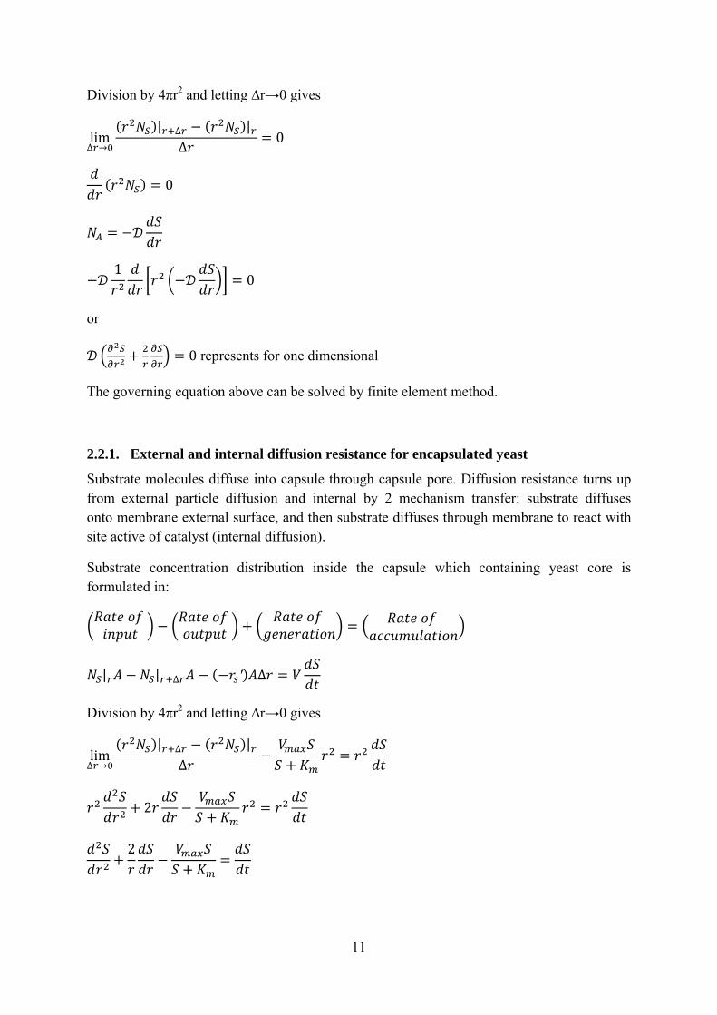
a. Discretize the continuum
Divide the solution region into non-overlapping elements or sub-regions. The finite
element discretization allows a variety of element shapes, for example, triangles,
quadrilaterals. There is an m element and an n node. Node is a point which separates 2
elements. For 1 dimensional partial differential have 2 nodes for each element.
Figure 2.Typical finite element mesh. Elements, nodes and edges.
b. Select interpolation or shape functions
It represents the variation of the field variable over an element.
c. Form element equations (Formulation)
The term "weak form" attributes to the partial differential equations (PDE) that are to be
solved. The solution of a boundary value problem described by a particular PDE can be
achieved by setting the PDE to a weak form. In general the solution of a PDE can be
14
performed from a "strong form" or from a "weak form". The strong form description of a
PDE is the one we have already known, for example the Laplace equation. Since the
finite element method is based on the discretization of the domain, the solution of the
strong form of the PDEs describing the problem must be descretized. For this purpose a
weak form is being developed. To develop a weak form of the equations, the integration
of the product of the trial functions with the equations must be performed. The trial (or
test) functions are assumed to be as smooth as possible so as they vanish on the
prescribed displacement boundary.
The term weak form is referred as variational form, because the solution of the PDEs is
approximated with the use of trial functions. The Galerkin method is one of the methods
that are based on the variational form of the equations. the variational formulation of a
physical problem is often referred to as the weak formulation.
After briefly describing the various elements used in the context of finite element
analysis, we shall now focus our attention on determining the element characteristics,
that is, the relation between the nodal unknowns and the corresponding loads or forces in
the form of the following matrix equation, namely,
K T ={f}
where [K] is the thermal stiffness matrix, {T} is the vector of unknown temperatures and
{f} is the thermal load, or forcing vector.
Next, we have to determine the matrix equations that express the properties of the
individual elements by forming an element Left Hand Side (LHS) matrix and load
vector.
For example, a typical LHS matrix and a load vector can be written as
K e=1 -1-1 1
{f}e
where the subscript e represents an element; Q is the total heat transferred; k is the
thermal conductivity; l is the length of a one-dimensional linear element and i and j
represent the nodes forming an element. The unknowns are the temperature values on the
nodes.

15
Consider the two-dimensional linear triangular elements shown in Figure 3. Let us
assume the following elemental LHS matrix for the variable φ
For element 1,
…. (3.1)
And for element 2,
…. (3.2)
The elemental RHS vectors are the following: For element 1,
f1
C1C2C3
… 3.3
and for element 2,
f2
d1d2d3
… 3.4
Figure 3.A domain with two linear triangular elements
d. Assemble the element equations to obtain a system of simultaneous equations
To find the properties of the overall system, we must assemble all the individual element
equations, that is, to combine the matrix equations of each element in an appropriate way
16
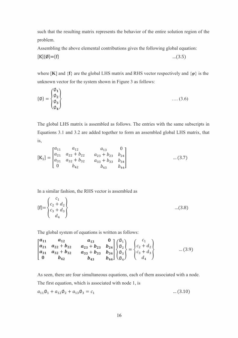
such that the resulting matrix represents the behavior of the entire solution region of the
problem.
Assembling the above elemental contributions gives the following global equation:
K Ø f … 3.5
where [K] and {f} are the global LHS matrix and RHS vector respectively and {φ} is the
unknown vector for the system shown in Figure 3 as follows:
…. (3.6)
The global LHS matrix is assembled as follows. The entries with the same subscripts in
Equations 3.1 and 3.2 are added together to form an assembled global LHS matrix, that
is,
K1
0
0
… 3.7
In a similar fashion, the RHS vector is assembled as
f … 3.8
The global system of equations is written as follows:
… 3.9
As seen, there are four simultaneous equations, each of them associated with a node.
The first equation, which is associated with node 1, is
… 3.10
17
In the above equation, the contributions are from node 1 and the nodes connected to node
1. As seen, node 1 receives contributions from 2 and 3. Similarly, the second nodal
equation receives contributions from all other nodes, which is obvious from Equation
3.9.
e. Solve the system of equations
The resulting set of algebraic equations
f. Calculate the secondary quantities
From the nodal values of the field variable, for example, temperatures can be calculated
the secondary quantities, for example, space heat fluxes.
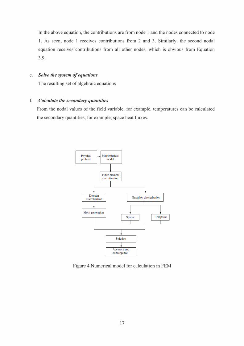
Figure 4.Numerical model for calculation in FEM

18
3.1.1. Two Dimensional Mass Flows
FE method is a numerical method to solve arbitrary differential equation. To achieve this
objective, it is a characteristic feature of the FE approach that the differential equations are
reformulated into an equivalent form, that so called weak formulation.
Weak form for is derived from strong form. The key point is the fundamental divergence
theorem of Gauss.
Strong form is considered in two-dimensional body and assumed that N is the amount mass
accumulated in the body per unit volume and per unit time, C the concentration, D the
constitutive matrix, and t the thickness. The flux vector k is determined from Fick’s law, i.e.
Q=-D C
d d … (3.11)
Where t=t(x,y) denotes the thickness in the z-direction of the body located in the xy-plane.
See below
Figure 5.Two-dimensional body with thickness t located in the xy-plane
We have that kn = kTn. Gauss’ divergence theorem yields:
d d d div d … (3.12)
With (3.11), (3.12) takes the form
div d 0 … (3.13)

19
div … (3.14)
which is the balance principle for the two-dimensional body. If the thickness is constant, we
get
div k = N … (3.15)
Using the constitutive equation in balance equation (3.14), it follows that
div 0 in region A … (3.16)
where region A is the entire region of the body. If the constitutive equation D is given by
(3.17)
00 ;
0 00 00 0
... (3.17)
For isotropic material, we obtain
0 … (3.18)
To solve the differential equation (3.16), boundary conditions are required. These boundaries
are typically of the form
C= g on Lg … (3.19)
where h and g are known quantities. Lh is that part of the boundary L on which the flux qn is
known, whereas Lg is that part of the boundary L on which the concentration C is known .
The sum of boundaries Lh and Lg constitutes the entire boundary L.
20
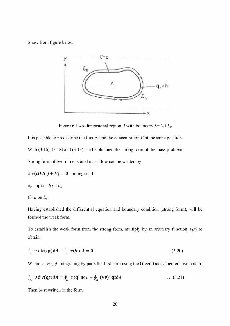
Show from figure below
Figure 6.Two-dimensional region A with boundary L=Lh+Lg
It is possible to prediscribe the flux qn and the concentration C at the same position.
With (3.16), (3.18) and (3.19) can be obtained the strong form of the mass problem:
Strong form of two-dimensional mass flow can be written by:
div 0 in region A
qn = qTn = h on Lh
C=q on Lg
Having established the differential equation and boundary condition (strong form), will be
formed the weak form.
To establish the weak form from the strong form, multiply by an arbitrary function, v(x) to
obtain:
div d d 0 ... (3.20)
Where v=v(x,y). Integrating by parts the first term using the Green-Gauss theorem, we obtain:
div d d … (3.21)
Then be rewritten in the form:
C=g
21
d d d ... (3.22)
We may use the boundary condition to obtain
d d d d … (3.23)
Where h is a known quality along Lh, whereas the flux qn is unknown along the boundary Lg.
Inserting the constitutive relation provides the following weak form:
d d d d … (3.24)
… (3.25)
where,
= arbitrary weight function
D = constitutive matrix
T = temperature
t = thickness
Q = mass flow per unit time per unit volume of the body
q = flux vector (Fick’s low)
From figure 6, the temperature is approximated in:
T = Na … (3.26)
Where N is global shape function matrix and a contains the temperature at the nodal points in
the entire body. This means that
N … ; a … (3.27)
where n is the number of nodal points for the entire body and a component N, depends on x
and y, i.e. Ni = Ni (x,y). From (3.26) we obtain
22
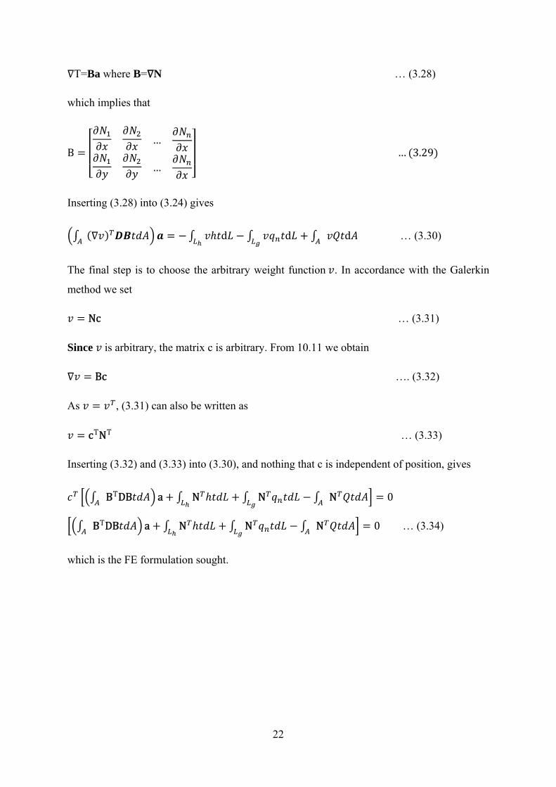
T=Ba where B= N … (3.28)
which implies that
B…
… … 3.29
Inserting (3.28) into (3.24) gives
d d d … (3.30)
The final step is to choose the arbitrary weight function . In accordance with the Galerkin
method we set
Nc … (3.31)
Since is arbitrary, the matrix c is arbitrary. From 10.11 we obtain
Bc …. (3.32)
As , (3.31) can also be written as
cTNT … (3.33)
Inserting (3.32) and (3.33) into (3.30), and nothing that c is independent of position, gives
BTDB a N N N 0
BTDB a N N N 0 … (3.34)
which is the FE formulation sought.

23
To write (3.34) in a more compact fashion, we define the following matrices:
K BTDB d
fb N h d N d
f1 NT d
As D has the dimension 2 x 2 and B the dimension 2 x n, it follows that K is a square matrix
with dimension n x n and it is the stiffness matrix. Likewise, both fb and fl have the dimension
n x 1 and they are termed the boundary vector and load vector, respectively.
Ka= fb + fl … (3.36)
We define the force vector f by
f= fb + f1 … (3.37)
(3.36) becomes
Ka = f … (3.38)
Region A with thickness t, the balance principle states that
… 3.39
f= fb + f1, i = 1,…,n …(3.40)
… 3.41
According to (3.35) we have that
d d … (3.42)
… (3.35)

24
We recall that the boundary condition specify the flux qn=h along Lh whereas the flux qn
along Lg is unspecified beforehand. Therefore, (3.42) may be written as
… (3.43)
From (3.35) a component of the load vector is given by
… (3.44)
Using (3.42) and (3.43) leads to
d d
d d … 3.45
A comparison with (3.39) shows that
0
This means that the balance principle for the body is expressed by the fact that the sum of the
components of the force vector f is equal to zero. We emphasize that (3.45) holds exactly
even though the finite element method is an approximate approach.
A
C = Na K
global
formulation

25
3.2.1. Convergence and Order Mesh Quality
The FE method provides an approximate solution to the problem at hand and it is obvious
that the more elements we use the more accurate the approximate solution. In the limit, when
the elements are infinitely small, we require that our approximate solution is infinitely close
to the exact solution. This is the convergence requirement [19].
The first step in an FE analysis is to select the type of elements and corresponding FE mesh.
There are no fixed rules on how to make these decisions. Clearly, for a given type of element
the accuracy increases with decreasing element size and, in general, one will use small
elements in regions where the unknown function- the concentration-varies rapidly[19].
Figure 7. a) Quadrilateral; b) Interior division; c) Desirable division
Figure 8.Mesh refinement
In order obtain an efficient solution scheme, we want to use few elements in regions where
the unknown function varies slowly, but many elements in regions where it varies rapidly.
Two possibilities, which allow for such a mesh refinement and which fulfill the continuity
requirement, are illustrated in fig. 8 for the three-node triangular element and four-node
rectangle.

26
It is obvious that the division in fig. 7(c) is better than that of 7(b), since the largest
dimension of the elements in 7(c) is smaller than that given by 7(b). The ratio between the
largest and the smallest dimension of an element is called the aspect ratio and in a good FE
mesh, the aspect ratio is as close as possible to unity.
The convergence order is a measure for the improvement of the solution as a consequence of
mesh refinement. In order to determine the convergence order from numerical runs, the errors
of runs with different refinement level have to be related.
The convergence of a numerical solution of one or several partial differential equations
generally depends on various characteristics of the problem, on the numerical algorithm, on
the mesh refinement and on the mesh quality. Solving the same problem with finer grid and
seeing the variation in result is a good way to analyze grid independence.

27
3.2. Simulation in Comsol Multiphysics
The diffusion module of Comsol Multiphysics was used to solve the encapsulated cell
problem. There are some step for modeling and simulating in Comsol.
Figure 9.Steps in Comsol simulation
Define 2D Geometry for half circle (on axis symmetry)
PDE Definition
- Choose Chemical Reaction Engineering- Diffusion as PDE
- Define parameter values within each subdomain (membrane, liquid core, and cell pellet)
- Define boundary conditions for axis symmetry, continuity and flux
Discretization
- Membrane and liquid core : automatic mesh - Cell pellet : maximum mesh element size is 5e-5 m
PDE Solution
Transient (time dependent) Choose FE solution algorithm
Post-Processing
Visualizations: surface plot Boundary integration : flux of glucose
28
3.2.1. Geometry and Mesh
This model introduces the concept of effective diffusivity in yeast encapsulated in spherical
porous membrane. Glucose passed through the membrane into capsule by diffusion. Capsule
was divided into three sections, which were membrane, liquid core and cell pellet. Capsule
had ca. 3.5 mm of diameter and 0.17 mm of thickness.
A simple geometry with a sphere was modeled to develop a model with acceptable results.
The aim was to decide which solver parameters and boundary conditions to use. The model
may not be exact like reality due to those assumptions. Inhibitor effects were not taken into
consideration.
Meshing was in free mesh parameters by including maximum element size. Free mesh
parameters can specify local mesh-element sizes and control the element distribution. Mesh
must be prescribed until we have grid independence and reach convergence. The case was set
up in 2D only. A symmetry axis was used to make the simulation run faster.
Comsol was used as software to create geometry and mesh, see figure 8The mesh in regions
of specific interest was adjusted. The interesting region was the pellet region in which the
mesh looked finer than in the others 2 subdomains. Maximum element size in membrane and
liquid core was set equal to the initial, and maximum size in cell pellet was 5e-5 m. The mesh
had to be irregular for it to be possible to generate a mesh. It was examined in Comsol if there
were any cells with high level of skewness. The number of cell in the mesh with no cell was
281 elements, with 25%-cell pellet was 1720 elements, with 50%-cell pellet was 3337
elements, with 75%-cell pellet was 5010 elements and in the mesh without liquid core was
6155 elements.

29
(a) (b) (c) (d) (e)
Figure 10.Mesh with no cell, 25%, 50%, 75%, and 100% of cell-filling
The artificial porous structure used in this model is depicted in Figure 11 below.
Figure 11.Artificial porous structure
Figure 11 shows the three subdomains. Membrane subdomain is CO4, liquid core is CO3,
and cell pellet is CO2.
Flux boundaries
Axis symmetry boundaries
Continuity boundaries
30
3.2.2. Model Definition and settings
The process that was simulated was the change in the concentration profiles in a capsule
which occurs when encapsulated cells react with glucose when the capsule is dipped into a
well-stirred glucose solution. Glucose passes through membrane and reacts in cell section.
The model equation in the modeled domains shown in Figure 11 is the time-dependent
equation
. (3.2.2.a)
where Cs denotes concentration (mol/m3 using SI units), D the diffusion coefficient (m2/s) of
the solute and R the reaction rate (mol/m3.s).
Reaction rate is Monod equation,
. . (3.2.2.b)
The boundary conditions are of 3 different types. A flux boundary condition applies at
capsule surface boundary in Figure 11. It is expressed as
. ; (3.2.2.c)
where n is the normal vector to the boundary, C is a concentration in every step. In the
equation for the flux condition, N0 is an arbitrary user-specified flux expression. In this case,
N0 was set to 0. Furthermore, kc represents the mass transfer coefficient and cb is the bulk
concentration in the fictitious diffusion layer at the boundary.
The conditions at the inner boundaries in Figure 11 were set as continuity, according to
. 0; (3.2.2.d)
This is the default boundary condition on interior boundaries and pair boundaries; it is not
applicable to exterior boundaries. The vertical boundary was considered to have axial
symmetry, according to
. 0 (3.2.2.e)
31
The axial symmetry condition is identical to the insulation/ symmetry condition. However,
the axial symmetry allows generation of 3D simulation by rotation.
As described above about model equation, diffusion and reaction model is straightforward to
solve this problem. Diffusion was approximated by constant diffusion coefficients of
substrate in the surface membrane, liquid core and cell pellet, respectively. Reaction was
approximated by Monod equation.
Diffusion and reaction equation was calculated from properties in Table 1.
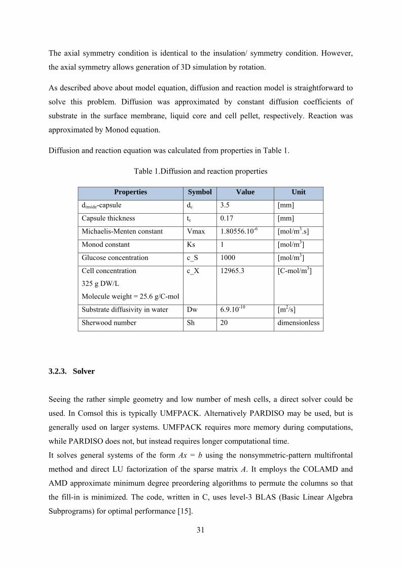
Table 1.Diffusion and reaction properties
Properties Symbol Value Unit
dinside-capsule dc 3.5 [mm]
Capsule thickness tc 0.17 [mm]
Michaelis-Menten constant Vmax 1.80556.10-6 [mol/m3.s]
Monod constant Ks 1 [mol/m3]
Glucose concentration c_S 1000 [mol/m3]
Cell concentration
325 g DW/L
Molecule weight = 25.6 g/C-mol
c_X 12965.3 [C-mol/m3]
Substrate diffusivity in water Dw 6.9.10-10 [m2/s]
Sherwood number Sh 20 dimensionless
3.2.3. Solver
Seeing the rather simple geometry and low number of mesh cells, a direct solver could be
used. In Comsol this is typically UMFPACK. Alternatively PARDISO may be used, but is
generally used on larger systems. UMFPACK requires more memory during computations,
while PARDISO does not, but instead requires longer computational time.
It solves general systems of the form Ax = b using the nonsymmetric-pattern multifrontal
method and direct LU factorization of the sparse matrix A. It employs the COLAMD and
AMD approximate minimum degree preordering algorithms to permute the columns so that
the fill-in is minimized. The code, written in C, uses level-3 BLAS (Basic Linear Algebra
Subprograms) for optimal performance [15].
32
4. RESULT AND DISCUSSION
4.1. Variation of diffusivities
Dm 90% Dw 50% Dw 10% Dw 1% Dw 0.1% Dw Scale
90% Dw 1
2
3
4
*
5
*
t = 320 min -rs= 4.44.10-5
t = 290 min -rs= 4.44.10-5
t = 990 min -rs= 4.44.10-5
t = 3333 min -rs= 4.45.10-5
t = 2433 min -rs= 1.48.10-5
50% Dw 6
7
8
9
*
10
*
t = 340 min -rs= 4.44.10-5
t = 470 min -rs= 4.44.10-5
t = 1000 min -rs= 4.44.10-5
t = 7833 min -rs= 4.44.10-5
t = 2450 min -rs= 1.48.10-5
10% Dw 11
12
13
14
*
15
*
t = 1120 min -rs= 4.44.10-5
t = 980 min -rs= 4.44.10-5
t = 1280 min -rs= 4.44.10-5
t = 8150 min -rs= 4.44.10-5
t = 2433 min -rs= 1.48.10-5
1% Dw 16
17
18
19
*
20
*
t = 1440 min -rs= 4.48.10-5
t = 1440 min -rs= 4.47.10-5
t = 1370 min -rs= 4.5.10-5
t = 8167 min -rs= 4.34.10-5
t = 2433 min -rs= 1.48.10-5
0.1%Dw 21
22
23
24
*
25
**
t = 1430 min -rs= 2.38.10-5
t = 1410 min -rs= 2.38.10-5
t = 1440 min -rs= 2.36.10-5
t = 8250 min -rs= 2.21.10-5
t = 2433 min -rs= 1.48.10-5
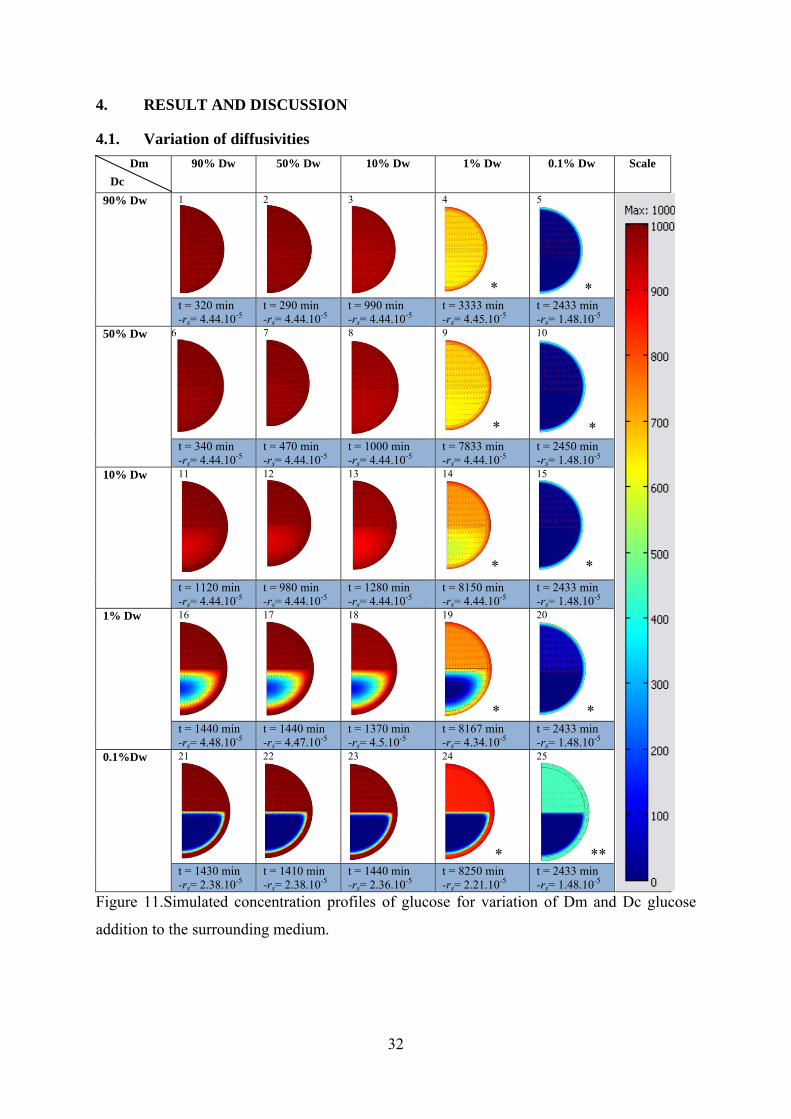
Figure 11.Simulated concentration profiles of glucose for variation of Dm and Dc glucose
addition to the surrounding medium.
Dc
33
Design 14 and 18 in Figure 11 had close to maximum overall reaction rate, but the
concentration profiles looked quite different, and it took longer time for design 14 to reach
steady state. Since it takes some time before glucose can diffuse into the center of the core, it
is likely that there are zones of low glucose concentration when the glucose is first added. To
investigate this, the concentration profiles at 1, 2 and 6 h were calculated (Figure 13).
Dw, Dm and Dc are the diffusivities in water, membrane and cell pellet, respectively; t: time
to reach steady state concentration profile; rs: integrated glucose flux across the membrane at
steady state. As an exception, the capsule which has one star icon means that the capsule
needs the long time to reach steady-state and two stars icon means that steady-state could not
be reached within 24 h.
In Figure 12, the glucose concentration profiles after 24 h at 50% cell pellet filling are shown
depending on various combinations of diffusivities in the capsule membrane and in the cell
pellet.
At high Dc (90% of Dw, 50%-Dw, 10%-Dw), the inside of the capsule still had a high
concentration of glucose, shown in red in the surface plot. This means that diffusion was
rapid enough to compensate for all glucose consumption, and the glucose consumption rate
was at its maximum in the whole cell pellet.
At small Dc (1% and 0.1%-Dw), there was a concentration gradient of glucose, as indicated
by changing in the color plot. The small Dc caused more visible changes in the concentration
within the capsule.
On the other hand, small value of Dc means that it took a long time for the glucose to reach
the cell pellet, to react. The time, needed to reach a steady-state concentration profile was
over 24 hours.
Change of Dm did not cause any significant change to the concentration gradient, only to the
overall concentration level. This indicates that diffusivities in the cell pellet-Dc were rather
more important than the diffusivity of the membrane capsule.
34
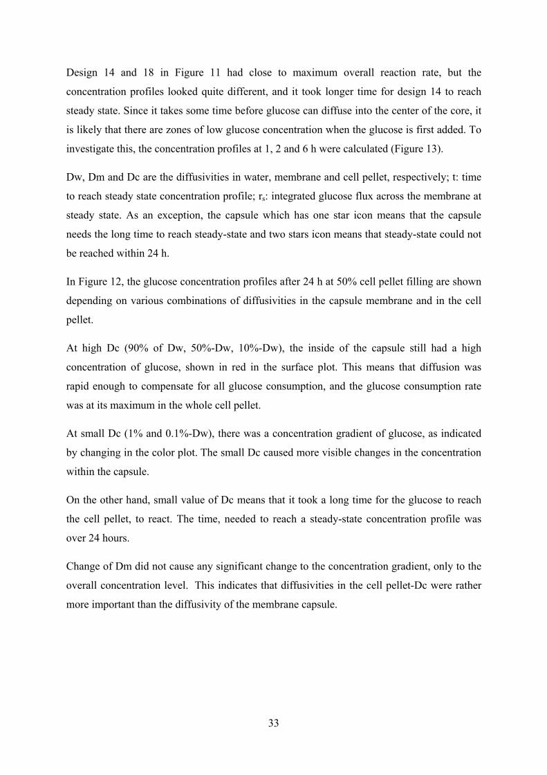
The relationship between rate (-rs) and glucose concentration is that the glucose concentration
must be very low before the rate actually decreases. If S=20*Ks then r=20/21*Vmax and if
S=5*Ks then r=5/6*Vmax. The scale for 0-5 mmol/L and 0-20 mmol/L can be shown below.
Design with low membrane diffusivities Scale
19 20 21 22
23 24 25
Figure 12.Diffusion limitation of Design 19-25 at concentration of glucose < 20 mol/m3.
Glucose limitation was defined as S<5*KS, corresponding to V<83% of Vmax.
At figure 11, the maximum overall reaction rate on design 14 and 18 is almost similar. Both
glucose concentration profiles and the time to reach steady-state are quite different. It can be
assumed that there are zones where the glucose diffuses into the center of core very slowly at
the first added. This case can be investigated by looking at concentration profiles during 1, 2
and 6 first hour.

35
1 hours 2 hours 6 hours Scale
Design 14
Design 18
Design 14
Design 18
Figure 13.Concentration profile of glucose at different time of cultivation.
Design 14 with Dm = 6.9e-12 and Dc = 6.9e-11 had a zone with lower than 5 mol/m3 of
glucose concentration at 1 hours cultivation. There was still a zone below 20 mol/m3 of
glucose at 2 hours cultivation.
Design 18 with Dm = 6.9e-11 and Dc = 6.9e-12 had larger zones below 5 mol/m3 of glucose
at 1 hours cultivation and below 20 mol/m3 of glucose at 2 hours cultivation.
Despite the lower Dm, concentration of glucose at Dc= 6.9e-11 (design 14) is higher than
concentration at Dc= 6.9e-12 (design 18). At Dc= 6.9e-12 only little glucose was available
within the cell pellet during the first hours.
36
Diffusion limitation can be analyzed from this part. Thus, at Dc= 6.9e-11 or lower, diffusion
limitation leads to glucose limitation during the first few hours of cultivation.
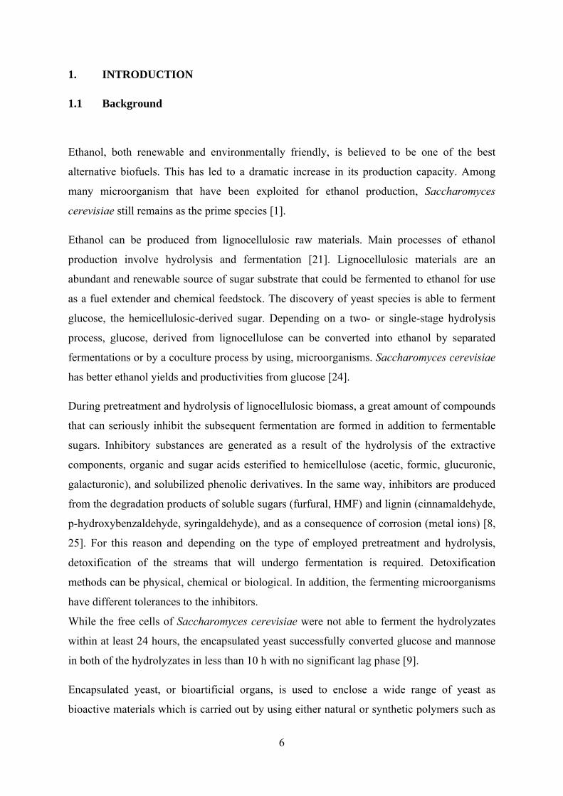
4.2. Variation of Cell-filling
The glucose concentration profile not only depend on the diffusion of the glucose but also on
the size of the cell pellet, since this will both affect the rate of reaction and the diffusion
distances. Therefore, the concentration profiles at different degrees of cell filling were
calculated at two combinations of membrane and cell pellet diffusivities.
Diffusivity 25%-cell filling 50%-cell filling 75%-cell filling 100%-cell filling Scale
Dm = 1% Dw
Dc = 10% Dw
t = 1667 min -rs= 2.00.10-5
t = 8150 min -rs= 4.43.10-5
t = 8167 min -rs= 7.50.10-5
t = 5000 min -rs= 8.88.10-5
Dm = 10% Dw
Dc = 1% Dw
t = 1663 min -rs= 1.39.10-5
t = 1370 min -rs= 4.50.10-5
t = 7667 min -rs= 7.07.10-5
t = 4933 min -rs= 8.88.10-5
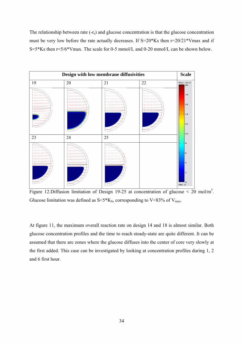
Figure 14.Concentration profile of different cell-filling at 24 hours cultivation
In these two combinations, the overall reaction rate is higher the more cells are in the capsule.
Nevertheless, there were low levels in the center of the larger cell pellets. Reaction rate is
higher with increasing cell filling. At 50%-cell filling concentration profile, gradient
concentration seems to be more stable than others. The smallest cell filling has higher glucose
concentration in cell pellet whereas the biggest cell filling has lower glucose concentration in
cell pellet.

37
At 50% cell-filling shows more stable concentration profile. I can be assumed that cell and
the glucose has a more convenience space to react each other.
It is interesting to look at the concentration profile for several cell-filling at 1, 2 and 6 h to
investigate how glucose concentration depends on its diffusion into center core.
The glucose concentration can be investigated by looking at 1, 2 and 6 h after glucoses added.
Glucose
Limitation
Filling 1 hours 2 hours 6 hours Scale
5 mmol/L 50%
75%
100%
Figure 15a.Concentration profile of glucose for different cell-filling at different time of
cultivation for Dm = 1% Dw; Dc = 10% Dw and scaling for 0-5 mmol/L

38
Glucose
Limitation
Filling 1 hours 2 hours 6 hours Scale
20 mmol/L 50%
75%
100%
Figure 15b.Concentration profile of glucose for different cell-filling at different time of
cultivation for Dm = 1% Dw; Dc = 10% Dw and scaling for 0-20 mmol/L
Diffusion limitation for scale 0-5 mmol/L and 0-20 mmol/L are showed in 50-100% cell-
filling during 1 and 2 hour at the first glucose added.
It means that at this time, the rate decreases after the glucose concentration in the 5 and 20 mmol/L.
In cultivations performed by Talebnia, glucose was converted within 10 h without significant
lag phase [7]. Due to the diffusivity in cell pellet gives the diffusion limitation during the
cultivation.

39
Glucose
Limitation
Filling 1 hours 2 hours 6 hours Scale
5 25%
50%
75%
100%
Figure 15c.Concentration profile of glucose for different cell-filling at different time of
cultivation (Dm = 10% Dw; Dc = 1% Dw), scaling for 0-5 mmol/L

40
Glucose
Limitation
Filling 1 hours 2 hours 6 hours Scale
20 25%
50%
75%
100%
Figure 15d.Concentration profile of glucose for different cell-filling at different time of
cultivation (Dm = 10% Dw; Dc = 1% Dw), scaling for 0-20 mmol/L

41
For 25%-cell filling, Figure 15 shows low rate of glucose consumption, but it took short time
to reach steady-state condition. At higher cell-filling, longer time was needed to reach steady-
state condition but the final rate of glucose consumption was higher, despite the large
diffusion limited zones.
5. Conclusions
There are several things to conclude for this case, that is:
a. A framework for simulating concentration profiles in yeast capsules has been created.
Comsol can solve this case by chemical reaction engineering multiphysics. It is difficult
to validate exact value within the capsule. The solver is in qualitative result properly,
which shows from surface plot (concentration profile).
b. By making combination of Dm and Dc value gives the effect for rate limiting
concentration during a few hours after glucose addition. The longer time to rech steady
state is needed when the cell pellet was <1%.
c. The diffusion phenomena of glucose through the capsule are influenced by external and
internal diffusion. The external diffusion which represent from membrane of capsule
doesn’t affect the rates very much. In the other hand, the internal diffusion, specifically
for cell diffusivity affects the rate very much. A 50% of cell-filling is more stable of
concentration profile than other, it can also be caused by electrostatic, hydrophobic or
hydrophilic from substrate and capsule.
6. Future Outlook
This work is still very simple, for modeling and simulation. For future work I suggest:
a. Include inhibitor effects in the reaction kinetics.
b. Keep working in Comsol for simulation by including cell growth
c. Look for ways of validating concentration profiles with experimental studies
d. Make a complete simulation to CFD for greater system. Look at CFD effect of glucose
transportation pass through into encapsulated yeast during the cultivation in continuous
stirrer tank reactor by turbulence assumption

42
REFERENCES
1. Bai, F. W., et al.,. Ethanol Fermentation technologies from sugar and starch feedstock.
Biotechnology Advanced 26: 89-105, 2008
2. Azhar, A.F., Bery, M. K., Colcord, A. R., Roberts, R. S., and Corbitt, G. V.:
Factors affecting alcohol fermentation of wood acid hydrolyzate. Biotechnol. Bioeng.
Symp., 11: 293-300 , 1981.
3. Cbung, I. S. and Lee, Y. Y.: Ethanol Fermentation of Crude Acid Hyrolyzate of
Cellulose Using High-Level Yeast Inocula. 2nd edition. Academic Press, San
Diego,1993.
4. A. Martinez, M.E. Rodriguez, M.L. Wells, S.W. York, J.F. Preston and
L.O.Ingram, Detoxification of dilute acid hydrolysates of lignocellulose with lime,
Biotechnol Progr 17, p. 287–293,2001
5. Talebnia, F and M.J. Taherzadeh. In situ detoxification and continuous cultivation of
dilute-acid hydrolyzate to ethanol by encapsulated S. cerevisiae, J Biotechnol 125, p.
377–384, 2006.
6. Licht, F.O. 2006. World Ethanol Market: The Outlook to 2015, Tunbridge Wells, Agra
Europe Special Report, UK.
7. Talebnia, F. Ethanol Production from Cellulosic Biomass by Encapsulated
Saccharomyces cereviseae.Chalmers University of Technology, Dep. of Chemical and
Biological Engineering,2008..
8. Palmqvist, E., Hahn-Hagerdal, B., 2000b. Fermentation of lignocellulosic hydrolysates.
II: inhibitors and mechanisms of inhibition. Bioresource Technology 74: 25–33..
9. Talebnia, F., Niklasson, C., and Taherzadeh, M.J., 2005. Ethanol Production From
Glucose and Dilute-Acid Hydrolyzates by Encapsulated S. cereviseae. Biotechnol
Bioeng 90(3):345-53.

43
10. Nielsen, J,Bioreaction engineering principles.—2nd ed/ Jens Nielsen, John Villadsen
and Gunnar Liden. ISBN 0-306-47349-6, 2002.
11. Chung and Lee, 1985. I.S. Chung and Y.Y. Lee , Ethanol production of crude acid
hydrolysate of cellulose using high level yeast inocula. Biotechnol.
Bioengng. 27 (1985), pp. 308–315
11. Fogler, H. Scott. Elements of Chemical Reaction Engineering. u.o : Pearson
Education, 2006, 4th edition.
12. Matthias K. Gobbert . Alginate as immobilization matrix for cells. TIBTECH-
MARCH 1990. Vol. 8, p.75-76. 2001-2008.
13. Anderson, Bengt, Ronnie Andresson, Love Håkansson, Mikael Mortensen,
Rahman Sudiyo, Berend van Wachem. Computational Fluid Dynamics for Chemical
Engineers. Gotheburg: u. n., 2008.
14. Talebnia, F., C., Taherzadeh, M.J. (2007): Physiological and Morphological Study of
Encapsulated Saccharomyces cerevisiae, Enzyme Microb. Technol., 41(6-7): 683-688
15. Comsol AB. Comsol Multiphysics 3.5a Documentation. 2008
16. Koyama, K and Minoru, S. Keitaoroevaluation of mass-transfer characteristics in
alginate-membrane liquid-core capsules prepared using Polyethylene Glycol,
98(2):p.114, 2004.
17. Cheong SH, Park JK, Kim BS, Chang HN. 1993. Microencapsulation of yeast cells in
calcium alginate membrane. Biotechnol Tech 7: 879-884.
18. Tanaka, H., Matsumura, M., and Veliky, I. A., Diffusion characteristic of substrate
in Ca-alginate gel beads. Biotechnology and Bioengineering, 26(1): p 53-58, 2004.
19. Ottosen, N and Peters on, H., Introduction to finite element methods. Pearson Prentice
Hall. 1992;p.81-85,91223
20. Hamdi, M. Biofilm thickness effect on the iffusion limitation in the bioprocess
reaction: Biofloc critical diameter significance. Bioprocess engineering,p. 193, 1995.
21. Wijayanti, Sri, Evaluation of an Alginate-Chitosan-Microcrystalline Cellulose Sulfate
Macroencapsulation System for Efficient Fermentation of Lignocellulosic Hydrolyzate ,
Master of Science Thesis in Industrial Biotechnology, Chalmers, 2009.

44
22. Chang, H. N., et al., 1996. Microencapsulation of recombinant Saccharomyces
cerevisiae cells with invertase activity in liquid-corenalginate capsules. Biotechnology
and Bioengineering 51: 157-162.
23. Park, J. K., and Chang, H. N., 2000. Fermentation of lignocellulosic hydrolysates for
ethanol production. Enzyme and Microbial Technology 18: 312-331.
24. Delgenes J.P. Moletta R.; Navarro J.M., 1996. Effects of lignocellulose degradation
products on ethanol fermentations of glucose and xylose by Saccharomyces cerevisiae,
Zymomonas mobilis, Pichia stipitis, and Candida shehatae. Enzyme and Microbial
Technology 19 : 220-225
25. Lynd, L.R., 1996. Overview and evaluation of fuel ethanol from cellulosic biomass:
technology, Economics, the Environment, and Policy. Annual Review of Energy and the
Environment 21: 403–465.
26. Orive, G., et al., 2004. Histrory, challenges and perpectives of cell microencapsulation.
Trends in Biotechnology 22: 87-92.
27. Bhatia, S. R., et al., 2005. Polyelectrolytes for cell encapsulation. Current Opinion in
Colloid & Interface Science 10: 45-51.
28. Chung. 1972. Effects of Local Applications of Microencapsulated Catalase on the
Response of Oral Lesions to Hydrogen Peroxide in Acatalasemia. Journal of Dental
Reserch: 319-321
29. Lim, F. and Sun, A.M., Microencapsulated islets as bioartificial endocrine pancreas.
Science, 210 (1980) 908-910.
30. Lewis, R. W. and Perumal, N. Fundamentals of the Finite Element Method for Heat and
Fluid Flow. Wiley.
Recommended