Munich Personal RePEc Archive
Modal composition of cargo
transportation and income inequality in
Brazil
Azzoni, Carlos Roberto and Guilhoto, Joaquim M.
2008
Online at https://mpra.ub.uni-muenchen.de/31411/
MPRA Paper No. 31411, posted 10 Jun 2011 16:51 UTC

1
Modal Composition of Cargo Transportation
and Income Inequality in Brazil
Carlos R. Azzoni1
Joaquim M. Guilhoto2
Abstract
A Leontief-Miyazawa model was estimated to measure the income distribution
effects of changes in the modal composition of cargo transportation in Brazil. It was
calibrated for year of 2004, and considers 31 sectors (4 of which are related to cargo
transportation: road, rail, water, and air), and 10 income brackets. A transfer of 10% of
road transportation to rail or water was simulated. The results show that the relative
impacts are small, considering the size of the Brazilian economy and the small
importance of the transportation sector. Increases in the share of rail or water
transportation will increase GDP and personal income, but will decrease employment.
Increases in the share of rail transportation will have more positive effects on personal
income and income distribution than increases in the share of water transportation. A
change to water will result in a larger GDP change and a smaller number of jobs lost in
comparison to a change to rail. Although rail and water present larger shares of
intermediate purchases from pro-poor sectors than road transportation, the latter
distributes directly more income to the low income brackets. On balance, the result is a
very modest change in the Gini coefficient.
1 Department of Economics, FEA - University of São Paulo, Brazil; CNPq Scholar; E-mail: [email protected] 2 Department of Economics, FEA - University of São Paulo, Brazil; REAL, University of Illinois; and CNPq Scholar; E-mail: [email protected]

2
1. Introduction
Brazil is a large country with a complex and inefficient transportation system. It
is been argued that the problems related to this sector are at the nucleus of the so called
“Brazil Cost”. The process of growth generates an increasing demand of transportation
of products and raw materials. Any weakness of the transportation system restricts the
development not because it restricts gain possibilities through commerce, but also
because a poor infrastructure can affect adversely the productivity growth in other
sectors.
Table 1 and Figures 1 and 2 present the volume of Brazilian modal composition
of cargo transportation in 2004. It is clear that road dominates, with over 46% of
volume, followed by water and, in third place, rail. More than 60% of the load is
transported in highways. Water transportation is second in terms of volume but accounts
for only 14.2% of the total ton-km in the economy, while the share of the railroads is
21.6%.
Table 1 – Modal Composition of Cargo Transportation in Brazil, 2004
Mode Volume (ton) Ton-km of freight (million)
Road 665.578.033 46,5% 485.625 63.8%Rail 356.136.024 24,9% 164.809 21.6%Water 398.965.699 27,9% 108.000 14.2%Air 11.457.095 0,8% 3.169 0.4%Sum 1.432.136.851 100,0% 761.603 100.0%
Source: CNT.

3
Figure 1– Shares of Different Transportation Modes – Volume
46.47%
24.87%
27.86%
0.80%
Road
Railroad
Waterborne
Air
Source: CNT.
Figure 2 – Shares of Different Transportation Modes – Ton-Km of Freight
61.09%
20.73%
13.59%
4.19% 0.40%
Road
Railroad
Waterborne
Pipeline
Air
Source: CNT.
The Brazilian modal distribution of cargo transportation, excessively
concentrated in the highways system, which is showed in Figure 3, is the result of a
process of fast and disproportional enlargement of the road sector, relatively to the other
modes. In consequence, the road network is an important instrument to the greater
agility in the transportation of cargo and passengers, since the highways are

4
fundamental links in the modern production chains, in function of their great flexibility
and capability of answering fast to the demands – the highways, then, are relevant assets
that should be maintained and amplified.
Figure 3 – Highways in Brazil
Source: Caliper of Brazil.
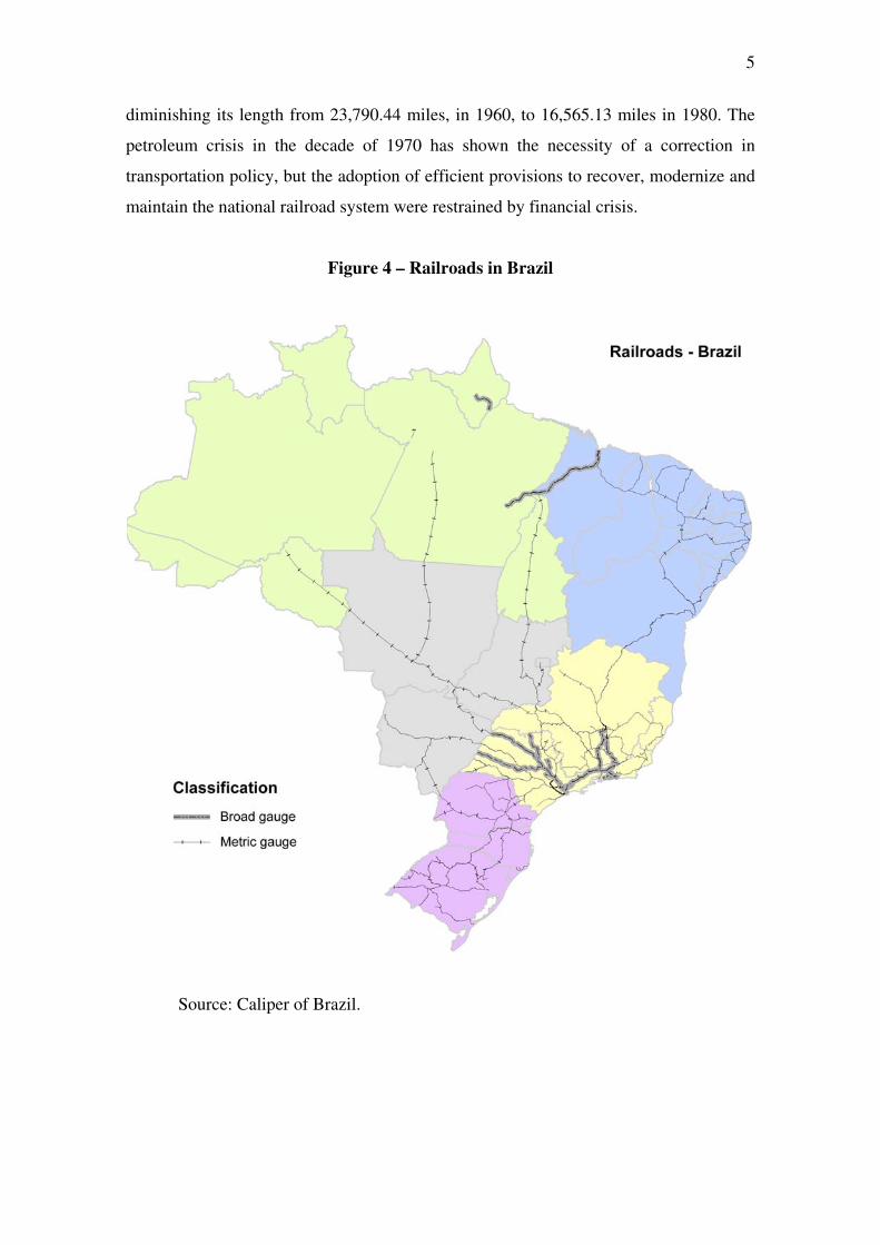
The actual railroad system, showed in Figure 4, has developed in an accelerated
way from 1854, when it was inaugurated the first railroad, to 1920. The decade of 1940
marks the beginning of the stagnation process, stressed with the central government
emphasis in the highway system. Many railroads and its branches were deactivated
5
diminishing its length from 23,790.44 miles, in 1960, to 16,565.13 miles in 1980. The
petroleum crisis in the decade of 1970 has shown the necessity of a correction in
transportation policy, but the adoption of efficient provisions to recover, modernize and
maintain the national railroad system were restrained by financial crisis.
Figure 4 – Railroads in Brazil
Source: Caliper of Brazil.
6
Any attempt to change the modal composition of cargo transportation will
require investments and will produce many consequences into the economic system. Of
special interest to this study is the impact of these possible changes on income
inequality in the country. For that, a Leontief-Miazawa type of model was estimated,
allowing for the estimation of the effects of changes in the participation modes of
transportation on the Gini coefficient, a national indicator of income inequality. The
next section presents the methodology, indicating how the impacts were measured.
Section 3 describes the data used in the study, indicating sources and presenting general
information on their main characteristics. The results of the estimation of the model are
presented and discussed in Section 4. The last section concludes the study.
2. Methodology
In order to analyze the impacts of changes in the modal composition of cargo
transportation in Brazil, a Leontief-Miazawa type of model will be estimated. The input-
output relationships are considered, but so are the sectoral distribution of income to
households in different income brackets, and the sectoral allocation of consumption
expenditures by households.
The Static Model
The intersectoral flows existing in a given economy, which are determined by
both technological and economic factors, can be described by a system of simultaneous
equations represented by
X AX Y= + (1)
where X is a (n x 1) vector with the total output of each sector, Y is a (n x 1) vector of
final demand for each sector, and A is a (n x n) matrix of technical coefficients of
production (Leontief, 1951). The sectoral final demands are usually treated as
exogenous to the system and, therefore, the output vector is uniquely determined given
the final demand vector, that is,

7
1( )X I A Y−= − (2)
where I is the (n x n) identity matrix and 1( )I A−− is the (n x n) Leontief inverse matrix.
The vector of final demands, however, is the sum of a vector of consumption
demands and a vector of exogenous demands (i.e., government expenditure, investment,
and exports):
ecYYY += (3)
where Y c is the (n x 1) vector of consumption demand and Y e is the(n x 1) vector of
exogenous demand.
Considering that consumption demand are related to income, in the tradition of
Keynes and Kalecki (see Miyazawa, 1960, 1963, and 1976, Keynes, 1936, e Kalecki,
1968 e 1971), the multisectoral consumption function is defined as
CQYc = (4)
where C is a (n x r) matrix with the consumption coefficients, and Q is a (r x 1) vector
with the total income of each income group.
Let E be a matrix whose elements eik represent the total amount of the ith
commodity consumed by the kth income group, and be defined as ik
c
k
ikik
q
ec = (5)
Since “(...) the consumption structure generally depends on the structure of
income distribution” (Miyazawa, 1976, p. 1), it is necessary to include the way income
is distributed by sector. The income-distribution structure can be represented by the
simultaneous equations
VXQ = (6)

8
where V is a (r x n) matrix with the value-added ratios. The simultaneous equations (6)
represent the fact that the productive structure prevailing in a country is associated to a
corresponding structure of income distribution.
Let R be a matrix whose elements represent the income of the kkj
rth group
earned from the jth sector. Then, v is given by kj
j
kj
kjx
rv = (7)
To solve static model we start by substituting (3), (4), and (6) into (1), getting
eYCVXAXX ++= (8)
whose solution is (9) ( eYCVAIX
1−−−= )Moreover, it is convenient to express the matrix in (9) as the product of
- which reflects the production flows - and another matrix reflecting the
endogenous consumption flows, that is,
( ) 1−−= AIB
( ) eYCVBIBX
1−−= (10)
Finally, substituting (10) into (6), the multisectoral income multiplier is given by
( ) 1 eQ VB I CVB Y
−= − (11)
which shows that the income for each group (and, of course, the aggregate income) will
have different values depending on the sectors' shares in the exogenous final demand
(Miyazawa, 1963 and 1976).

9
2.2. The Dynamic Model
The model derived in sub-section does not take into account time lags. To make
the model more realistic, one should account for the fact that changes in the sectoral
output levels do not cause changes in consumption (through changes in the different
income groups) immediately, but only after a certain period of time, that is,
1
c
kY CVX −=
k (12)
where k means a time period, and k-1 means the previous time period. Equation (8) then
becomes
1
e
k k kX AX CVX Y−= + + (13) or 1
e
k KX BCVX BY−− = (14)
which is a non-homogeneous system of first-order linear difference equations with
constant coefficients.
Given the one-period lag between production and consumption in (12), equation
(14) can be used to analyze the dynamic behavior of the model and, in particular, the
convergence of the system to the steady-state solution in (8). The solution of equation
(14) is given by the sum of the complementary solution - i. e., the solution of the
homogeneous system - and a particular solution - i. e., a solution for the complete
system (see Goldberg, 1958). The homogeneous version of (14) is
1 0k K
X BCVX −− = (15)
and its solution is given by
( )k
kX BCV G= (16)
where the (n x 1) vector G will be determined by the initial condition.
A particular solution can be found by making 1k kX X − X= = , i.e.,
10
eX BCVX BY− = (17)
The solution being
( ) 1 eX I BCV BY
−= − (18)
The final solution is then given by the sum of (16) and (18), i.e.,
( ) ( ) 1k e
kX BCV G I BCV BY−= + − (19)
Given the initial condition 0X , vector G can be found by solving the system for
, that is, 0k =
( ) 1
0
eG X I BCV BY
−= − − (20)
Moreover, the steady-state solution of the model is given by equation (18), and
is identical to the solution of the static model (equation 10)3.
By the theory of eigenvalues and eigenvectors (Strang 1980), matrix ( )kBCV
can be expressed as
( ) 1k kBCV S S
−= Λ (21)
3 The fact that equations (10) and (18) are identical can be seen by an algebraic manipulation of the
matrices in equation (8):
( ) ( )
( )
( )
11 1
11
11
1
B I BCV I CVB B
B CV
B I BCV
I BCV B
−− −
−−
−−
−
⎡ ⎤− = −⎣ ⎦
⎡ ⎤= −⎣ ⎦
⎡ ⎤= −⎣ ⎦
= −
11
where S is a (n x n) matrix whose columns (linearly independent by hypothesis) are
eigenvectors of , and is a (n x n) diagonal matrix with the eigenvalues of
.
(BCV ) Λ
( )BCV
Substituting (21) into the homogeneous solution (16) gives:
1k
kX S S G−= Λ (22)
As k approaches infinity, the system will converge to the steady-state solution
(18) if ( k)BCV goes to zero. The sufficient condition for the system to converge is that
the eigenvalues of ( , )BCViγ , must be in the interval 0 iγ 1≤ < , for all i.
3. Data description
The model described in Section 2 was applied to Brazilian data in order to assess
the impacts of changes in the modal composition of cargo transportation in the country
on income inequality. This section describes the data used.
The productive structure
A Social Accounting Matrix was assembled to take care of the task at hand. Its
central piece is the Input-Output table, referring to 2004. Given the recent modifications
in the calculation of National Accounts in Brazil4, the system used in Moreira et all.
(2007) was updated, applying the methodology presented in Guilhoto and Sesso-Filho
(2005). All productive activities of the economy were allocated to one of 35 sectors,
listed in Table 2. The transportation sector, which appears was an aggregate sector in
the National Accounts System, was disaggregated into four cargo sub-sectors: road, rail,
water, and air, and one for passenger transportation (highlighted in the Table). In order
to disaggregate the transportation sector, specific information sector was gathered from
4 http://www.ibge.gov.br/home/estatistica/economia/contasnacionais/referencia2000/2005/default.shtm

12
the 2004 PAS - Pesquisa Anual de Serviços (Annual Survey of Services), by IBGE5.
The final results are presented in the appendix.
Table 2 - List of Sectors of the I-O Table
1 Agriculture
2 Mineral extraction (except fuel)
3 Petrol and gas
4 Non-metallic minerals
5 Steel and Non-ferrous metallurgy6 Machinery and equipment
7 Electric material and electronic equipment
8 All types of vehicles
9 Wood and furniture
10 Cellulose, paper and printing
11 Rubber
12 Chemical
13 Petrol refining
14 Pharmaceutical and veterinary
15 Plastics
16 Textiles
17 Apparel18 Shoes
19 General food
20 Other manufacturing
21 Public utility services
22 Construction
23 Trade
24 Road Transportation
25 Rail Transportation
26 Water Transportation
27 Air Transportation
28 Passengers Transportation
29 Communication
30 Financial institutions31 Services to households
32 Services to business
33 Building Rent
34 Public administration
35 Non-business private services
5 http://www.ibge.gov.br/home/estatistica/economia/comercioeservico/pas/pas2004/default.shtm

13
Sectoral distribution of income
The source of income distribution data by sector is the PNAD – Pesquisa
Nacional por Amostra de Domicílios, a national survey on a sample of 389,354
individuals and 139,157 households implemented in 20046. The interviewers collected
information on different aspects of socio-economic conditions. Of special interest for
this study is the amount of income received and the sector of activity of each person.
With that we could associate persons to sectors and their respective income. We
considered the monthly income in the activity referring to the sector, excluding
retirement payments and domestic servants. For each sector we have the total income
distributed, which were allocated to ten income classes, presented in Table 3, which also
presents the proportion of income appropriated. The intervals are the ones used by
IBGE – Instituto Brasileiro de Geografia e Estatística, the official statistics office.
The numbers presented in the table are also plotted in Figure 5, in which the
cumulative percentage of total income is displayed in the vertical axes. For comparison
purposes, the income distribution profile for the aggregate of all sectors is displayed in
each graph, so that comparisons can be made. It can be seen that the transportation of
passengers follows a similar pattern to the average of all sectors in classes 1 and 2 and
presents less concentration there-on, which indicates that it is less conducive to income
concentration than the average. On the other extreme, air transportation presents less
cumulative income for all classes, meaning that it is a sector with more income
concentration than the average.
6 www.ibge.gov.br/
14
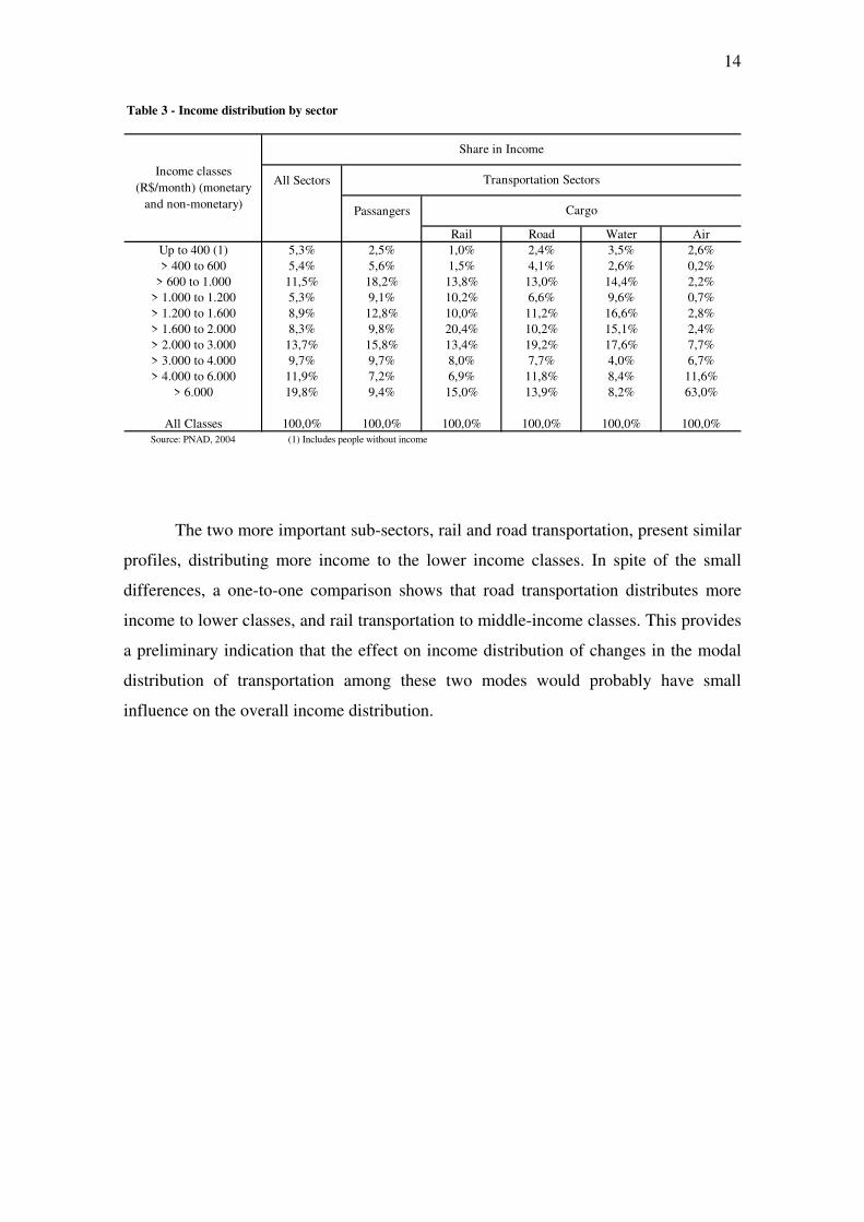
Table 3 - Income distribution by sector
All Sectors
Passangers
Rail Road Water Air
Up to 400 (1) 5,3% 2,5% 1,0% 2,4% 3,5% 2,6%
> 400 to 600 5,4% 5,6% 1,5% 4,1% 2,6% 0,2%
> 600 to 1.000 11,5% 18,2% 13,8% 13,0% 14,4% 2,2%
> 1.000 to 1.200 5,3% 9,1% 10,2% 6,6% 9,6% 0,7%
> 1.200 to 1.600 8,9% 12,8% 10,0% 11,2% 16,6% 2,8%
> 1.600 to 2.000 8,3% 9,8% 20,4% 10,2% 15,1% 2,4%
> 2.000 to 3.000 13,7% 15,8% 13,4% 19,2% 17,6% 7,7%
> 3.000 to 4.000 9,7% 9,7% 8,0% 7,7% 4,0% 6,7%
> 4.000 to 6.000 11,9% 7,2% 6,9% 11,8% 8,4% 11,6%
> 6.000 19,8% 9,4% 15,0% 13,9% 8,2% 63,0%
All Classes 100,0% 100,0% 100,0% 100,0% 100,0% 100,0% Source: PNAD, 2004 (1) Includes people without income
Income classes
(R$/month) (monetary
and non-monetary)
Share in Income
Transportation Sectors
Cargo
The two more important sub-sectors, rail and road transportation, present similar
profiles, distributing more income to the lower income classes. In spite of the small
differences, a one-to-one comparison shows that road transportation distributes more
income to lower classes, and rail transportation to middle-income classes. This provides
a preliminary indication that the effect on income distribution of changes in the modal
distribution of transportation among these two modes would probably have small
influence on the overall income distribution.

15
Figure 5 – Income distribution profiles within transportation sectors
Figure 4 - Income distrubution profiles within transportation sectors
0,0%
100,0%
Up to 400 (1) > 400 to 600 > 600 to 1.000 > 1.000 to 1.200 > 1.200 to 1.600 > 1.600 to 2.000 > 2.000 to 3.000 > 3.000 to 4.000 > 4.000 to 6.000 > 6.000
Cu
mu
lati
ve %
of
To
tal
Inco
me
All Sectors
Passengers
0,0%
100,0%
Up to 400 (1) > 400 to 600 > 600 to 1.000 > 1.000 to
1.200
> 1.200 to
1.600
> 1.600 to
2.000
> 2.000 to
3.000
> 3.000 to
4.000
> 4.000 to
6.000
> 6.000
Cu
mu
lati
ve %
of
To
tal
Inco
me
All Sectors
Water
0,0%
100,0%
Up to 400 (1) > 400 to 600 > 600 to 1.000 > 1.000 to 1.200 > 1.200 to 1.600 > 1.600 to 2.000 > 2.000 to 3.000 > 3.000 to 4.000 > 4.000 to 6.000 > 6.000
Cu
mu
lati
ve %
of
To
tal
Inco
me
All Sectors
Air
0,0%
100,0%
Up to 400 (1) > 400 to 600 > 600 to 1.000 > 1.000 to
1.200
> 1.200 to
1.600
> 1.600 to
2.000
> 2.000 to
3.000
> 3.000 to
4.000
> 4.000 to
6.000
> 6.000
Cu
mu
lati
ve
% o
f T
ota
l In
co
me
All Sectors
Rail
0,0%
100,0%
Up to 400 (1) > 400 to 600 > 600 to 1.000 > 1.000 to
1.200
> 1.200 to
1.600
> 1.600 to
2.000
> 2.000 to
3.000
> 3.000 to
4.000
> 4.000 to
6.000
> 6.000
Cu
mu
lati
ve %
of
To
tal
Inco
me
All Sectors
Road
Distributive profiles: road x train
0,0%
100,0%
Up to 400
(1)
> 400 to 600 > 600 to
1.000
> 1.000 to
1.200
> 1.200 to
1.600
> 1.600 to
2.000
> 2.000 to
3.000
> 3.000 to
4.000
> 4.000 to
6.000
> 6.000
Cu
mu
lati
ve
% o
f T
ota
l In
co
me
Rail
Source: Research data
Road
16
Employment by sector
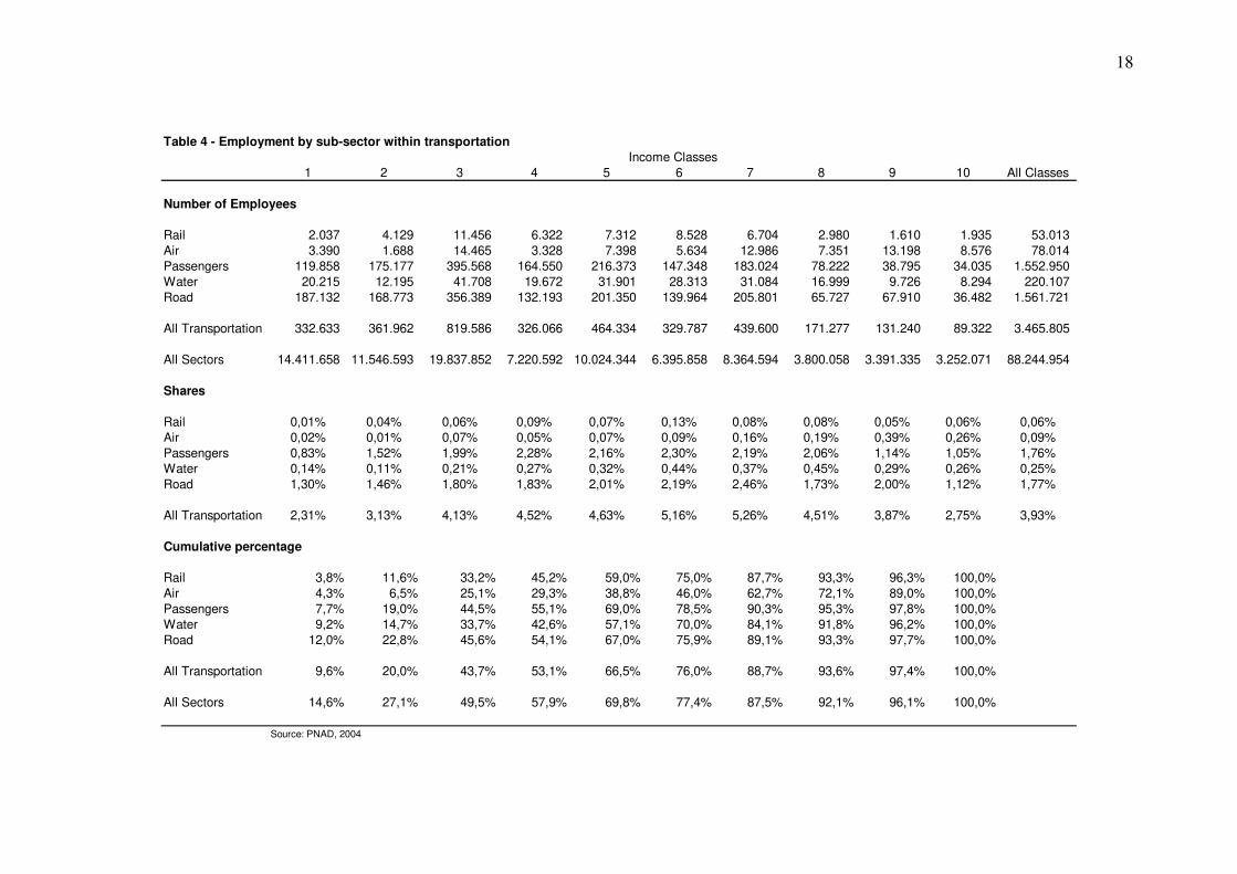
PNAD also provided information on employment by sub-sector within
transportation, which is displayed in Table 4. The total number of jobs in transportation
in general is 3.46 million, the two largest users of labor being road transportation, with
1.561 million employers, and passenger transportation, with 1.553 million. Rail is the
smallest employer, with 53,013 jobs. The aggregate of all sub-sectors is responsible for
3.93% of total employment in Brazil. This share is higher for income classes 3 to 8, and
lower in the two extremes of the distribution, indicating that employment in
transportation is relatively more intense in the middle income classes, especially in
classes 6 and 7.
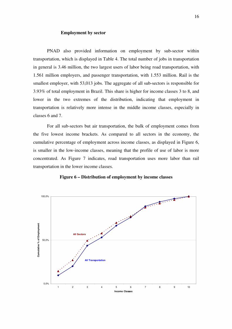
For all sub-sectors but air transportation, the bulk of employment comes from
the five lowest income brackets. As compared to all sectors in the economy, the
cumulative percentage of employment across income classes, as displayed in Figure 6,
is smaller in the low-income classes, meaning that the profile of use of labor is more
concentrated. As Figure 7 indicates, road transportation uses more labor than rail
transportation in the lower income classes.
Figure 6 – Distribution of employment by income classes
Figure 5 - Distribution of employment by income classes
0,0%
50,0%
100,0%
1 2 3 4 5 6 7 8 9 10
Income Classes
Cu
mu
lati
ve %
of
Em
plo
ym
en
t
All Sectors
All Transportation

Source: Table 4
Source: Table 4
17
Figure 7 – Distribution of employment: road x rail
Figure 6 - Distribution of employment: road x rail
0,0%
50,0%
100,0%
1 2 3 4 5 6 7 8 9 10
Income Classes
Cu
mu
lati
ve %
of
Em
plo
ym
en
t
Road
Rail
18
Table 4 - Employment by sub-sector within transportation
1 2 3 4 5 6 7 8 9 10 All Classes
Number of Employees
Rail 2.037 4.129 11.456 6.322 7.312 8.528 6.704 2.980 1.610 1.935 53.013
Air 3.390 1.688 14.465 3.328 7.398 5.634 12.986 7.351 13.198 8.576 78.014Passengers 119.858 175.177 395.568 164.550 216.373 147.348 183.024 78.222 38.795 34.035 1.552.950
Water 20.215 12.195 41.708 19.672 31.901 28.313 31.084 16.999 9.726 8.294 220.107
Road 187.132 168.773 356.389 132.193 201.350 139.964 205.801 65.727 67.910 36.482 1.561.721
All Transportation 332.633 361.962 819.586 326.066 464.334 329.787 439.600 171.277 131.240 89.322 3.465.805
All Sectors 14.411.658 11.546.593 19.837.852 7.220.592 10.024.344 6.395.858 8.364.594 3.800.058 3.391.335 3.252.071 88.244.954
Shares
Rail 0,01% 0,04% 0,06% 0,09% 0,07% 0,13% 0,08% 0,08% 0,05% 0,06% 0,06%
Air 0,02% 0,01% 0,07% 0,05% 0,07% 0,09% 0,16% 0,19% 0,39% 0,26% 0,09%
Passengers 0,83% 1,52% 1,99% 2,28% 2,16% 2,30% 2,19% 2,06% 1,14% 1,05% 1,76%Water 0,14% 0,11% 0,21% 0,27% 0,32% 0,44% 0,37% 0,45% 0,29% 0,26% 0,25%
Road 1,30% 1,46% 1,80% 1,83% 2,01% 2,19% 2,46% 1,73% 2,00% 1,12% 1,77%
All Transportation 2,31% 3,13% 4,13% 4,52% 4,63% 5,16% 5,26% 4,51% 3,87% 2,75% 3,93%
Cumulative percentage
Rail 3,8% 11,6% 33,2% 45,2% 59,0% 75,0% 87,7% 93,3% 96,3% 100,0%
Air 4,3% 6,5% 25,1% 29,3% 38,8% 46,0% 62,7% 72,1% 89,0% 100,0%
Passengers 7,7% 19,0% 44,5% 55,1% 69,0% 78,5% 90,3% 95,3% 97,8% 100,0%Water 9,2% 14,7% 33,7% 42,6% 57,1% 70,0% 84,1% 91,8% 96,2% 100,0%
Road 12,0% 22,8% 45,6% 54,1% 67,0% 75,9% 89,1% 93,3% 97,7% 100,0%
All Transportation 9,6% 20,0% 43,7% 53,1% 66,5% 76,0% 88,7% 93,6% 97,4% 100,0%
All Sectors 14,6% 27,1% 49,5% 57,9% 69,8% 77,4% 87,5% 92,1% 96,1% 100,0%
Source: PNAD, 2004
Income Classes
19
Consumption patterns by sector
The Brazilian household expenditure survey, POF, was implemented in 2002
and 2003. Its information includes monetary and non monetary income, as well as
monetary and non monetary consumption. A total of 48.470 households were
interviewed, and for each one, the sources of income were identified, as well as the
expenditure pattern. Expenditure by households was allocated to 10,429 types of goods
and services in POF 2002/2003. These were aggregated to the 80 types of goods and
services types, presented in the national accounts, and originally used in this study. We
have thus estimated expenditure patterns on 80 different goods and services by each
income class. With this information we were able to identify the consumption patterns
of households in each of the ten income brackets considered in the income distribution
section, for all sectors studied.
Figure 8 presents some information on consumption patterns by income class,
for highly aggregate groups of products. It is clear, as expected, that poorer households
spend a larger percentage of income on Manufactured Food, Manufactured Goods, and
Transportation. These products clearly present decreasing importance on household’s
budget as income increases. On the other hand, Services in General, Services do
Households, Trade, and Communication, present a clear up-ward trend from low to high
income classes.
Transportation refers to household expenditure on this item. It includes
expenditure with urban transportation (bus, taxi, subway, train, boat, and others),
purchase, maintenance and fuel for private vehicles, expenditure on travel (bus, airplane
etc.), parking, toll, parts for vehicles, and insurance. It shows a slight declining trend as
income levels increase, especially after the fourth lowest income class. Considering the
sub-sectors, the share of consumer expenditure on road transportation decreases as
income grows, and increases for air transportation. For rail, the share increases until the
7th income bracket, and then decreases.
This sort of information is available for each sector, allowing for the calculation
of the induced effects of any shock to the system. This provides de direct effects, in the
sense that it portrays the first round of consumer expenditure. The amount spent by poor
households on road transportation, for example, will increase the activity of that sector,

20
which will in turn distribute income to different households. Such income will be spent
in all sectors of the economy, according to the consumption coefficients. The final
effects will include all rounds and dimensions of the production system, and might
differ from the direct ones presented in this section.
Figure 8: Share of different goods services in budget
0,0
0,1
0,2
0,3
0,4
1 2 3 4 5 6 7 8 9 10
Income Classes
Manufactured goods
Manufactured Food
Rent
Transportation
0,0
0,1
0,2
0,3
1 2 3 4 5 6 7 8 9 10
Income Classes
Services to Households
Services
Trade
Communication
Share of Budget
Share of Budget
Source: POF – Pesquisa de Orçamentos Familiares 2002/2003 (IBGE)

21
3.5. Intersectoral relations and income inequality
he information on income distribution by sub-sector within the transportation
sector
ns in Brazil will have
an inco
termine the final impact, which is the profile of
interrel
share o
T
indicates that the rail and road transportation present a similar profile, as can be
seen in Figure 5. In spite of this general observation, the lines indicate that road
transportation distributes income more intensively for the three lowest income classes,
and that rail transportation does so for the 6th, 7th, and 8th classes.
This information indicates that a more intensive use of trai
me concentration impact. However, in order to assess the full impact, other
aspects have to be taken into consideration. Income is distributed to households, which
in turn spend it according to the consumption patterns already shown. The final impact
will depend on which sectors income is spent, regarding their distributive profile.
Income distributed to low-income households might be spent in sectors with a
concentration profile, and vice-versa.
But there is another way to de
ationships between sectors regarding the input-output part of the model. In order
to illustrate that, we present in Table 5 the percentage of purchases made by each sub-
sector within transportation from sectors with lower-than-average inequality. Those
were defined in Moreira et all. (2007), who estimated the final impact in the national
income inequality of identical increases in production in each sector of the economy,
considering the direct, indirect, and induced effects. If the marginal increase in
production produces an inequality index (Gini) lower than the national average, the
sector contributes do diminish inequality, and are labeled pro-poor in this study. Thus,
the table presents the share of purchases from the sub-sectors within transportation
which are made from sectors which promote reduction of inequality.
As can be observed, road cargo transportation is the sub-sector with the lowest
f purchases from pro-poor sectors, 45%. Rail cargo transportation is in the other
extreme, purchasing 68% of its inputs from sectors with interrelationships within the
productive system with sectors that produce lower-than-average income inequality.
Thus, considering this aspect of the problem, it is expected that a change from roads to
rail would promote an improvement in income distribution in the country.
22
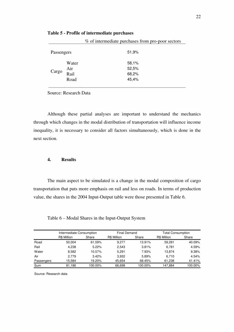
Table 5 - Profile of intermediate purchases
% of intermediate purchases from pro-poor sectors
Passengers 51,9%
Water 58,1%
Air 52,5%
Rail 68,2% Cargo
Road 45,4%
Source: Research Data
Although these partial analyses are important to understand the mechanics
through which changes in the modal distribution of transportation will influence income
inequality, it is necessary to consider all factors simultaneously, which is done in the
next section.
4. Results
The main aspect to be simulated is a change in the modal composition of cargo
transportation that puts more emphasis on rail and less on roads. In terms of production
value, the shares in the 2004 Input-Output table were those presented in Table 6.
Table 6 – Modal Shares in the Input-Output System
R$ Million Share R$ Million Share R$ Million Share
Road 50,004 61.59% 9,277 13.91% 59,281 40.09%
Rail 4,238 5.22% 2,543 3.81% 6,781 4.59%
Water 8,582 10.57% 5,291 7.93% 13,874 9.38%
Air 2,779 3.42% 3,932 5.89% 6,710 4.54%
Passengers 15,584 19.20% 45,654 68.45% 61,238 41.41%
Sum 81,186 100.00% 66,698 100.00% 147,884 100.00%
Source: Research data
Intermediate Consumption Final Demand Total Consumption

23
f 10% of the activity level of road
transport tion to il, and t stressed
that in absolute terms, the simulations transfer a total of R$ 5,928 million, which
represents only 0.17%, of the total production value of the Brazilian economy.
Summary results of the simulations are presented in Tables 7 and 8, while the
detailed results are presented in the appendix.
As Table 7 indicates, the simulated change fr m road to rail will have a small
positiv rsonal income (+0.019%) and on GDP (+0.0026%), and
a negative impact on employment (-0.091%). The positive effect on GDP and personal
income is due to the fact that the intersectoral multiplier for rail is larger than for road
transpo
all aggregate increase in GDP and personal income. An extra R$ million
of road transportation generates a total of 83.4 jobs in the economy (also, direct +
indirect + induced); the same number for rail transportation is 70.0, what explains the
negative impact on employment.
In terms of income distribution, a very small improvement in the Gini index is
istribution. It was also shown, in Section 3.2, that road directly distributes a slightly
ctor contributes to diminish
the positive effect of the intersectoral intermediate purchases. It was also shown that the
income distribution profiles of road and train are quite similar. On balance, the
favorable intermediate consumption effect overcomes the negative effect, producing the
small improvement in the overall income distribution.
Table 8 shows the effects of a change from road to water. The results indicate
that there is practically no change in aggregate personal income (+0.000012%), and a
small improvement in GDP (+0.0043%). Employment decreases by 0.065%. The results
n aggregate GDP are larger than in the simulation of a change from road to rail. For
each R$ of increase in water transportation, there is an increase in aggregate GDP of R$
Two simulations were carried out: a transfer o
a ra he same transfer to water transportation. It should be
o
e impact on aggregate pe
rtation. For each R$ of increase in road transportation, there is an increase in
aggregate GDP of R$ 1.895, considering direct, indirect and induced effects. The same
number for rail transportation is slightly larger, R$ 1.903. These small differences
explain the sm
observed (in the tenth digit after the decimal point). Rail transportation is the sector with
the largest share of intermediate purchases from pro-poor sectors, as shown in Section
3.5, meaning that the indirect effects contribute to an improvement in income
d
higher percentage of income to the lower classes, and this fa
o

24
1.909, considering direct, indirect and induced effects, slightly larger than the number
for road and also rail transportation. An extra R$ million of water transportation
generates a total of 73.9 jobs in the economy (direct + indirect + induced), smaller than
the number of jobs created by road transportation (83.4), explaining the aggregate
e previous case, there is also a very small
prov al
e
the
Person
decrease in employment.
In terms of income distribution, as in th
im ement, as measured by the Gini index (also in the tenth digit after the decim
point). The case is similar to the change from road to rail: water transportation buys a
larger share of intermediate inputs than road from pro-poor sectors (58.1% versus
45.4%), and distributes slightly less direct income to the lower classes. Again, th
positive effect on income inequality of pro-poor intermediate purchases overcomes
negative impact of direct income distribution.
Table 7 - Impacts Overall the Economy of a Transfer of 10% of the Activity Level
in the Road System to the Rail System
Before After Change Change
Values %
al Income a
1,255,042 1,255,284 242 0.019%
GDP a
1,941,498 1,941,548 50 0.0026%
Employment b
88,244,954 88,164,235 -80,719 -0.091%
GINI Index c
0.4860704672 0.4860704671 -0.0000000001 -0.000000014%
Notes: a. R$ Million; b. number of persons; c. the value of the Gini index differs from the
official figures, because it was estimated taking into consideration the
input-output system.
Source: Research data

25
Table 8 - Impacts Overall the Economy of a Transfer of 10% of the Activity Leve
in the Road System to the Waterways System
Before After Change Change
Values %
Personal Income a
1,255,042
l
1,255,042 0.16 0.000012%
GDP a
1,941,498 1,941,582 84 0.0043%
Employment b
88,244,954 88,187,862 -57,092 -0.065%
GINI Index c
0.486070467196 0.486070467203 0.00000000001 0.0000000015%
Notes: a. R$ Million; b. number of persons; c. the value of the Gini index differs from the
official figures, because it was estimated taking into consideration the
input-output system.
Source: Research data
Conclusions
The goal of this work is to measure the income distribution effects of changes in
of cargo transportation in Brazil. A Lethe modal composition ontief-Miyazawa type
model with a base year 2004 was constructed, disaggregated into 31 sectors (4 of which
related to cargo transportation: road, rail, water, and air), and 10 income brackets.
Transfers of 10% of the activity level of road transportation either to rail or to
water transportation were simulated, and the results presented impacts on GDP,
aggregate income, employment and Gini index changes. Since the system is linear, the
direction of the changes will not change with the size of the percentage of activity
changed from road to other transportation modes, although the sizes of the impacts will
vary.
The results show that the relative impacts are small, considering the relative size
of the change simulated in relation to the Brazilian economy. Increases in the share of
rail or water transportation will be better for GDP, personal income and income
distribution, but it will decrease employment. Increases in the share of rail
transportation will have more positive effects on personal income and income
distribution than increases in the share of water transportation. A change to water will
result in a larger GDP change and a smaller number of jobs lost in comparison to a
change to rail. These results are explained by the lower direct employment coefficients

26
of rail and water (26.3 for road, 7.8 for rail, and 15.9 for water) and by their lower
ent generators (83.4 for road, 70.0 for rail, and 73aggregate employm .9 for water).
This study focused only on the distributional aspects of possible changes in the
modal composition of cargo transportation in Brazil, without consideration of aggregate
efficiency and price changes, aspects that are beyond the scope of this work. Possible
efficiency improvements due to changes in the modal composition can lead to increased
aggregate production and changes in the sectoral structure of the economy, since
different sectors rely differently on distinct modes of transportation and, therefore, will
not be affected equally. Given the present sectoral structure, the direction of the effects
are the ones presented above. In general, a reduction in the share of road transportation
ill produce positive impacts in GDP, personal income, and income distribution, but
impacts on employment.
References
Gol
Gui de v. 9,
n. 2
Kale
Kale
Key
Leontief, W. W. (1951). The Structure of the American Economy. Second Enlarged Edition. New York: Oxford University Press.
Miy awa,
Miy
Miyazawa, K. (1960). "Foreign Trade Mult
Mor
w
will produce negative
dberg, S. (1958). Introduction to Difference Equations. New York: Wiley.
lhoto, J. and Sesso-Filho, U. (2005). “Estimação da Matriz Insumo-Produto a partirDados Preliminares das Contas Nacionais”. Economia Aplicada, São Paulo, SP,
.
cki, M. (1968). Theory of Economic Dynamics. New York: Monthly Review Press.
cki, M. (1971). Selected Essays on the Dynamics of the Capitalist Economy. Cambridge: Cambridge University Press.
nes, J. M. (1936). The General Theory of Employment, Interest, and Money. New York: Harcourt. 1964.
az K. (1963). "Interindustry Analysis and the Structure of Income Distribution." Metroeconomica, Aug.-Dec., vol. 15, nos. 2-3.
azawa, K. (1976). Input-Output Analysis and the Structure of Income Distribution. Berlin: Springer-Verlag.
iplier, Input-Output Analysis and the Consumption Function." Quaterly Journal of Economics, Feb., vol. 74, no. 1.
eira, G., Almeida, L., Guilhoto, J. and Azzoni, C. (2007) Productive Structure and Income Distribution: The Brazilian Case, Quarterly Review of Economics and
Finance (http://dx.doi.org/10.1016/j.qref.2006.12.010)
ng, G. (1980). Linear Algebra and Its Applications. 2nd. ed.. New York: Academic StraPress.
Recommended


![[Harmonia] Ron Miller - Modal Jazz Composition & Harmony - Vol 2](https://img.pdfslide.us/doc/110x75/56d6bfa81a28ab3016971edf/harmonia-ron-miller-modal-jazz-composition-harmony-vol-2.jpg)