Mixed integer rounding cuts and master group polyhedra
Sanjeeb Dash∗
June 23, 2011
Abstract
We survey recent research on mixed-integer rounding (MIR) inequalities and a generalization,
namely the two-step MIR inequalities defined by Dash and Gunluk (2006). We discuss the
master cyclic group polyhedron of Gomory (1969) and discuss how other subadditive inequalities,
similar to MIR inequalities, can be derived from this polyhedron. Recent numerical experiments
have shed much light on the strength of MIR inequalities and the closely related Gomory mixed-
integer cuts, especially for the MIP instances in the MIPLIB 3.0 library, and we discuss these
experiments and their outcomes. Balas and Saxena (2007), and independently, Dash, Gunluk
and Lodi (2007), study the strength of the MIR closure of MIPLIB instances, and we explain
their approach and results here. We also give a short proof of the well-known fact that the MIR
closure of a polyhedral set is a polyhedron. Finally, we conclude with a survey of the complexity
of cutting-plane proofs which use MIR inequalities.
This survey is based on a series of 5 lectures presented at the Seminaire de mathematiques
superieures, of the NATO Advanced Studies Institute, held in the University of Montreal, from
June 19-30, 2006.
1 Introduction
Over the last 10-15 years, cutting planes have emerged as a vital tool in mixed-integer programming.
We call a linear inequality satisfied by all integer points in a polyhedron P a cutting plane (or cut)
for P . Most commercial software which solve mixed-integer programs, such as ILOG-CPLEX [63]
or XPRESS-MP [89], use sophisticated algorithms to find cutting planes and combine them with
linear programming based branch-and-bound in a branch-and-cut system. There is a lot of literature
on problem-specific cutting planes; in the context of the traveling salesman problem (TSP) for
example, comb inequalities are very useful in solving TSP instances to optimality. In this survey,
we will mainly discuss cutting planes for general (mixed) integer programs. That is, we will not
assume any underlying combinatorial structure. In such cases, the mixed-integer rounding (MIR)
inequalities (or MIR cut) and the closely related Gomory mixed-integer (GMI) cuts form the most
important class of cutting planes.
The GMI cut was derived by Gomory in 1960 [54]. After some initial limited experimentation,
these cuts were hardly used to solve mixed-integer programs for a long time. One exception is
the paper of Geoffrion and Graves [51] in 1974 who described a successful combination of GMI
∗IBM T.J. Watson Research Center, P.O. Box 218, Yorktown Heights, NY 10598, [email protected]
1

cuts with LP based branch-and-bound to solve MIPs. In particular, they used a “hybrid branch-
and-bound/cutting-plane approach” where “the cuts employed are the original mixed integer cuts
proposed by Gomory in 1960, and are applied to each node problem in order to strengthen the
LP bounds”. They used the above ideas to solve a pure 0-1 integer program with several hundred
binary variables. Some of the implementation ideas in this paper anticipate the (independent) work
of Balas, Ceria, Cornuejols and Natraj [14], who performed a systematic study of GMI cuts and
popularized them as a tool for general mixed-integer programs in the 1990s. See [29] for additional
historical information. Subsequent computational studies [18] confirmed the usefulness of the GMI
cut for practical mixed-integer programs.
Nemhauser and Wolsey [76, p.244] introduced mixed-integer rounding inequalities, or cutting
planes that can be produced by what they call the MIR procedure. These authors later [77] strength-
ened and redefined the MIR procedure and the resulting inequality; see [39] for a discussion on the
development of MIR inequalities. They also showed that the MIR inequality, the GMI cut, and
the split cut were equivalent. Split cuts were defined by Cook, Kannan and Schrijver [28], and are
a special case of the disjunctive cuts introduced by Balas [12]. Marchand and Wolsey [72] later
showed that many cuts in the literature are special cases of the MIR cut. They also computationally
established the usefulness of the MIR cut; the MIR cuts in their experiments are different from the
GMI cuts used in [14, 18]. The definition of the MIR cut we use in this paper is equivalent to the
one in [77], though our presentation is based on [88]. By the late 1990s, the importance of the GMI
cut and the MIR cut in solving mixed-integer programs was clear, and these cuts have become a
standard feature of major commercial MIP solvers.
Gomory [55] introduced group relaxations of integer programs. Some computational studies of
group relaxations can be found in White [87], Shapiro [84], and Gorry, Northup and Shapiro [60]. The
latter paper contains a study of a group relaxation based branch-and-bound algorithm. After some
initial work on this topic, by the mid-1970s, group relaxations were not viewed as a central technique
to solve integer programs (see [52]). In his important work on polyhedral properties of group
relaxations, Gomory [56] studied corner polyhedra (the convex hull of solutions of group relaxations)
and the related cyclic group polyhedra. He highlighted the role of subadditive functions in obtaining
cutting planes for corner polyhedra and for MIPs, and derived the GMI cut for pure integer programs
from a facet of the master cyclic group polyhedron (MCGP). GMI cuts for mixed-integer programs
can similarly be derived from the mixed-integer extension of the MCGP; see Gomory and Johnson
[57]. The MCGP has a rich polyhedral structure and it is natural to ask if it has other facets
that would lead to useful cutting planes for mixed-integer programs. We call such cuts group cuts.
Following recent work on this topic by Gomory, Johnson and co-authors in [8] and [59], cyclic group
polyhedra and group cuts are an active area of study; see [35]–[41].
An active research topic is the computational study of the strength of closures (or elementary
closures) of different families of cutting planes. For a family of cutting planes F , and a polyhedron P ,
the closure is the set of all points in P satisfying the cutting planes in F . Chvatal [24] rediscovered
Gomory cuts (we call them Gomory-Chvatal cuts (GC) in this paper) and initiated the study of the
Chvatal closure, i.e., the closure with respect to Gomory-Chvatal cuts. A computational study of the
Chvatal closure can be found in a recent paper by Fischetti and Lodi [47]. They framed the problem
of separating a point from the Chvatal closure, or equivalently, of finding a violated GC cut, as an
MIP (such an MIP can also be found in Bockmayr and Eisenbrand [19]). See [62] for related work on
verifying that an inequality has Chvatal rank 1 or 2. Fischetti and Lodi used a standard MIP solver
2
to find violated GC cuts and approximately optimized over the Chvatal closure of MIP instances in
the MIPLIB 3.0 problem set. This procedure is computationally intensive, but yields strong bounds
for many of the pure integer instances in MIPLIB, in contrast to using Gomory cuts derived from
optimal simplex tableau rows, as attempted in earlier papers on this topic. Independently, Bonami
and Minoux [21] approximately optimized over the closure with respect to lift-and-project cuts for
0-1 MIP instances from MIPLIB 3.0. Recently Bonami et. al. [20] optimized over the closure of
projected GC cuts for the mixed-integer instances from MIPLIB using an MIP solver to find violated
cuts. GC cuts and lift-and-project cuts are both special cases of split/MIR cuts. Motivated by the
above work, Dash, Gunluk and Lodi [39] and independently, Balas and Saxena [16] approximately
optimize over the MIR closure of MIP instances, and show that a large fraction of the integrality
gap can be closed in this way for MIPLIB 3.0 instances. However, it takes (in these papers) much
more time to optimize over the closures above than to solve the original MIP (with few exceptions,
as noted in [47], [16]). This is not surprising as it is NP-hard to separate an arbitrary point from
the Chvatal closure [42], or from the split closure [23] (though one can solve an LP to find a violated
lift-and-project cut).
Besides their usefulness in practice, cutting planes have some very interesting theoretical prop-
erties. Many statements with a combinatorial flavor, such as “the maximum size clique in a specific
graph G has fewer than 10 nodes”, can be proved by a Gomory-Chvatal cutting-plane proof, or a
sequence of GC cuts, where each one is obtained from some original constraints modeling the com-
binatorial problem and the previous GC cuts. This is a consequence of Gomory’s result [53] on the
finite termination of his cutting plane algorithm for solving integer programs. Pudlak [78] showed
that for 0-1 integer programs without integer solutions, GC cutting-plane proofs certifying their
infeasibility have exponentially many cuts in the worst case. A similar result for MIR cutting plane
proofs was recently proved in [33].
In this paper, we survey recent work on MIR cuts and cyclic group polyhedra. We start off with
a simple extension of MIR cuts, namely the two-step MIR cuts in Dash and Gunluk [36], a parametric
family of group cuts. We then discuss fundamental properties of Gomory’s cyclic group polyhedra,
including Gomory’s characterization of the convex hull of non-trivial facets of these polyhedra in
Section 3. We further discuss some important facets of these polyhedra, and their relationship
to subadditive functions, and to valid inequalities for mixed-integer programs. We move on (in
Section 4) to a discussion of the MIR closure of a polyhedral set, and present a short proof that the
MIR closure is a polyhedron, based on (but different from) a recent proof in Dash, Gunluk, and Lodi
[39]. This result follows from the result of Cook, Kannan and Schrijver [28] that the split closure
of a polyhedral set is a polyhedron. We also present the MIP model from [39] to find violated MIR
cuts. In Section 5, we discuss computational work on using cyclic group polyhedra to solve integer
programs. We discuss recent studies on the computational effectiveness of two-step MIR cuts in
Dash, Gunluk and Goycoolea [35], and interpolated group cuts in Fischetti and Saturni [49]. We also
discuss computational studies of the strength of the MIR closure. Finally, in Section 6, we discuss
a recent result from [33] that shows that an MIR cutting plane proof certifying that an infeasible
integer program has no integral solutions can have exponentially many cuts in the worst case.
3

2 The MIR inequality and extensions
Consider the set
P = v ∈ Rl, x ∈ Z
n : Cv + Ax = d, v, x ≥ 0, x integer.
By a mixed-integer program, we mean the problem of minimizing a linear function gv+hx subject to
(v, x) ∈ P , where g ∈ Rl, h ∈ R
n, and gv and hx stand for the inner products between the respective
vectors. We denote the continuous relaxation of P by PLP , and the convex hull of P by conv(P ).
We will study valid inequalities for P , or (equivalently) cutting planes for PLP . We assume that all
numerical data is rational. Let
Q =v ∈ R
|J|, x ∈ Z|I| :
∑
j∈J
cjvj +∑
i∈I
aixi = b, v, x ≥ 0,
where the equation defining Q is obtained as a linear combination of the equations defining P ,
and I and J are index sets of the integer/non-integer variables. In other words, a = λT A, c =
λT C and b = λT d for some real vector λ of appropriate dimension. As P ⊆ Q, valid inequalities
for Q yield valid inequalities for P . For a valid inequality derived in this way, we will refer to∑j∈J cjvj +
∑i∈I aixi = b as its base equation. Finally, for a number v, let v stand for v − ⌊v⌋, the
fractional part of v.
2.1 The MIR inequality
There are many equivalent ways of defining the MIR inequality; see [39]. The presentation here is
based on the presentation in the book [88] by Wolsey. Define
Q1 =v ∈ R, z ∈ Z : v + z ≥ b, v ≥ 0
.
The basic mixed-integer inequality, defined in [88] as
v + bz ≥ b⌈b⌉, (1)
is valid and facet-defining for Q1.
Lemma 1 conv(Q1) =v, z ∈ R : v + z ≥ b, v + bz ≥ b⌈b⌉, v ≥ 0
.
Proof The result is trivial if b = 0; so assume b 6= 0. Let Q′ be the set on the right-hand side of the
equation in Lemma 1. Let (v, z) ∈ Q1. If z ≥ ⌈b⌉, then v ≥ 0 implies that v + bz ≥ b⌈b⌉. If z ≤ ⌊b⌋,
then v + z ≥ b implies that
v ≥ b + ⌊b⌋ − z ≥ b + b(⌊b⌋ − z) = b(⌈b⌉ − z).
Therefore, (1) is a valid inequality for Q1 and conv(Q1) ⊆ Q′. On the other hand, the extreme
points of Q′ are (0, ⌈b⌉) and (b, ⌊b⌋), given by the intersections of the first and third inequalities with
the second inequality. Both these points lie in Q1, and thus Q′ ⊆ conv(Q1).
In Figure 1(a), we depict the points in Q1 by horizontal lines. In Figure 1(b), the half-plane
above the dashed line represents (1), and contains the shaded regions which are Q1 ∩ z ≤ ⌊b⌋ and
4

z
v
z
b
v
Figure 1: The basic mixed-integer inequality
Q1 ∩ z ≥ ⌈b⌉. If b is not integral (i.e., b 6= 0), then the point (v, z) = (0, b) violates the basic
mixed-integer inequality.
An approach to deriving valid inequalities for more general sets defined by a single inequality
is to combine variables to get a structure resembling Q0. For example, consider Q, and a set S ⊆ I.
We can relax the equation defining Q by rounding up the coefficients of xi for i ∈ I \S, and dropping
continuous variables with negative coefficients to obtain
∑
cj>0
cjvj +∑
i∈S
ai xi +∑
i∈I\S
⌈ai⌉ xi ≥ b, (2)
as a valid inequality for Q. Writing ai = ⌊ai⌋ + ai for i ∈ S, and re-arranging terms, we get
( ∑
cj>0
cjvj +∑
i∈S
ai xi
)+
(∑
i∈S
⌊ai⌋ xi +∑
i∈I\S
⌈ai⌉ xi
)≥ b. (3)
The first part of this inequality is non-negative, and the second part is integral for all (v, x) ∈ Q.
Therefore, the basic mixed-integer inequality implies that
( ∑
cj>0
cjvj +∑
i∈S
ai xi
)+ b
( ∑
i∈S
⌊ai⌋ xi +∑
i∈I\S
⌈ai⌉ xi
)≥ b⌈b⌉. (4)
is valid for Q. The coefficients of xi in this inequality are b⌊ai⌋ + a if i ∈ S, and b⌈ai⌉ if i ∈ I \ S.
Therefore, S = i ∈ I : ai ≤ b gives the strongest inequality of this form, which is
∑
cj>0
cjvj +∑
i∈I:ai≤b
(b⌊ai⌋ + ai)xi +∑
i∈I:ai>b
b⌈ai⌉xi ≥ b⌈b⌉. (5)
We call (5) the mixed-integer rounding inequality for Q. Note that the coefficients of xi can be written
as b⌊ai⌋ + minai, b. Finally, as observed by Cornuejols, Li, and Vandenbussche [30], scaling the
the equation defining Q by a rational number t before writing the MIR inequality, can be useful in
some circumstances. We call such an inequality a t-scaled MIR inequality.
Assume b 6= 0. Subtracting b times∑
j∈J cjvj +∑
i∈I ai xi = b from the MIR inequality, and
dividing by (1 − b), we get the equivalent inequality:
∑
j∈J:cj>0
cjvj −∑
j∈J:cj<0
b cj
1 − bvj +
∑
i∈I:ai≤b
aixi +∑
i∈I:ai>b
b(1 − ai)
1 − bxi ≥ b, (6)
This is the Gomory mixed-integer cut, as originally defined in [54].
5

To define the MIR inequality for P , we start off with some multiplier vector λ and define
c = λT C, a = λT A, and b = λT d. Then cv + ax = b is a valid inequality for P , and we call (5) an
MIR inequality for P . Define the MIR rank of an inequality valid for PLP to be 0. For an inequality
valid for P , define the MIR rank to be a positive number t if it does not have MIR rank t−1 or less,
but is a non-negative linear combination of MIR inequalities derived from inequalities with MIR
rank t − 1. All cutting planes for a pure integer program have finite MIR rank, but this is not true
in the case of mixed-integer programs [28].
A linear inequality gv + hx ≥ q is called a split cut for P if it is valid for both PLP ∩ αx ≤ β
and PLP ∩ αx ≥ β + 1, where α and β are integral. The inequality gv + hx ≥ q is said to be
derived from the disjunction αx ≤ β ∨ αx ≥ β + 1. All points in P satisfy any split cut for P . The
basic mixed-integer inequality is a split cut for Q1 derived from the disjunction z ≤ ⌊b⌋ and z ≥ ⌈b⌉,
when b 6= 0. Therefore, the MIR inequality (5) is a split cut for P . Nemhauser and Wolsey [77]
showed that every split cut for P is also an MIR inequality; more precisely, given a split cut, there is
an MIR cut which is equivalent to it in the sense that it differs from the split cut by some multiple
of the equations Cv + Ax = d.
The derivation of the MIR inequality can be viewed as a special case of the following approach.
Consider a linear transformation
T : Q → Q′ = v, z ∈ R :
(v′
z′
)= U
(v
x
)+ l ⊆ Q1,
where U is a matrix, l is a vector. If αT(v′
z′
)≥ β is valid for Q′, then αT U
(vx
)+ αT l ≥ β is valid
for Q. In the case of the MIR inequality, l = 0, and the coefficients in the first and second rows
of U are defined, respectively, by the coefficients in the first and second bracketed expressions in
(3). This approach is used in local cuts for the TSP by Applegate et. al. [7] with varying linear
transformations into varying sets, and not a fixed set such as Q1. The transformations in [7] are
defined by the operation of shrinking sets of nodes to single nodes, and thus have a combinatorial
nature, unlike the somewhat abstract transformations in the case of the MIR inequality.
Subsequent to the work of Wolsey [88], and Marchand and Wolsey [72], deriving (or explaining)
valid inequalities for mixed-integer programs in the above manner, starting from valid inequalities
for very simple polyhedral sets became an active research topic. For example, let∑
i∈I αixi ≥ β
be a valid inequality for P . Then∑
i∈I⌈αi⌉xi ≥ ⌈β⌉ is valid for P , and is called a Gomory-Chvatal
cut if P has no continuous variables, and a projected Chvatal-Gomory cut [20] otherwise. The above
inequality can be derived by mapping P into the set Q0 = z ∈ Z : z ≥ β via the mapping
z =∑
i∈I⌈αi⌉xi, and then using the only facet-defining inequality of Q0, namely z ≥ ⌈β⌉. Gunluk
and Pochet [61] define the mixing-mir inequalities from facets of the set (x, z) ∈ R × Zn : x + zi ≥
bi, for i = 1, . . . , n, x ≥ 0. The underlying motivation behind such research in the context of
mixed-integer programming and in local cuts for the TSP is that strong (facet-defining) inequalities
for simple sets defined on few variables yield useful inequalities for problems with many variables.
The hard part is to find the appropriate small sets and linear transformations. In recent work,
Espinoza [44] generated linear transformations dynamically, in a manner similar to the work in [7],
to find useful cutting planes for Q, though with moderate success.
6

2.2 Two-step MIR inequalities
In the relaxation of Q in (2), the coefficient ai of an integer variable xi is either unchanged or
rounded up to ⌈ai⌉. One can get different cuts for Q by increasing ai to a number less than ⌈ai⌉,
say ⌊ai⌋ + α where 0 < α < 1, thereby obtaining a stronger relaxation than (2).
Dash and Gunluk [36] obtained such cuts from a simple mixed-integer set with three variables:
Q2 =v ∈ R, y, z ∈ Z : v + αy + z ≥ β, v, y ≥ 0
,
where α, β ∈ R are parameters that satisfy 1 > β > α > 0, and ⌈β/α⌉ > β/α. Though β is required
to be less than 1 in Q2, the fact that z can take on negative values makes the set fairly general. We
do not know of an explicit description of the convex hull of points in Q2; however one can obtain
the inequalities describing the convex hull in polynomial time using results in [11] and [3]. Dash
and Gunluk showed that the following inequalities are valid for Q2, and facet defining under some
conditions:
v + αy + βz ≥ β, (7)(1/(β − α ⌊β/α⌋)
)v + y + ⌈β/α⌉ z ≥ ⌈β/α⌉ . (8)
Lemma 2 [36] The inequality (7) is valid and facet-defining for Q2. If 1/α ≥ ⌈β/α⌉, then the
inequality (8) is valid and facet-defining for Q2.
Proof The inequality (7) can be obtained by treating v + αy as a continuous variable and applying
the basic mixed-integer inequality (1) to (v + αy) + z ≥ β. To see that inequality (8) is valid,
notice that the inequalities
(1/α)v + y + (β/α)z ≥ β/α,
(1/α)v + y + (1/α)z ≥ β/α,
are valid for Q2. Therefore, for any γ ∈ R satisfying 1/α ≥ γ ≥ β/α, the inequality
(1/α)v + y + γz ≥ β/α
is also valid as it can be obtained as a convex combination of valid inequalities. If 1/α ≥ ⌈β/α⌉,
then
v/α + y + ⌈β/α⌉ z ≥ β/α (9)
is valid for Q2. Applying (1) to the previous inequality with v/α treated as a continuous variable
and y + ⌈β/α⌉ z treated as an integer variable gives inequality (8). Consider the following points in
Q2:
p1 = (0, 0, 1), p2 = (0, ⌈β/α⌉ , 0), p3 = (β − α ⌊β/α⌋ , ⌊β/α⌋ , 0), p4 = (β, 0, 0).
As depicted in Figure 2, the points p1, p3 and p4 are affinely independent and tight for (7). Also,
the affinely independent points p1, p2 and p3 are tight for (8), and thus these two inequalities are
facet-defining for Q2.
We call (8) the two-step MIR inequality for Q2; it is obtained by applying (1) twice, and has MIR
rank at most two. The inequalities (7) and (8) are not necessarily sufficient to describe the convex
7

1
x
z
y
base inequality
p
2
x
z
y
two−step MIR
MIR
p
p
3
p
4
Figure 2: Some facets of Q2
hull of Q2. However, let Q2+ = Q2 ∩ z ≥ 0; (7) and (8), along with the inequalities v, x, z ≥ 0,
define the convex hull of integer solutions of Q2+ [36]. The additional restriction 1/α ≥ ⌈β/α⌉ is not
required. Conforti and Wolsey [25] characterized the convex hull of a generalization of Q2+ (and of
Q2+) which they call X2DIV . They assume all variables are non-negative and thus their results do
not imply Lemma 2. We note that if 1/α ≤ ⌈β/α⌉ (1/α = ⌈β/α⌉), inequality (8) is an (1/α)-scaled
MIR inequality for Q2+ (Q2). Thus, it is only when 1/α > ⌈β/α⌉ that the two-step MIR inequality
can have MIR rank 2.
We illustrate the use of inequality (8) in an example. Consider the equation 3.35x1 + 2.5x2 −
1.2x3 = 4.7 with all variables non-negative and integral. This equals .35x1 + .5x2 + .8x3 + w = .7,
where w = 3x1 + 2x2 − 2x3 − 4. Here β = 0.7; let α = 0.4. Then 1/α = 2.5 > ⌈β/α⌉ = 2. As
x1, x3 ≥ 0, the inequality (.1x2)+ .4(x1 +x2)+(x3 +w) ≥ .7 is a relaxation of the previous equation.
Of the three terms in brackets, the first two are non-negative, and the last two are integral; we can
thus apply inequality (8) to obtain the valid inequality: (1/2)x1 + (2/3)x2 + x3 + w ≥ 1.
We now formalize this procedure to obtain valid inequalities for Q. Let β = b, and choose
α ∈ (0, b) such that 1/α ≥ ⌈b/α⌉. Define τ = ⌈b/α⌉ ≥ 2, and define ρ = b − α⌊b/α⌋. Let ki, li be
integers such that ki ≤ ⌊ai/α⌋, and li ≥ ⌈ai/α⌉, for i ∈ I. Let I0, I1 and I2 be sets which form a
partition of I, and let w =∑
i∈I⌊ai⌋xi − ⌊b⌋. We can relax the equation in Q to obtain∑
cj>0
cjvj +∑
i∈I1
(kiα + (ai − kiα))xi +∑
i∈I2
liα xi +∑
i∈I0
xi + w ≥ b,
which can be rewritten as
∑
cj>0
cjvj +∑
i∈I1
(ai − kiα)xi + α( ∑
i∈I1
ki xi +∑
i∈I2
li xi
)+
( ∑
i∈I0
xi + w)
≥ b,
We can map points in Q to points in Q2 by equating the first variable in Q2 with the sum of the
first two terms in the equation above, and equating the second and third variables with the first and
second bracketed expressions, respectively. Applying inequality (8) and substituting for w leads to
inequality ∑
cj>0
cjvj +∑
i∈I
γixi + ρ τ z ≥ ρ τ ⌈b⌉, (10)
where γi = ρ τ ⌊ai⌋ +
ρ τ if i ∈ I0,
kiρ + ai − kiα if i ∈ I1,
liρ if i ∈ I2.
8

By inspection, the strongest inequality of this form is obtained by setting ki = k∗i = ⌊ai/α⌋ and
li = l∗i = ⌈ai/α⌉ for i ∈ I, and letting
I0 = i ∈ I : ai ≥ b,
I1 = i ∈ I \ I0 : ai − k∗i α < ρ, I2 = i ∈ I \ I0 : ai − k∗
i α ≥ ρ.
In other words,
γi = ρ τ ⌊ai⌋ + minρ τ , k∗i ρ + ai − k∗
i α , l∗i ρ .
As shown in [36], these inequalities imply the strong fractional cuts of Letchford and Lodi [70]. They
can be separated in polynomial time, under some restrictions.
Theorem 3 (Dash, Goycoolea, Gunluk [35]) Given a point (v∗, x∗) ∈ QLP , the most violated two-
step MIR inequality can be found in polynomial time, assuming τ ≤ k for some fixed k.
Here, the violation of (10) with respect to (v∗, x∗) is given by its right-hand side minus the left-hand
side evaluated at (v∗, x∗). The algorithm given in [35] is very simple; just write down the inequality
(10) for all feasible choices of α from the set ai/t : i ∈ I, t ∈ N, ai/t ≥ b/k ∪ 1/t : t ∈ N, tb ≤ k,
and compute the violation.
Kianfar and Fathi [64] generalize the two-step MIR inequalities and generate n-step MIR in-
equalities for Q. These inequalities have MIR rank at most n.
3 Master polyhedra
Gomory [56] developed the concepts of corner polyhedra and master polyhedra as tools to generate
cutting planes for general integer programs, and to solve asymptotic integer programs. We do not
discuss the latter aspect here. The corner polyhedron (strengthened corner polyhedron) for a vertex
of PLP is the convex hull of integer points satisfying only the n linearly independent constraints
which define the vertex (all constraints tight at the vertex). Clearly, valid inequalities for a corner
polyhedron of P yield valid inequalities for P . The central element of Gomory’s approach is the fact
that many different corner polyhedra can be viewed as faces of a much smaller number of master
polyhedra, which are much more ‘regular’ and amenable to analysis. Gomory, and later Gomory
and Johnson [57] showed how to obtain facets of master polyhedra, which yield valid inequalities
for corner polyhedra and thereby for P . In this section, we describe in detail master cyclic group
polyhedra, or master polyhedra associated with corner polyhedra for single constraint (plus non-
negativity of variables) systems, such as the one defining Q. Many results are available for such
polyhedra, but master polyhedra for multiple constraint systems are less well-understood, beyond
the initial results of Gomory. We briefly discuss some recent research on this topic later.
For the set Q, assume that ai (i ∈ I) and b are rational numbers with a common denominator
n, and let b = r/n, where 0 < r < n. Rewrite Q as
Q =
v ∈ R|J|, x ∈ Z
|I| : (∑
i∈I
⌊ai⌋xi − ⌊b⌋) +∑
j∈J
cjvj +∑
i∈I
ai xi = b, v, x ≥ 0
9

Let Ik = i ∈ I : ai = k/n and define the mapping
wk =∑
i∈Ikxi, z = −(
∑
i∈I
⌊ai⌋xi − ⌊b⌋)
v+ =∑
cj>0 cjvj , v− = −∑
cj<0
cjvj , (11)
that maps each point (v, x) in Q to a point (v+, v−, w) in the polyhedron
P ′(n, r) = convv+, v− ∈ R, w ∈ Zn−1 : v+ − v− +
n−1∑
i=1
i
nwi − z =
r
n, v+, v−, w ≥ 0, z ∈ Z.
(If Ik is empty for some k, set wk to zero.) If Q has no continuous variables, then (11) maps points
in Q to points in the master cyclic group polyhedron of Gomory:
P (n, r) = conv w ∈ Zn−1 :
n−1∑
i=1
i
nwi − z =
r
n, w ≥ 0, z ∈ Z. (12)
We view P ′(n, r) as the mixed-integer extension of P (n, r). For P (n, r), z can be assumed to be
non-negative, but not for P ′(n, r). Note that the constraint defining P (n, r) can be written as∑n−1i=1 iwi ≡ r (mod n). In [54], Gomory first derived the GMI cut as a valid inequality for points
satisfying a similar equation.
Recently, Dash, Fukasawa and Gunluk [34] studied the polyhedron
K(n, r) = conv (x, y) ∈ Zn × Z
n :
n∑
i=1
ixi −
n∑
i=1
iyi = r, x, y ≥ 0 (13)
where n, r ∈ Z and 0 < r ≤ n, and characterized the convex hull of its non-trivial facets. K(n, r) was
first defined by Uchoa [85] in a slightly different form. Replacing z in (12) by yn, and multiplying
the defining constraint by n, we see that P (n, r) defines a face of K(n, r). Facets of P (n, r) can be
lifted to obtain facets of K(n, r), but not all facets can be obtained this way [34].
3.1 Basic properties
Both P (n, r) and P ′(n, r) are full-dimensional, unbounded polyhedra, and their characteristic (re-
cession) cones are Rn−1+ and R
n+1+ respectively. Also, the inequalities xi ≥ 0 for i = 1, . . . , n − 1
define facets for both P (n, r) and P ′(n, r), and the inequalities v− ≥ 0 and v+ ≥ 0 are facet-defining
for P ′(n, r). Therefore, if ηT w ≥ ηo is a facet defining inequality of P (n, r), then η, ηo ≥ 0. Further,
for any nontrivial facet (i.e., not defined by the non-negativity inequalities), ηo > 0. We will assume
in what follows that ηo is scaled to be 1. Finally, any nontrivial facet of P (n, r) has the following
property: there is a set of n − 1 linearly independent integer points χi in P (n, r) satisfying χii ≥ 1,
for i = 1, . . . , n − 1. Gomory characterized the convex hull of nontrivial facets of P (n, r).
Theorem 4 [56] If r 6= 0, then∑n−1
i=1 ηiwi ≥ 1 is a non-trivial facet of P (n, r) if and only if η = (ηi)
is an extreme point of the inequalities
ηi + ηj ≥ η(i + j)mod n ∀i, j ∈ 1, . . . , n − 1, (14)
ηi + ηj = ηr ∀i, j such that r = (i + j)mod n, (15)
ηj ≥ 0 ∀j ∈ 1, . . . , n − 1, (16)
ηr = 1. (17)
10

The property (14) is called subadditivity.
Gomory actually proved a more general result. Consider an integer k > 0, and let r, n ∈ Zk+,
with each component of n greater than 1, and 0 < rl < nl, for l = 1, . . . , k. Let G ⊆ Zk+ consist
of all vectors with the lth component contained in 0, . . . , nl − 1, and let G+ = G \ 0. In the
defining constraint for P (n, r), replace∑n−1
i=1 iwi ≡ r (mod n) by∑
i∈G+iwi ≡ r (mod n), where a
vector equals another modulo n if and only if the component-wise modular equations hold. Then
Theorem 4 is true if r, n are defined as above, the indices i, j are elements of G+, and we replace
1, . . . , n − 1 by G+. The elements of G, along with the operation of addition modulo n, form the
abelian group Zn1×· · ·×Znk
, which is cyclic when k = 1. When k > 1, some valid inequalities (e.g.,
scaled MIR inequalities) when applied to the individual constraints of P (n, r) define facets of P (n, r).
For k = 2 (equivalently, G = Zn1×Zn2), in limited shooting experiments (see Section 3.3) we observe
that taking integral linear combinations of the first and second constraints (with small multipliers,
e.g., 1,1) and writing a scaled MIR (or two-step MIR) inequality on the resulting constraint also
yields facets. Dey and Richard studied facet-defining inequalities in the case k >= 2 (though for
an “infinite group” [58] variant of P (n, r) ); see [40], [41]. When k >= 2, the relaxation of P (n, r)
obtained by removing the integrality of w is studied in [6] and [31] (in a different form).
Optimizing a linear function over P (n, r) is similar to solving a knapsack problem and can be
done in pseudo-polynomial time (in n) via dynamic programming; therefore, one can also separate
a point from P (n, r) in pseudo-polynomial time. The theorem above implies that separation can in
fact be done by obtaining a basic optimal solution of the constraints in the theorem. It also yields
a way of showing that a particular inequality defines a facet of P (n, r).
Gomory and Johnson [57] showed that the polyhedral structure of P ′(n, r) can be analyzed
completely by just studying P (n, r).
Theorem 5 [57] An inequality defines a nontrivial facet of P ′(n, r) if and only if it has the form
nη1v+ + nηn−1v− +
n−1∑
i=1
ηiwi ≥ 1, (18)
where (η1, . . . , ηn−1) defines a facet of P (n, r).
Gomory and Johnson also described the convex hull of non-trivial facets of P ′(n, r), as in Theorem 4,
when r is non-integral, but for our purpose Theorem 5 suffices. Valid inequalities for P ′(n, r) yield
valid inequalities for Q. Given a facet (18) of P ′(n, r),
nη1(∑
cj≥0
cjvj) + nηn−1(∑
cj<0
cjvj) +∑
i∈I
f(ai)xi ≥ 1, (19)
is a valid inequality for Q, where f(ai) = ηk if ai = k/n. We call such inequalities group cuts for Q.
We will see that the GMI cut can be derived as a group cut. Let (v′, x′) ∈ QLP \ conv(Q), and let
(v′, x′) be mapped to (v′+, v′−, w′) via (11). Then (v′, x′) satisfies all group cuts (and (v′+, v′−, w′) ∈
P ′(n, r)) if and only if the separation LP
min(nv′+)η1 + (nv′−)ηn−1 +
∑
i
w′iηi : η satisfies (14) − (17)
.
11

has optimum value at least 1. If some group cut is violated by (v′, x′), then the optimum solution
of the separation LP yields a most violated group cut with objective value less than 1.
For P (n, r), let ei (i = 1, . . . , n− 1) be the unit vectors in Rn−1 with ones in the ith component
and zeros elsewhere.
Lemma 6 If η ∈ Rn−1 satisfies the constraints (15) - (17) and ηT x ≥ 1 is a valid inequality for
P (n, r), then η satisfies the subadditivity constraints (14).
Proof Let j, k ∈ 1, , . . . , n− 1, and let i = j + k mod n. Let χ = ej + ek + er−i. Then χ ∈ P (n, r),
and ηT χ = ηj + ηk + ηr−i ≥ 1. As ηi + ηr−i = 1, it follows that ηj + ηk ≥ ηi.
Proof of Theorem 4 Let γT w ≥ 1 define a non-trivial facet of P (n, r). We argued earlier that
γ ≥ 0. We next show that γ satisfies (15) and (17). Observe that er, ei + er−i ∈ P (n, r) and thus
γr ≥ 1, and γi + γr−i ≥ 1. Further, there are integral points χ1, χ2 and χ′ in P (n, r) lying on this
facet such that χ1i ≥ 1 and χ2
r−i ≥ 1 and χ′r ≥ 1. Then γT (χ1 + χ2) = 2. But
χ = χ1 + χ2 − ei − er−i ∈ P (n, r) ⇒ γT χ = 2 − γi − γr−i ≥ 1.
Therefore, γi + γr−i ≤ 1. Similarly γT χ′ = 1, and
χ = 2χ′ − er ∈ P (n, r) ⇒ γT χ = 2 − γr ≥ 1 ⇒ γr ≤ 1.
Therefore γ satisfies (15) - (17). By Lemma 6, it also satisfies the subadditivity constraints.
Let η satisfy (14) - (17). For any integral point w∗ ∈ P (n, r)
∑
i
ηiw∗i ≥
∑
i
η(iw∗
i ) ≥ η(P
i iw∗
i ) = ηr = 1,
where the subscripts inside the brackets are computed modulo n. Therefore, ηT w ≥ 1 defines a valid
inequality for P (n, r). Therefore, a nontrivial facet of P (n, r) is an extreme point of (14) - (17);
otherwise it would be a convex combination of solutions of this system, each of which defines a valid
inequality for P (n, r). Let P (n, r) = w ∈ Rn−1 : Aw ≥ 1, w ≥ 0, where Aw ≥ 1 represents the
non-trivial facets of P (n, r). Therefore, if Aj stands for the jth column of A, then for any index
i 6= r, Ai + Ar−i = Ar = 1. Observe that er ∈ P (n, r) and ηT er = ηr = 1. Therefore
minηT w : Aw ≥ 1, w ≥ 0 = 1,
and an optimal dual vector y of the above LP satisfies
yT A ≤ η, yT1 = 1, y ≥ 0.
If yT Ai < ηi for any index i 6= r, then
1 = ηi + ηr−i > yT Ai + yT Ar−i = yT1 = 1.
Therefore yT Ai = ηi for i = 1, . . . , n− 1. This implies that η is a convex combination of non-trivial
facets ηj of P (n, r), which in turn are solutions of (14) - (17). Thus, if η is an extreme point (14)
- (17), ηT x ≥ 1 defines a facet of P (n, r), and the vector y is a unit vector.
As the defining equation for P (n, r) has the same form as Q, we can apply the MIR or two-
step MIR inequalities to P (n, r). We define the t-scaled (two-step) MIR inequality for P (n, r) for
12

rational t > 0 as the inequality obtained by applying the t-scaled (two-step) MIR inequality to
Qp = wi, z ∈ Z :∑n−1
i=1inwi − z = r
n , w ≥ 0 and then substituting out z. We focus on t-scaled
inequalities for integral t. For an integer n > 0 and integers t and i, define (ti)n = ti modn, where
k mod n stands for k − n⌊k/n⌋. For an integer t, the t-scaled MIR inequality for P (n, r) becomes
∑
(ti)n<(tr)n
(ti)n
(tr)nxi +
∑
(ti)n≥(tr)n
n − (ti)n
n − (tr)nxi ≥ 1. (20)
Given an integer t 6= n, it is shown in [37] that the (−t)-scaled MIR inequality is the same as the
t-scaled MIR inequality and also the (n − t)-scaled MIR inequality.
Definition 7 An inequality∑n−1
i=1 ηiwi ≥ 1 is a two-slope inequality if ηi − ηi−1 equals either η1 or
−ηn−1 for i = 2, . . . , n − 1.
Theorem 8 (Gomory, Johnson [57]) Every two-slope inequality for P (n, r) which satisfies the con-
straints (14) - (17) defines a facet for P (n, r).
Proof By definition, for i = 2, . . . , n− 1 either η1 + ηi−1 = ηi or ηn−1 + ηi = ηi−1. The constraints
above are just the subadditivity constraints (14) (satisfied as equalities) when i 6= r, r + 1, and
constraints of the form (15) otherwise. These, along with the constraint ηr = 1, define n−1 linearly
independent constraints from (14) - (17).
Let ηT w ≥ 1 stand for the MIR inequality for P (n, r). By definition ηi = i/r if i < r, and
ηi = (n − i)/(n − r) otherwise. It clearly is a two-slope inequality, and satisfies (15) - (17). As it
is a valid inequality for P (n, r), Lemma 6 implies that it satisfies the subadditivity constraints, and
therefore the requirements of Theorem 8. This implies the following result of Gomory.
Corollary 9 [56] The MIR inequality for P (n, r) defines a facet of P (n, r).
The following result can be proved in a similar manner.
Corollary 10 If an integer t > 0 is a divisor of n and tr is not a multiple of n, then the t-scaled
MIR inequality defines a facet of P (n, r).
We see later that for every non-zero integer t, such that tr is not a multiple of n, the t-scaled MIR
inequality (20) defines a facet of P (n, r) [36]. We also note that t-scaled MIR inequalities for P (n, r)
for some non-integral t > 0 define facets of P (n, r). The two-step MIR inequalities also yield facets
of P (n, r).
Theorem 11 (Dash and Gunluk [36]) Let ∆ ∈ Z+ be such that r > ∆ > 0, and n > ∆ ⌈r/∆⌉ > r.
The two-step MIR inequality for P (n, r), obtained by applying (10) to Qp with α = ∆/n and b = r/n
defines a facet of P (n, r).
We call a facet in the above result a 1-scaled two-step MIR facet of P (n, r) with parameter ∆. Note
that α = ∆/n satisfies the conditions of Lemma 2: (i) r > ∆ > 0 ⇒ b = r/n > α > 0, and (ii)
n > ∆ ⌈r/∆⌉ > r ⇒ n/∆ > ⌈r/∆⌉ > r/∆ ⇒ 1/α > ⌈b/α⌉ > b/α. Therefore the parameter α is
13

assigned valid values. The proof of Theorem 11 is identical to the proof of Corollary 9. Further, if tr
is not a multiple of n, then for appropriate choices of α, the t-scaled two-step MIR inequalities define
facets of P (n, r) [36]. If t is a divisor of n, the proof of this result is similar to that of Corollary 9.
The two-step MIR facets contain the 2slope facets in Araoz et. al. [8]. Other facet classes can be
found in [8] (3slope facets), and also in [74].
An automorphism φ is a bijection from 0, 1, . . . , n − 1 to itself such that
φ((a + b)mod n) = (φ(a) + φ(b))mod n.
A bijection φ is an automorphism if and only if φ(i) = (ti)n where t is coprime with n (n and t have
no common divisors). The inverse of an automorphism is also an automorphism; if φ(i) = (ti)n,
then φ−1(i) = (ui)n where u satisfies tu≡ 1 (mod n) (such a u exists as t and n are coprime).
Theorem 12 (Gomory [56]) Let r be an integer such that 0 < r < n. Let φ be an automorphism
defined by φ(i) = (ti)n, and let s = φ(r). If∑
i ηiwi ≥ 1 is a non-trivial facet of P (n, r), then∑i ηiwφ(i) ≥ 1 is a non-trivial facet of P (n, s). Equivalently,
∑i ηφ−1(i)wi ≥ 1 is a non-trivial facet
of P (n, s).
Theorem 12 says that for an automorphism φ, the facets of P (n, r) are identical to facets of P (n, φ(r))
after permuting facet coefficients, i.e., P (n, r) and P (n, φ(r)) have the same polyhedral structure
(are isomorphic polyhedra). Therefore, for a given n, we need only study P (n, r) where r is a divisor
of n in order to understand P (n, r) for all r.
Example 13 Let w∗ = (w∗1 , w∗
2 , w∗3 , w∗
4) be a non-negative integer vector satisfying
1w1 + 2w2 + 3w3 + 4w4 ≡ 3 mod 5.
Note that 2 is co-prime with 5, and 2 × 3 ≡ 1 mod 5. Clearly w∗ also satisfies 2(1w1 + 2w2 + 3w3 +
4w4) ≡ 2×3 ≡ 1 mod5, or 2w1+4w2+1w3+3w4 ≡ 1 mod 5. Note that the above equation is precisely
the defining equation of P (5, 1), except that the variable indices are different from their coefficients.
Now any solution w′ of the last equation satisfies 3(2w1 + 4w2 + 1w3 + 3w4) ≡ 3 mod5, which is
the same as the first modular equation. Therefore, P (5, 3) and P (5, 1) have the same polyhedral
structure.
3.2 Subadditivity
A function f : R → R is subadditive if for all u, v ∈ R, f(u) + f(v) ≥ f(u + v). Given a subad-
ditive function f , it is easy to see that a non-negative integral solution x of∑
i∈I aixi = b satisfies∑i∈I f(ai)xi ≥ f(b). More generally, if the coefficients of Q are multiples of 1/n, then
nf(1/n)∑
cj>0
cjvj − nf(1 − 1/n)∑
cj<0
cjvj +∑
i∈I
f(ai)xi ≥ f(b)
is a valid inequality for Q. If we dont know n, we can replace nf(1/n) by limv→0+ f(v)/v and
nf(1 − 1/n) by limv→0+ f(1 − v)/v. Thus, subadditive functions yield valid inequalities for integer
programs and for P (n, r).
14

Gomory and Johnson [57] showed how to obtain subadditive functions from facets of P (n, r)
using the property (14). Let∑n−1
i=1 ηiwi ≥ 1 define a non-trivial facet of P (n, r). Define a function
f(v) over the domain [0, 1] as follows:
f(0) := 0, f(i/n) := ηi, ∀i = 1, . . . , n − 1, (21)
f((i + δ)/n) := (1 − δ)f(i/n) + δf((i + 1)/n)), ∀i = 0, . . . , n − 1 and δ ∈ (0, 1). (22)
Then define f(v) for all v ∈ R by f(v) := f(v). Gomory and Johnson proved that f is subadditive.
We call f a facet-interpolated function (FIF); such a function is piecewise linear and continuous.
In Figure 3, we plot the coefficients of two facet-defining inequalities for P (10, 7), and depict the
corresponding facet-interpolated functions. Note that the coefficients of the GMI cut (6), when
divided by the right hand side b, are given by the function in Figure 3(i). If f stands for this
function, and ai is the coefficient of xi in Q, then the coefficient of xi in the GMI cut is given by
b times f(ai); if a continuous variable vj has a positive (negative) coefficient cj , then bcj times the
slope of f at the origin (at 1) gives its cut coefficient.
0 .1 .2 .3 .4 .5 .6 .7 .8 .9 10
1
**
**
**
*
*
*
.........................................................................................................................................................................................................................................................................................................................................................................................................................................................................................................................................................................................................................................
0 .1 .2 .3 .4 .5 .6 .7 .8 .9 10
1
...........................................................................................................................................................................................................................................................................................
.................................................................................................................................................................................................................................................................................................................................................................................................................................................
*
*
*
*
*
*
*
*
*
Figure 3: (i) The MIR facet for P (10, 7); (ii) A two-step MIR facet for P (10, 7)
An interesting aspect of FIFs is that one can use a facet of P (n′, r′) to obtain a valid inequality
for P (n, r), where n, r are completely unrelated to n′, r′. For FIFs derived from some simple facets
of P (n′, r′), such as t-scaled MIR facets where t is a divisor of n′, the corresponding valid inequality
for P (n, r) is dominated by the t-scaled MIR inequality for P (n, r) [37]. A similar statement is true
for two-scaled MIR FIFs, when ∆ in Theorem 11 satisfies some additional conditions.
FIFs form a somewhat restricted subclass of all subadditive functions; they only take nonnega-
tive values and they are periodic. Dash, Fukasawa and Gunluk [34] show how to obtain more general
subadditive functions by interpolating coefficients of facets of K(n, r), and give examples of such
functions which take on nonnegative values.
3.3 Shooting experiments
Gomory and Johnson [57] showed that P ′(n, r) has exponentially many facets (in n). Is there a way
of determining which facets are more “important” and yield more important group cuts?
Gomory proposed using the solid angle subtended at the origin by a facet as a measure of the
importance of the facet. Gomory, Johnson and Evans [59] estimate the solid angle subtended at
the origin by a facet of P (n, r) by generating vectors uniformly distributed over the unit sphere and
computing the frequency with which different facets are hit by these directions. Given a direction
d ≥ 0 (assume d has norm 1), we say that d hits a non-trivial facet ηT w ≥ 1 of P (n, r) if it is the
15

last facet intersected by the ray td : t ≥ 0. In Figure 3.3, we depict d by the arrow. The ray
td : t ≥ 0 intersects an inequality ηT w ≥ 1 when ηT (td) = 1. Therefore the facet hit by d is given
by
maxt : ηT (td) = 1, η is a facet ≡ max1
ηT d: η is a facet ≡ minηT d : η is a facet.
Therefore, for any d ∈ Rn−1+ , a basic optimal solution of the linear program
mindT η : η satisfies (14) − (17)
gives the facet hit by d. The facet hit by d can be interpreted as the one most violated by d. Similar
shooting experiments were first performed by Kuhn in the 1950s in the context of the TSP, see
[67, 68].
An important question about the shooting experiment is whether its results depend on the r in
P (n, r)? We next give a result from [37] which says that the classes of facets discussed earlier are
invariant under automorphisms. For example, the scaled MIR facets of P (10, 1) are isomorphic to
the scaled MIR facets of P (10, 3). In this section, we only discuss integer scaling factors.
Theorem 14 [37] Let n, r be integers with 0 < r < n. Let k be an integer co-prime with n, and
let φ(i) = ki modn. Then the scaled MIR and two-step MIR facets of P (n, r) are isomorphic,
respectively, to the scaled MIR facets and scaled two-step MIR facets of P (n, φ(r)).
Proof We only prove the result for scaled MIR facets. It is not difficult to see that the t-scaled
MIR inequality in (20) can be written as
n−1∑
i=1
htr/n(ti/n)wi ≥ 1,
where hb(v) = v/b if v < b, and hb(v) = (1− v)/(1− b) otherwise (the function in Figure 3(i)). The
values of hb(v) depend only on b and v, the fractional parts of b and v, respectively. Thus if b′ and
v′ are numbers such that b− b′ and v − v′ are integral, then hb(v) = hb′(v′). Let k and φ be defined
as in the theorem. From (20), the t-scaled MIR inequality for P (n, r) is isomorphic to the following
inequality of P (n, φ(r)):n−1∑
i=1
htr/n(ti/n)wφ(i) ≥ 1. (23)
y
x
Figure 4: Facet hit by a direction vector
16

Let s be the unique integer such that sk mod n = t. We will show that (23) is the s-scaled MIR
inequality for P (n, φ(r)). If j is any integer between 1 and n − 1, then sφ(j)mod n = skj mod n =
tj mod n ⇒ sφ(j)/n − tj/n is integral. Therefore (23) is the same as
n−1∑
i=1
hsφ(r)/n(sφ(i)/n)wφ(i) ≥ 1,
which is the s-scaled MIR inequality for P (n, φ(r)). We conclude that the t-scaled MIR inequality
defines a facet of P (n, r) if and only if the s-scaled MIR inequality defines a facet of P (n, φ(r)).
One can refine the previous theorem and show that the family of t-scaled MIR facets of P (n, r)
with gcd(n, t) = l is isomorphic to the family of s-scaled MIR facets of P (n, φ(r)), where gcd(n, s) = l.
One can then conclude that if n is a multiple of 2 (or 3), then the (n/2)-scaled ((n/3)-scaled) MIR
facet of P (n, r) is isomorphic to the (n/2)-scaled ((n/3)-scaled) MIR facet of P (n, φ(r)). Thus the
n/2-scaled and n/3-scaled MIR facets remain invariant over isomorphic master polyhedra, as long
as n is a multiple of 2 or 3. It is incorrectly stated in [37, Theorem 5] that this invariance holds for
the t-scaled MIR facet, where t is the largest divisor of n.
Corollary 15 [36] If an integer t > 0 is not a divisor of n and tr is not a multiple of n, then the
t-scaled MIR inequality defines a facet of P (n, r).
Proof Assume s is the largest common divisor of t and n. Then k = t/s and n have no common
divisors. Define φ using k as in Theorem 14; from its proof we know that the s-scaled MIR inequality
for P (n, φ(r)) is isomorphic to the t-scaled MIR inequality for P (n, r). This is because sk mod n = t.
Now s is a divisor of n, and sr is not a multiple of n (otherwise tr would also be a multiple of n).
Corollary 10 implies that the s-scaled MIR inequality for P (n, φ(r)) defines a facet, and so does the
t-scaled MIR inequality of P (n, r).
An argument similar to the one above can be used to show that t-scaled two-step MIR inequal-
ities define facets of P (n, r).
Gomory, Johnson and Evans [59] observe that a relatively small number of facets of P (n, r)
absorb most of the hits and the most important facets of P (n, r) are related to the MIR inequality
(they are t-scaled MIR facets [36]). Evans [46] reports that the 2slope facets [8] constitute another
important class of facets. The experiments in [59] and [46] are performed on P (n, r) with n ≤
30. Dash and Gunluk [37] extend these experiments to P (n, r) for n up to 200, and measure the
importance of additional facet classes.
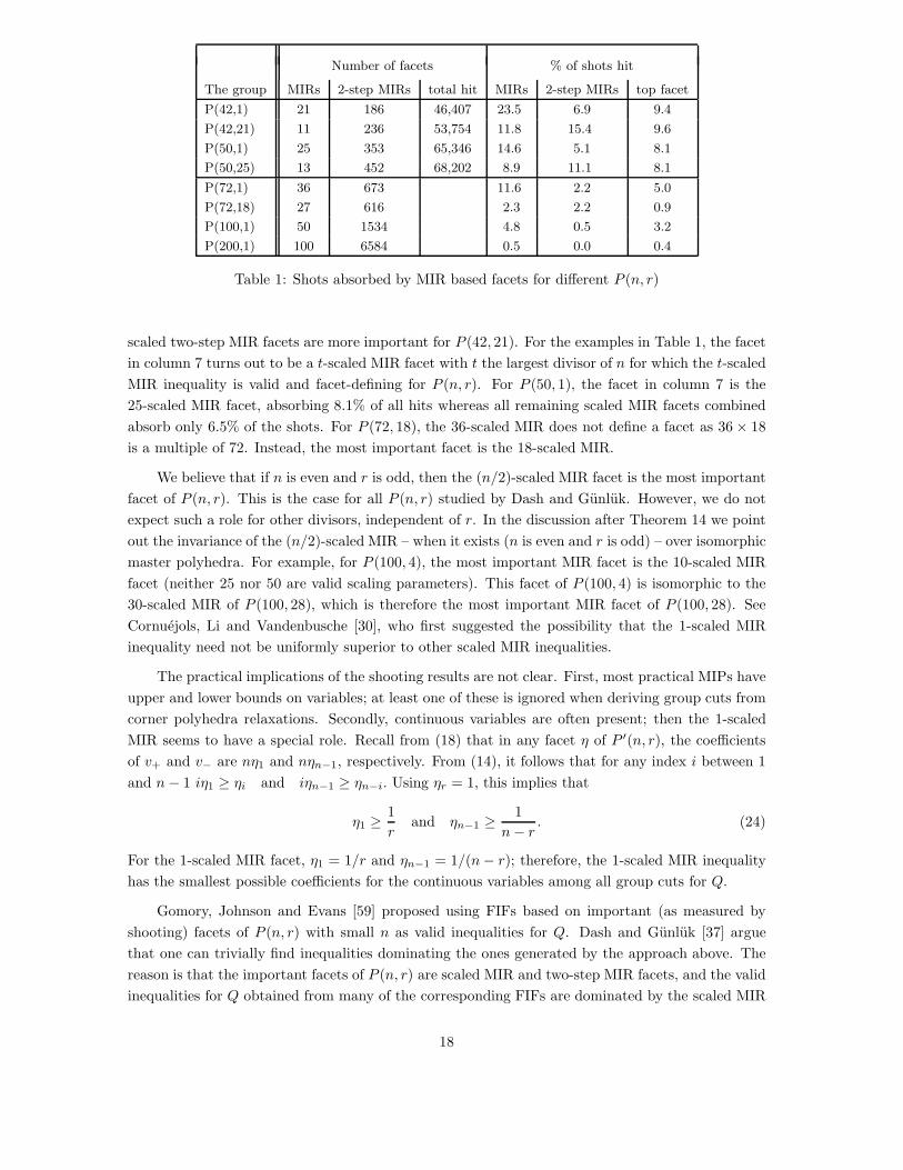
Table 1 contains results for selected master polyhedra from [37]. The second and third columns
give the number of (integrally) scaled MIR facets and two-step MIR facets. The fourth column
gives the number of distinct facets hit in 100,000 shots. The fifth, sixth, and seventh columns give,
respectively, the hit frequencies for the scaled MIR facets, the scaled two-step MIR facets, and most
frequently hit facet from these classes. For example, for P (50, 1) we see that the 378 scaled MIR and
two-step MIR facets (out of 65,346 facets) absorb almost 20% of all hits, and that a single facet from
this class absorbs 8.1% of all hits. Thus, a very few facets absorb a large fraction of all hits, and are
mostly scaled MIR and two-step MIR facets. In addition, neither class is uniformly more important
than the other. For example, for P (42, 1) the scaled MIR facets are more important, whereas the
17
Number of facets % of shots hit
The group MIRs 2-step MIRs total hit MIRs 2-step MIRs top facet
P(42,1) 21 186 46,407 23.5 6.9 9.4
P(42,21) 11 236 53,754 11.8 15.4 9.6
P(50,1) 25 353 65,346 14.6 5.1 8.1
P(50,25) 13 452 68,202 8.9 11.1 8.1
P(72,1) 36 673 11.6 2.2 5.0
P(72,18) 27 616 2.3 2.2 0.9
P(100,1) 50 1534 4.8 0.5 3.2
P(200,1) 100 6584 0.5 0.0 0.4
Table 1: Shots absorbed by MIR based facets for different P (n, r)
scaled two-step MIR facets are more important for P (42, 21). For the examples in Table 1, the facet
in column 7 turns out to be a t-scaled MIR facet with t the largest divisor of n for which the t-scaled
MIR inequality is valid and facet-defining for P (n, r). For P (50, 1), the facet in column 7 is the
25-scaled MIR facet, absorbing 8.1% of all hits whereas all remaining scaled MIR facets combined
absorb only 6.5% of the shots. For P (72, 18), the 36-scaled MIR does not define a facet as 36 × 18
is a multiple of 72. Instead, the most important facet is the 18-scaled MIR.
We believe that if n is even and r is odd, then the (n/2)-scaled MIR facet is the most important
facet of P (n, r). This is the case for all P (n, r) studied by Dash and Gunluk. However, we do not
expect such a role for other divisors, independent of r. In the discussion after Theorem 14 we point
out the invariance of the (n/2)-scaled MIR – when it exists (n is even and r is odd) – over isomorphic
master polyhedra. For example, for P (100, 4), the most important MIR facet is the 10-scaled MIR
facet (neither 25 nor 50 are valid scaling parameters). This facet of P (100, 4) is isomorphic to the
30-scaled MIR of P (100, 28), which is therefore the most important MIR facet of P (100, 28). See
Cornuejols, Li and Vandenbusche [30], who first suggested the possibility that the 1-scaled MIR
inequality need not be uniformly superior to other scaled MIR inequalities.
The practical implications of the shooting results are not clear. First, most practical MIPs have
upper and lower bounds on variables; at least one of these is ignored when deriving group cuts from
corner polyhedra relaxations. Secondly, continuous variables are often present; then the 1-scaled
MIR seems to have a special role. Recall from (18) that in any facet η of P ′(n, r), the coefficients
of v+ and v− are nη1 and nηn−1, respectively. From (14), it follows that for any index i between 1
and n − 1 iη1 ≥ ηi and iηn−1 ≥ ηn−i. Using ηr = 1, this implies that
η1 ≥1
rand ηn−1 ≥
1
n − r. (24)
For the 1-scaled MIR facet, η1 = 1/r and ηn−1 = 1/(n − r); therefore, the 1-scaled MIR inequality
has the smallest possible coefficients for the continuous variables among all group cuts for Q.
Gomory, Johnson and Evans [59] proposed using FIFs based on important (as measured by
shooting) facets of P (n, r) with small n as valid inequalities for Q. Dash and Gunluk [37] argue
that one can trivially find inequalities dominating the ones generated by the approach above. The
reason is that the important facets of P (n, r) are scaled MIR and two-step MIR facets, and the valid
inequalities for Q obtained from many of the corresponding FIFs are dominated by the scaled MIR
18

and two-step MIR inequalities for Q. See Section 3.2.
4 MIR closure
In this section, we discuss properties of the MIR closure of a polyhedral set P = v ∈ Rl, x ∈ Z
n :
Cv + Ax = b, v, x ≥ 0 with m constraints. We define the MIR closure of P as the set of points in
PLP which satisfy all MIR cuts for P , and denote it by PMIR. Nemhauser and Wolsey’s result [77]
showing the equivalence of split cuts and MIR cuts for P implies that the split closure of P – defined
as the set of points in PLP satisfying all split cuts for P – equals its MIR closure. Cook, Kannan
and Schrijver [28] showed that the split closure of P is a polyhedron. Andersen, Cornuejols and Li
[5], Vielma [86], and Dash, Gunluk and Lodi [39] give alternative proofs that the split closure of a
polyhedral set is a polyhedron. The latter proof is in terms of the MIR closure of P , and we discuss
it below. Caprara and Letchford [23] studied the separation problem for split cuts, i.e., the problem
of finding a violated split cut given a point (v∗, x∗) ∈ PLP or proving that no such cut exists. They
proved that this separation problem is NP-hard.
For a vector w, let w+ stand for maxw,0, where the maximum is taken component-wise. In
this section, we assume that A, C and b have integral components (this is without loss of generality,
as we assumed earlier that they were rational matrices). Let
Π =(λ, c+, α, α, β, β) ∈ R
m × Rl × R
n × Zn × R × Z :
c+ ≥ λC, c+ ≥ 0,
α + α ≥ λA, 1 ≥ α ≥ 0,
β + β ≤ λb, 1 ≥ β ≥ 0.
Note that for any (λ, c+, α, α, β, β) ∈ Π,
c+v + (α + α)x ≥ β + β (25)
is valid for PLP as it is a relaxation of (λC)v + (λA)x = λb. Furthermore, using the basic mixed-
integer inequality (1), we infer that
c+v + αx + βαx ≥ β(β + 1) (26)
is a valid inequality for P . We call (26) a relaxed MIR inequality derived from the base inequality
(25). (We use the notation a and β because for a fixed λ, the best choice for β equals λb, and
the best choices for components of a are 0 or fractional parts of components of λA, see the next
paragraph.) If β = 0, then the relaxed MIR inequality is trivially satisfied by all points in PLP . If
β = 1, then (26) is identical to its base inequality (25) and is satisfied by all points in PLP . Further,
(26) is a split cut for P derived from the disjunction αx ≤ β ∨ αx ≥ β + 1, and is therefore violated
by (v∗, x∗) ∈ PLP only if β < αx∗ < β + 1. This implies the following lemma.
Lemma 16 A relaxed MIR inequality (26) violated by (v∗, x∗) ∈ PLP satisfies (i) 0 < β < 1,
(ii) 0 < ∆ < 1, where ∆ = β + 1 − αx∗.
It is easy to see that the MIR inequality (5) for P is also a relaxed-MIR inequality. For a given
multiplier vector λ, let α denote λA. Further, set c+ = (λC)+, β = ⌊λb⌋ and β = λb − ⌊λb⌋. Also,
19

define α and α as follows: if αi −⌊αi⌋ < β then αi = αi − ⌊αi⌋ and αi = ⌊αi⌋, otherwise αi = 0 and
αi = ⌈αi⌉. Clearly, (λ, c+, α, α, β, β) ∈ Π and the corresponding relaxed MIR inequality (26) is the
same as the MIR inequality (5). Therefore, every split cut is also a relaxed MIR inequality.
Recall the discussion in Section 2, where we observe that the MIR inequality is the strongest
inequality of the form (3). This property and Lemma 16 are used by Dash, Gunluk and Lodi [39,
Lemma 6] to show that a point in PLP satisfies all MIR inequalities, if and only if it satisfies all
relaxed MIR inequalities. Therefore the MIR closure of P can be defined as
PMIR =(v, x) ∈ PLP : c+v + αx + βαx ≥ β(β + 1) for all (λ, c+, α, α, β, β) ∈ Π
.
Therefore, for a given point (v∗, x∗) ∈ PLP , one can test if (v∗, x∗) ∈ PMIR by solving the non-linear
integer program (MIR-SEP):
max β(β + 1) − (c+v∗ + αx∗ + βαx∗)
s.t. (λT , c+, α, α, β, β) ∈ Π.
If every solution of MIR-SEP has objective value zero or less, then (v∗, x∗) ∈ PMIR. On the other
hand, if some solution has positive objective value, it gives a violated relaxed MIR inequality. For
a point (v∗, x∗), we define the violation of a relaxed MIR inequality to be its right-hand side minus
its left-hand side evaluated at (v∗, x∗). The violation is bounded above by β(β + 1 − αx∗) which is
strictly less than 1 for a violated MIR inequality.
Observe that MIR-SEP becomes an LP if α and β are fixed to some integral values. Let φ
be a solution of MIR-SEP with objective value µ. Fix the values of α and β in MIR-SEP to the
corresponding values in φ, say αφ and βφ, respectively. The resulting LP has a basic optimal solution
φ′ with objective value ≥ µ. The LP constraints (other than the variable bounds) can be written as
AT −I
CT −I
bT −1
λ
α
c+
β
≤
≤
≥
αφ
0
βφ
.
This implies the following result.
Theorem 17 [39] If there is an MIR inequality violated by the point (v∗, x∗), then there is another
MIR inequality violated by (v∗, x∗) for which β and the components of λ, α are rational numbers with
denominator equal to a subdeterminant of [AC b].
We will now argue that Theorem 17 implies that the MIR closure of P is a polyhedron. This
argument is different from the one in [39]; there Theorem 17 is used in a different manner. Consider a
polyhedron in Rk defined by Gx+Hy ≤ b, let Φ be the maximum absolute value of subdeterminants
of [GH b]. The convex hull of its x-integral points is a polyhedron, with extreme points whose x-
coefficients have magnitude bounded by (k +1)Φ, and other coefficients have encoding size bounded
by a polynomial function of k and Φ. See Theorems 16.1 and 17.1 in [83]. By Lemma 16, every
violated relaxed-MIR inequality satisfies 0 < β < 1. Therefore, Theorem 17 implies that β can be
assumed to lie in the set B = r/s ∈ (0, 1) : r, s ∈ Z, s is a sub-determinant of [AC b]. For any
fixed β, MIR-SEP becomes a mixed-integer program; call this MIR-SEP(β). The convex hull of its
(α, β)-integral solutions is a polyhedron, say P ′(β). The set M formed by the union of the extreme
20

points of P ′(β) for β ∈ B is clearly finite. Further, the relaxed-MIR inequalities defined by this set
define the MIR closure of P . After all, if a point (v∗, x∗) is not contained in the MIR closure of P ,
by Theorem 17, it is violated by some inequality with β in B and therefore by some inequality in
M.
The above argument also implies that the relaxed-MIR cuts defining the MIR closure of P can
be derived from disjunctions contained in a bounded set; more precisely (α, β) are contained in the
set D = [−(n+l+1)Φ2, (n+l+1)Φ2]n+1, where Φ is the maximum absolute value of subdeterminants
of [AC b]. Therefore, one can derive using the equivalence of split cuts and MIR cuts that the split
closure of P equals
⋂
(c,d)∈D
conv(PLP ∩ cx ≤ d ∪ PLP ∩ cx ≥ d + 1).
Further, the vector of multipliers λ also has bounded coefficients. This result is similar to [39,
Lemma 21], where a bound on the magnitude of λ needed for non-redundant MIR cuts is given; the
latter bound is sharper as the proof in [39] does not use such general arguments.
Lemma 18 [39, Lemma 21] Assume that the coefficients in Cv + Ax = b are integers. If there is
an MIR inequality violated by the point (v∗, x∗), then there is another MIR inequality violated by
(v∗, x∗) with λi ∈ (−mΨ, mΨ), where m is the number of rows in Cv +Ax = b, and Ψ is the largest
absolute value of subdeterminants of C.
If P has no continuous variables, it is easier to show that the MIR closure of P is a polyhedron; one
can show that λ ∈ (0, 1)m. Caprara and Letchford [23, Lemma 1] show (in a different form) that
λ ∈ (−1, 1)m, when P has no continuous variables; this yields a short proof that the split closure of
P is a polyhedron.
Assume (in this paragraph) that P has no continuous variables, i.e., C = 0. The problem of
obtaining a violated Gomory-Chvatal cut be framed as a mixed-integer program, see Bockmayr and
Eisenbrand [19] and Fischetti and Lodi [47]. One can then infer, as in the discussion on the MIR
closure above, that the Chvatal closure of P is a polyhedron. Bockmayr and Eisenbrand study this
mixed-integer program and use the fact that its integral hull has polynomially many extreme points
in fixed dimension to show that the Chvatal closure of P in fixed dimension has polynomially many
facets. In fixed dimension, the number of extreme points of P ′(β) can be shown to be bounded by a
polynomial function of the encoding size of Cv+Ax = b. If one can show that M is the union of P ′(β)
for polynomially many choices of β, then one could give a positive answer to Eisenbrand’s question
[43]: Does the MIR (or split) closure of P have polynomially many facets in fixed dimension? Dash,
Gunluk and Lodi show that the separation problem for MIR cuts can be framed as a mixed-integer
program (see the discussion below). Unfortunately, the number of variables in their separation
MIP depends on the encoding size of [AC b] and one cannot use the technique of Bockmayr and
Eisenbrand to give a positive answer to Eisenbrand’s question.
We next describe the approximate MIR separation model in [39] obtained by approximately
linearizing the product β(β + 1− αx∗) in the objective function of MIR-SEP. Define a new variable
∆ that stands for (β +1− αx). Let β ≤ β be an approximation of β which is representable over some
E = ǫk : k ∈ K. Let a number δ be representable over E if δ =∑
k∈K ǫk for some K ⊆ K. One can
write β as∑
k∈K ǫkπk using binary variables πk, and approximate β∆ by β∆. This last term can
21

be written as∑
k∈K ǫkπk∆. This results in the following approximate MIP model APPX-MIR-SEP
for the separation of the most violated MIR inequality:
max∑
k∈K
ǫk∆k − (c+v∗ + αx∗) (27)
s.t. (λ, c+, α, α, β, β) ∈ Π (28)
β ≥∑
k∈K
ǫkπk (29)
∆ = (β + 1) − αx∗ (30)
∆k ≤ ∆ ∀k ∈ K (31)
∆k ≤ πk ∀k ∈ K (32)
π ∈ 0, 1|K| (33)
Let zsep and zapx−sep denote the optimal values of MIR-SEP and APPX-MIR-SEP, respectively.
For any integral solution of APPX-MIR-SEP, (λ, c+, α, α, β, β) ∈ Π and
∑
k∈K
ǫk∆k ≤∑
k∈K
ǫk∆πk ≤ β∆,
implying that zsep ≥ zapx−sep. In other words, if the approximate separation problem finds a
solution with objective function value zapx−sep > 0, the corresponding MIR cut is violated by at
least as much. In the computational experiments of Dash, Gunluk and Lodi with APPX-MIR-SEP,
they use E = 2−k : k = 1, . . . , k for some small number k (between 5 and 7). They prove that with
this choice of E , APPX-MIR-SEP yields a violated MIR cut provided that there is an MIR cut with
a “large enough” violation. More precisely, they prove [39, Theorem 8] that zapx−sep > zsep − 2−k.
If the relaxed-MIR inequality I with maximum violation has a value of β which is representable
over E , one can choose π ∈ 0, 1k such that β =∑
k∈K ǫkπk. Set ∆ = β + 1 − αx∗. Set ∆k = 0 if
πk = 0, and ∆k = ∆ if πk = 1. Then ∆k = πk∆ for all k ∈ K, and β∆ =∑
k∈K ǫk∆k. Therefore, the
relaxed-MIR inequality I yields an optimal solution of APPX-MIR-SEP whose objective function
value equals the violation of the I. In other words, zsep = zapx−sep. Theorem 17 implies that
β in a violated MIR cut can be assumed to be a rational number with a denominator equal to a
subdeterminant of [AC b]. This implies the following result.
Theorem 19 [39] Let Φ be the least common multiple of all subdeterminants of [AC b], K =
1, . . . , logΦ, and E = ǫk = 2k/Φ, ∀k ∈ K. Then APPX-MIR-SEP is an exact model for finding
violated MIR cuts.
Caprara and Letchford [23], and more recently, Balas and Saxena [16], present optimization
models for finding a violated split cut for P . In both papers, the authors use two sets of multipliers
that guarantee that the split cut is valid for both sides of the disjunction; see equations (8)-(13)
in [23] and equation (SP) in [16]. It is argued in [39] that the separation model in Caprara and
Letchford (equations (8)-(13)) actually finds the most violated MIR cut (the objective function
22

equals four times the objective function of MIR-SEP). In other words, an optimal solution of MIR-
SEP is also optimal for the Caprara-Letchford model and vice-versa. Similarly, the Balas-Saxena
model (equation (2.1) or (PMILP) in [16]) is equivalent to MIR-SEP, and has the same objective
function. Consequently, the models in [23] and [16] are also equivalent to each other.
Caprara and Letchford do not perform any computational tests with their model. As for Balas
and Saxena, instead of bounding β by β and linearizing β∆ as in [39], they fix the term corresponding
to 1 − β in their model to specific values between 0 and 1/2, and for each value, solve an MIP to
obtain a violated split cut. We will discuss some of the computational results in [39] and [16] in the
next section.
5 Computational issues
Balas, Ceria, Cornuejols and Natraj [14] showed that GMI cuts (MIR cuts with simplex tableau
rows as base inequalities), when added in rounds (all violated GMI cuts for the current optimal
tableau are added simultaneously), are very useful in solving the general mixed-integer programs in
MIPLIB 3.0. Bixby et. al. [18] extended this observation to larger problem sets, and performed
additional experiments confirming the usefulness of GMI cuts relative to other cuts in the CPLEX
solver. Marchand and Wolsey [72] proposed a different, effective way of generating MIR inequalities;
their heuristic aggregates constraints of the original formulation to obtain base inequalities which
are different from simplex tableau rows. Despite their effectiveness, GMI cuts often cause numerical
difficulties, and this aspect limits their use. In some cases, simple implementations yield invalid cuts
[73]; in other cases, adding too many GMI cuts makes the resulting LP hard to solve. The issue of
invalid cuts is addressed in a recent paper by Cook et. al. [26] who generate provably valid GMI cuts
with negligible reduction in performance (as measured by computing time and quality of bounds).
After Gomory [55] introduced group relaxations in 1965, White [87] and Shapiro [84] showed
that for a number of small IPs, group relaxations yielded strong bounds on optimal values. For
12 of the 14 problems in the latter paper where the IP optimal is known and is different from the
LP relaxation value, the group relaxation bound equals the optimal value. Gorry, Northup and
Shapiro [60] performed a detailed study of a group relaxation based branch-and-bound algorithm,
and solved problems with up to 176 rows and 2385 columns. In the above papers, group relaxations
were solved via dynamic programming algorithms. See Salkin [82, Chapter 9] for a discussion on
early computational work on this topic. In general it is NP-hard to solve the group relaxation
problem or, equivalently, to optimize over an arbitrary corner polyhedron [69] (or strengthened
corner polyhedra [48]). In a recent computational study, Fischetti and Monaci [48] optimize over
the corner polyhedra (also strengthened corner polyhedra) associated with optimal vertices of LP
relaxations of some MIPLIB 3.0 and MIPLIB 2003 instances by solving MIPs and show that the
average integrality gap closed is 23.61% (34.48%) as opposed to 25.32% with GMI cuts. The gap
closed using corner polyhedra relaxations is worse than that with GMI cuts; this is because throwing
away the non-active bounds on variables often results in weak bounds on optimum values for MIPLIB
instances, especially those which have binary variables.
Two interesting directions of research extending the above work consist of (a) generating valid
inequalities other than MIR cuts – especially group cuts – from the same base inequalities, and (b)
aggregating constraints of the original formulation to obtain base inequalities different from simplex
23

tableau rows or those generated by Marchand and Wolsey. The difference between recent work on
(a) and earlier work in the previous paragraph is that the corner polyhedron is used to generate
cutting planes, rather than as a relaxation by itself.
For the mixed-integer knapsack polyhedron, Atamturk [9] developed valid inequalities (via lift-
ing) which use upper and lower bounds on variables, unlike the MIR cut in (5) which uses only
one of the bounds. For a collection of randomly generated multiple knapsack instances [10], his
inequalities along with MIR cuts close a significantly larger fraction of the integrality gap than MIR
cuts alone. He uses scaled constraints of the original formulation as base inequalities. Fischetti and
Saturni [49] and Dash, Goycoolea and Gunluk [35] study the effectiveness of group cuts derived from
simplex tableau rows relative to GMI cuts. The first paper contains a study of group cuts derived via
interpolation; violated cuts of this type are obtained by solving an LP. The second paper presents
a heuristic to generate violated two-step MIR inequalities, and shows that they are useful for the
randomly generated instances of Atamturk. For the unbounded instances (variables are nonnegative
and not bounded above) in Atamturk’s data set, two-step MIR inequalities derived from rows of
the initial optimal simplex tableau combined with GMI cuts (derived from the same tableau rows)
close 78.65% of the integrality gap, whereas GMI cuts alone close only 56.25% of the integrality
gap. For these instances, two-step MIR inequalities seem to be as effective as the lifted knapsack
cuts of Atamturk, and more effective than K-cuts [30]. Fischetti and Saturni show that K-cuts
for K = 1, . . . , 50 (or 1-50 scaled GMI cuts) close 75.99% of the integrality gap. Interestingly, the
integrality gap closed via (strengthened or otherwise) corner polyhedra relaxations [48] is 79.43%,
which is only slightly better than the gap closed using two-step MIR inequalities. These experiments
suggest that the shooting experiments discussed earlier yield useful information for problems which
resemble master cyclic group polyhedra in that the integer variables can take values from a large in-
terval, and the constraints have general (not 0-1) coefficients. For the bounded Atamturk instances,
we note that the lifted knapsack cuts are more (about 5-6%) effective in closing the integrality gap
than two-step MIR inequalities.
The authors in [35] observe that for the problems in MIPLIB 3.0, the gap closed by one round of
two-step MIR cuts + GMI cuts is essentially the same as that closed by one round of GMI cuts alone.
Interpolated group cuts, and 1-50 scaled GMI cuts also seem to behave similarly [49]. Motivated by
this observation, Dash and Gunluk [38] demonstrate that for a collection of practical instances (from
MIPLIB 3.0, MIPLIB 2003, MILPLib [75], and instances from [71]), after GMI cuts derived from the
initial optimal tableau rows are added, the solution of the resulting relaxation satisfies all non-GMI
group cuts derived from the initial tableau rows for 35% of the instances. In other words, additional
group cuts beyond the GMI cut derived from the initial optimal tableau rows are not useful at all
for these instances. On the other hand, for 82% of the remaining instances (which potentially have
violated group cuts), one can find violated two-step MIR inequalities. Thus, unlike the Atamturk
instances, group cuts from single tableau rows do not seem to be very useful for the above instances.
However, two-step MIR inequalities seem to be important relative to other group cuts. Fukasawa
and Goycoolea [50] extend the above experiments for MIPLIB instances to show that no other valid
inequalities derived from the mixed-integer knapsacks defined by initial optimal tableau rows and
bounds on variables improve the integrality gap by a significant margin. The above experiments
suggest that for MIPLIB instances, in order to obtain cutting planes which improve the integrality
gap closed by GMI cuts, it is important to use information from multiple constraints simultaneously.
Some recent computational work in this direction can be found in Espinoza [45].
24

Bonami and Minoux [21] approximately optimize over the lift-and-project closure of 0-1 mixed
integer programs via the equivalence of optimization and separation; in this context the separa-
tion problem can be framed as a linear program. Lift-and-project cuts are split cuts derived from
disjunctions of the form xi ≤ 0 ∨ xi ≥ 1 for some integral variable xi. Balas and Perregard [15] pro-
posed a method to generate strengthened lift-and-project cuts from simplex tableau rows, and their
method and some variants were implemented by Balas and Bonami [13] with encouraging results.
Independently, Fischetti and Lodi [47] show that for many practical MIPs, one can separate points
from the Chvatal closure of pure integer programs in reasonable time by formulating the separation
problem as an MIP and solving it with a general MIP solver. They apply their separation algo-
rithm to approximately optimize over the Chvatal closures of MIPLIB instances and obtain tight
bounds on optimal solution values for many instances. Bonami et. al. [20] extend the definition of
Gomory-Chvatal cuts to mixed integer programs (projected Gomory-Chvatal cuts) and use a similar
MIP based separation procedure to obtain bounds for mixed-integer programs in MIPLIB 3.0.
Optimizing over the split closure of MIPs should lead to stronger bounds than in the papers
above. Balas and Saxena [16] approximately optimize over the split closure of MIPLIB instances to
obtain strong bounds on their optimal values, and so do Dash, Gunluk and Lodi [39], who combine
APPX-MIR-SEP with some heuristics to find violated MIR cuts. In MIPLIB 3.0, 62 of the 65
instances have a non-zero integrality gap, other than dsbmip, enigma and noswot. Balas and Saxena
show that for these instances (other than arki001 where they use cuts which potentially have MIR
rank 2), at least 71.3% of the integrality gap can be closed by optimizing over the split closure (the
computation time is quite high though). For these 62 instances, Dash, Gunluk and Lodi show that
at least 59.3% of the integrality gap can be closed in one hour of computation time; a round of GMI
cuts closes only 28.4% of the integrality gap. For the 21 pure IPs, the gaps closed by Dash, Gunluk
and Lodi, Fischetti and Lodi (GC cuts), Balas and Saxena, and GMI cuts are on the average 59.2%,
56.5%, 76.0% and 29.8%, respectively. For the remaining 41 MIPs, the corresponding numbers
(with projected-GC cuts instead of GC cuts) are, respectively, 59.3, 28.8, 68.9, and 27.7. Note that
in Bonami et. al. [20], the bounds for projected-GC cuts are obtained with only 20 minutes of
computation, whereas the bounds with GC cuts in [47] are obtained after 3 hours of computation,
on the average.
6 Proof complexity
If NP 6= coNP , then it cannot be true that for arbitrary Ax ≤ b without 0-1 solutions, there is
a polynomial-size (in the encoding size of A, b) certificate of the absence of 0-1 solutions. We next
discuss a recent result in [33] which proves the existence of a family of inequality systems without
0-1 solutions for which MIR cutting-plane proofs of 0-1 infeasibility have exponential length.
A boolean circuit can be viewed as a description of the elementary steps in an algorithm via
a directed acyclic graph with three types of nodes: input nodes – nodes with no incoming arcs,
a single output node – the only node with no outgoing arcs, and computation nodes (also called
gates), each of which is labelled by one of the boolean functions ∧,∨, and ¬. For nodes i and j, an
arc ij means that the value computed at i is used as an input to the gate at node j. A computation
is represented by placing 0-1 values on the input gates, and then recursively applying the gates to
inputs on incoming arcs, till the function at the output node is evaluated. A function f : Rn → R is
25

monotone if for x, y in Rn, x ≤ y implies f(x) ≤ f(y). Monotone operations are monotone functions
with one or two inputs; some examples are
tx, r + x, x + y, ⌊x⌋, thr(x, 0)
where t is a non-negative constant, x and y are real variables, and r is a real constant; thr(x, 0) is a
threshold function which returns 0, if x < 0, and 1 otherwise. The functions ∧ and ∨ are monotone
operations over the domain 0, 1. The function f(x, y) = x−y, where x, y ∈ R, is not monotone. A
monotone boolean circuit uses only ∧ gates and ∨ gates; a monotone real circuit is one with arbitary
monotone operations as gates.
Consider CLIQUEk,n (say k is a fixed function of n), the function which takes as input n-node
graphs (represented by incidence vectors of their edges) and returns 1 if the graph has a clique of size
k or more, and 0 otherwise. This function is monotone, as adding edges to a graph (changing some
zeros to ones in the incidence vector) causes the maximum clique size to increase. Every monotone
boolean function can be computed by a monotone boolean circuit. Razborov [80] showed that any
monotone boolean circuit solving CLIQUEk,n (for appropriate k) has a super-polynomial number
of gates, and Alon and Boppana [4] strengthened his bound to an exponential lower bound. Pudlak
[78], and independently, Cook and Haken [27], proved that the above bounds hold for monotone real
circuits.
Theorem 20 [78] Let Cn be a monotone real circuit which takes as input graphs on n nodes (given
as incidence vectors of edges), and returns 1 if the input graph contains a clique of size k = ⌊n2/3⌋,
and 0 if the graph contains a coloring of size k − 1 (and returns 0 or 1 for all other graphs). Then
|Cn| ≥ 2Ω((n/ log n)1/3).
Pudlak [78] presented a set of linear inequalities I related to the problem of Theorem 20 such
that if I has a 0-1 solution, then there is a graph on n nodes which has both a clique of size
k and a coloring of size k − 1. He proved that given a Gomory-Chvatal cutting plane proof P
with L cuts which proves that I has no 0-1 solution, one can construct a monotone real circuit
with O(poly(size(P))) gates solving CLIQUEk,n. Therefore L is exponential in n. Pudlak used
the following properties of Gomory-Chvatal cuts in mapping short cutting-plane proofs to small
monotone real circuits:
(1) If gx + hy ≤ d is a Gomory-Chvatal cut for Ax + By ≤ c, then for any 0-1 vector y, gx ≤ d− hy
is a Gomory-Chvatal cut for Ax ≤ c − By;
(2) if gx + hy ≤ d is a Gomory-Chvatal cut for Ax ≤ e, By ≤ f , then there are numbers r and s
such that gx ≤ r is a Gomory-Chvatal cut for Ax ≤ e, and hy ≤ s is a Gomory-Chvatal cut for
By ≤ e, and r + s ≤ d.
(3) The number r (or s) can be computed from A, e (or B, f) with polynomially many monotone
operations.
Property (1) is easy to prove for all integer vectors y. Consider property (2). As gx + hy ≤ d
is a Gomory-Chvatal cut for Ax ≤ e, By ≤ f , we can assume that g, h, d are integral and there
are multiplier vectors λ, µ ≥ 0 such that g = λA, h = µB, d = ⌊λe + µf⌋. Clearly, gx ≤ ⌊λe⌋ is a
Gomory-Chvatal cut for Ax ≤ e, and so is hy ≤ ⌊µf⌋, and ⌊λe⌋ + ⌊µf⌋ ≤ ⌊λe + µf⌋. Property (3)
also follows from this; the number ⌊λe⌋ can be computed from e via polynomially many monotone
operations (the coefficients of λ are treated as non-negative constants).
26
In general, for a class of cutting planes C, if we can prove properties (1)-(3) in the previous
paragraph for C, then given a C-proof of the fact that Pudlak’s inequality system I has no 0-1
solution, we can construct a monotone real circuit solving CLIQUEk,n with polynomially many
gates (in the size of the C-proof). This would yield an exponential worst-case lower bound on the
size of C-proofs certifying that I has no 0-1 solution (of course, additional details have to be verified).
In general, for many classes of cutting planes properties (1) and (2) hold, e.g., the matrix cuts of
Lovasz and Schrijver (cuts based on the N and N+ operators; see [79], [32]. Property (3) is often
hard to prove, and is not known to hold for matrix cuts. We prove in [33] that slight variants of
properties (2) and (3) hold for MIR cuts, and thereby obtain an exponential worst-case lower bound
on the complexity of MIR cuts. We state this result below. For completeness, we explicitly give the
inequality system I.
Let k = ⌊n2/3⌋. Let z be a vector of n(n − 1)/2 0-1 variables, such that every 0-1 assignment
to z corresponds to the incidence vector of a graph on n nodes (assume nodes are numbered from
1, . . . , n). Let x be the 0-1 vector of variables (xi | i = 1, . . . , n) and let y be the 0-1 vector of variables
(yij | i = 1, . . . , n, j = 1, . . . , k − 1). Consider the inequalities
∑
i
xi ≥ k, (34)
xi + xj ≤ 1 + zij , ∀ i, j ∈ N, with i < j, (35)
k−1∑
j=1
yij = 1, ∀i ∈ N, (36)
yis + yjs ≤ 2 − zij , ∀ i, j ∈ N with i < j, and ∀s ∈ 1, . . . , k − 1. (37)
Then, in any 0-1 solution of the above inequalities, the set of nodes i |xi = 1 forms a clique of size
k or more, and for all j ∈ 1, . . . , k − 1, the set i | yij = 1 is a stable set. Thus, the variables yij
define a mapping of nodes in a graph to k − 1 colors in a proper colouring. Let Ax + Cz ≤ e stand
for the inequalities (34) and (35), along with the bounds 0 ≤ x ≤ 1. Let By + Dz ≤ f stand for the
inequalities (36) and (37), along with the bounds 0 ≤ y ≤ 1 and 0 ≤ z ≤ 1. Then any 0-1 solution
of Ax + Cz ≤ e and By + Dz ≤ f corresponds to a graph which has both a clique of size k, and
a coloring of size k − 1. Clearly, no such 0-1 solution exists. Note that the above inequalities have
O(n3) variables and constraints.
Theorem 21 [33] Every MIR cutting-plane proof of 0x + 0y + 0z ≤ −1 from Ax + Cz ≤ e and
By + Dz ≤ f has exponential length.
Many families of inequalities are either special cases of MIR cuts (e.g., Gomory-Chvatal cuts, lift-
and-project cuts), or can be obtained as rank k MIR cuts for some fixed number k. For example,
the two-step MIR inequalities have MIR rank 2 or less. Therefore, one trivially obtains exponential
worst-case lower bounds for the complexity of cutting plane proofs for all such families of cutting
planes.
The technique of deriving a polynomial size monotone circuit from a proof of infeasibility is
called monotone interpolation, and was proposed by Krajıcek [65, 66] to establish lower bounds on
the lengths of proofs in different proof systems. Razborov [81], and Bonet, Pitassi, and Raz [22],
first used this idea to prove exponential lower bounds for some proof systems.
27
Acknowledgements
I would like to thank Vasek Chvatal for inviting to me present the lectures at the NATO
Summer School on which this survey is based. I would also like to thank Oktay Gunluk for numerous
productive discussions on corner polyhedra.
References
[1] http://miplib.zib.de.
[2] T. Achterberg, T. Kock, and A. Martin, MIPLIB 2003. Operations Research Letters 34(4)
361–372, 2006.
[3] A. Agra and M. F. Constantino, Description of 2-integer continuous knapsack polyhedra, to
appear in Discrete Optimization (2006).
[4] N. Alon and R. Boppana, The monotone circuit complexity of Boolean functions, Combinatorica
7 1–22 (1987).
[5] K. Andersen, G. Cornuejols and Y. Li, Split Closure and Intersection Cuts, Mathematical
Programming Series A 102 (2005), 457-493.
[6] K. Andersen, Q. Louveaux, R. Weismantel and L. A. Wolsey, Inequalities from Two Rows of a
Simplex Tableau, IPCO 2007, 1–15.
[7] D. Applegate, R. Bixby, V. Chvatal, and W. Cook, TSP cuts which do not conform to the tem-
plate paradigm, in M. Junger and D. Naddef, eds., Computational Combinatorial Optimization,
Springer, 2001.
[8] J. Araoz, R.E. Gomory, E.L. Johnson, and L. Evans, Cyclic group and knapsack facets, Math-
ematical Programming 96 377–408 (2003).
[9] A. Atamturk, On the Facets of the Mixed-Integer Knapsack Polyhedron, Mathematical Pro-
gramming 98 145–175 (2003).
[10] http://ieor.berkeley.edu/∼atamturk.data.
[11] A. Atamturk and D. Rajan, Valid Inequalities for Mixed-Integer Knapsack from Two-Integer
Variable Restrictions, IEOR, University of California–Berkeley, Technical report BCOL.04.02,
(2004).
[12] E. Balas, Disjunctive programming, Annals of Discrete Mathematics 5 (1979), 3–51.
[13] E. Balas and P. Bonami, Generating lift-and-project cuts from the LP simplex tableau: open
source implementation and testing of new variants. Mathematical PRogramming Computation
1 165–200, 2010.
[14] E. Balas, S. Ceria, G. Cornuejols, G. Natraj, Gomory cuts revisited, Operations Research Letters
19 1–9 (1996).
28

[15] E. Balas and M. Perregaard, A precise correspondence between lift-and-project cuts, simple dis-
junctive cuts, and mixed integer Gomory cuts for 0-1 programming, Mathematical Programming
94 221–245 (2003).
[16] E. Balas and A. Saxena, Optimizing over the split closure. Mathematical Programming 113
219–240, 2008.
[17] R. E. Bixby, S. Ceria, C. M. McZeal, M. W. P. Savelsbergh. An updated mixed integer pro-
gramming library: MIPLIB 3.0. Optima 58 12–15 (1998).
[18] R. E. Bixby, M. Fenelon, Z. Gu, E. Rothberg, and R. Wunderling. MIP: Theory and practice –
closing the gap. In M. J. D. Powell and S. Scholtes, eds., System Modelling and Optimization:
Methods, Theory, and Applications, pages 19–49. Kluwer Academic Publishers, 2000.
[19] A. Bockmayr and F. Eisenbrand, Cutting planes and the elementary closure in fixed dimension,
Mathematics of Operations Research 26 304–312 (2001).
[20] P. Bonami, G. Cornuejols, S. Dash, M. Fischetti, and A. Lodi, Projected Chvatal-Gomory cuts
for mixed integer linear programs, Mathematical Programming 113 (2008) 241–257.
[21] P. Bonami and M. Minoux, Using rank-1 lift-and-project closures to generate cuts for 0-1 MIPs,
a computational investigation, Discrete Optimization 2 (2005), 288–307.
[22] M. Bonet, T. Pitassi, and R. Raz, Lower bounds for cutting planes proofs with small coefficients,
Journal of Symbolic Logic 62 708–728 (1997).
[23] A. Caprara and A. N. Letchford, On the separation of split cuts and related inequalities, Math-
ematical Programming 94 279–294 (2003).
[24] V. Chvatal, Edmonds polytopes and a hierarchy of combinatorial problems, Discrete Mathe-
matics 4 305–337 (1973).
[25] M. Conforti and L. A. Wolsey, Compact formulations as a union of polyhedra, Mathematical
Programming 114 277–289 (2008).
[26] W. Cook, S. Dash, R. Fukasawa, and M. Goycoolea, Numerically accurate Gomory mixed-
integer cuts, Informs Journal On Computing 21 641–649 (2009).
[27] S. A. Cook and A. Haken, An exponential lower bound for the size of monotone real circuits,
Journal of Computer and System Sciences 58 326–335 (1999).
[28] W. J. Cook, R. Kannan, and A. Schrijver, Chvatal closures for mixed integer programming
problems, Mathematical Programming 47 155–174 (1990).
[29] G. Cornuejols, Revival of the Gomory Cuts in the 1990s, State-of-the-Art and Recent Advances
in Integer Programming, 2005.
[30] G. Cornuejols, Y. Li and D. Vandenbussche, K-Cuts: A Variation of Gomory Mixed Integer
Cuts from the LP Tableau, INFORMS Journal on Computing 15 385–396 (2003).
[31] G. Cornuejols and F. Margot, On the Facets of Mixed Integer Programs with Two Integer
Variables and Two Constraints, Mathematical Programming, to appear.
29

[32] S. Dash, An exponential lower bound on the length of some classes of branch-and-cut proofs,
Mathematics of Operations Research 30(3) (2005) 678–700.
[33] S. Dash, On the complexity of cutting plane proofs using split cuts, Operations Research Letters
38 109–114 (2010).
[34] S. Dash, R. Fukasawa, and O. Gunluk. On a Generalization of the Master Cyclic Group Poly-
hedron, Mathematical Programming, to appear; DOI 10.1007/s10107-008-0252-7, 2008.
[35] S. Dash, M. Goycoolea, and O. Gunluk, Two step MIR inequalities for mixed-integer programs,
Informs Journal On Computing 22 236–249 (2010).
[36] S. Dash and O. Gunluk, Valid inequalities based on simple mixed-integer sets, Mathematical
Programming 105 29–53 (2006).
[37] S. Dash and O. Gunluk, Valid inequalities based on the interpolation procedure, Mathematical
Programming 106 111–136 (2006).
[38] S. Dash and O. Gunluk, On the strength of Gomory mixed-integer cuts as group cuts, Mathe-
matical Programming 115 387–407 (2008).
[39] S. Dash, O. Gunluk and A. Lodi, MIR closures of polyhedral sets, Mathematical Programming
121 33–60 (2010).
[40] S. S. Dey and J. P. Richard, Two Families of Facets for the Two-Dimensional Mixed Integer
Infinite Group Problem, Mathematics of Operations Research 33 140–166 (2008).
[41] S. S. Dey and J. P. Richard, Relations Between Facets of Low- and High-Dimensional Group
Problems, Mathematical Programming 123 285–313 (2010).
[42] F. Eisenbrand, On the membership problem for the elementary closure of a polyhedron, Com-
binatorica 19 (1999), 297–300.
[43] F. Eisenbrand, Split cuts and the stable set polytope of quasi-line graphs, Presentation at the
IMA special workshop: mixed-integer programming, July ’05, IMA, Minnesota (2005).
[44] D. Espinoza, Ph.D. Thesis, Industrial and Systems Engineering, Georgia Institute of Technology,
2006.
[45] D. Espinoza, Computing with multi-row group cuts, in Proceedings of IPCO 2008 (A. Lodi,
A. Panconesi, G. Rinaldi, eds.), Lecture Notes in Computer Science 5035, pp. 214–224, 2008.
[46] L. Evans, Cyclic Groups and Knapsack Facets with Applications to Cutting Planes, Ph.D.
Thesis, Georgia Institute of Technology, Atlanta, Georgia, 2002.
[47] M. Fischetti and A. Lodi, Optimizing over the first Chvatal closure, Mathematical Programming
110 3–20 (2007).
[48] M. Fischetti and M. Monaci, How tight is the corner relaxation?, Discrete Optimization 5
262–269 (2008).
[49] M. Fischetti, C. Saturni, Mixed integer cuts from cyclic groups, Mathematical Programming
109 27–53 (2007).
30

[50] R. Fukasawa and M. Goycoolea, On the exact separation of mixed-integer knapsack cuts, in
Proceedings of IPCO 2007 (M. Fischetti, D. P. Williamson, eds.), Lecture Notes in Computer
Science 4513, pp.225–239, 2007.
[51] A. M. Geoffrion and G. W. Graves, Multicommodity distribution system design by Benders
Decomposition, Management Science 20 822–844 (1974).
[52] A. M. Geoffrion, A guided tour of recent practical advances in integer linear programming,
OMEGA 4(1) 49–57 (1976).
[53] R. E. Gomory, Outline of an algorithm for integer solutions to linear programs, Bulletin of the
American Mathematical Society 64 275–278 (1958).
[54] R. E. Gomory, An algorithm for the mixed integer problem, RM-2597, The Rand Corporation,
1960.
[55] R. E. Gomory, On the relation between integer and noninteger solutions to linear programs,
Proceedings of the National Academy of Sciences 53(2) 260–265 (1965).
[56] R.E. Gomory, Some polyhedra related to combinatorial problems, Journal of Linear Algebra
and its Applications 2 451–558 (1969).
[57] R.E. Gomory and E. Johnson, Some continuous functions related to corner polyhedra I, Math-
ematical Programming 3 23–85 (1972).
[58] R.E. Gomory and E. Johnson, Some continuous functions related to corner polyhedra II, Math-
ematical Programming 3 359–389 (1972).
[59] R.E. Gomory, E.L. Johnson, and L. Evans, Corner Polyhedra and their connection with cutting
planes, Mathematical Programming 96 321–339 (2003).
[60] G. Gorry, W. Northup, and J. Shapiro, Computational experience with a group theoretic integer
programming algorithm, Mathematical Programming 4 171–192 (1973).
[61] O. Gunluk, and Y. Pochet, Mixing Mixed-Integer Inequalities, Mathematical Programming 90
429–457 (2001).
[62] B. Hunsaker and C. Tovey, Separation of rank 1 Chvatal-Gomory inequalities, presentation at
the INFORMS Computing Society conference, Annapolis, MD (2005).
[63] ILOG Cplex 9.0: User’s Manual and Reference Manual, ILOG, S.A., http://www.ilog.com/,
2005.
[64] K. Kianfar and Y. Fathi, Generalized mixed integer rounding inequalities: facets for infinite
group polyhedra, Mathematical Programming 120 313–346 (2009).
[65] J. Krajıcek, Lower bounds to the size of constant-depth propositional proofs, Journal of Sym-
bolic Logic 59 73–86 (1994).
[66] J. Krajıcek, Interpolation theorems, lower bounds for proof systems and independence results
for bounded arithmetic, Journal of Symbolic Logic 62 457–486 (1997).
31

[67] H.W. Kuhn, Discussion, in Proceedings of the IBM Scientific Computing Symposium on Combi-
natorial Problems: March 16–18, 1964, L. Robinson, ed., IBM, White Plains, New York (1966),
pp. 118–121.
[68] H.W. Kuhn, On the origin of the Hungarian Method, in History of mathematical programming:
a collection of personal reminiscences.
[69] A. N. Letchford, Binary clutter inequalities for integer programs, Mathematical Programming
98 201–221 (2003).
[70] A. N. Letchford and A. Lodi, Strengthening Chvatal-Gomory cuts and Gomory fractional cuts,
Operations Research Letters 30(2) 74–82 (2002).
[71] http://www.or.deis.unibo.it/research pages/ORinstances/MIPs.html.
[72] H. Marchand and L. A. Wolsey, Aggregation and mixed integer rounding to solve MIPs, Oper-
ations Research 49, 363–371 (2001).
[73] F. Margot, Testing Cut Generators for Mixed-Integer Linear Programming, Mathematical Pro-
gramming Computation 1 69–95 (2009).
[74] L. Miller, Y. Li, and J. P. Richard, New inequalities for finite and infinite group problems from
approximate lifting, Naval Research Logistics 55 172–191 (2008).
[75] H. Mittelmann, MILPLib, http://plato.asu.edu/topics/testcases.html.
[76] G.L. Nemhauser and L.A. Wolsey, Integer and Combinatorial Optimization, Wiley, New York
(1988).
[77] G. Nemhauser and L. A. Wolsey, A recursive procedure to generate all cuts for 0-1 mixed integer
programs, Mathematical Programming 46, 379–390 (1990).
[78] P. Pudlak, Lower bounds for resolution and cutting plane proofs and monotone computations,
Journal of Symbolic Logic 62 981–998 (1997).
[79] P. Pudlak, On the complexity of propositional calculus, Sets and Proofs, Invited papers from
Logic Colloquium 1997, Cambridge University Press, Cambridge, UK, 1999, pp. 197–218.
[80] A. A. Razborov, Lower bounds for the monotone complexity of some boolean functions, Dok-
ladi Akademii Nauk SSSR 281 798–801 (1985) (in Russian). English translation in: Soviet
Mathematics - Doklady 31 354–357 (1985).
[81] A. A. Razborov, Unprovability of lower bounds on the circuit size in certain fragments of
bounded arithmetic, Izvestiiya of the RAN 59 201–224 (1995).
[82] H. M. Salkin, Integer Programming, Addison-Wesley, 1975.
[83] A. Schrijver, Theory of Linear and Integer Programming, Wiley, Chichester (1986).
[84] J. Shapiro, Group theoretic algorithms for the integer programming problem – II: extension to
a general algorithm, Operations Research 16 928–947 (1968).
[85] E. Uchoa, Robust Branch-and-Cut-and-Price for the CMST Problem and Extended Capacity
Cuts, presentation at the MIP 2005 Workshop, IMA, Minneapolis, MN (2005).
32

[86] J. P. Vielma, A Constructive Characterization of the Split Closure of a Mixed Integer Linear
Program, Operations Research Letters 35 (2007), 29–35.
[87] W. White, On a group theoretic approach to linear integer programming, Operations Research
Center Report 66-27, University of California, Berkeley, 1966.
[88] L.A. Wolsey, Integer Programming, Wiley, New York (1998).
[89] XPRESS-MP, Extended Modelling and Optimisation Subroutine Library, Reference Manual,
Release 17, Dash Associates, Blisworth House, Blisworth, Northants NN73BX, UK (2006).
33
Recommended