
by C. Leslie, E. Eskin, J. Weston, W.S. Noble
Mismatch String Kernels for SVM
Protein Classification
by C. Leslie, E. Eskin, J. Weston, W.S. Noble
Athina Spiliopoulou
Morfoula Fragopoulou
Ioannis Konstas

Outline� Definitions & Background
� Proteins
� Remote Homology Detection
� SVMs
� Insides of the algorithm
� Feature mapping� Feature mapping
� Mismatch tree data structure
� Mismatch tree traversal
� Computational Efficiency
� Experiments
� Discussion

Proteins
Primary structure: amino acid sequence
Secondary Structure
3D Structure
� The same amino-acid sequence almost always folds
into the same 3D structure

Homologues, Remote Homologues
� Amino acid sequences subject to mutation
� Structures serving important biological function
highly conserved
� Homologues: share the same ancestor + sequence
similarity > 30% similarity > 30%
� Remote Homologues: share the same ancestor +
sequence similarity < 30%

Protein Classification
Superfamily
Family
Homologues Remote
Homologues
Non-homologues
• Homology Detection: Classify sequences into families
• Remote Homology Detection: Classify sequences into superfamilies

Remote Homology Detection
• Data available: amino-acid sequences
• Remote Homology Detection: great challenge due
to low sequence similarity
• Previous Methods (generative models):
pairwise sequence alignment• pairwise sequence alignment
• profiles for protein families
• consensus patterns using motifs
• profile Hidden Markov Models
• SVM-Fisher: breakthrough for remote homology
detection

SVMs in Remote Homology Detection
• Discriminative classifiers that learn linear decision
boundaries
• Explicitly model difference between positive and
negative examples
• Behave and generalise well with sparse data• Behave and generalise well with sparse data
• Input data can be mapped to a feature space
• Kernel Trick
– Explicit calculation of feature vectors can be
avoided

Outline� Definitions & Background
� Proteins
� Remote Homology Detection
� SVMs
� Insides of the algorithm
� Feature mapping� Feature mapping
� Mismatch tree data structure
� Mismatch tree traversal
� Computational Efficiency
� Experiments
� Discussion

Feature Mapping
� Amino acid alphabet A: length symbols
� k-mer: a k-length subsequence in a protein
sequence
20=l
� Feature Space: the -dimensional vector space
indexed by the set of all possible k-mers from A
kl

Feature Mapping (cont.)
… A A L A A V …… A A L A A V …
Alphabet A = (A, V, L)
k = 3
AAL ALA LAA AAV
AAA AAL AAV ALA AVA LAA VAA …
0 1 1 1 0 1 0 …
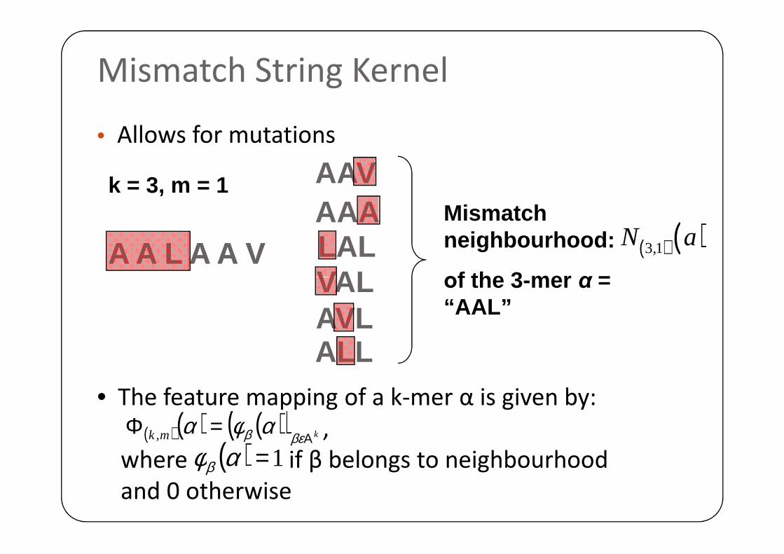
Mismatch String Kernel
• Allows for mutations
AAVAAALALVAL
Mismatch neighbourhood:
οf the 3 -mer α =
( ) ( )3,1N aA A L A A VA A L A A V
k = 3, m = 1
( )( ) ( )( ) kmk Α=Φ
βεβ αφα,
( ) 1=αφβ
• The feature mapping of a k-mer α is given by:
,
where if β belongs to neighbourhood
and 0 otherwise
VALAVLALL
οf the 3 -mer α = “AAL”

Mismatch String Kernel (cont.)
� The feature mapping of sequence x is given by:
� The (k,m)-mismatch kernel is given by:
( )( ) ( )( )∑−
=Φxamersk
mkmk xin
,, αφ
( )( ) ( )( ) ( )( )yxyxK mkmkmk ,,, ,, ΦΦ=

Mismatch Tree - An efficient data
Structure
� Representation of feature space as a tree
� Depth of tree: k
� Number of branches of each internal node:
lA =� Label of each branch: a symbol from A

Mismatch Tree- An efficient data
Structure (cont.)
Alphabet A = (A, V, L)
k = 3 A V L
A V L
Internal nodes: prefix of k-mer
A V L
A V L
AA AV AL
AAA AAV AAL
…
Leaf nodes: fixed k-mers

Mismatch Tree – Traversal (DFS)
0 0
A A
A L
L A
A
0 0
A L
Sequence: AALA
k = 3, m = 1
L
A L
L AA
0 1
L A
A
2
L
1
V
1
( ) ( ) )()(,, ycountxcountyxKyxK ⋅+←

Outline� Definitions & Background
� Proteins
� Remote Homology Detection
� SVMs
� Insides of the algorithm
� Feature mapping� Feature mapping
� Mismatch tree data structure
� Mismatch tree traversal
� Computational Efficiency
� Experiments
� Discussion

Efficiency – Space Complexity
� No need to store the entire tree
� For k = 7 1.28 billion nodes!
� No need to store all feature vectors � No need to store all feature vectors
� Kernel trick!

Efficiency – Time Complexity
• A fixed k-mer α has: k-mers to its neighbourhood
• , where
• M: number of sequences and
• n: the length of each sequence
• N: total length of the dataset
( )mmlkO
MnN =
• N: total length of the dataset
• Whole dataset: k-mers
• Worst case: perform updates to the kernel matrix
• Overall running complexity:
( )mmlNkO
( )2MO
( )mmlnkMO 2

System Pipeline
• Training Phase
– Compute the kernel matrix for all the training
sequences
– Normalize (divide by the length of the vectors)
– Train the SVM classifier– Train the SVM classifier
– Compute and store the k-mer scores of the
Support Vectors
• Testing Phase
– Compute the feature vector for each test datum
and predict its class in linear time
( ) ( )( ) ( )( )∑=
+ΦΦ=r
imkimkii bxxayxf
1,, ,

Experiments
� Benchmark dataset designed by Jaakkola et al. from
the SCOP database
� 33 Families
Superfamily
FamilyPos. Train Pos.
TestNegative Train
Experiments (cont.)
� Comparison to other methods:
� PSI-BLAST (mainly used for homology detection)
� SAM-T98
� Fisher-SVM (the state-of-the- art)

ROC Curve - ROC Scores
1
TP
1
TP0,7
0,8
ROC Score is the area
under the curve
0 FP 1 0 FP 1

Comparison of all methods

Family-by-family Comparison

Discussion
• Mismatch-SVM performs equally well with Fisher-
SVM method
• Mismatch-SVM much more efficient
• Efficiency: important issue
• Large real-world datasets• Large real-world datasets
• Multi-class prediction
• Accuracy increased by incorporating biological
knowledge

Questions ?Questions ?
Recommended


![Effective Face Recognition Using Bag of Features with ...bebis/JEI2016.pdf · SVM classifier is very high, we use a linear SVM solver, Pegasos [27], with the help of additive kernels,](https://img.pdfslide.us/doc/110x75/5e78c72a2c30a75d19512d7c/effective-face-recognition-using-bag-of-features-with-bebis-svm-classifier.jpg)