Miniaturization, Integration, Flight Testing, and
Performance Analysis of a Scalable Autonomous GPS-
Guided Parafoil System for Targeted Payload Return
A Project
Presented to
The Faculty of the Department of Mechanical and Aerospace Engineering
San José State University
In Partial Fulfillment
of the Requirements for the Degree
Master of Science in Aerospace Engineering
by
Joshua E. Benton
May 2012

© 2012
Joshua E. Benton
ALL RIGHTS RESERVED
Miniaturization, Integration, Flight Testing, and
Performance Analysis of a Scalable Autonomous GPS-
Guided Parafoil System for Targeted Payload Return
Joshua E. Benton1
San Jose State University, San Jose, CA, 95192
An autonomous parafoil system design is presented as a solution to the final descent
phase of an on-demand International Space Station (ISS) sample return concept. The system
design is tailored to meet specific constraints defined by a larger study at NASA Ames
Research Center, called SPQR (Small Payload Quick-Return). Building on previous work in
small, autonomous parafoil systems development, an SPQR-compatible evolution of an
existing advanced parafoil delivery system is designed, built, and test-flown to evaluate
performance of the new control system hardware and software. Results of the control system
tests are presented, and applicability of the test article to actual spaceflight conditions is
discussed.
1 Graduate Student, San Jose State University, One Washington Square, San Jose, CA.
136
Acknowledgments
I have been particularly fortunate in my life thus far with the opportunities and remarkable people I have
encountered along the way. Without the love, support, encouragement, and generous, selfless mentoring from these
individuals, I could not have achieved even a fraction of my humble accomplishments, and I am forever indebted to
their kindness.
First and foremost, I would like to thank my family for their unending love and support. They have always been
the foundation that holds me up through all of my successes, failures, challenges, and triumphs in life. Their
importance to me cannot possibly be summed up in a couple of short sentences, so I will spare the reader from any
attempt to do so.
Second, I would like to thank Marc Murbach, without whom I surely would not be writing this work. In the five
years I have known Marc, his mentoring has provided too many new opportunities and remarkable experiences to
count. Marc was solely responsible for bringing me to NASA’s Ames Research Center as an intern several years
ago, and thanks to his unbreakable enthusiasm and trust in our team’s abilities to achieve extraordinary goals, I got
to be involved in real “rocket science.” Marc is truly one-of-a-kind, and I am deeply grateful for his guidance and
friendship.
I would also like to thank Dr. Mourtos and Dr. Papadopoulos for sharing their immense knowledge, with an
obvious and genuine desire to help their students learn and succeed—not just scholastically, but also in their future
lives and careers.
The work in this project would not have been possible without the contributions from Dr. Oleg Yakimenko and
Chas Hewgley, for not only helping us learn the basics of their Snowflake system, but also allowing me to build
upon their research for this project. Dr. Yakimenko has been instrumental in assisting my work, from coordinating
the opportunities to drop our payloads from the Arcturus UAVs, to helping me retrieve payloads from drop tests that
didn’t go quite as planned. His presence at the most recent Idaho balloon test was also greatly appreciated.
Dr. David Atkinson, Kevin Ramus, and the entire University of Idaho VAST team deserve special thanks and
recognition, for providing the launch opportunities to test the parafoil system from very high altitudes beneath their
balloons. The level of support and knowledge required to orchestrate, execute, and recover payloads from the
balloon launches is immense, and their launch expertise and gracious support in flying our payloads is an asset of
extraordinary value.
Finally, I’d like to thank the crew of Arcturus UAV, for allowing me the use of their highly-advanced UAV
systems to carry and drop my payloads from altitudes beyond anything I could hope to achieve with my own R/C
helicopter. Being able to use their cutting-edge technology for testing the flight performance of my control system is
a privilege that I do not take for granted, and appreciate immensely.
2
Table of Contents Nomenclature ................................................................................................................................................................ 4
Acronyms ...................................................................................................................................................................... 5
I. Introduction ........................................................................................................................................................... 6
II. Background ...................................................................................................................................................... 7
A. Motivation ........................................................................................................................................................ 7
B. Objectives ......................................................................................................................................................... 9
III. Literature Review and Current State of Development .................................................................................... 10
A. A Brief History of Parachutes ........................................................................................................................ 10
B. Parachutes and Space Payload Recovery........................................................................................................ 11
C. Autonomous Parafoil Systems for Payload Delivery ..................................................................................... 11
D. Parafoil Systems for Small Payloads with Improved Precision ...................................................................... 12
E. Past and Current Work with SPQR and the Snowflake Parafoil System ........................................................ 13
F. Summarized Results of Previous System V.1 Flight Tests with Simple Control Algorithm .......................... 15
1. Balloon Flight Test #1 – Oct. 16, 2010 ...................................................................................................... 17
2. Balloon Flight Test #2 – April 23, 2011 .................................................................................................... 19
3. Balloon Flight Test #3 – Aug. 19, 2011 ..................................................................................................... 21
4. Balloon Flight Test #4 – September 13, 2011 ............................................................................................ 22
IV. System V.2 Mechanical Steering Design ....................................................................................................... 25
A. Design Context ............................................................................................................................................... 25
B. System V.2 Design Constraints and Necessary Improvements to Existing System V.1 Architecture ........... 26
1. Volumetric Envelope for PCTCU Compatibility ....................................................................................... 26
2. Mass ........................................................................................................................................................... 28
3. Parafoil and GPS Antenna Deployment Considerations ............................................................................ 28
4. Thermal and Vacuum Considerations ........................................................................................................ 29
5. Special Considerations for ISS Compatibility ............................................................................................ 30
C. The New System V.2 Design ......................................................................................................................... 30
1. Design Overview ........................................................................................................................................ 30
2. Design Improvements: Size, Mass, and Elimination of Line Tensioning System..................................... 33
3. Servo Selection .......................................................................................................................................... 36
4. Structural Design ........................................................................................................................................ 39
V. System V.2 Electronics System Design .......................................................................................................... 41
A. Design Context ............................................................................................................................................... 41
B. Design Details and Block Diagram ................................................................................................................ 42
C. Additional Electrical Design Considerations for Space-Flight Use ................................................................ 45
VI. Flight Software Development ......................................................................................................................... 48
A. Overview ........................................................................................................................................................ 48
B. Software Control Algorithm Flow Charts ...................................................................................................... 49
C. Detailed Description of Control Methodology ............................................................................................... 59
3
1. Control Software Inputs ............................................................................................................................. 59
2. Main Control Loop – “simple_control()” ................................................................................................... 62
3. Nominal Flight Guidance Routine – “steerToTarget()” ............................................................................. 64
4. Landing Routine – “landingRoutine()” ...................................................................................................... 74
5. Landing Flare Routine – “landingFlare()” ................................................................................................. 77
D. Flight Test Results .......................................................................................................................................... 78
1. Testing Methods ......................................................................................................................................... 78
2. Flight Test Data and Steering System Performance ................................................................................... 86
VII. Discussion and Future Work ........................................................................................................................ 113
VIII. Conclusion .................................................................................................................................................... 114
IX. References .................................................................................................................................................... 115
Appendix A: Complete Flight Software .................................................................................................................... 116
Appendix B: Addendum - High Altitude Balloon Flight Results, May 19, 2012....................................................... 132
4
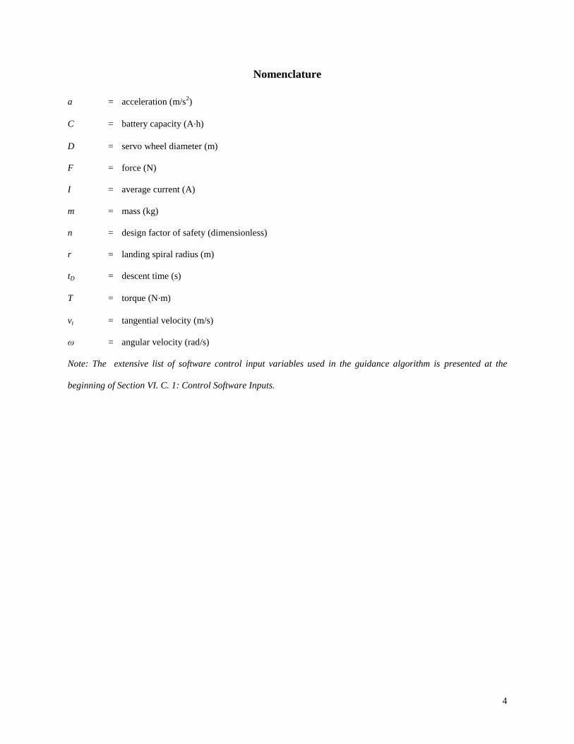
Nomenclature
a = acceleration (m/s2)
C = battery capacity (A·h)
D = servo wheel diameter (m)
F = force (N)
I = average current (A)
m = mass (kg)
n = design factor of safety (dimensionless)
r = landing spiral radius (m)
tD = descent time (s)
T = torque (N·m)
vt = tangential velocity (m/s)
ω = angular velocity (rad/s)
Note: The extensive list of software control input variables used in the guidance algorithm is presented at the
beginning of Section VI. C. 1: Control Software Inputs.

5
Acronyms
APRS = Automatic Packet Reporting System
AGL = Above Ground Level
COTS = Commercial Off-The-Shelf
GN&C = Guidance, Navigation, and Control
GPS = Global Positioning System
IMU = Inertial Measurement Unit
ISS = International Space Station
microSD = micro Secure Digital
PCTCU = Payload Containment and Thermal Control Unit
PWM = Pulse-Width Modulation
R/C = Radio-Controlled
SPQR = Small Payload Quick-Return
TOW = Time of Week
UAV = Unmanned Aerial Vehicle
UTC = Coordinated Universal Time
VAST = Vandal Atmospheric Science Team
6
I. Introduction
parafoil is a special type of airfoil that is typically made of cloth and relies on dynamic pressure in flight to
retain its shape. Due to their being non-rigid (and therefore foldable and packable), parafoils lend
themselves very well to applications where controlled descent is required, but limited stowage is available for any
sort of traditional wing structure. Also, compared to a traditional round parachute, parafoils have much greater
directional control, improved glide performance, and the ability to adjust rate of descent by deforming the shape of
the airfoil via control (or “toggle”) lines. These attributes of parafoils have made them very popular for human aerial
descent, where the entire parafoil as well as a redundant backup can be stowed in a backpack and deployed rapidly
when necessary. In addition to manned applications, unguided parafoils provide an attractive means to deliver a
variety of payloads (e.g. military supplies, emergency equipment, food packages) to remote or inaccessible locations
with a moderate degree of accuracy. This accuracy can be further improved by including an autonomous control
system on the payload, which can effectively steer the parafoil in the same fashion as a human would, guiding it
with a higher degree of precision to its landing point. In the last decade, several independent research efforts have
focused on doing exactly this, providing complete, intelligent parafoil systems which autonomously steer themselves
to a pre-defined landing point to deliver payloads—typically, military supplies. Recent research efforts have
improved accuracy of these systems from a few kilometers landing error to orders of magnitude less, depending on
prevailing winds and initial drop altitude.
A
7
II. Background
A. Motivation
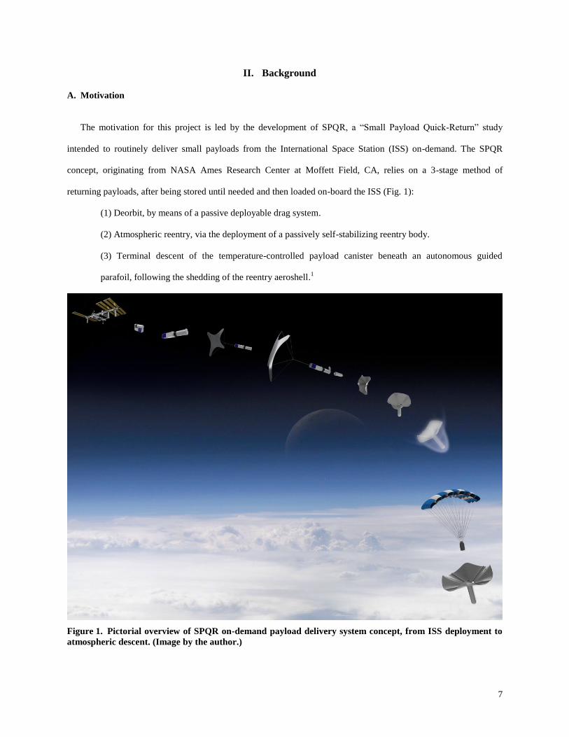
The motivation for this project is led by the development of SPQR, a “Small Payload Quick-Return” study
intended to routinely deliver small payloads from the International Space Station (ISS) on-demand. The SPQR
concept, originating from NASA Ames Research Center at Moffett Field, CA, relies on a 3-stage method of
returning payloads, after being stored until needed and then loaded on-board the ISS (Fig. 1):
(1) Deorbit, by means of a passive deployable drag system.
(2) Atmospheric reentry, via the deployment of a passively self-stabilizing reentry body.
(3) Terminal descent of the temperature-controlled payload canister beneath an autonomous guided
parafoil, following the shedding of the reentry aeroshell.1
Figure 1. Pictorial overview of SPQR on-demand payload delivery system concept, from ISS deployment to
atmospheric descent. (Image by the author.)
8
The first two return phases exist at varying levels of maturity. The passive drag deorbit system has yet to be
tested in a space-like environment, but the self-stabilizing reentry vehicle has undergone multiple successful flight
tests as a series of sounding rocket payloads.2 The third and final phase, terminal guided descent, is where the focus
of this project lay. To mature this final phase of the SPQR concept, an autonomous parafoil system which satisfies
the demands of the volumetric, environmental (space-flight), and landing precision requirements must be developed.
A handful of autonomous parafoil systems exist and their guidance routines are highly refined (though also
proprietary), but none of these available systems completely satisfy the specific set of unique challenges and
requirements imposed by the SPQR design scenario.
In addition, a scalable version of the proposed parafoil system would have many other aerospace applications
beyond the SPQR system, including, for example, greatly simplified retrieval of sounding rocket payloads. At
present, such payloads launched from NASA’s Wallops Flight Facility typically rely on recovery from the ocean by
small fishing vessels (if they are to be recovered at all), which is time-consuming, inefficient, and occasionally
unsuccessful. Sounding rockets provide a relatively inexpensive means to test small payloads in a space
environment, but the additional cost of telemetry and communications, and the difficulty of recovering payloads,
make them far less attractive for deployable experiments. A reliable precision return system for deployable payloads
could make on-board data logging a feasible alternative to expensive ground-based communications, and
significantly reduce the associated costs of sounding rocket experimentation. Also, on-board logging can record an
enormous quantity of data at very high bitrates, enabling greater experiment precision if the data has a high
probability of being recovered.
A further application of a miniature, lightweight, autonomous parafoil system is the increasingly-common use of
high-altitude weather balloons for amateur experimenters. Balloon payloads routinely carry parachutes for safe
recovery after the bursting of the balloon, but the final landing spot of the payload is at the mercy of the winds it
encounters on descent. Typically, the recovery of the payload is the most challenging aspect of balloon
experimentation, and losing a payload in an unexpected landing location is not at all a rare occurrence. If the
standard payload return parachute was replaced with a very small, autonomous guided parafoil system, payloads
could be returned to a pre-defined location and eliminate the elaborate routine of chase vehicles and search crews
that accompany most balloon launches.
9
B. Objectives
The objectives of this multi-faceted project are as follows:
1) Re-design and miniaturize an existing autonomous parafoil control system and its associated control
line rigging to fit within the volumetric constraints of the SPQR payload canister.
2) Develop new autonomous control software to steer and land the parafoil at a target GPS coordinate on
the ground from any starting point, requiring only the target coordinates and target elevation as inputs.
3) Verify the performance of the new control system hardware and software via flight testing from an
altitude sufficient to determine control characteristics, and demonstrate the ability of the system to manage
flight disturbances such as crosswinds.
4) Discuss strategies to enable the use of the parafoil system in a challenging space-purposed scenario,
including design considerations to ensure compatibility with ISS safety protocol.
10
III. Literature Review and Current State of Development
A. A Brief History of Parachutes
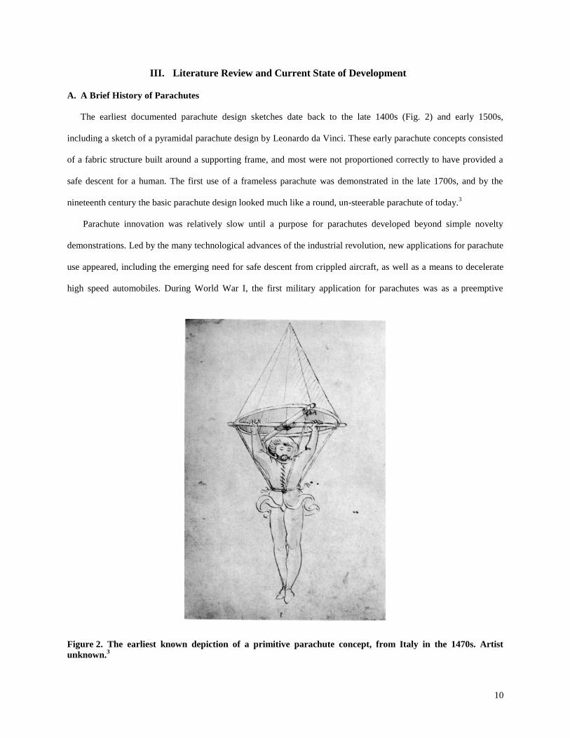
The earliest documented parachute design sketches date back to the late 1400s (Fig. 2) and early 1500s,
including a sketch of a pyramidal parachute design by Leonardo da Vinci. These early parachute concepts consisted
of a fabric structure built around a supporting frame, and most were not proportioned correctly to have provided a
safe descent for a human. The first use of a frameless parachute was demonstrated in the late 1700s, and by the
nineteenth century the basic parachute design looked much like a round, un-steerable parachute of today.3
Parachute innovation was relatively slow until a purpose for parachutes developed beyond simple novelty
demonstrations. Led by the many technological advances of the industrial revolution, new applications for parachute
use appeared, including the emerging need for safe descent from crippled aircraft, as well as a means to decelerate
high speed automobiles. During World War I, the first military application for parachutes was as a preemptive
Figure 2. The earliest known depiction of a primitive parachute concept, from Italy in the 1470s. Artist
unknown.3
11
rescue device for observation balloon crewmen, who were frequent targets of enemy fighter aircraft. Due to the
danger of the flammable hydrogen used to provide buoyancy for these balloons, observation officers would depart
the balloons via parachute at the first sighting of enemy aircraft, and the tethered balloon would then be reeled-in by
ground crew and deflated as quickly as possible. The first use of parachutes to drop troops behind enemy lines was
conducted by Italy in 1927, and by World War II, air drops of troops by parachute had become much more
common.3
B. Parachutes and Space Payload Recovery
The first successful recovery of an object from orbit occurred under the U.S.’s top-secret CORONA spy satellite
program. This program operated from 1959 to 1972, existing primarily as a means to keep a watchful eye on the
nuclear weapons progress of the Soviet Union. The satellites used by CORONA carried highly-advanced film
camera systems which snapped surveillance photographs from orbit, and the film was then returned by a reentry
capsule and parachute system. A small decelerator parachute deployed as high as 65,000 ft. altitude, and a main
chute was deployed 10,000 feet lower. Finally, the entire film “bucket” and parachute were snatched from the air by
a large, specially-equipped Air Force airplane.4
With the growth of the US space program during the same era, the use of parachutes to safely return space
payloads on their final stages of descent became commonplace. The manned Mercury, Gemini, and Apollo capsules
used parachute recovery systems as well. Currently, modern space missions (manned, such as the Russian Soyuz
capsule, or unmanned) frequently make use of parachutes for slowing their payload’s final atmospheric descent.
C. Autonomous Parafoil Systems for Payload Delivery
Currently, a great deal of research has gone into autonomous payload delivery systems utilizing steerable
parachutes. The parachutes typically used for these systems are rectangular, structured chutes consisting of a series
of open cells which, when inflated, form the parachute into a wing-like structure with a distinct airfoil cross-section.
These particular parachutes are known as parafoils, and they offer significant advantages for precise targeting of
descending payloads. Compared to a traditional round parachute, parafoils operate more like an aircraft wing,
enabling greater precision in steering maneuvers that are executed by warping the trailing edge of the parafoil much
like the aileron of an airplane. Also, parafoils fly with a significant component of forward velocity, and this glide
12
slope allows a parafoil to cover a range of horizontal distance over the ground during its descent. The steerability,
glide capability, and the light weight and packable stowage attributes of a parafoil make it a very attractive option
for payload delivery where size, weight, and mechanical complexity need to be kept to a minimum.
Both commercial and military versions of payload delivery parafoil systems exist and are in routine use. The
parafoil systems enable precise air-drop of supplies, emergency medical equipment, and other important payloads in
areas where landing precision must be maximized, either due to terrain or enemy presence. Compared to older,
round-canopy air-drop pallets, guided parafoil systems enable air-drops to occur at a much higher (and thus safer
altitude) while providing a higher degree of landing precision. Collectively, the U.S. military versions of these
systems are called JPADS (Joint Precision Airdrop System)5, and a typical example is MMIST’s Sherpa.
10 Of the
commercial parafoil system options, most exist for payloads on the order of hundreds to thousands of pounds. The
lightest-weight military JPADS system is specified for payloads of 10-100 pounds.5
D. Parafoil Systems for Small Payloads with Improved Precision
With modern GPS systems, miniaturized integrated avionics systems and IMUs, and advanced guidance
algorithms that can easily be run by inexpensive, readily-available integrated microprocessor boards, it has become
feasible to design a highly-miniaturized parafoil payload delivery system with excellent targeting accuracy. While
most existing commercial systems are tailored to payloads of 10 to 100 lbs. or greater, there exists a need for
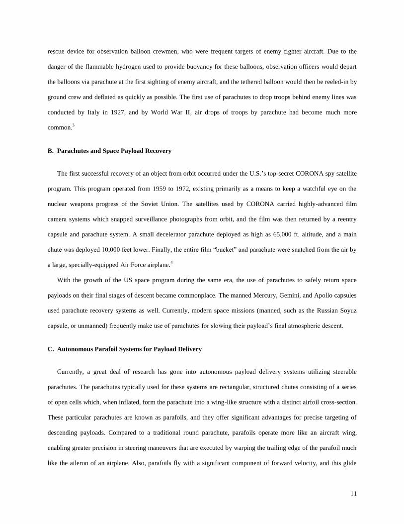
smaller, lighter, and more volume- and mass-efficient systems as well. One such system, developed jointly by
researchers at the University of Huntsville in Alabama and the Naval Postgraduate School in California, is currently
being tested with payloads on the order of 0 to 10 lbs. This system, dubbed Snowflake (Fig. 3), utilizes a parafoil
approximately 6 feet in span when inflated, and relies on GN&C electronics roughly the size of a deck of cards.6,7
13
The Snowflake is particularly advanced in its targeting algorithm, enabling unprecedented landing accuracies
within a 10 m circle from an initial drop altitude of 1,900 ft. AGL at a velocity of approximately 80 mph.8 These
extreme levels of precision are accomplished by real-time generation of flight trajectories by the Snowflake’s
GN&C system, which updates flight parameters based on wind estimations and atmospheric conditions in its
descent, as well as optimizing the final up-wind turn as it is being executed to ensure both a soft and precise
landing.7
E. Past and Current Work with SPQR and the Snowflake Parafoil System
Prior to the authoring of this paper, the team members developing the NASA Small Payload Quick Return
(SPQR) concept (including the author) have been graciously assisted by Snowflake researchers Dr. Oleg Yakimenko
and Chas Hewgley of the Naval Postgraduate School in Monterey, California, in testing a derivative of Snowflake,
suitable for SPQR’s terminal descent phase. In its first design iteration, a basic facsimile of the Snowflake’s
Figure 3. The advanced, high-precision, miniature Snowflake Aerial Drop System.8
14
mechanical systems was fabricated, and a new control board was implemented for the GN&C systems. Due to the
challenge of porting the existing highly-advanced guidance routines from one board to another (with differing
coding languages), the original SPQR variant of Snowflake was first programmed with an extremely simple steering
algorithm to serve as a basic prototype. This basic algorithm reads the GPS heading from the control board,
compares it to a predefined heading that it is programmed to follow, and then commands a non-proportional right
turn, left turn, or straight flight based on this data. For clarity throughout the rest of this work, this older version of
the Snowflake-derived device will be referred to as “System V.1,” and the improved design, which is the focus of
this paper, will be referred to as “System V.2.”
The basic simple-control system, System V.1, has been tested in multiple air-drops from a UAV at altitudes up to
3,000 ft. AGL, and development has also been on-going with the University of Idaho in high-altitude balloon drop-
tests of the device from a peak of 42,000 ft. To date, System V.1 has been flown from University of Idaho’s VAST
balloons on four separate occasions, beginning in October 2010. Tests from the UAV drops were generally
successful with rapid parafoil deployment and inflation, and the device maintained the correct heading throughout
its descent. However, the extreme simplicity of the steering algorithm made it incapable of correcting for moderate
crosswinds, causing a steady drift away from the desired heading in their presence. The balloon drops have proven
to be more challenging, due to a variety of factors: shroud lines have tangled during ascent, snags have occurred on
the cut-down system, and, in some cases, parafoil inflation was delayed or failed altogether despite ideal drop
conditions.
To develop a valid proof-of-concept system for the SPQR study, more development is necessary. Though the
original Snowflake system is already compact, a significant reduction in size is necessary to fit within the volumetric
constraints of the SPQR sample return canister. This can be achieved by a more efficient line-rigging and tensioning
scheme, by using smaller servos, and by placing the GN&C control board closer to the mechanical systems, as
shown in Section IV: System V.2 Mechanical Steering System Design.
Finally, the many challenging aspects of designing a system for spaceflight scenarios must be considered.
Though the parafoil itself will only operate in an atmospheric environment, it will be subjected to the full gamut of
space transport to and from the ISS within the complete SPQR system. These considerations include material
restrictions based on vacuum outgassing, battery restrictions imposed by launch vehicles as well as the ISS, stored
energy constraints, direct solar heating during deorbit, and appropriate heat shielding to survive reentry. In the work
15
that follows, these concerns will be discussed in the design description of the System V.2 SPQR parafoil descent
system.
The end product of this project is a complete, functional prototype of an autonomous parafoil return system,
compatible in size, shape, mass, and method of operation with the SPQR sample return canister. This “SPQR-ready”
prototype was originally to be tested by release from a high-altitude balloon, but unfortunately, unfavorable weather
and wind conditions delayed the launch for over a month, preventing high-altitude flight testing prior to completion
of this paper. (Addendum: this balloon test was conducted on May 19, 2012, and a brief description of the results is
presented in Appendix B.) However, nearly 40 drop tests from an R/C helicopter as well as several drops from a
UAV at altitudes up to 2,000 ft. AGL were used to refine and verify the performance of the steering software.
Results of these tests are presented in Section VI, Part D: Flight Test Results.
Throughout the following presentation of the design work, a distinction is made wherever necessary between the
flight-test article as just described, and the additional considerations required to create a full-fledged space qualified
system.
F. Summarized Results of Previous System V.1 Flight Tests with Simple Control Algorithm
To date, the System V.1 architecture has been released several times from a UAV, from altitudes ranging from
1,500 to 3,000 ft. AGL. These UAV drops were the first functional validation tests of the “simple control” steering
algorithm, and confirmed that the Snowflake-derived device (utilizing a different control board and servos) was
working as expected in terms of basic functionality. The first several drops indicated that the steering control gains
were too large for the non-proportional control scheme, causing the device to overcorrect with every turn. This
resulted in the parafoil system continuously yawing left and right in an over-controlled oscillation from release to
landing. The steering input gains were gradually reduced in the software code until System V.1 showed no more
tendency to over-steer.
Having demonstrated basic system performance and the ability to fly toward a pre-specified heading with the
UAV drops, the next goal was to determine the flight characteristics of the parafoil over a much greater altitude
range—approximately 50,000 ft. to ground level. Because the SPQR parafoil system is intended to provide final
trajectory correction for a payload returned from orbit, the maximum trajectory correction possible will be achieved
by deploying the parafoil at as high an altitude as possible. It is to be expected that parafoils, by their self-inflating
16
nature, do not perform well with low dynamic pressure. Because atmospheric density decreases as a function of
altitude, there is a threshold beyond which the SPQR system parafoil will not be operable. Also, as was found in the
next series of flight tests, a challenge even greater than flying a small parafoil in low atmospheric density regimes is
actually getting the parafoil to inflate at all. If the parafoil fails to inflate upon initial release at high altitude, this
testing has demonstrated that tumbling and tangling occur almost immediately, thus preventing the parachute from
inflating even after it descends into the lower, denser atmosphere.
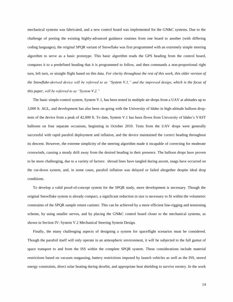
The high-altitude testing mentioned in the previous paragraph was carried out in Idaho and Washington (Fig. 4),
with the help of the University of Idaho’s VAST balloon team. Prior to the authoring of this paper, four balloon
flights had been conducted with the System V.1 device, with varying levels of success. All of these balloon flights
used the simple non-proportional, fixed-heading steering algorithm previously described, and all were attempts to
quantify the parafoil performance over a broad altitude range by analyzing the detailed data stored on the onboard
data log. The ease or difficulty of inflating the parafoil at these altitudes was also to be investigated. For every flight,
high-definition video was captured with up-looking and 45-degree down-looking HD video cameras, data was
Figure 4. Above the clouds: a view over eastern Washington, near the Idaho border, from the balloon’s
perspective.
17
logged by the Ryan Mechatronics Monkey control board (with the exception of the first balloon flight), and the
parafoil system was tracked via the APRS amateur radio network to facilitate recovery. The following are brief
summaries of each flight; the results, failures and successes observed; and the steps taken to improve the system for
the next flight:
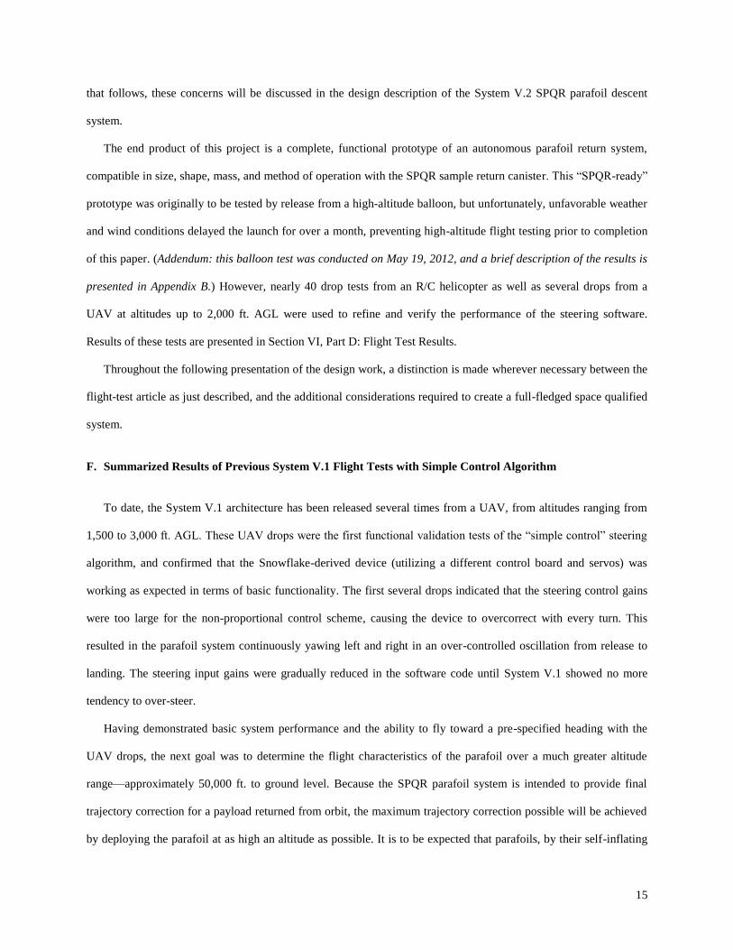
1. Balloon Flight Test #1 – Oct. 16, 2010
This was the first high-altitude balloon test of System V.1. The parafoil system failed to separate
from the balloon, even though it can be seen and heard on the on-board video that the separation charge fired
as expected at altitude. Also, no visible tangles were present in the shroud lines, so the exact reason for the
parafoil system not separating is still unknown. Because separation from the balloon never occurred, the
entire payload was lifted to burst altitude with the balloon (approximately 80,000 ft.). The instant of balloon
burst is shown in Fig. 5.
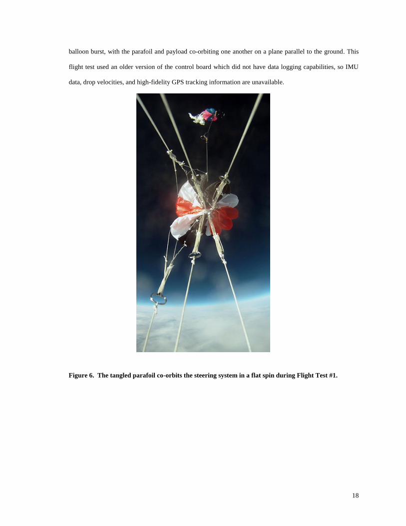
Upon burst, the combined package of parafoil system, balloon tracking system, and attachment lines began a
rapid flat-spin, and the tangled system fell to the ground in this state. Fig. 6 shows the system following
Figure 5. Balloon at the instant of burst viewed from on-board video camera during Balloon Flight Test #1
after failed release.
18
balloon burst, with the parafoil and payload co-orbiting one another on a plane parallel to the ground. This
flight test used an older version of the control board which did not have data logging capabilities, so IMU
data, drop velocities, and high-fidelity GPS tracking information are unavailable.
Figure 6. The tangled parafoil co-orbits the steering system in a flat spin during Flight Test #1.
19
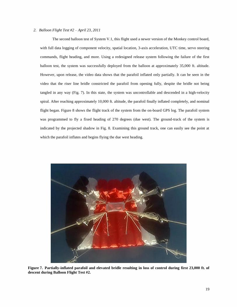
2. Balloon Flight Test #2 – April 23, 2011
The second balloon test of System V.1, this flight used a newer version of the Monkey control board,
with full data logging of component velocity, spatial location, 3-axis acceleration, UTC time, servo steering
commands, flight heading, and more. Using a redesigned release system following the failure of the first
balloon test, the system was successfully deployed from the balloon at approximately 35,000 ft. altitude.
However, upon release, the video data shows that the parafoil inflated only partially. It can be seen in the
video that the riser line bridle constricted the parafoil from opening fully, despite the bridle not being
tangled in any way (Fig. 7). In this state, the system was uncontrollable and descended in a high-velocity
spiral. After reaching approximately 10,000 ft. altitude, the parafoil finally inflated completely, and nominal
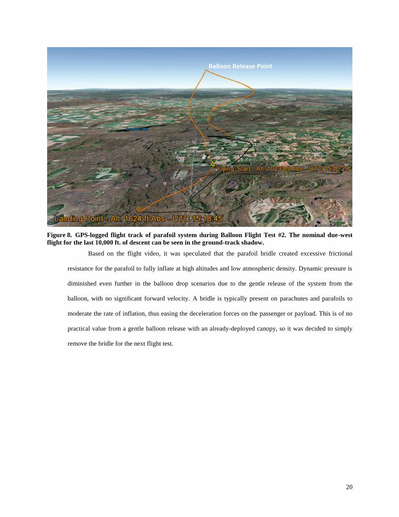
flight began. Figure 8 shows the flight track of the system from the on-board GPS log. The parafoil system
was programmed to fly a fixed heading of 270 degrees (due west). The ground-track of the system is
indicated by the projected shadow in Fig. 8. Examining this ground track, one can easily see the point at
which the parafoil inflates and begins flying the due west heading.
Figure 7. Partially-inflated parafoil and elevated bridle resulting in loss of control during first 23,000 ft. of
descent during Balloon Flight Test #2.
20
Based on the flight video, it was speculated that the parafoil bridle created excessive frictional
resistance for the parafoil to fully inflate at high altitudes and low atmospheric density. Dynamic pressure is
diminished even further in the balloon drop scenarios due to the gentle release of the system from the
balloon, with no significant forward velocity. A bridle is typically present on parachutes and parafoils to
moderate the rate of inflation, thus easing the deceleration forces on the passenger or payload. This is of no
practical value from a gentle balloon release with an already-deployed canopy, so it was decided to simply
remove the bridle for the next flight test.
Figure 8. GPS-logged flight track of parafoil system during Balloon Flight Test #2. The nominal due-west
flight for the last 10,000 ft. of descent can be seen in the ground-track shadow.
21
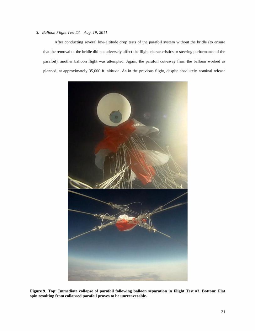
3. Balloon Flight Test #3 – Aug. 19, 2011
After conducting several low-altitude drop tests of the parafoil system without the bridle (to ensure
that the removal of the bridle did not adversely affect the flight characteristics or steering performance of the
parafoil), another balloon flight was attempted. Again, the parafoil cut-away from the balloon worked as
planned, at approximately 35,000 ft. altitude. As in the previous flight, despite absolutely nominal release
Figure 9. Top: Immediate collapse of parafoil following balloon separation in Flight Test #3. Bottom: Flat
spin resulting from collapsed parafoil proves to be unrecoverable.
22
conditions, the parafoil failed to inflate. The video data shows the parafoil falling gently away from the
balloon and immediately collapsing upon itself (much like it would in vacuum), and the whole system
quickly enters a high-yaw-rate flat spin. Fig. 9, top, shows System V.1 a moment after release, with the
balloon drifting away, and the parafoil already collapsed into a loosely crumpled mass. Unlike the previous
flight, where the parafoil eventually inflated and recovered, the crumpled parachute system continued in a
rapid flat-spin all the way to the ground. Fig. 9, bottom, shows the view of the collapsed parafoil canopy
from the on-board camera during this energetic flat-spin.
4. Balloon Flight Test #4 – September 13, 2011
All balloon flights prior to this test encountered partial or total failures due to delayed or failed
parafoil inflation. Based on the video data, it appeared that the lack of inflation was caused by several
factors: low atmospheric density at altitude, resulting in diminished dynamic pressure and less total drag to
inflate the parafoil cells and keep the parafoil above the payload; lack of forward velocity upon release from
the balloon, also causing diminished dynamic pressure to inflate the parafoil cells; and the initial collapsed
state of the parafoil upon release, which inhibits air flow into the parafoil cells and makes inflation
exceedingly difficulty in the high altitude, low density release regime.
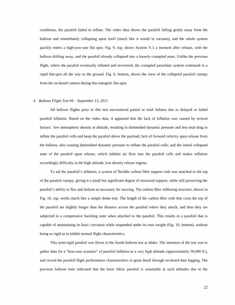
To aid the parafoil’s inflation, a system of flexible carbon fiber support rods was attached to the top
of the parafoil canopy, giving it a small but significant degree of structural support, while still preserving the
parafoil’s ability to flex and deform as necessary for steering. The carbon fiber stiffening structure, shown in
Fig. 10, top, works much like a simple dome tent. The length of the carbon fiber rods that cross the top of
the parafoil are slightly longer than the distance across the parafoil where they attach, and thus they are
subjected to a compressive buckling state when attached to the parafoil. This results in a parafoil that is
capable of maintaining its basic curvature while suspended under its own weight (Fig. 10, bottom), without
being so rigid as to inhibit normal flight characteristics.
This semi-rigid parafoil was flown in the fourth balloon test at Idaho. The intention of the test was to
gather data for a “best-case scenario” of parafoil inflation at a very high altitude (approximately 50,000 ft.),
and record the parafoil flight performance characteristics in great detail through on-board data logging. The
previous balloon tests indicated that the basic fabric parafoil is unsuitable at such altitudes due to the
23
difficulty of inflating the parafoil cells, but greatly improved inflation reliability and therefore increased
down-range trajectory correction could be gained by assisting the parafoil’s inflation with the rigidizing
structure. By supporting the shape of the parafoil with the structure, the tendency for the parafoil to collapse
is eliminated, and the structure also helps to keep the parafoil cell entrances open, aiding inflation.
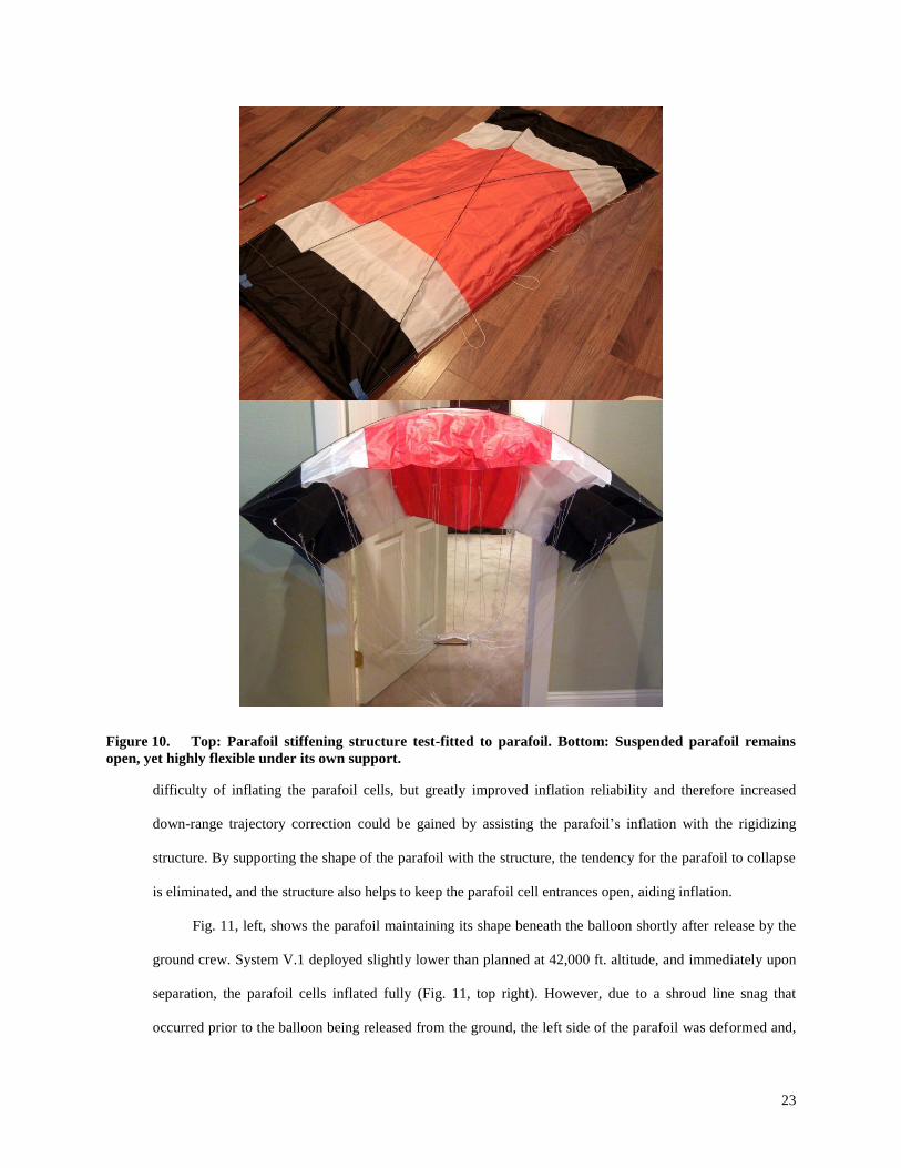
Fig. 11, left, shows the parafoil maintaining its shape beneath the balloon shortly after release by the
ground crew. System V.1 deployed slightly lower than planned at 42,000 ft. altitude, and immediately upon
separation, the parafoil cells inflated fully (Fig. 11, top right). However, due to a shroud line snag that
occurred prior to the balloon being released from the ground, the left side of the parafoil was deformed and,
Figure 10. Top: Parafoil stiffening structure test-fitted to parafoil. Bottom: Suspended parafoil remains
open, yet highly flexible under its own support.
24
again, a spiraling flat-spin ensued. Unfortunately, the system continued this spiral until only a few thousand
feet above ground level, at which point a sharp “snap” can be heard and seen in the video. The snagged line
is then suddenly released, the uncontrollable spiraling immediately ceases, and the system flies nominally
for a short time until landing (Fig. 11, bottom right). Consequently, the data obtained from this flight was no
more useful than the data obtained from the earlier UAV drops due to the very low altitude of nominal
operation.
Figure 11. Left: Rigidized parafoil maintains its shape beneath balloon payload train. Top Right: Rigidized
parafoil structure immediately inflates upon separation from balloon at 42,000 ft. altitude, but a line snag
causes an uncontrollable spiral. Bottom Right: Rigidized parafoil in nominal flight after snag is freed at
approx. 3000 ft. altitude.
25
IV. System V.2 Mechanical Steering Design
A. Design Context
Applied to the SPQR concept, there are a number of factors influencing the mechanical design of the complete
parafoil return system which must be considered. These include physical shape and size, minimization of mass to the
greatest extent possible, deployment considerations for the parafoil and GPS antenna, the operational environment
of the device from launch to return (e.g. thermal and vacuum), and additional specific constraints that would be
imposed by safety standards for transportation to (and stowage within) the ISS.
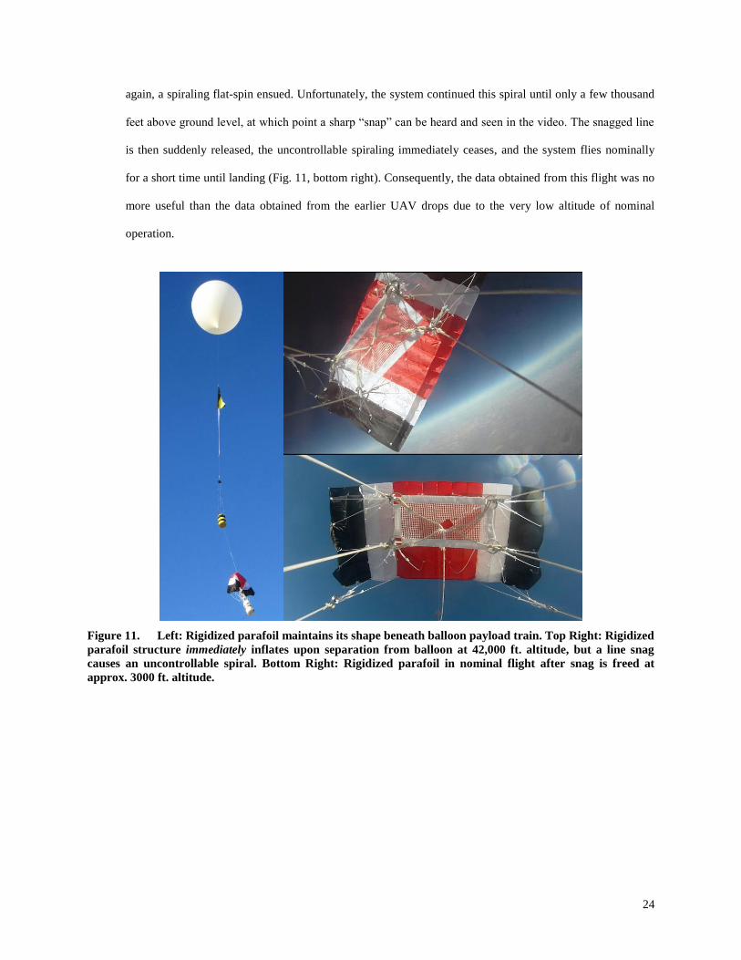
Though very compact compared to most existing autonomous parafoil return systems, the current Snowflake
control system architecture and the prototype System V.1 are both physically larger than the entire volume available
for the control system and stowed parafoil inside SPQR. This is mainly attributable to the fact that both are
development units, and durability, ease-of-assembly, and internal access for test modifications were of greater
concern than packaging optimization. Because of this, there is significant potential for volumetric reduction.
Figure 12. Existing System V.1 balloon test system (left) compared to available volume for both the SPQR-
specific System V.2 and its parafoil stowage.
26
B. System V.2 Design Constraints and Necessary Improvements to Existing System V.1 Architecture
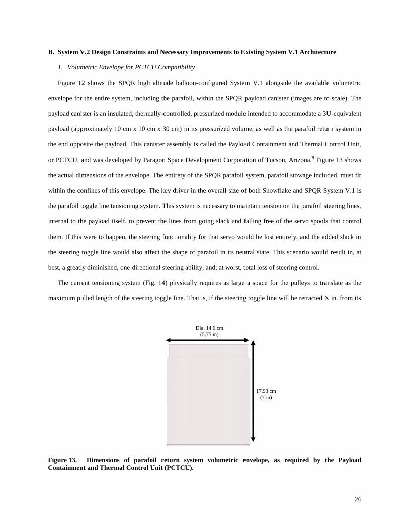
1. Volumetric Envelope for PCTCU Compatibility
Figure 12 shows the SPQR high altitude balloon-configured System V.1 alongside the available volumetric
envelope for the entire system, including the parafoil, within the SPQR payload canister (images are to scale). The
payload canister is an insulated, thermally-controlled, pressurized module intended to accommodate a 3U-equivalent
payload (approximately 10 cm x 10 cm x 30 cm) in its pressurized volume, as well as the parafoil return system in
the end opposite the payload. This canister assembly is called the Payload Containment and Thermal Control Unit,
or PCTCU, and was developed by Paragon Space Development Corporation of Tucson, Arizona.9 Figure 13 shows
the actual dimensions of the envelope. The entirety of the SPQR parafoil system, parafoil stowage included, must fit
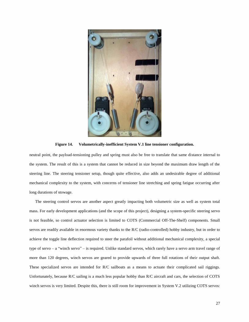
within the confines of this envelope. The key driver in the overall size of both Snowflake and SPQR System V.1 is
the parafoil toggle line tensioning system. This system is necessary to maintain tension on the parafoil steering lines,
internal to the payload itself, to prevent the lines from going slack and falling free of the servo spools that control
them. If this were to happen, the steering functionality for that servo would be lost entirely, and the added slack in
the steering toggle line would also affect the shape of parafoil in its neutral state. This scenario would result in, at
best, a greatly diminished, one-directional steering ability, and, at worst, total loss of steering control.
The current tensioning system (Fig. 14) physically requires as large a space for the pulleys to translate as the
maximum pulled length of the steering toggle line. That is, if the steering toggle line will be retracted X in. from its
Figure 13. Dimensions of parafoil return system volumetric envelope, as required by the Payload
Containment and Thermal Control Unit (PCTCU).
17.93 cm
(7 in)
Dia. 14.6 cm
(5.75 in)
27
neutral point, the payload-tensioning pulley and spring must also be free to translate that same distance internal to
the system. The result of this is a system that cannot be reduced in size beyond the maximum draw length of the
steering line. The steering tensioner setup, though quite effective, also adds an undesirable degree of additional
mechanical complexity to the system, with concerns of tensioner line stretching and spring fatigue occurring after
long durations of stowage.
The steering control servos are another aspect greatly impacting both volumetric size as well as system total
mass. For early development applications (and the scope of this project), designing a system-specific steering servo
is not feasible, so control actuator selection is limited to COTS (Commercial Off-The-Shelf) components. Small
servos are readily available in enormous variety thanks to the R/C (radio-controlled) hobby industry, but in order to
achieve the toggle line deflection required to steer the parafoil without additional mechanical complexity, a special
type of servo – a “winch servo” – is required. Unlike standard servos, which rarely have a servo arm travel range of
more than 120 degrees, winch servos are geared to provide upwards of three full rotations of their output shaft.
These specialized servos are intended for R/C sailboats as a means to actuate their complicated sail riggings.
Unfortunately, because R/C sailing is a much less popular hobby than R/C aircraft and cars, the selection of COTS
winch servos is very limited. Despite this, there is still room for improvement in System V.2 utilizing COTS servos:
Figure 14. Volumetrically-inefficient System V.1 line tensioner configuration.
28
the servos currently used by both the Snowflake and System V.1 are roughly twice as large in terms of mass and
volume as the smallest available servos with equivalent capability.
2. Mass
As is often the case with payloads intended for space applications, mass of the system must be minimized to the
greatest extent possible. This is particularly important for this application, because the heavily insulated, pressurized
PCTCU by itself approaches the limits of what can be returned by a parafoil that can be easily packed within its
available volume. Parafoil mass is primarily a function of the material used in the parafoil’s construction and the
thickness of the shroud lines used. For a given parafoil size requirement, significant mass reduction is difficult
without compromising the structural integrity of the parafoil, especially at this scale.
If the parafoil mass is thus assumed to be fixed for a given size of parafoil, then mass reductions must come from
the rest of the system. Fortunately, the existing configuration of SPQR System V.1 lends itself well to improvement
in this regard. The current structure is oversized to accommodate the tensioning system for the steering toggle lines,
and therefore mass and volume can be minimized by eliminating the line tensioning system. Also, by simply
replacing the servos with smaller, lighter models equivalent in performance, mass will be decreased both in terms of
the servos themselves, as well as the reduction of any structure necessary to accommodate them.
3. Parafoil and GPS Antenna Deployment Considerations
The System V.1 architecture provides no means for parafoil deployment (with the exception of the configuration
used for the UAV drops, which is not easily adaptable to the SPQR application). In the previous balloon flight tests,
the entire system has been rigged below the balloon, suspended beneath the collapsed parafoil. Applied to the SPQR
system, a highly reliable means of deploying and erecting the parachute must be created. Inflation failure of the
parafoil as encountered in the previous balloon flights of System V.1 is an unacceptable outcome for SPQR, likely
resulting in serious damage and/or loss of the critical payload. The deployment system for the parafoil is an element
for future development, but the effectiveness of adding a semi-rigid structure for improving cell inflation has been
demonstrated in the prior balloon flight test #4. It is, of course, not possible to package a set of long carbon fiber
stiffening rods into the small volume available for parafoil stowage, so a new means of accomplishing the same
outcome must be created. One possible way of achieving this is the use of two small, sealed, flexible tubes which
29
cross the top of the parafoil in the same fashion as the carbon fiber structure. These tubes would then meet in the
center of the parafoil, and merge into a single tube that travels along one of the parafoil’s shroud lines to the
deployment canister. Upon deployment, a miniature CO2 cartridge would be punctured and inflate the small network
of tubing, thus providing a degree of rigidization from the internal pressure within the tubing. Development of this
concept would include tests of tubing of different material composition and varying diameter to evaluate their
structural rigidity upon inflation, and the ability of the tubing material to be folded and tightly packed for long
durations without kinking and sealing internally when deployed.
In addition to the deployable parafoil, there must also exist a means of deploying the GPS antenna of the
guidance system above the interior volume of the parachute stowage compartment. If this is not done, the viewing
field of the antenna will be greatly obscured by the walls of the PCTCU parafoil compartment, and unacceptable
GPS signal attenuation will occur. This consideration is another item of future development, but a simple proposed
solution is the attachment of an omni-directional helix antenna to a low point on one of the parafoil shroud lines,
which would deploy the antenna with the parafoil upon release.
4. Thermal and Vacuum Considerations
Typically in space flight applications, one of the more significant challenges of system design is the unforgiving
thermal and vacuum environment. Many design-simplifying characteristics that we take for granted on Earth, such
as natural convection for heat dissipation, and a moderate thermal environment where ambient temperature and
incident radiation vary minimally, do not exist in space. Instead, an orbiting satellite is subjected to extremes of
heating and cooling, often with one side exposed to unfiltered solar radiation while the other radiates to the near-
absolute-zero abyss of deep space.
The lack of atmospheric pressure also poses some surprising challenges: many of the common materials we use
on Earth have very undesirable outgassing properties when placed in vacuum, sometimes resulting in compromised
material properties or damage to sensors or optics of the spacecraft.
Fortunately, the parafoil system for use in SPQR has the luxury of a benign, Earth-like thermal environment
from launch to return. This is the result of its being stored in the PCTCU, which is a passively thermal-controlled
container, designed to accommodate the strict thermal requirements of biological samples upon return from the ISS.
30
Also, prior to deorbit and reentry, the entire SPQR system is intended to be stored internally in the ISS—a very
Earth-like environment, gravity excluded.
The parafoil steering assembly will, however, be subjected to a vacuum environment during deorbit (and
possibly transport to the ISS), so careful attention must be placed on materials selection to prevent any issues that
may arise from this. Certain plastics are thus eliminated from consideration, and any necessary internal lubrication
(e.g. the internal servo gears) must be done by a vacuum-rated grease or dry lubricant. Most common greases for
planetary applications undergo significant, detrimental property changes after being subjected to near-vacuum
conditions.
5. Special Considerations for ISS Compatibility
In addition to all the above complexities, any device that is to be taken to the ISS or placed onboard the ISS is
subjected to an enormity of further constraints, intended to guarantee the safety of the ISS and its crew. Applied
specifically to the parafoil subsystem of SPQR, the key constraints are battery selection, redundancy of activation
systems, stored energy requirements (which may be applicable to parafoil deployment), and materials outgassing. It
is beyond the scope of this project to address these to the extent necessary for space flight approval, but an
awareness of these constraints while designing the System V.2 test article will prevent design decisions from being
made that cannot be easily transformed into a space-certified system. Throughout the remaining design details that
follow, any additional factors that must be considered for ISS or space-flight use will be noted as necessary.
C. The New System V.2 Design
1. Design Overview
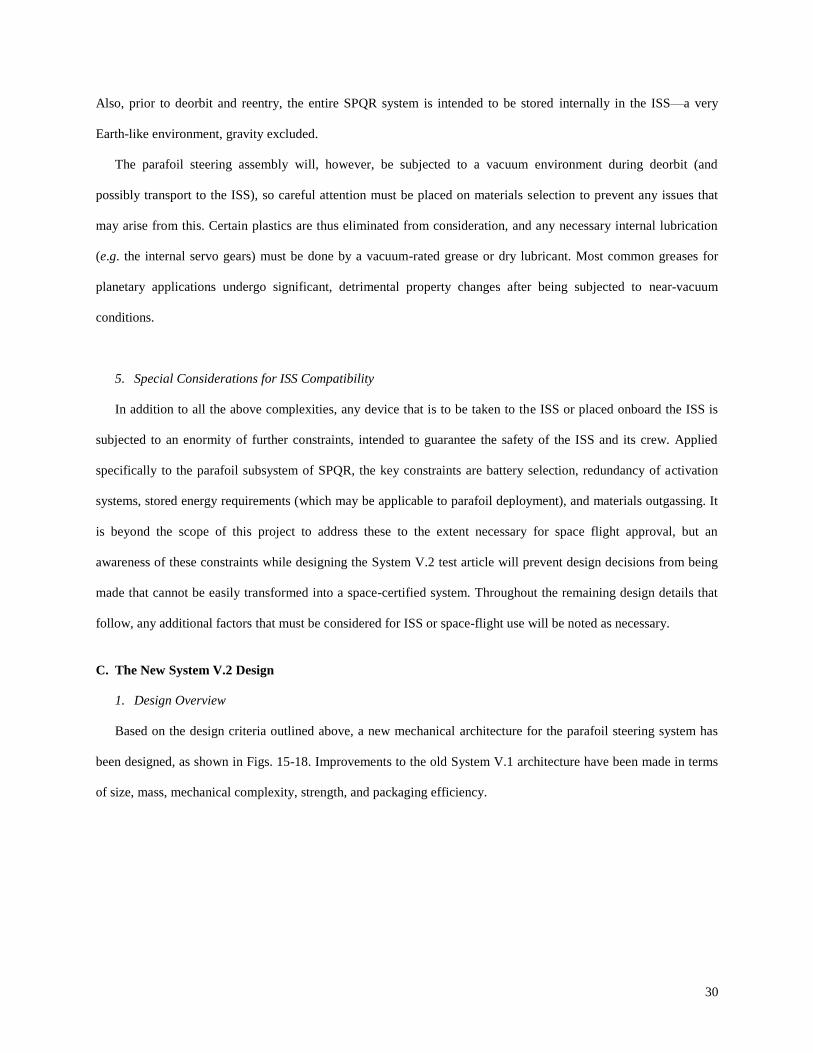
Based on the design criteria outlined above, a new mechanical architecture for the parafoil steering system has
been designed, as shown in Figs. 15-18. Improvements to the old System V.1 architecture have been made in terms
of size, mass, mechanical complexity, strength, and packaging efficiency.
31
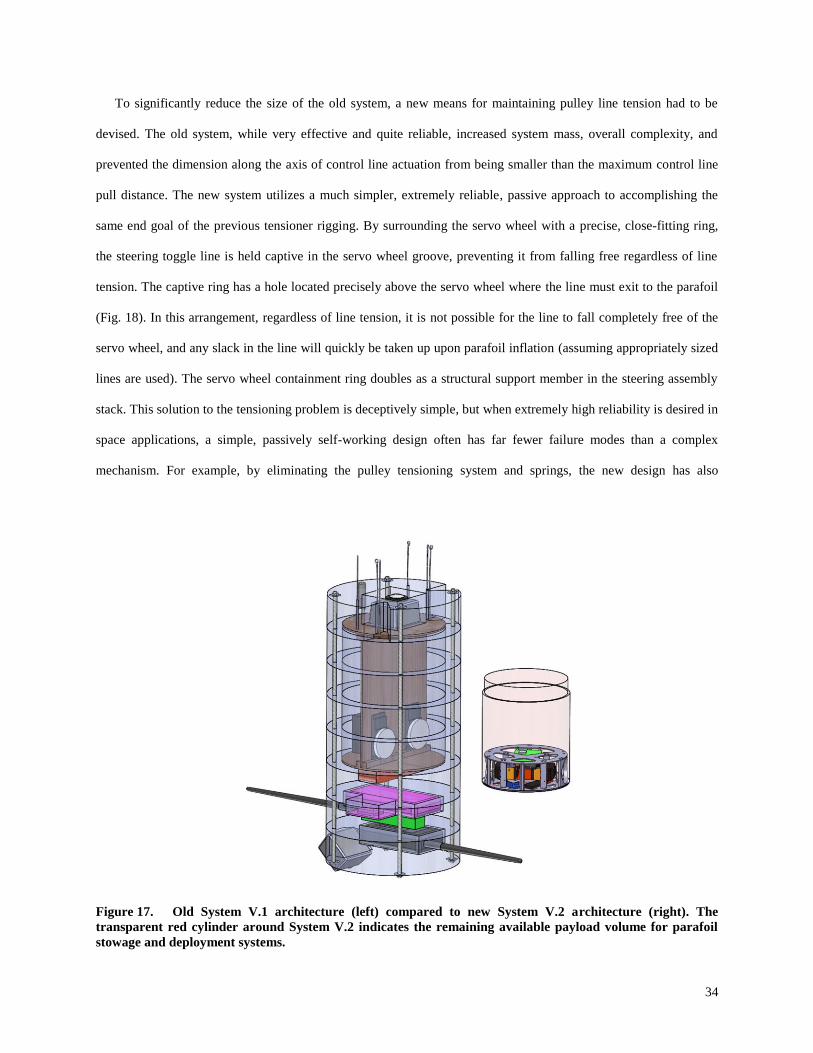
Figure 17 shows the old architecture compared to the new system to indicate a sense of scale. The new system is
volumetrically compatible with the PCTCU containment volume, while still maintaining the majority of the
compartment’s volume for parafoil stowage and deployment systems. Regard has been given to minimizing the
mechanical complexity of the system, keeping fabrication as simple as possible, and maintaining high reliability
within the mechanical steering system.
Figure 15. New, miniaturized System V.2 steering control architecture.
4.86 cm
(1.91 in)
Dia. 13.81 cm
(5.44 in)
32
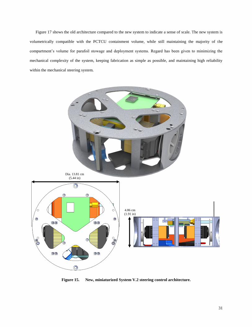
Figure 16. New, miniaturized System V.2 steering control system architecture (exploded view).
33
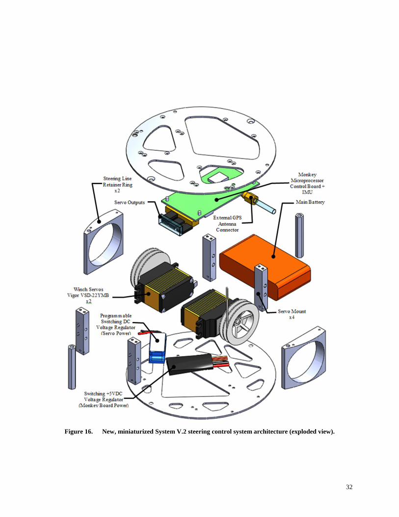
2. Design Improvements: Size, Mass, and Elimination of Line Tensioning System
Significant reduction in size was achieved through several means: minimizing empty space in the device;
selection of smaller servos while maintaining equivalent performance capability; converting structures to a
horizontal stacked deck configuration instead of the previous, volumetrically-inefficient vertical deck; and the
complete elimination of the pulley tensioning system.
Table 1 gives a component breakdown of total system mass for both the old and new system architecture. The
primary mass savings are gained through selection of new servos, and less inert structural mass (which included the
pulley tensioning system and all associated hardware in the old design). These improvements have resulted in a
considerable 87% reduction in system volume, and a 39% reduction in overall system mass for the parafoil steering
system mechanics.
Table 1. Mass and power breakdown for System V.1 (bottom) and System V.2 (top) components.
34
To significantly reduce the size of the old system, a new means for maintaining pulley line tension had to be
devised. The old system, while very effective and quite reliable, increased system mass, overall complexity, and
prevented the dimension along the axis of control line actuation from being smaller than the maximum control line
pull distance. The new system utilizes a much simpler, extremely reliable, passive approach to accomplishing the
same end goal of the previous tensioner rigging. By surrounding the servo wheel with a precise, close-fitting ring,
the steering toggle line is held captive in the servo wheel groove, preventing it from falling free regardless of line
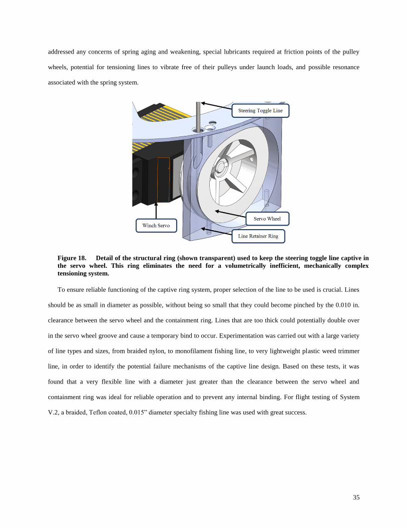
tension. The captive ring has a hole located precisely above the servo wheel where the line must exit to the parafoil
(Fig. 18). In this arrangement, regardless of line tension, it is not possible for the line to fall completely free of the
servo wheel, and any slack in the line will quickly be taken up upon parafoil inflation (assuming appropriately sized
lines are used). The servo wheel containment ring doubles as a structural support member in the steering assembly
stack. This solution to the tensioning problem is deceptively simple, but when extremely high reliability is desired in
space applications, a simple, passively self-working design often has far fewer failure modes than a complex
mechanism. For example, by eliminating the pulley tensioning system and springs, the new design has also
Figure 17. Old System V.1 architecture (left) compared to new System V.2 architecture (right). The
transparent red cylinder around System V.2 indicates the remaining available payload volume for parafoil
stowage and deployment systems.
35
addressed any concerns of spring aging and weakening, special lubricants required at friction points of the pulley
wheels, potential for tensioning lines to vibrate free of their pulleys under launch loads, and possible resonance
associated with the spring system.
To ensure reliable functioning of the captive ring system, proper selection of the line to be used is crucial. Lines
should be as small in diameter as possible, without being so small that they could become pinched by the 0.010 in.
clearance between the servo wheel and the containment ring. Lines that are too thick could potentially double over
in the servo wheel groove and cause a temporary bind to occur. Experimentation was carried out with a large variety
of line types and sizes, from braided nylon, to monofilament fishing line, to very lightweight plastic weed trimmer
line, in order to identify the potential failure mechanisms of the captive line design. Based on these tests, it was
found that a very flexible line with a diameter just greater than the clearance between the servo wheel and
containment ring was ideal for reliable operation and to prevent any internal binding. For flight testing of System
V.2, a braided, Teflon coated, 0.015” diameter specialty fishing line was used with great success.
Figure 18. Detail of the structural ring (shown transparent) used to keep the steering toggle line captive in
the servo wheel. This ring eliminates the need for a volumetrically inefficient, mechanically complex
tensioning system.
36
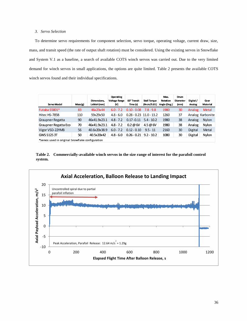
3. Servo Selection
To determine servo requirements for component selection, servo torque, operating voltage, current draw, size,
mass, and transit speed (the rate of output shaft rotation) must be considered. Using the existing servos in Snowflake
and System V.1 as a baseline, a search of available COTS winch servos was carried out. Due to the very limited
demand for winch servos in small applications, the options are quite limited. Table 2 presents the available COTS
winch servos found and their individual specifications.
Table 2. Commercially-available winch servos in the size range of interest for the parafoil control
system.
-10
-5
0
5
10
15
20
0 200 400 600 800 1000 1200
Axi
al P
aylo
ad A
cce
lera
tio
n, m
/s2
Elapsed Flight Time After Balloon Release, s
Axial Acceleration, Balloon Release to Landing Impact
Uncontrolled spiral due to partial parafoil inflation
Peak Acceleration, Parafoil Release: 12.64 m/s2
= 1.29g
37
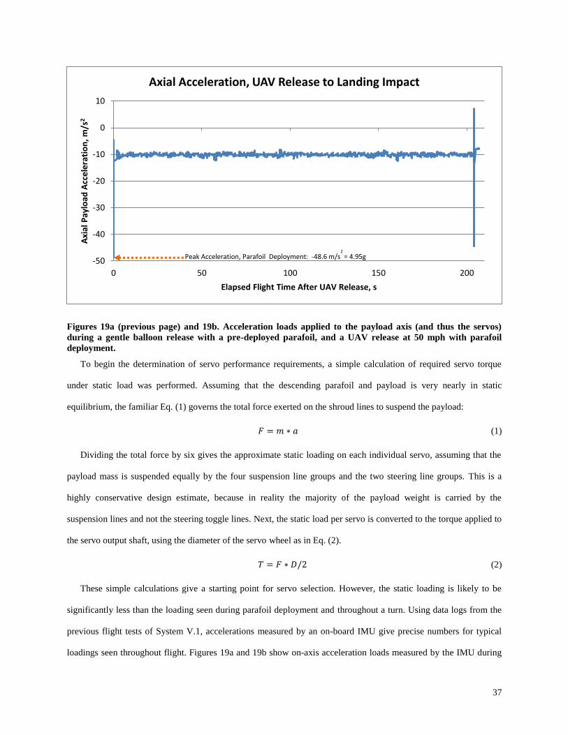
Figures 19a (previous page) and 19b. Acceleration loads applied to the payload axis (and thus the servos)
during a gentle balloon release with a pre-deployed parafoil, and a UAV release at 50 mph with parafoil
deployment.
To begin the determination of servo performance requirements, a simple calculation of required servo torque
under static load was performed. Assuming that the descending parafoil and payload is very nearly in static
equilibrium, the familiar Eq. (1) governs the total force exerted on the shroud lines to suspend the payload:
(1)
Dividing the total force by six gives the approximate static loading on each individual servo, assuming that the
payload mass is suspended equally by the four suspension line groups and the two steering line groups. This is a
highly conservative design estimate, because in reality the majority of the payload weight is carried by the
suspension lines and not the steering toggle lines. Next, the static load per servo is converted to the torque applied to
the servo output shaft, using the diameter of the servo wheel as in Eq. (2).
(2)
These simple calculations give a starting point for servo selection. However, the static loading is likely to be
significantly less than the loading seen during parafoil deployment and throughout a turn. Using data logs from the
previous flight tests of System V.1, accelerations measured by an on-board IMU give precise numbers for typical
loadings seen throughout flight. Figures 19a and 19b show on-axis acceleration loads measured by the IMU during
-50
-40
-30
-20
-10
0
10
0 50 100 150 200
Axi
al P
aylo
ad A
cce
lera
tio
n, m
/s2
Elapsed Flight Time After UAV Release, s
Axial Acceleration, UAV Release to Landing Impact
Peak Acceleration, Parafoil Deployment: -48.6 m/s2
= 4.95g
38
both a UAV flight test (where the parafoil was deployed at a velocity of approx. 50 mph) as well as a balloon drop.
Some of the data represents nominal flight conditions, while other data points were obtained in violent, high-
angular-velocity tumbles with a collapsed parafoil. Using this data, bounds can be placed on expected acceleration
loads in both normal flight as well as maximum stressing conditions. Finally, these acceleration loads can be applied
to the static load calculated above to determine reasonable design margin for servo capability.
The servo transit speed also plays an important role in system performance, but the associated requirement is
more difficult to quantify. In essence, the servo must respond quickly enough to command inputs to initiate a turn
without creating such a lag in response time that the guidance algorithm cannot properly compensate. A faster servo
will be beneficial for greater turning authority in flight and in final landing corrections. To complicate matters, the
parafoil-payload system also has an inherent control latency of its own. When the steering toggle line is first pulled,
there is a slight delay between the deformation of the parafoil and the actual initiation of the turn. The parafoil then
begins its turn, but the non-rigid connection to the payload through the shroud lines causes a delayed rotation of the
payload as the lines twist and then unload. Depending on the attitude determination scheme used, this can be more
or less of a problem. For example, a magnetometer serving as a compass will sense only the orientation of the
suspended payload, so it will not “see” a response to a commanded turn until the twisting of the shroud lines
overcomes the rotational inertia of the payload, causing it to turn as well. Alternatively, a GPS-based attitude
determination will calculate heading based on translation of the payload rather than magnetic field alignment, so the
flight control algorithm will be blind to any twisting of the payload beneath the parafoil.
The diameter of the servo wheel factors directly into the servo transit time, because a larger wheel will pull more
line for a given angular displacement, but requires greater torque to do so. Using the original servos utilized in the
Snowflake system as a baseline, the servo transit times and wheel diameters are presented in Table 2 for the
different servos considered. Because the servos all have similarly sized wheels, it can be assumed that any servo
with an equivalent transit time to the baseline servo will perform acceptably in this application, because the
Snowflake steering algorithm has already been proven effective at this response rate. The complexities of tuning the
new steering control system to the software are discussed in greater detail in Section VI: Flight Software
Development.
The final key considerations in servo selection are operating voltage and power consumption. This is addressed
in the next section, V: Electronics System Design. Based on all of the above, the Vigor VSD-22YMB servos were
39
chosen due to their small size, comparatively light weight, high torque, acceptable power consumption, metal gear
train, and impressive transit speed.
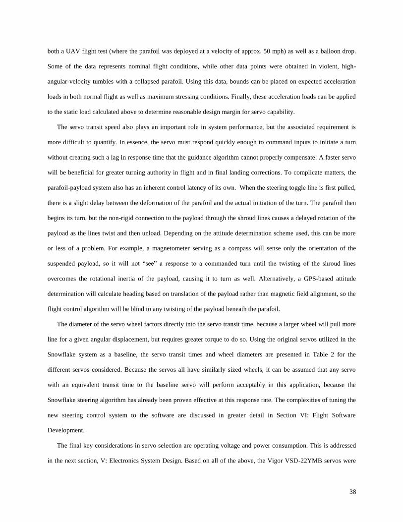
4. Structural Design
The structural components of System V.2 have been kept as simple and minimal as possible. The entire
structural assembly consists of only 10 major parts total, and of these ten parts, only 4 are unique. With a mass of
only 55 g, the structural assembly provides the backbone that supports all the components of the steering system
while contributing minimal weight. The design utilizes two circular discs of 0.063” aluminum, which are joined
together at 8 points distributed across their faces. The structure is extremely strong and rigid, and more than
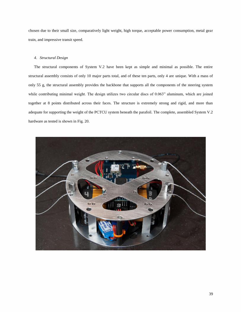
adequate for supporting the weight of the PCTCU system beneath the parafoil. The complete, assembled System V.2
hardware as tested is shown in Fig. 20.
40
Figures 20a and b (previous and current page). The complete System V.2 control hardware, after fabrication
and assembly.
41
V. System V.2 Electronics System Design
A. Design Context
The electronics system for the parafoil steering system has very few individual components, consisting of the
main battery, two DC voltage regulators (one for processor board power and one for dedicated servo power), a
control system microprocessor board, and two servos. A distinction should be made at this point between the System
V.2 design (as presented in this work) versus a flight-ready, space-worthy electronics system. For the former, a
multi-function microprocessor board with an integrated IMU provides the complete system intelligence, but in
actuality some aspects of the board’s capabilities are overkill for this application, and an even smaller custom
system could be designed with more specialized electronics. For a spaceflight-ready design, the electronics systems
and software algorithms would have to undergo very rigorous testing to guarantee reliability and performance. Also,
if smaller electronics boards were implemented, redundant processing systems could be utilized to ensure a greater
degree of reliability.
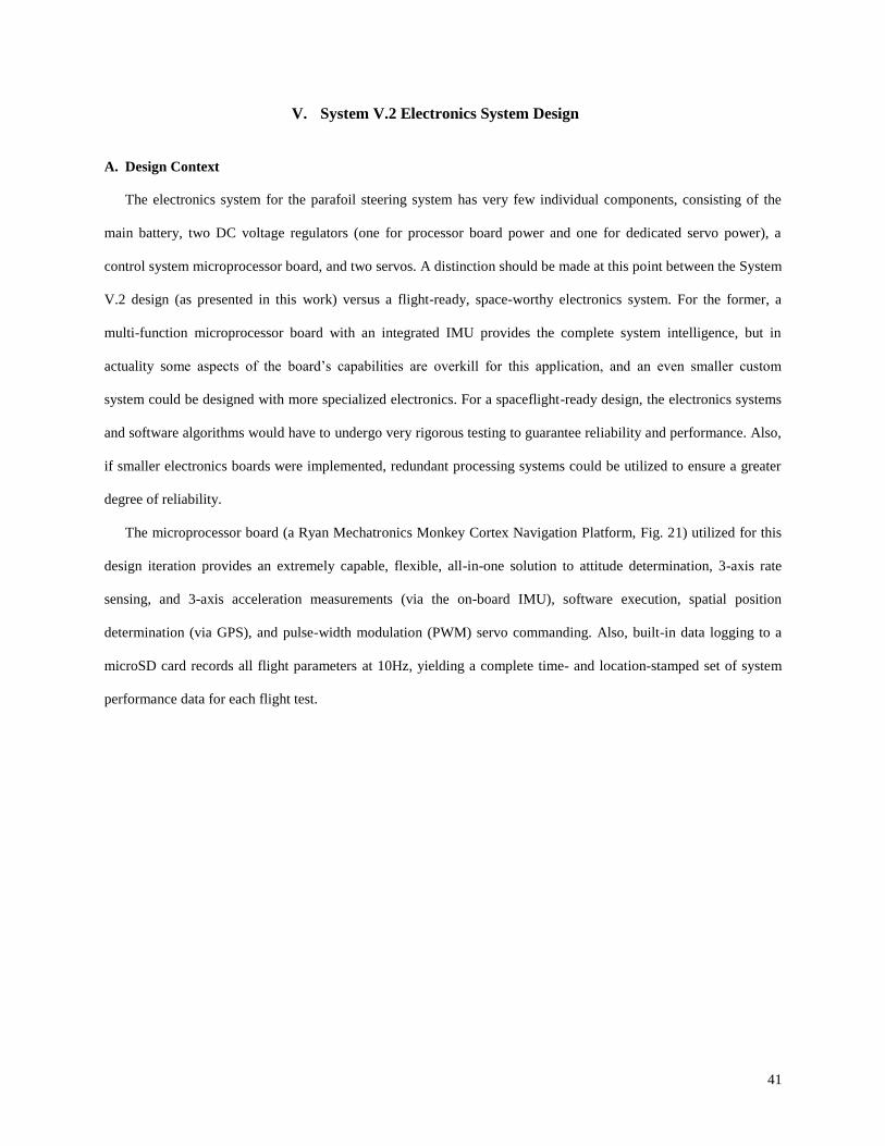
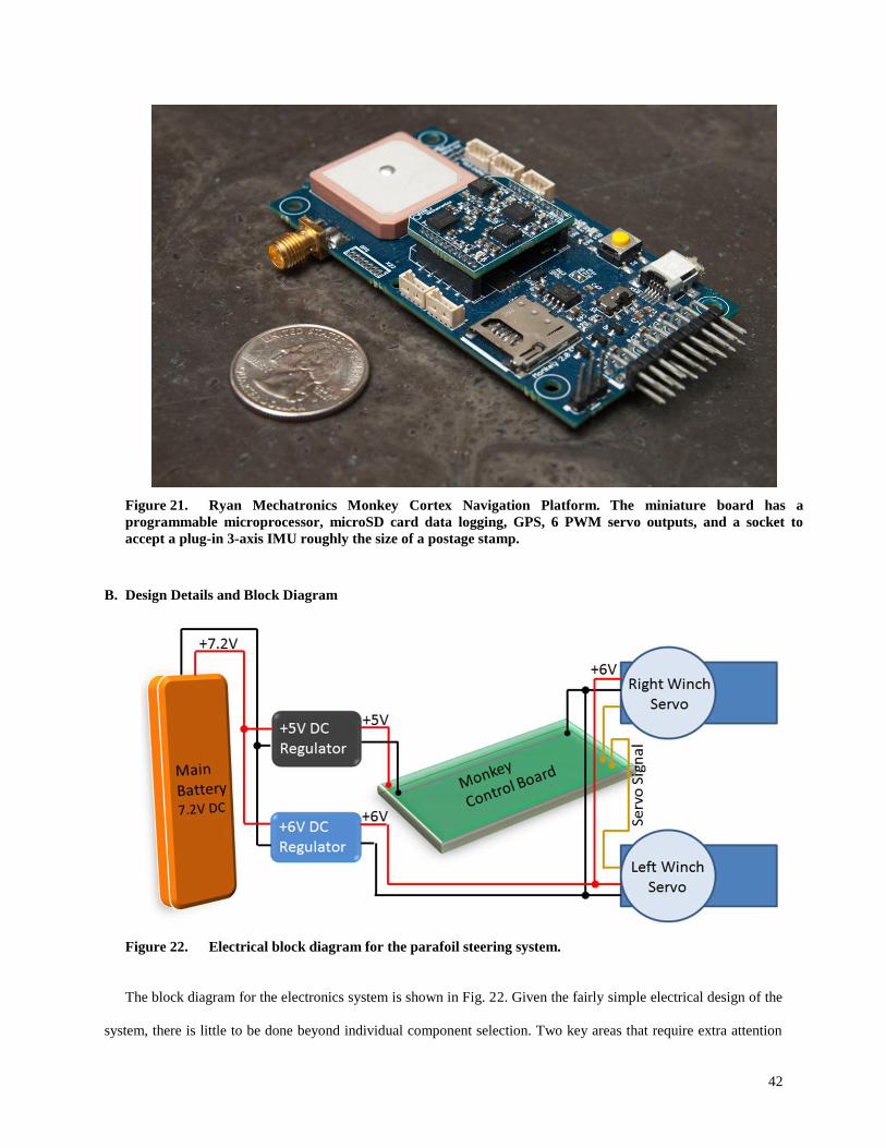
The microprocessor board (a Ryan Mechatronics Monkey Cortex Navigation Platform, Fig. 21) utilized for this
design iteration provides an extremely capable, flexible, all-in-one solution to attitude determination, 3-axis rate
sensing, and 3-axis acceleration measurements (via the on-board IMU), software execution, spatial position
determination (via GPS), and pulse-width modulation (PWM) servo commanding. Also, built-in data logging to a
microSD card records all flight parameters at 10Hz, yielding a complete time- and location-stamped set of system
performance data for each flight test.
42
B. Design Details and Block Diagram
The block diagram for the electronics system is shown in Fig. 22. Given the fairly simple electrical design of the
system, there is little to be done beyond individual component selection. Two key areas that require extra attention
Figure 21. Ryan Mechatronics Monkey Cortex Navigation Platform.
The miniature board has a
programmable microprocessor, microSD card data logging, GPS, 6 PWM servo outputs, and a socket to
accept a plug-in 3-axis IMU roughly the size of a postage stamp.
Figure 22. Electrical block diagram for the parafoil steering system.
43
are battery selection and power distribution. The battery is the heaviest individual component of the entire steering
system, so it is important to choose a battery with sufficient capacity to power the entirety of the flight (with
appropriate design margin) without adding extra “dead weight” to the system. Also, the nominal voltage of the
battery must be greater than the required input voltage of any of the individual components, because the switching-
mode voltage regulators chosen for System V.2 cannot increase voltage beyond the battery input voltage. For a
given battery chemistry, pack voltage is determined by the number of cells in series in the battery pack.
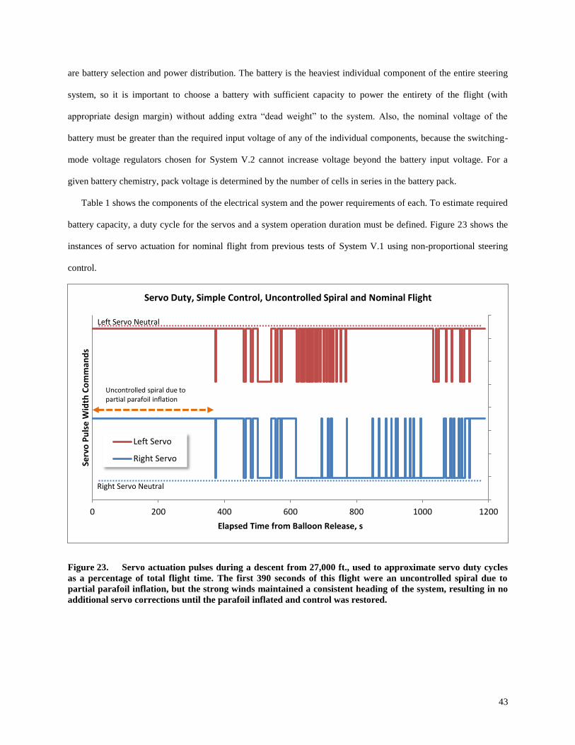
Table 1 shows the components of the electrical system and the power requirements of each. To estimate required
battery capacity, a duty cycle for the servos and a system operation duration must be defined. Figure 23 shows the
instances of servo actuation for nominal flight from previous tests of System V.1 using non-proportional steering
control.
Figure 23. Servo actuation pulses during a descent from 27,000 ft., used to approximate servo duty cycles
as a percentage of total flight time. The first 390 seconds of this flight were an uncontrolled spiral due to
partial parafoil inflation, but the strong winds maintained a consistent heading of the system, resulting in no
additional servo corrections until the parafoil inflated and control was restored.
0 200 400 600 800 1000 1200
Serv
o P
uls
e W
idth
Co
mm
and
s
Elapsed Time from Balloon Release, s
Servo Duty, Simple Control, Uncontrolled Spiral and Nominal Flight
Left Servo
Right Servo
Uncontrolled spiral due to partial parafoil inflation
Right Servo Neutral
Left Servo Neutral
44
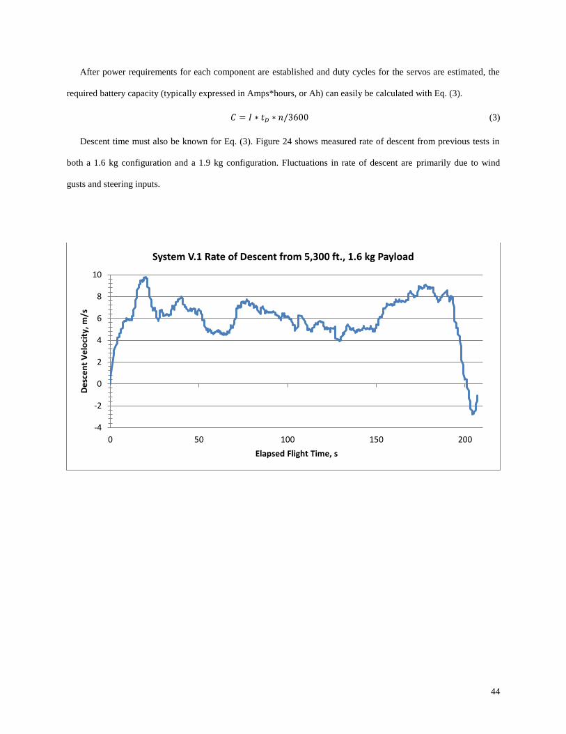
After power requirements for each component are established and duty cycles for the servos are estimated, the
required battery capacity (typically expressed in Amps*hours, or Ah) can easily be calculated with Eq. (3).
(3)
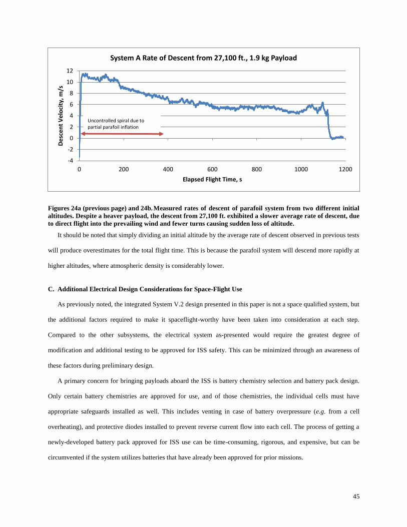
Descent time must also be known for Eq. (3). Figure 24 shows measured rate of descent from previous tests in
both a 1.6 kg configuration and a 1.9 kg configuration. Fluctuations in rate of descent are primarily due to wind
gusts and steering inputs.
-4
-2
0
2
4
6
8
10
0 50 100 150 200
De
sce
nt
Ve
loci
ty, m
/s
Elapsed Flight Time, s
System V.1 Rate of Descent from 5,300 ft., 1.6 kg Payload
45
Figures 24a (previous page) and 24b. Measured rates of descent of parafoil system from two different initial
altitudes. Despite a heaver payload, the descent from 27,100 ft. exhibited a slower average rate of descent, due
to direct flight into the prevailing wind and fewer turns causing sudden loss of altitude.
It should be noted that simply dividing an initial altitude by the average rate of descent observed in previous tests
will produce overestimates for the total flight time. This is because the parafoil system will descend more rapidly at
higher altitudes, where atmospheric density is considerably lower.
C. Additional Electrical Design Considerations for Space-Flight Use
As previously noted, the integrated System V.2 design presented in this paper is not a space qualified system, but
the additional factors required to make it spaceflight-worthy have been taken into consideration at each step.
Compared to the other subsystems, the electrical system as-presented would require the greatest degree of
modification and additional testing to be approved for ISS safety. This can be minimized through an awareness of
these factors during preliminary design.
A primary concern for bringing payloads aboard the ISS is battery chemistry selection and battery pack design.
Only certain battery chemistries are approved for use, and of those chemistries, the individual cells must have
appropriate safeguards installed as well. This includes venting in case of battery overpressure (e.g. from a cell
overheating), and protective diodes installed to prevent reverse current flow into each cell. The process of getting a
newly-developed battery pack approved for ISS use can be time-consuming, rigorous, and expensive, but can be
circumvented if the system utilizes batteries that have already been approved for prior missions.
-4
-2
0
2
4
6
8
10
12
0 200 400 600 800 1000 1200
De
sce
nt
Ve
loci
ty, m
/s
Elapsed Flight Time, s
System A Rate of Descent from 27,100 ft., 1.9 kg Payload
Uncontrolled spiral due to partial parafoil inflation
46
Another consideration that poses great difficulty on-board the ISS is battery charging—for most applications,
especially ones intended to be as simple as SPQR, charging onboard the ISS should be avoided at all costs. For the
parafoil return system (and indeed the entire SPQR system), primary (non-rechargeable) cells are preferable for
several reasons: the approval process for ISS use is greatly simplified if charging is not required; primary cells have
a much lower rate of self-discharge in storage compared to rechargeable cells; primary cells offer excellent energy
density; electronics system design is simplified without including a charging circuit; solar cells for space
applications are expensive; and, the short operational duration and modest power consumption of the SPQR and
parafoil systems pose no need for in-flight solar recharging.
If any of the electronics of the parafoil system were in a powered-on state aboard the ISS, extensive testing of the
electrical components and control board would be required to satisfy safety requirements. However, if the electrical
systems can be guaranteed to be completely isolated from battery power at any time prior to release from the ISS,
this safety concern is eliminated. For this reason, the parafoil system will utilize redundant activation switches in
series with the battery, thus requiring both of the switches to be closed before the electronics of the parafoil system
will be powered-on. One of the switches will be activated by removal of a remove-before-flight pin (common in
such applications) prior to the jettison of the SPQR system from the ISS, and the second switch will be activated just
prior to reentry, when the reentry vehicle is separated from the SPQR de-orbit system.
Other common spaceflight concerns for electronics include radiation hardening, thermal and vacuum
environments, and tolerance to shock and vibrational loads. The short lifetime in-orbit (on the order of several days),
combined with the containment inside the PCTCU structure negates the need for radiation hardened components,
particularly if redundant processing boards are utilized. The systems must undergo thermal vacuum testing for
space-worthiness, and shock and vibration testing as well. The shock and vibrational loads encountered by the
system in actual use are likely to be very modest, because the SPQR device would likely be carried as a “soft-stow”
item aboard an ISS resupply vehicle.
The operational duration of the parafoil system for ISS payload return and the previous System V.1 balloon tests
will differ very little in terms of total time powered-on and time to payload recovery. Both the full-fledged SPQR
system and the SystemV.1 balloon-test platform begin their mission phases at comparable altitudes, and the actual
ISS return scenario will have greater resources focused on payload trajectory, tracking and recovery than an amateur
balloon test. For these reasons, it is reasonable to expect that total power requirements for System V.2 and the actual

47
SPQR parafoil return system will be similar, and the battery’s mass and volume accommodations will be compatible
for both (assuming the SPQR device has an independent battery for the parafoil system, which has yet to be defined
in the larger SPQR concept).
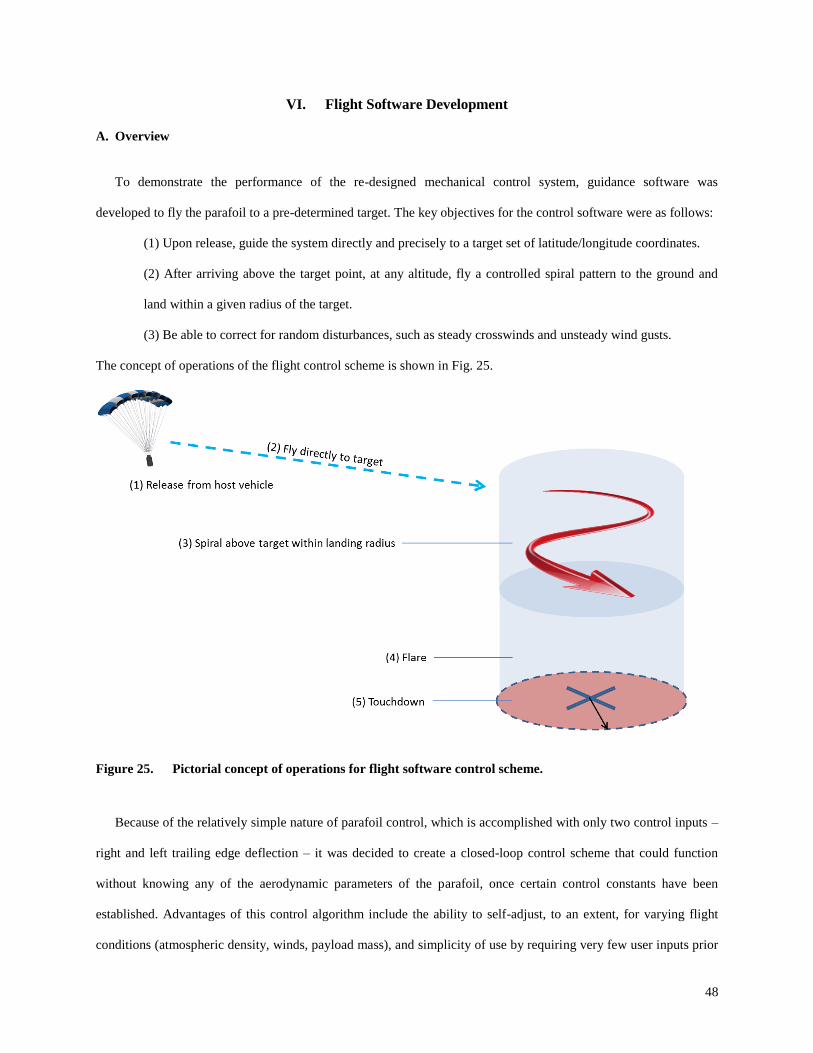
48
VI. Flight Software Development
A. Overview
To demonstrate the performance of the re-designed mechanical control system, guidance software was
developed to fly the parafoil to a pre-determined target. The key objectives for the control software were as follows:
(1) Upon release, guide the system directly and precisely to a target set of latitude/longitude coordinates.
(2) After arriving above the target point, at any altitude, fly a controlled spiral pattern to the ground and
land within a given radius of the target.
(3) Be able to correct for random disturbances, such as steady crosswinds and unsteady wind gusts.
The concept of operations of the flight control scheme is shown in Fig. 25.
Figure 25. Pictorial concept of operations for flight software control scheme.
Because of the relatively simple nature of parafoil control, which is accomplished with only two control inputs –
right and left trailing edge deflection – it was decided to create a closed-loop control scheme that could function
without knowing any of the aerodynamic parameters of the parafoil, once certain control constants have been
established. Advantages of this control algorithm include the ability to self-adjust, to an extent, for varying flight
conditions (atmospheric density, winds, payload mass), and simplicity of use by requiring very few user inputs prior
49
to flight. With the software as developed, the parafoil system can be deployed at any point around the world with a
clear view to several GPS satellites, and it will attempt to fly directly to a target set of coordinates until it either
arrives at the target or runs out of altitude and lands, whichever occurs first.
The control software is programmed in the C programming language, and code snippets are presented below in
with appropriate descriptions of what each set of code does. The full software code can be found in its entirety in
Appendix A.
B. Software Control Algorithm Flow Charts
The flow charts for the software guidance routine are shown on the following pages in Figs. 26-31. A detailed
description of the individual software processes is given in Part C: Detailed Description of Control Methodology.
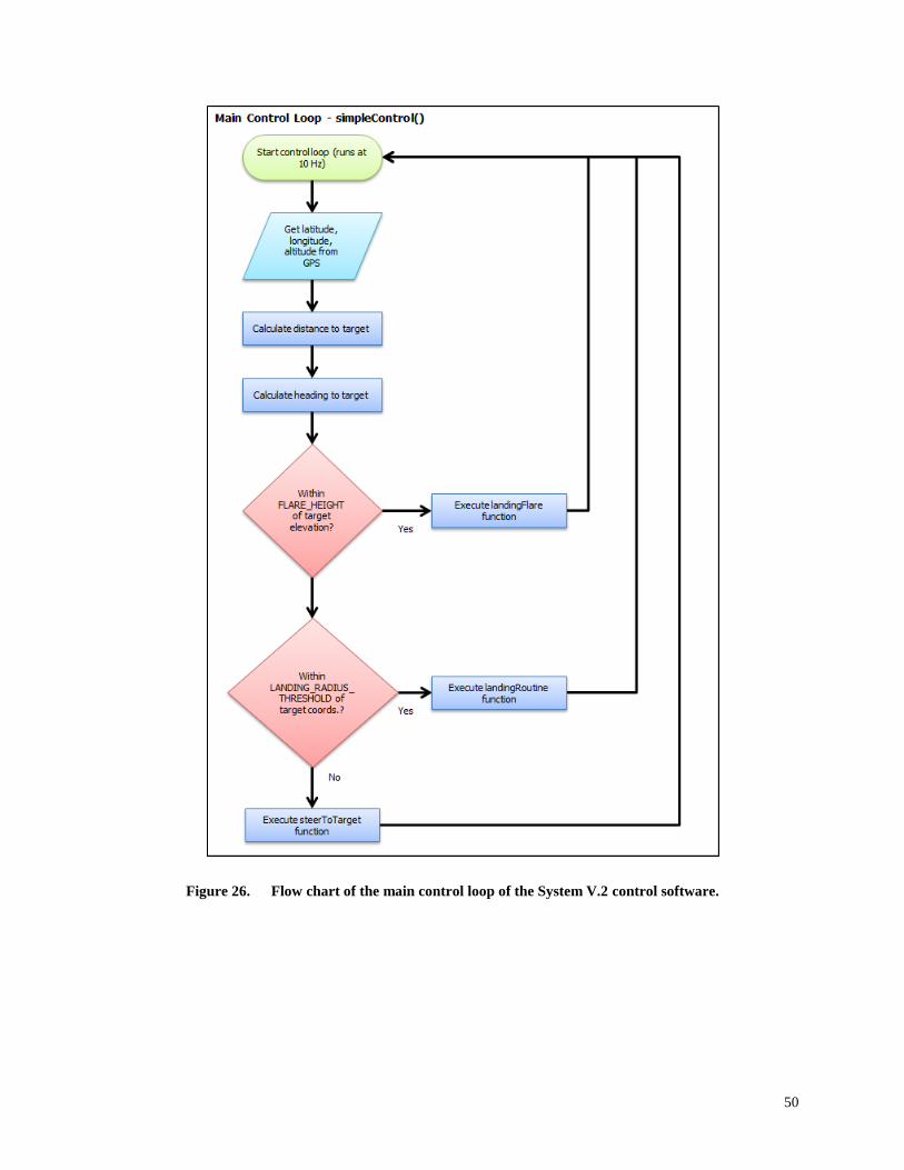
50
Figure 26. Flow chart of the main control loop of the System V.2 control software.
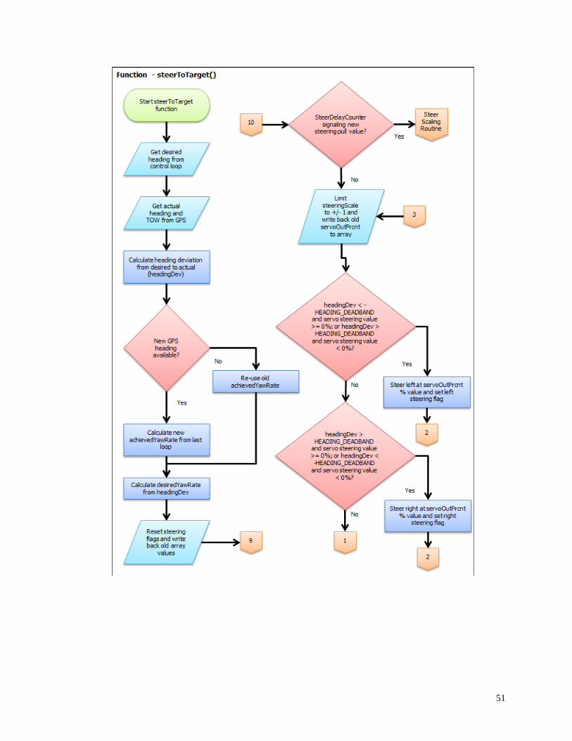
51
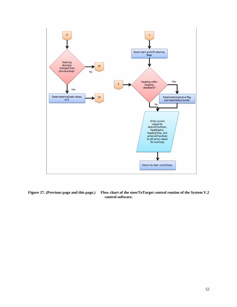
52
Figure 27. (Previous page and this page.) Flow chart of the steerToTarget control routine of the System V.2
control software.
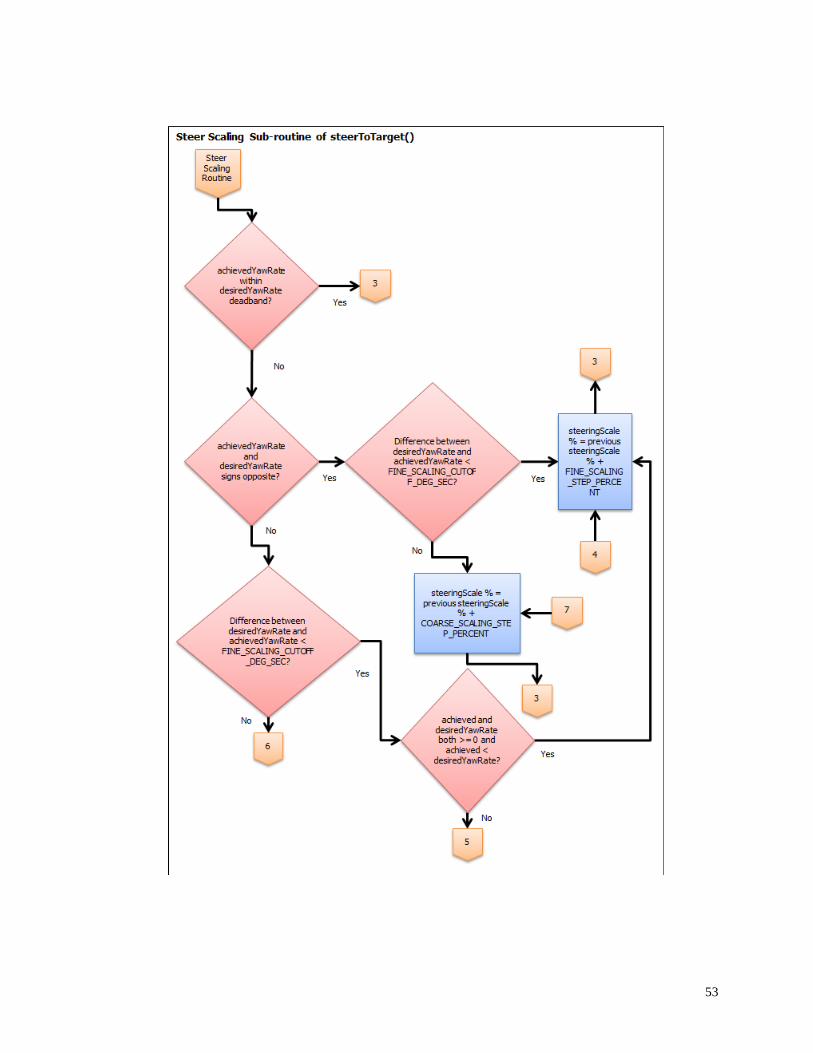
53
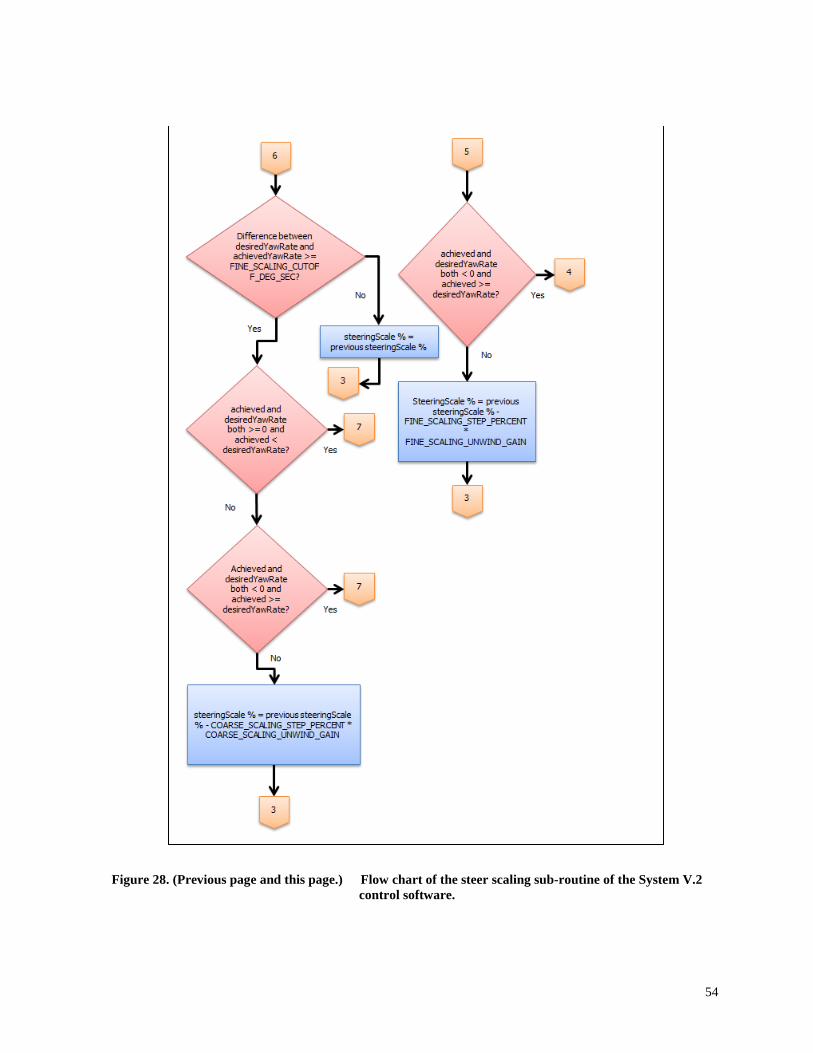
54
Figure 28. (Previous page and this page.) Flow chart of the steer scaling sub-routine of the System V.2
control software.
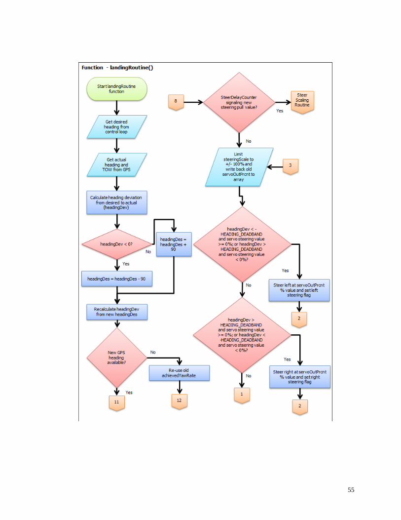
55
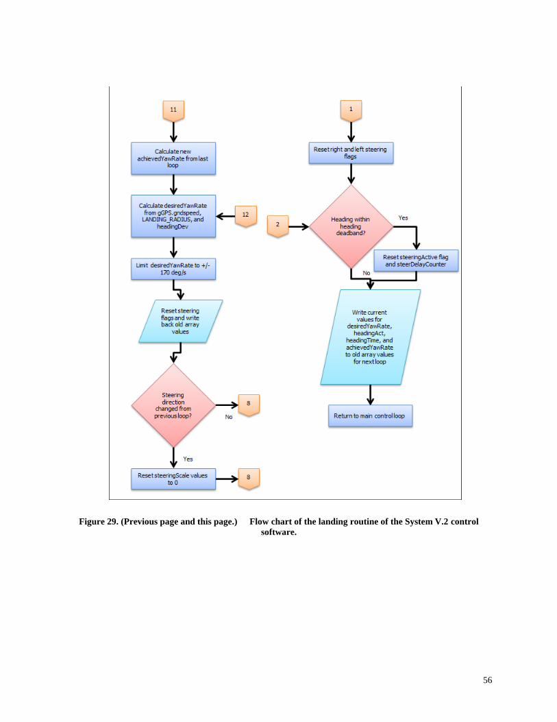
56
Figure 29. (Previous page and this page.) Flow chart of the landing routine of the System V.2 control
software.
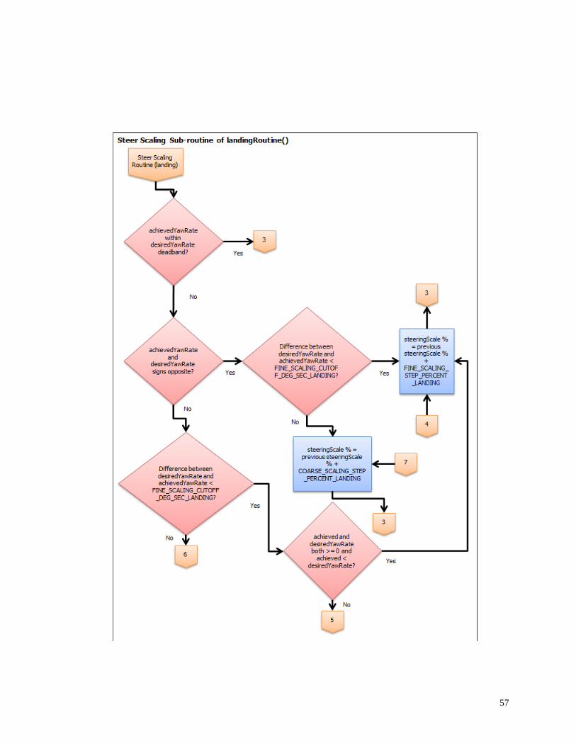
57
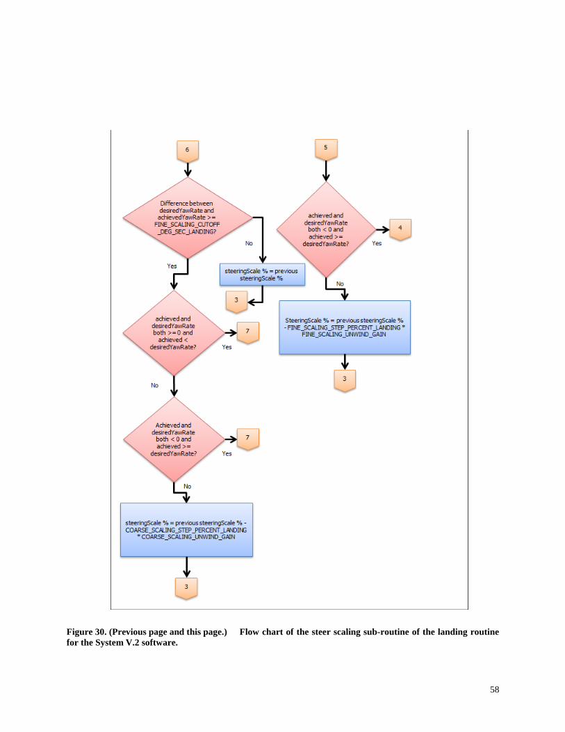
58
Figure 30. (Previous page and this page.) Flow chart of the steer scaling sub-routine of the landing routine
for the System V.2 software.
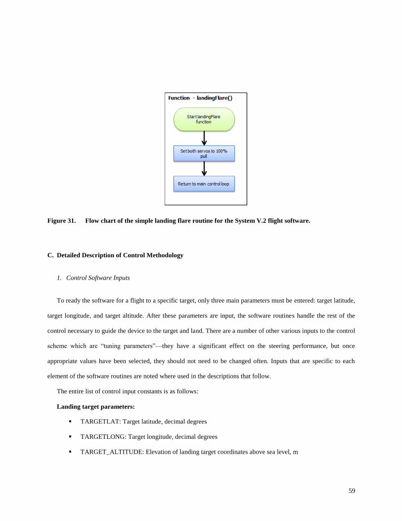
59
Figure 31. Flow chart of the simple landing flare routine for the System V.2 flight software.
C. Detailed Description of Control Methodology
1. Control Software Inputs
To ready the software for a flight to a specific target, only three main parameters must be entered: target latitude,
target longitude, and target altitude. After these parameters are input, the software routines handle the rest of the
control necessary to guide the device to the target and land. There are a number of other various inputs to the control
scheme which are “tuning parameters”—they have a significant effect on the steering performance, but once
appropriate values have been selected, they should not need to be changed often. Inputs that are specific to each
element of the software routines are noted where used in the descriptions that follow.
The entire list of control input constants is as follows:
Landing target parameters:
TARGETLAT: Target latitude, decimal degrees
TARGETLONG: Target longitude, decimal degrees
TARGET_ALTITUDE: Elevation of landing target coordinates above sea level, m
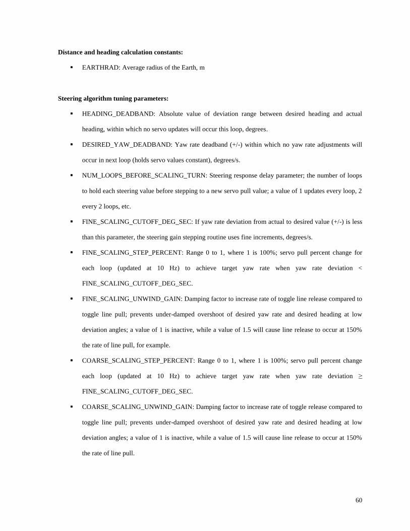
60
Distance and heading calculation constants:
EARTHRAD: Average radius of the Earth, m
Steering algorithm tuning parameters:
HEADING_DEADBAND: Absolute value of deviation range between desired heading and actual
heading, within which no servo updates will occur this loop, degrees.
DESIRED_YAW_DEADBAND: Yaw rate deadband (+/-) within which no yaw rate adjustments will
occur in next loop (holds servo values constant), degrees/s.
NUM_LOOPS_BEFORE_SCALING_TURN: Steering response delay parameter; the number of loops
to hold each steering value before stepping to a new servo pull value; a value of 1 updates every loop, 2
every 2 loops, etc.
FINE_SCALING_CUTOFF_DEG_SEC: If yaw rate deviation from actual to desired value (+/-) is less
than this parameter, the steering gain stepping routine uses fine increments, degrees/s.
FINE_SCALING_STEP_PERCENT: Range 0 to 1, where 1 is 100%; servo pull percent change for
each loop (updated at 10 Hz) to achieve target yaw rate when yaw rate deviation <
FINE_SCALING_CUTOFF_DEG_SEC.
FINE_SCALING_UNWIND_GAIN: Damping factor to increase rate of toggle line release compared to
toggle line pull; prevents under-damped overshoot of desired yaw rate and desired heading at low
deviation angles; a value of 1 is inactive, while a value of 1.5 will cause line release to occur at 150%
the rate of line pull, for example.
COARSE_SCALING_STEP_PERCENT: Range 0 to 1, where 1 is 100%; servo pull percent change
each loop (updated at 10 Hz) to achieve target yaw rate when yaw rate deviation ≥
FINE_SCALING_CUTOFF_DEG_SEC.
COARSE_SCALING_UNWIND_GAIN: Damping factor to increase rate of toggle release compared to
toggle line pull; prevents under-damped overshoot of desired yaw rate and desired heading at low
deviation angles; a value of 1 is inactive, while a value of 1.5 will cause line release to occur at 150%
the rate of line pull.
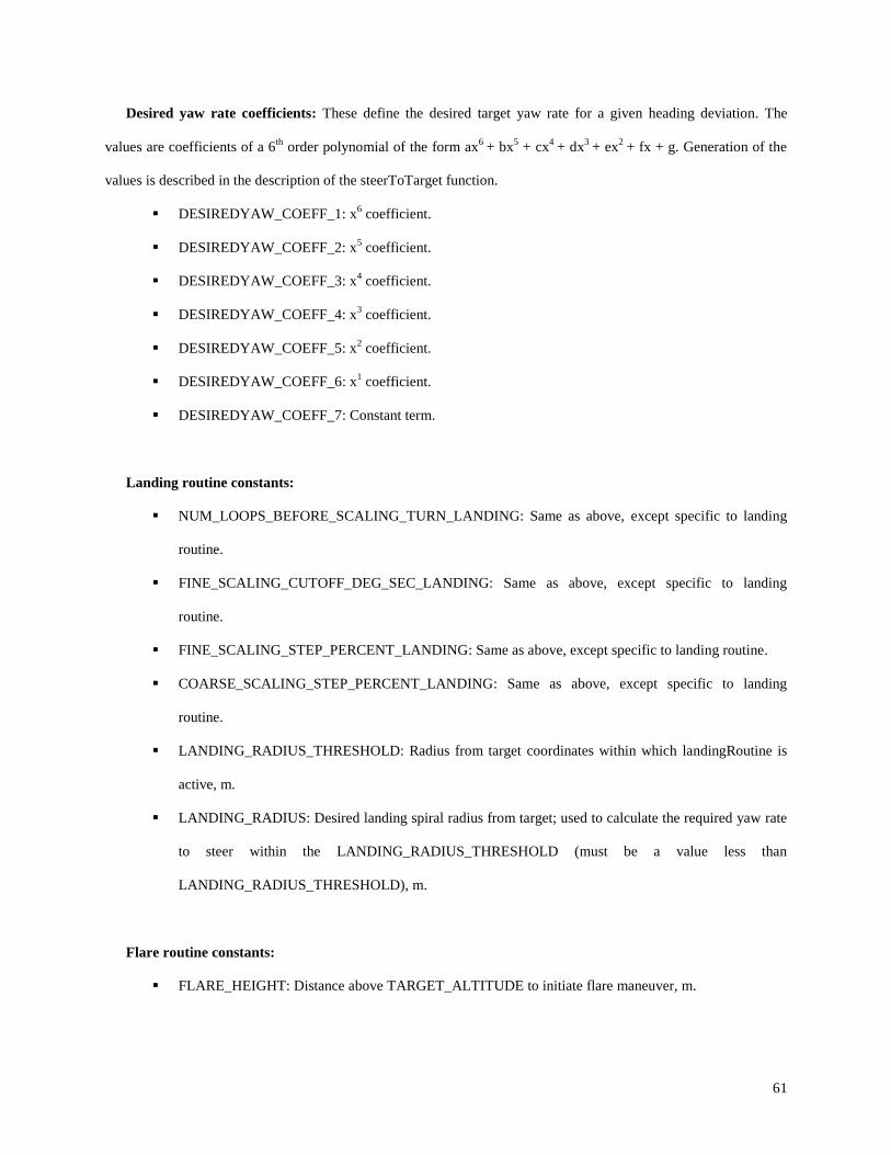
61
Desired yaw rate coefficients: These define the desired target yaw rate for a given heading deviation. The
values are coefficients of a 6th
order polynomial of the form ax6
+ bx5 + cx
4 + dx
3 + ex
2 + fx + g. Generation of the
values is described in the description of the steerToTarget function.
DESIREDYAW_COEFF_1: x6 coefficient.
DESIREDYAW_COEFF_2: x5 coefficient.
DESIREDYAW_COEFF_3: x4 coefficient.
DESIREDYAW_COEFF_4: x3 coefficient.
DESIREDYAW_COEFF_5: x2 coefficient.
DESIREDYAW_COEFF_6: x1 coefficient.
DESIREDYAW_COEFF_7: Constant term.
Landing routine constants:
NUM_LOOPS_BEFORE_SCALING_TURN_LANDING: Same as above, except specific to landing
routine.
FINE_SCALING_CUTOFF_DEG_SEC_LANDING: Same as above, except specific to landing
routine.
FINE_SCALING_STEP_PERCENT_LANDING: Same as above, except specific to landing routine.
COARSE_SCALING_STEP_PERCENT_LANDING: Same as above, except specific to landing
routine.
LANDING_RADIUS_THRESHOLD: Radius from target coordinates within which landingRoutine is
active, m.
LANDING_RADIUS: Desired landing spiral radius from target; used to calculate the required yaw rate
to steer within the LANDING_RADIUS_THRESHOLD (must be a value less than
LANDING_RADIUS_THRESHOLD), m.
Flare routine constants:
FLARE_HEIGHT: Distance above TARGET_ALTITUDE to initiate flare maneuver, m.
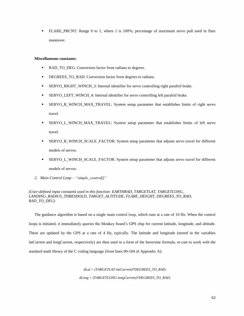
62
FLARE_PRCNT: Range 0 to 1, where 1 is 100%; percentage of maximum servo pull used in flare
maneuver.
Miscellaneous constants:
RAD_TO_DEG: Conversion factor from radians to degrees.
DEGREES_TO_RAD: Conversion factor from degrees to radians.
SERVO_RIGHT_WINCH_3: Internal identifier for servo controlling right parafoil brake.
SERVO_LEFT_WINCH_4: Internal identifier for servo controlling left parafoil brake.
SERVO_R_WINCH_MAX_TRAVEL: System setup parameter that establishes limits of right servo
travel.
SERVO_L_WINCH_MAX_TRAVEL: System setup parameter that establishes limits of left servo
travel.
SERVO_R_WINCH_SCALE_FACTOR: System setup parameter that adjusts servo travel for different
models of servos.
SERVO_L_WINCH_SCALE_FACTOR: System setup parameter that adjusts servo travel for different
models of servos.
2. Main Control Loop – “simple_control()”
(User-defined input constants used in this function: EARTHRAD, TARGETLAT, TARGETLONG,
LANDING_RADIUS_THRESHOLD, TARGET_ALTITUDE, FLARE_HEIGHT, DEGREES_TO_RAD,
RAD_TO_DEG)
The guidance algorithm is based on a single main control loop, which runs at a rate of 10 Hz. When the control
loops is initiated, it immediately queries the Monkey board’s GPS chip for current latitude, longitude, and altitude.
These are updated by the GPS at a rate of 4 Hz, typically. The latitude and longitude (stored in the variables
latCurrent and longCurrent, respectively) are then used in a form of the haversine formula, re-cast to work with the
standard math library of the C coding language (from lines 90-104 of Appendix A):
dLat = (TARGETLAT-latCurrent)*DEGREES_TO_RAD;
dLong = (TARGETLONG-longCurrent)*DEGREES_TO_RAD;
63
latCurrentRad = latCurrent*DEGREES_TO_RAD; //current latitude in radians
targetLatRad = TARGETLAT*DEGREES_TO_RAD; //current longitude in radians
aDist = sin(dLat/2) * sin(dLat/2) + sin(dLong/2) * sin(dLong/2) * cos(latCurrentRad) * cos(targetLatRad);
cDist = 2 * atan2(sqrt(aDist), sqrt(1-aDist));
distMag = EARTHRAD * cDist;
(4)
The output of the above expressions returns the magnitude of the great-circle distance from the parafoil system’s
current location to the target coordinates in meters. Next, the heading (0 to 360°) from the current position to the
target is calculated as follows, from lines 108-113 of the software C source file:
yHead = sin(dLong) * cos(targetLatRad);
xHead = cos(latCurrentRad)*sin(targetLatRad) -
sin(latCurrentRad)*cos(targetLatRad)*cos(dLong);
headingDes = atan2(yHead, xHead)*RAD_TO_DEG; //returns desired heading in degrees from -180 to 180
headingDes >= 0 ? (headingDesRnd = (int)(headingDes+0.5)) : (headingDesRnd = (int)(headingDes-0.5)); //rounds
headingDes for the modulo operator on next line
headingDes = (headingDesRnd+360) % 360; //uses headingDesRnd to return 0 <= int headingDes < 360
(5)
The variable headingDes is returned from the above code, which is the heading from 0 to 360° that the parafoil
system must fly to reach its target, where due north corresponds to 0° and heading degree values increase in a
clockwise direction.
With the calculation of the heading to the target and the distance to the target completed, the control loop reaches
a decision point with three possible outcomes:
(1) If the system’s altitude is less than TARGET_ALTITUDE + FLARE_HEIGHT, the landingFlare()
function is called.
(2) If the magnitude of the system’s distance from the target coordinates is less than
LANDING_RADIUS_THRESHOLD, the landingRoutine() function is called.
64
(3) Otherwise, the system is in normal flight toward the target, and the steerToTarget() function is called.
3. Nominal Flight Guidance Routine – “steerToTarget()”
(User-defined input constants used in this function: HEADING_DEADBAND, DESIREDYAW_COEFF[1-7],
NUM_LOOPS_BEFORE_SCALING_TURN, DESIRED_YAW_DEADBAND, SERVO_RIGHT_WINCH_3,
SERVO_LEFT_WINCH_4, SERVO_R_WINCH_MAX_TRAVEL, SERVO_L_WINCH_MAX_TRAVEL,
SERVO_R_WINCH_SCALE_FACTOR, SERVO_L_WINCH_SCALE_FACTOR, FINE_SCALING_UNWIND_GAIN,
COARSE_SCALING_UNWIND_GAIN, FINE_SCALING_STEP_PERCENT,
COARSE_SCALING_STEP_PERCENT, FINE_SCALING_CUTOFF_DEG_SEC)
If the parafoil system has not arrived within the landing radius threshold or reached the elevation to initiate
the landing flare, it is in the nominal flight phase. This phase is controlled by the function steerToTarget(). This
function is responsible for the calculation of all steering parameters and sends the commands to the servos to
execute control. The global variable headingDes (the desired heading from the current position to the target) is
passed from the main control loop, simple_control(), to steerToTarget().
Upon entering the function, the GPS is queried for system heading and the parameter TOW (time of week).
TOW is used rather than UTC time because the Monkey control board reports TOW in quarter-second resolution as
opposed to 1-second resolution of UTC time. This enables more frequent sampling and calculation of key control
parameters described below. The system heading and TOW values are stored in the array variables headingAct and
headingTime, respectively. For all array variables used in the control software, the leading value in the array
(position 0) is the value for the current control loop. The other values (in most cases the arrays store only two
values) are the values for the previous control loops. For example, headingAct[0] holds the value of the actual
heading determined in the current run of the control loop, and headingAct[1] holds the value of the same variable
that was used in the previous control loop. Because the steering algorithm relies on closed-loop system feedback,
these multi-value arrays are used to evaluate the response of previous commands and then adjust the current
commands accordingly.
The next step of the steerToTarget routine is the determination of heading deviation. The variable headingDev is
used to store the value of the heading deviation measured from the actual device heading to the desired heading. If
the heading difference from actual to desired is in a clockwise direction, the value of headingDev is positive, and
vice versa. headingDev is reported as a value ranging from -180° to +180°. The calculation of headingDev is found
in lines 185-193 of the complete software code in Appendix A.
65
Once headingDev is known, steerToTarget calculates an approximate yaw rate of the system from the previous
loop to the current loop (lines 199-209 in Appendix A). The value is not actually a yaw rate in the traditional sense,
because it is calculated based on the actual flight heading of the device in the previous loop and the flight heading in
the current loop. The value is stored in the two-value array variable achievedYawRate, and is found by dividing the
change in flight heading from the previous loop to the current loop by the time elapsed from the previous loop to
current loop. One nuance of this calculation is that the entire control loop routine is run at 10Hz to ensure smooth
servo stepping operation, but the GPS chip typically updates only at 0.25-second intervals. To prevent a calculation
of 0°/s yaw rates when the GPS value has not yet updated, a conditional test is included to ensure that a new value of
GPS heading exists before calculating a new achievedYawRate. The achievedYawRate is returned as a value of -
180°/s to +180°/s, due to a limitation of calculating it from the system heading. That is, if the system rotates 540°
from the previous loop to the current loop, it will look no different to the GPS-reported headings than if it rotated
180°, for example. For this reason, the yaw rates the parafoil system tries to achieve in turning are kept well below
this 180°/s threshold.
Despite the limitation of ±180°/s maximum resolution, utilizing the GPS heading for yaw rate determination
(rather than the on-board rate gyro from the Monkey board’s IMU) bears a distinct advantage that greatly simplifies
and improves efficiency of control calculations. In a parafoil-payload system, a great deal of oscillatory yawing and
twisting occurs between the parafoil itself and the payload, even in straight flight. Based on logs of past flight data,
the yaw rate from the IMU is a series of high-frequency positive and negative spikes which must be filtered by some
means to make the values useful to the control algorithm. Additionally, the twisting that occurs between the parafoil
and payload in turn initiation and cessation imposes a delay in the reported values of the yaw rate compared to the
flight performance of the system as a whole. Using the GPS heading eliminates all of these issues, because its values
are based on absolute position displacement, or in the simplest of terms, “what you see is what you get.” This
eliminates the need to consider the complex dynamic effects of the parafoil-payload system in the control scheme.
In the same vein, using the GPS heading rather than the Monkey board’s on-board magnetometer for heading
determination also has several very important advantages that drastically simplify the complexity of guiding the
parafoil system in winds. In the case of flying in even a very gentle breeze, the parafoil system will not be pointing
toward the target coordinates as it flies toward them, because it must tack into the wind to prevent crosswind drift.
This is depicted in Fig. 32. Without providing precise data of the current wind vector, the magnetometer heading
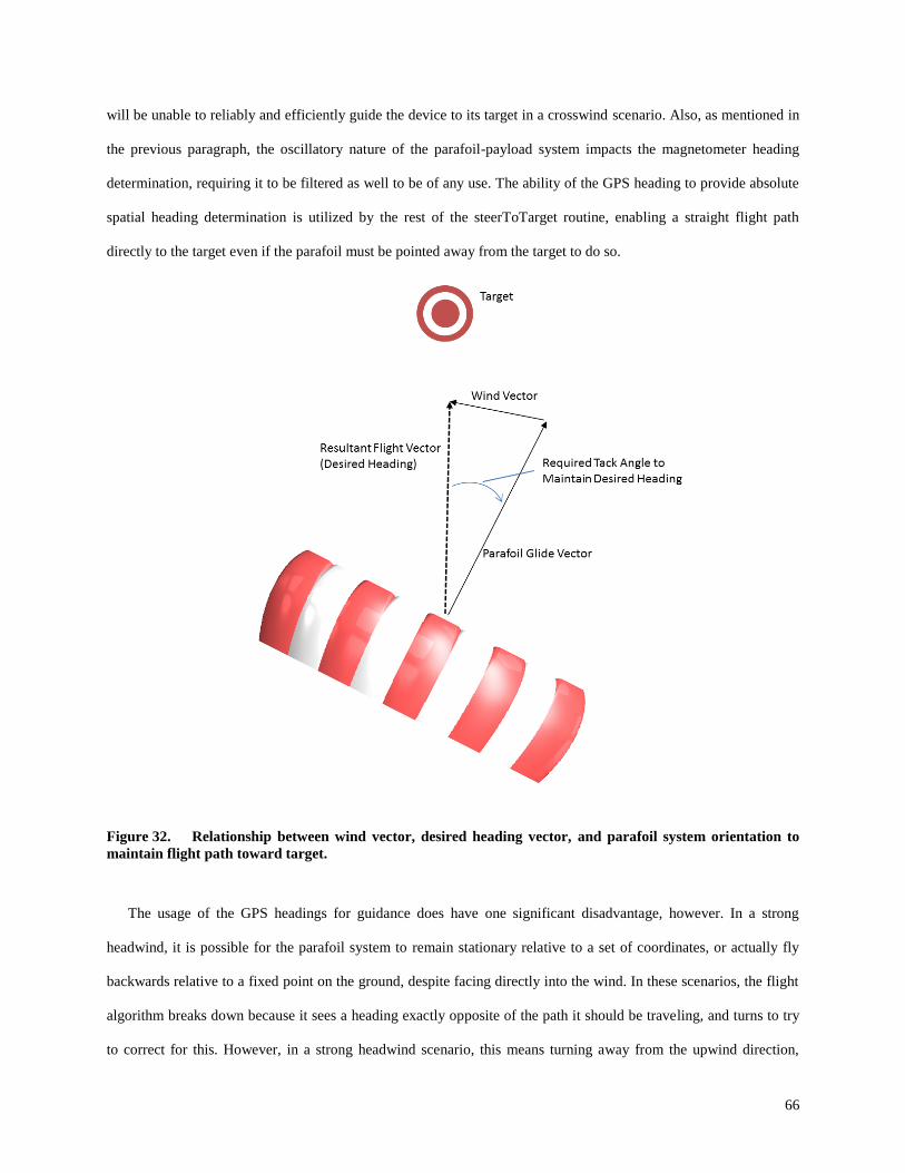
66
will be unable to reliably and efficiently guide the device to its target in a crosswind scenario. Also, as mentioned in
the previous paragraph, the oscillatory nature of the parafoil-payload system impacts the magnetometer heading
determination, requiring it to be filtered as well to be of any use. The ability of the GPS heading to provide absolute
spatial heading determination is utilized by the rest of the steerToTarget routine, enabling a straight flight path
directly to the target even if the parafoil must be pointed away from the target to do so.
Figure 32. Relationship between wind vector, desired heading vector, and parafoil system orientation to
maintain flight path toward target.
The usage of the GPS headings for guidance does have one significant disadvantage, however. In a strong
headwind, it is possible for the parafoil system to remain stationary relative to a set of coordinates, or actually fly
backwards relative to a fixed point on the ground, despite facing directly into the wind. In these scenarios, the flight
algorithm breaks down because it sees a heading exactly opposite of the path it should be traveling, and turns to try
to correct for this. However, in a strong headwind scenario, this means turning away from the upwind direction,
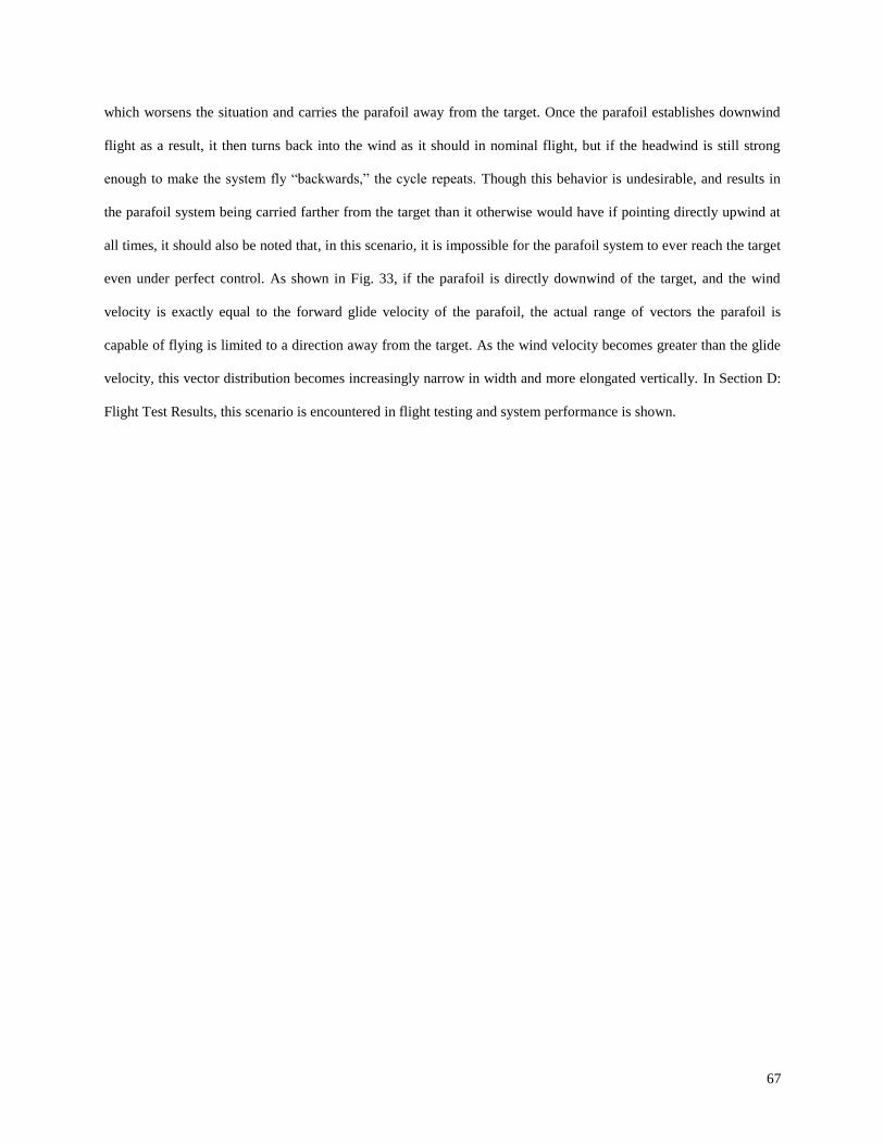
67
which worsens the situation and carries the parafoil away from the target. Once the parafoil establishes downwind
flight as a result, it then turns back into the wind as it should in nominal flight, but if the headwind is still strong
enough to make the system fly “backwards,” the cycle repeats. Though this behavior is undesirable, and results in
the parafoil system being carried farther from the target than it otherwise would have if pointing directly upwind at
all times, it should also be noted that, in this scenario, it is impossible for the parafoil system to ever reach the target
even under perfect control. As shown in Fig. 33, if the parafoil is directly downwind of the target, and the wind
velocity is exactly equal to the forward glide velocity of the parafoil, the actual range of vectors the parafoil is
capable of flying is limited to a direction away from the target. As the wind velocity becomes greater than the glide
velocity, this vector distribution becomes increasingly narrow in width and more elongated vertically. In Section D:
Flight Test Results, this scenario is encountered in flight testing and system performance is shown.
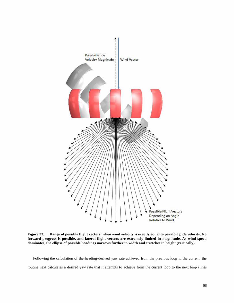
68
Figure 33. Range of possible flight vectors, when wind velocity is exactly equal to parafoil glide velocity. No
forward progress is possible, and lateral flight vectors are extremely limited in magnitude. As wind speed
dominates, the ellipse of possible headings narrows further in width and stretches in height (vertically).
Following the calculation of the heading-derived yaw rate achieved from the previous loop to the current, the
routine next calculates a desired yaw rate that it attempts to achieve from the current loop to the next loop (lines
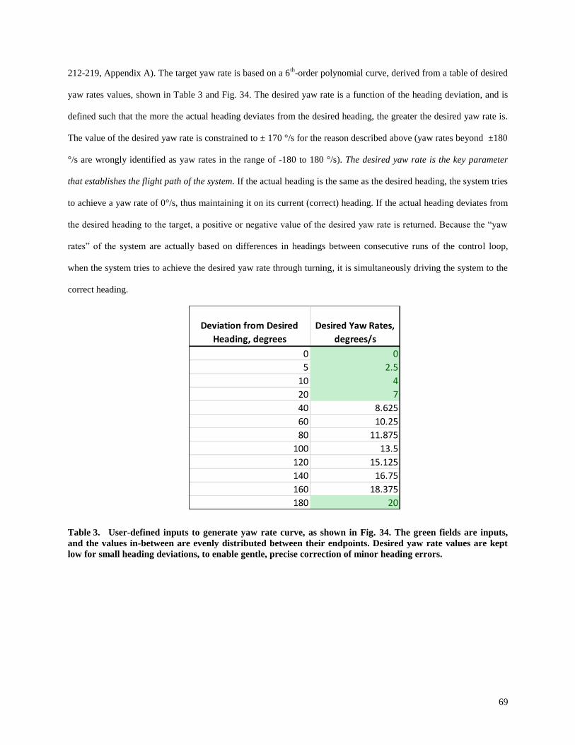
69
212-219, Appendix A). The target yaw rate is based on a 6th
-order polynomial curve, derived from a table of desired
yaw rates values, shown in Table 3 and Fig. 34. The desired yaw rate is a function of the heading deviation, and is
defined such that the more the actual heading deviates from the desired heading, the greater the desired yaw rate is.
The value of the desired yaw rate is constrained to ± 170 °/s for the reason described above (yaw rates beyond ±180
°/s are wrongly identified as yaw rates in the range of -180 to 180 °/s). The desired yaw rate is the key parameter
that establishes the flight path of the system. If the actual heading is the same as the desired heading, the system tries
to achieve a yaw rate of 0°/s, thus maintaining it on its current (correct) heading. If the actual heading deviates from
the desired heading to the target, a positive or negative value of the desired yaw rate is returned. Because the “yaw
rates” of the system are actually based on differences in headings between consecutive runs of the control loop,
when the system tries to achieve the desired yaw rate through turning, it is simultaneously driving the system to the
correct heading.
Table 3. User-defined inputs to generate yaw rate curve, as shown in Fig. 34. The green fields are inputs,
and the values in-between are evenly distributed between their endpoints. Desired yaw rate values are kept
low for small heading deviations, to enable gentle, precise correction of minor heading errors.
Deviation from Desired
Heading, degrees
Desired Yaw Rates,
degrees/s
0 0
5 2.5
10 4
20 7
40 8.625
60 10.25
80 11.875
100 13.5
120 15.125
140 16.75
160 18.375
180 20
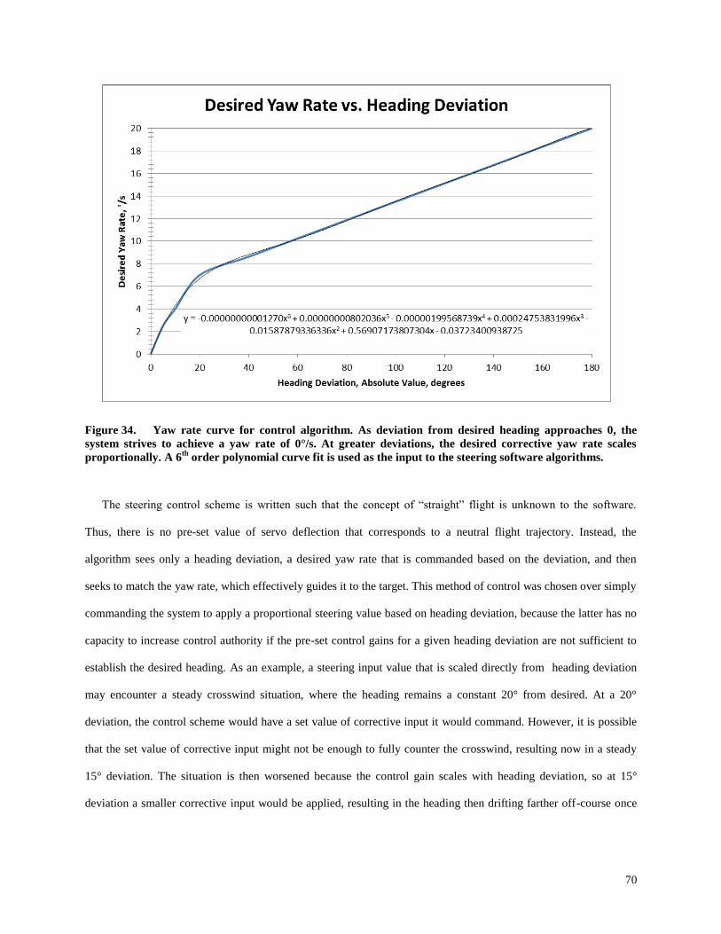
70
Figure 34. Yaw rate curve for control algorithm. As deviation from desired heading approaches 0, the
system strives to achieve a yaw rate of 0°/s. At greater deviations, the desired corrective yaw rate scales
proportionally. A 6th
order polynomial curve fit is used as the input to the steering software algorithms.
The steering control scheme is written such that the concept of “straight” flight is unknown to the software.
Thus, there is no pre-set value of servo deflection that corresponds to a neutral flight trajectory. Instead, the
algorithm sees only a heading deviation, a desired yaw rate that is commanded based on the deviation, and then
seeks to match the yaw rate, which effectively guides it to the target. This method of control was chosen over simply
commanding the system to apply a proportional steering value based on heading deviation, because the latter has no
capacity to increase control authority if the pre-set control gains for a given heading deviation are not sufficient to
establish the desired heading. As an example, a steering input value that is scaled directly from heading deviation
may encounter a steady crosswind situation, where the heading remains a constant 20° from desired. At a 20°
deviation, the control scheme would have a set value of corrective input it would command. However, it is possible
that the set value of corrective input might not be enough to fully counter the crosswind, resulting now in a steady
15° deviation. The situation is then worsened because the control gain scales with heading deviation, so at 15°
deviation a smaller corrective input would be applied, resulting in the heading then drifting farther off-course once
71
more. Though a steering scheme of this type is highly effective in a perfectly windless scenario, it’s easy to see its
shortcomings in real-life applications.
To solve the problem just described, the control routine of this work looks at the actual heading difference
achieved between consecutive loops—this is the “achieved yaw rate” described above. If it is found that the system
did not achieve the desired yaw rate during the previous loop, it scales up the next steering command by a fixed
percentage (at two different thresholds of precision, depending on the magnitude of deviation), and then looks at the
effect of this new steering command in the next loop. If the target yaw rate is still not achieved, it continues
increasing the steering command each loop until it is matched. If the target yaw rate is overshot, then the steering
command is scaled back. If the target yaw rate is within a defined deadband threshold of the achieved yaw rate (this
is the parameter DESIRED_YAW_DEADBAND), it maintains the same servo commands for the next loop. If the
control system is sufficiently close to the correct heading (where “sufficient” is determined by another deadband
parameter, HEADING_DEADBAND), it also maintains the same servo commands for the next loop, and adjusts
them again only after either the heading veers beyond the heading deadband or the achieved yaw rate strays beyond
the yaw rate deadband. Though a bit confusing in description, this method of control compensates for any trim
errors (meaning that if the parafoil has a tendency to veer slightly left or right with no steering input, it is of no
consequence to the control system), and will drive the system to the correct heading even if that means pointing at a
sharp angle into the wind.
The actual process of the control scaling routine can be found in lines 238-278 of Appendix A. Specifically, it
operates as follows:
(1) If the desired turn direction (right/left) changed in the previous loop due to crossing over the desired
heading, or the system is within the desired heading deadband and is maintaining the servo deflections at
constant values, the servo pull values are reset to zero. In the case of flying within the heading deadband,
the servos will not be updated to the reset position until the device heading exits the deadband range.
(2) If the steerDelayCounter is active (meaning a value of NUM_LOOPS_BEFORE_SCALING_TURN >
1), the steering gain calculation does not occur until the specified number of loops. This is an easy means
to “numb” the control response in case the system is found to be over-controlling. (In testing, it was
found that this parameter is not necessary, as varying the servo scaling step percentages achieves the
same result and provides smoother control from the servos because they update at a higher frequency.)
72
(3) If the yaw rate error from desired to achieved is greater than the yaw rate deadband, and the system is
not flying within the heading deviation deadband, steering scaling occurs for the loop. Otherwise the
values are left unchanged until the next loop.
(4) If the achieved yaw rate and desired yaw rate are different in sign (e.g. +/-), and the yaw rate error from
actual to desired is less than FINE_SCALING_CUTOFF_DEG_SEC, the servo command for this loop is
increased by the value FINE_SCALING_STEP_PERCENT.
(5) If the achieved yaw rate and desired yaw rate are different in sign, and the yaw rate error is greater than
FINE_SCALING_CUTOFF_DEG_SEC, the servo command for this loop is increased by the value
COARSE_SCALING_STEP_PERCENT.
(6) If the desired and achieved yaw rates are of the same sign, and the yaw rate error is less than
FINE_SCALING_CUTOFF_DEG_SEC, and the actual yaw rate magnitude is less than the desired
magnitude, the servo command for this loop is increased by the value
FINE_SCALING_STEP_PERCENT.
(7) If the desired and achieved yaw rates are of the same sign, and the yaw rate error is less than
FINE_SCALING_CUTOFF_DEG_SEC, and the actual yaw rate magnitude is greater than the desired
magnitude, the servo command for this loop is decreased by the value
FINE_SCALING_STEP_PERCENT.
(8) If the desired and achieved yaw rates are of the same sign, and the yaw rate error is greater than
FINE_SCALING_CUTOFF_DEG_SEC, and the actual yaw rate magnitude is less than the desired
magnitude, the servo command for this loop is increased by the value
COARSE_SCALING_STEP_PERCENT.
(9) If the desired and achieved yaw rates are of the same sign, and the yaw rate error is greater than
FINE_SCALING_CUTOFF_DEG_SEC, and the actual yaw rate magnitude is greater than the desired
magnitude, the servo command for this loop is decreased by the value
COARSE_SCALING_STEP_PERCENT.
After determining the change to be made to the servo pull value for the current loop as outlined above, the
value is stored in the array variable steeringScale[0]. Prior to storing the value, the steeringScale value of the
73
previous loop is written to steeringScale[1], to enable the carrying of current and previous values for control
routine validation and/or debugging.
Next, the steeringScale value is limited to a maximum of 1 or -1, which both represent 100% servo
deflection. This prevents the system from commanding a servo response beyond the operational range of the
servo control system. The final steering command value is then written to another array variable,
servoOutPrcnt[0].
Prior to this point, no determination has been made in regards to which direction to steer—instead, only the
value to command the steering servo has been calculated. The next lines of the code (lines 304-348, Appendix
A) make the determination in regards to which direction to steer, and then initiate the command that actually
moves one or both of the servos. The logic of this routine is as follows:
(1) If the heading deviation, headingDev, is less than –HEADING_DEADBAND, and the commanded
servo value, servoOutPrcnt[0] is greater than or equal to 0; or, if headingDev is greater than
+HEADING_DEADBAND and servoOutPrcnt[0] is less than zero, turn LEFT. The left servo is sent a
command to move to the value of servoOutPrcnt[0] and the right servo is set to neutral. Also, if the left
turn occurred as a result of a positive servoOutPrcnt value, a flag is set for the variable turnedLeft. (This
flag is used for a complex nuance of the steering scaling routine, because negative steering percent
values only occur if the system has been steering toward a desired yaw rate, overshot the value, and is
trying to reduce it, but the flight path still has not crossed over to the other side of the desired heading.
The actual purpose of the flag is to prevent a control logic error that occurs as a result of the above.)
(2) If the heading deviation, headingDev, is greater than HEADING_DEADBAND, and the commanded
servo value, servoOutPrcnt[0] is greater than or equal to 0; or, if headingDev is less than -
HEADING_DEADBAND and servoOutPrcnt[0] is less than zero, turn RIGHT. The right servo is sent a
command to move to the value of servoOutPrcnt[0] and the left servo is set to neutral. Also, if the right
turn occurred as a result of a positive servoOutPrcnt value, a flag is set for the variable turnedRight. (See
the note above regarding the function of this flag variable.)
(3) If none of the above conditions are met, the turnedLeft and turnedRight flags are reset, and the servos are
left unchanged from the previous loop. In this scenario, the system logically must be within the heading
deadband, and is thus flying toward the target.
74
At this point, the steering scaling routine is nearly complete. If steering occurred during this loop, a flag is set
for the array variable steeringActive[0], which is used to disable the reset of the steering scale value during the next
loop, so that further servo corrections are added or subtracted to the current servo position. The final phase of the
routine is to write back all array variables (with a couple of exceptions, which are written earlier for logic reasons)
from the [0] position to the [1] position, so that they may be used in the control logic of the next loop. At this point,
the routine exits, and returns to the main control loop, simple_control().
The steerToTarget routine is complex, but in summary, it does the following:
Determines deviations from the desired heading and desired yaw rate when updates are available from
the GPS.
Adds or subtracts either a fine or coarse step value to one of the servos to try to achieve the desired yaw
rate.
Sends the steering command to the servos and repeats, at a rate of ten times per second, unless the
control loop initiates the landing routine or landing flare.
4. Landing Routine – “landingRoutine()”
(User-defined input constants used in this function: LANDING_RADIUS_THRESHOLD, HEADING_DEADBAND,
NUM_LOOPS_BEFORE_SCALING_TURN_LANDING, DESIRED_YAW_DEADBAND, LANDING_RADIUS,
DEGREES_TO_RAD, SERVO_RIGHT_WINCH_3, SERVO_LEFT_WINCH_4, SERVO_R_WINCH_MAX_TRAVEL,
SERVO_L_WINCH_MAX_TRAVEL, SERVO_R_WINCH_SCALE_FACTOR,
SERVO_L_WINCH_SCALE_FACTOR, FINE_SCALING_UNWIND_GAIN, COARSE_SCALING_UNWIND_GAIN)
The landing routine is very similar in operation to the steerToTarget routine, so each individual step will
not be described in detail. Instead, the differences between the two will be noted.
The landing routine is essentially the same routine as steerToTarget, with two key differences: the desired
heading is actually a heading 90° from the heading to the target, which results in a circular flight path around
the target, and the desired yaw rate is calculated from the size of the desired landing circle size, defined by
the constant LANDING_RADIUS.
Before determining the actual heading to fly, the routine first determines whether the parafoil system is
approaching the target from the left, or from the right. In the former case, it is then desirable to fly a spiral to
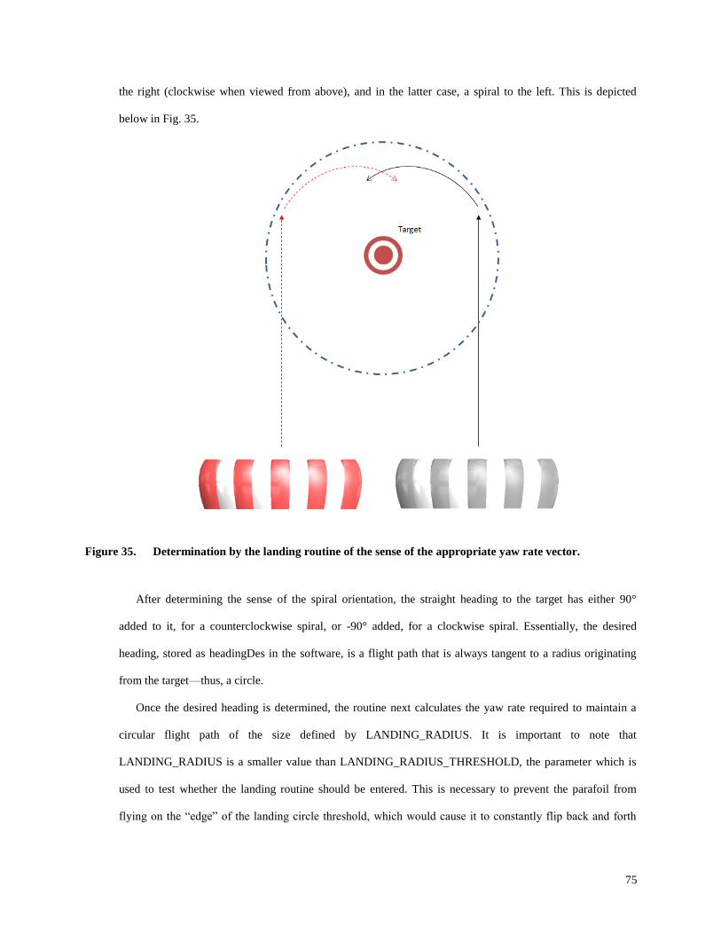
75
the right (clockwise when viewed from above), and in the latter case, a spiral to the left. This is depicted
below in Fig. 35.
Figure 35. Determination by the landing routine of the sense of the appropriate yaw rate vector.
After determining the sense of the spiral orientation, the straight heading to the target has either 90°
added to it, for a counterclockwise spiral, or -90° added, for a clockwise spiral. Essentially, the desired
heading, stored as headingDes in the software, is a flight path that is always tangent to a radius originating
from the target—thus, a circle.
Once the desired heading is determined, the routine next calculates the yaw rate required to maintain a
circular flight path of the size defined by LANDING_RADIUS. It is important to note that
LANDING_RADIUS is a smaller value than LANDING_RADIUS_THRESHOLD, the parameter which is
used to test whether the landing routine should be entered. This is necessary to prevent the parafoil from
flying on the “edge” of the landing circle threshold, which would cause it to constantly flip back and forth
76
between the landingRoutine and steerToTarget routines. The yaw rate required, desiredYawRate[0], is
calculated from the following simple line of code:
desiredYawRate[0]= (headingDev/fabs(headingDev) * g.GPSgndspeed / LANDING_RADIUS) *
RAD_TO_DEG;
(6)
This line of code is the same as the familiar expression relating tangential velocity to angular velocity for
rigid body motion about a fixed axis:
(7)
In the case of the software code, the tangential velocity vt is the same as g.GPSgndspeed, which is the
magnitude of the horizontal flight velocity in the direction of the flight heading, provided by the on-board
GPS. The sense of the yaw rate, positive or negative, is determined by headingDev/fabs(headingDev), which
is the value of the heading deviation from actual to desired, divided by the absolute value of the same. Thus,
if the heading deviation is negative, the calculated desired yaw rate will also be negative (resulting in a left
turn towards the correct heading), and vice versa. Unlike the steerToTarget determination of desired yaw
rate, the value here is not scaled based on deviation from the desired heading. Instead, the value is dependent
on the parafoil turning at a constant rate at the given tangential velocity, which will produce a circular flight
path of the desired radius if the actual yaw rate is maintained reasonably close to the desired value.
At this point, the remainder of the landingRoutine process is nearly identical to the steerToTarget routine.
There are a couple of very important limitations to the landingRoutine process, however. First, the selection
of the LANDING_RADIUS and LANDING_RADIUS_THRESHOLD values is not trivial. If
LANDING_RADIUS is too small, the yaw rate required to maintain a circular pattern of that size may
exceed the ±180°/s limitation imposed by the achievedYawRate calculation logic, as discussed previously.
The software contains a line to prevent this scenario that limits the maximum commanded yaw rate to
±170°/s, but if this condition must be imposed, the desired landing circle size obviously will not be achieved.
Second, and even more crucial, LANDING_RADIUS must be large enough to ensure that the parafoil does
not fly through the landing circle and out the other side before it has time to begin circling. Even at maximum
control deflections, the parafoil is not extremely quick to respond to control inputs, and flight testing has
shown that to “wind up” to a yaw rate of 30°/s or so (typical for tested values of the landing spiral size)
77
requires at least a few seconds. At an average forward velocity of 5.5 m/s (depending on payload mass), it
requires only a couple of seconds to fly completely through a landing circle of 10 m diameter. In the
helicopter flight tests discussed in Section D: Flight Test Results, this is exactly what occurred, and upon
exiting the landing circle, the parafoil system returned to the steerToTarget routine, flew itself back into the
circle, and back out once more before running out of altitude.
A final limitation of the landing circle routine is wind velocity. If the prevailing winds are greater than the
normal forward glide velocity of the parafoil, the system will eventually be pushed out of the landing circle
in the direction of the wind vector, and will not be able to fly back upwind to the target. This is a
consequence of not having any form of propulsion, and cannot be mitigated unless the flight is initiated
upwind of the target, and new control logic is implemented to make the parafoil descend more rapidly to the
target before it crosses it. This functionality is not present in the current software but will be added at a later
date to improve its robustness. Indeed, in one of the UAV drop tests described in Section D: Flight Test
Results, this very behavior was observed when the parafoil approached the target from upwind, flew exactly
to the target coordinate, achieved two spiral turns, and then was blown past the target in very high winds.
Despite navigating precisely to the target initially, it ultimately landed approximately 100 m downwind.
5. Landing Flare Routine – “landingFlare()”
(User-defined input constants used in this function: SERVO_RIGHT_WINCH_3, SERVO_LEFT_WINCH_4,
SERVO_R_WINCH_MAX_TRAVEL, SERVO_L_WINCH_MAX_TRAVEL, SERVO_R_WINCH_SCALE_FACTOR,
SERVO_L_WINCH_SCALE_FACTOR, FLARE_PRCNT)
The landing flare routine, landingFlare(), is a very simple function which attempts to slow the rate of descent of
the parafoil just prior to touchdown. It relies on knowledge of the altitude of target coordinate, and initiates a flare
maneuver when the parafoil system is FLARE_HEIGHT m above the target altitude, as determined by GPS. When
this condition occurs, it simply sets both servos to an equal pull value of FLARE_PRCNT, which increases the
camber, lift, and drag of the parafoil, and causes it to descend more slowly. This also serves to terminate the spiral of
the landing routine just prior to touchdown.
This routine is still experimental at the time of writing, and was only successfully demonstrated in one low-
altitude test. A number of limitations exist in its use. First, the GPS altitude value is one of the least precise
parameters reported by the GPS, and even with a very strong link tracking many satellites, it routinely fluctuates by
78
10 m or more. Altitude precision is made even worse by a moving and descending system, while the precision
improves if the device is left stationary on the ground. For this reason, it is necessary to specify the initiation of the
landing flare maneuver at a higher than desirable altitude to ensure that it is initiated at all prior to touchdown.
A second limitation, which could be corrected rather easily in the software code, is that the system will enter the
landing routine at a given altitude (referenced to sea level) regardless of its proximity to the landing target. As an
unlikely example, if the parafoil system is flying over a deep ravine, with the ground elevation much lower than that
of the target, the parafoil will still enter the flare routine near the target altitude, stall, and descend uncontrolled to
the ground. A simple conditional statement to only enter the landing flare routine when within a given proximity of
the target will remedy this issue easily, and will be implemented in a future version of the software.
D. Flight Test Results
1. Testing Methods
To verify the performance of the many iterations of the steering routine written for this work, three levels of
testing were used. For initial code performance assessment, and to eliminate any obvious functionality bugs, the
software was first compiled to run on a Windows-based computer, and a large set of fictitious flight data was
supplied to the flight algorithm. For each run of the control loop, the software was set up to write all of the
critical control parameters to the screen. Sample output from one of these data simulation runs is shown in Fig.
36. Compiling the software and testing it in this fashion takes less than a minute, so this method was used
regularly throughout the software writing process to ensure obvious logic errors were caught prior to flight
testing.
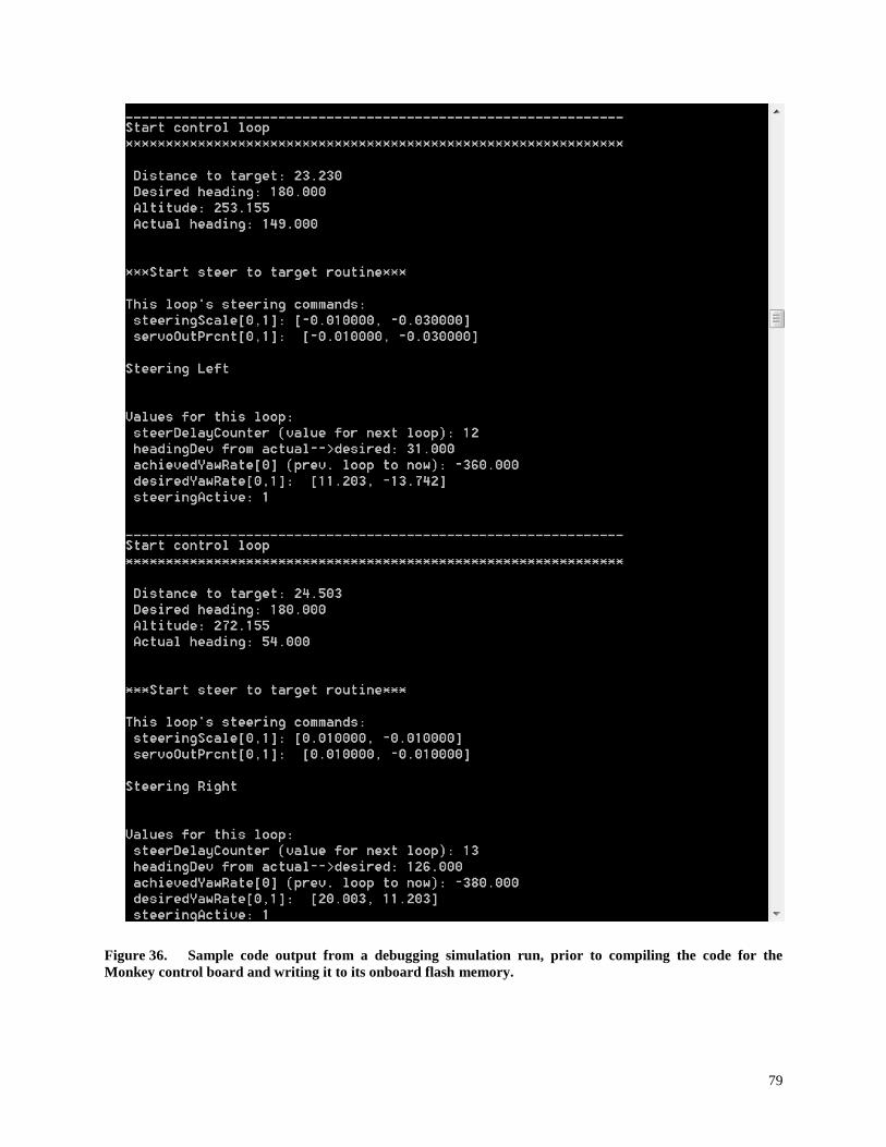
79
Figure 36. Sample code output from a debugging simulation run, prior to compiling the code for the
Monkey control board and writing it to its onboard flash memory.
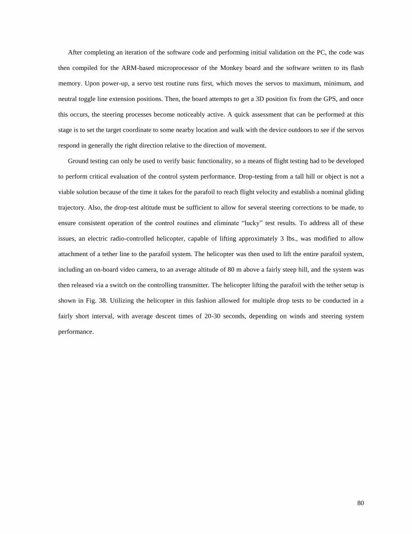
80
After completing an iteration of the software code and performing initial validation on the PC, the code was
then compiled for the ARM-based microprocessor of the Monkey board and the software written to its flash
memory. Upon power-up, a servo test routine runs first, which moves the servos to maximum, minimum, and
neutral toggle line extension positions. Then, the board attempts to get a 3D position fix from the GPS, and once
this occurs, the steering processes become noticeably active. A quick assessment that can be performed at this
stage is to set the target coordinate to some nearby location and walk with the device outdoors to see if the servos
respond in generally the right direction relative to the direction of movement.
Ground testing can only be used to verify basic functionality, so a means of flight testing had to be developed
to perform critical evaluation of the control system performance. Drop-testing from a tall hill or object is not a
viable solution because of the time it takes for the parafoil to reach flight velocity and establish a nominal gliding
trajectory. Also, the drop-test altitude must be sufficient to allow for several steering corrections to be made, to
ensure consistent operation of the control routines and eliminate “lucky” test results. To address all of these
issues, an electric radio-controlled helicopter, capable of lifting approximately 3 lbs., was modified to allow
attachment of a tether line to the parafoil system. The helicopter was then used to lift the entire parafoil system,
including an on-board video camera, to an average altitude of 80 m above a fairly steep hill, and the system was
then released via a switch on the controlling transmitter. The helicopter lifting the parafoil with the tether setup is
shown in Fig. 38. Utilizing the helicopter in this fashion allowed for multiple drop tests to be conducted in a
fairly short interval, with average descent times of 20-30 seconds, depending on winds and steering system
performance.
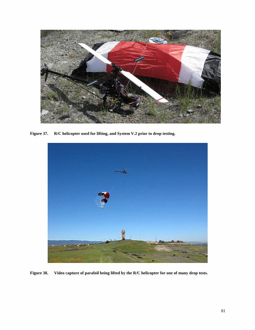
81
Figure 37. R/C helicopter used for lifting, and System V.2 prior to drop testing.
Figure 38. Video capture of parafoil being lifted by the R/C helicopter for one of many drop tests.
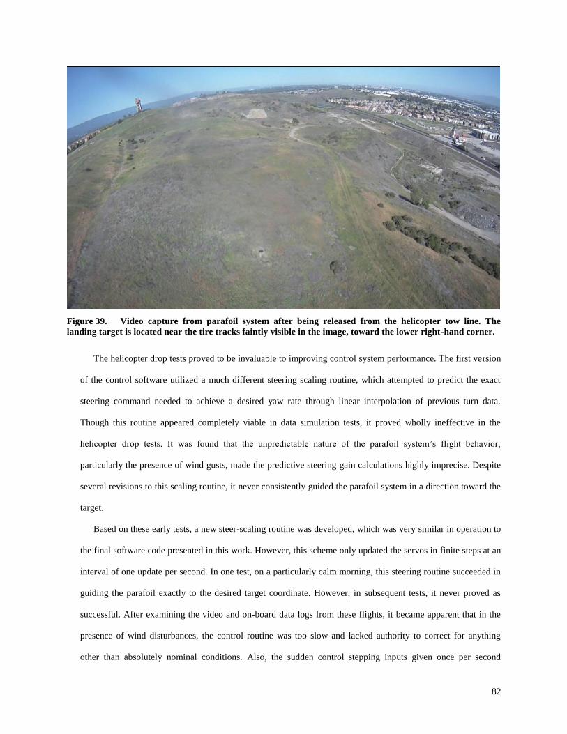
82
Figure 39. Video capture from parafoil system after being released from the helicopter tow line. The
landing target is located near the tire tracks faintly visible in the image, toward the lower right-hand corner.
The helicopter drop tests proved to be invaluable to improving control system performance. The first version
of the control software utilized a much different steering scaling routine, which attempted to predict the exact
steering command needed to achieve a desired yaw rate through linear interpolation of previous turn data.
Though this routine appeared completely viable in data simulation tests, it proved wholly ineffective in the
helicopter drop tests. It was found that the unpredictable nature of the parafoil system’s flight behavior,
particularly the presence of wind gusts, made the predictive steering gain calculations highly imprecise. Despite
several revisions to this scaling routine, it never consistently guided the parafoil system in a direction toward the
target.
Based on these early tests, a new steer-scaling routine was developed, which was very similar in operation to
the final software code presented in this work. However, this scheme only updated the servos in finite steps at an
interval of one update per second. In one test, on a particularly calm morning, this steering routine succeeded in
guiding the parafoil exactly to the desired target coordinate. However, in subsequent tests, it never proved as
successful. After examining the video and on-board data logs from these flights, it became apparent that in the
presence of wind disturbances, the control routine was too slow and lacked authority to correct for anything
other than absolutely nominal conditions. Also, the sudden control stepping inputs given once per second
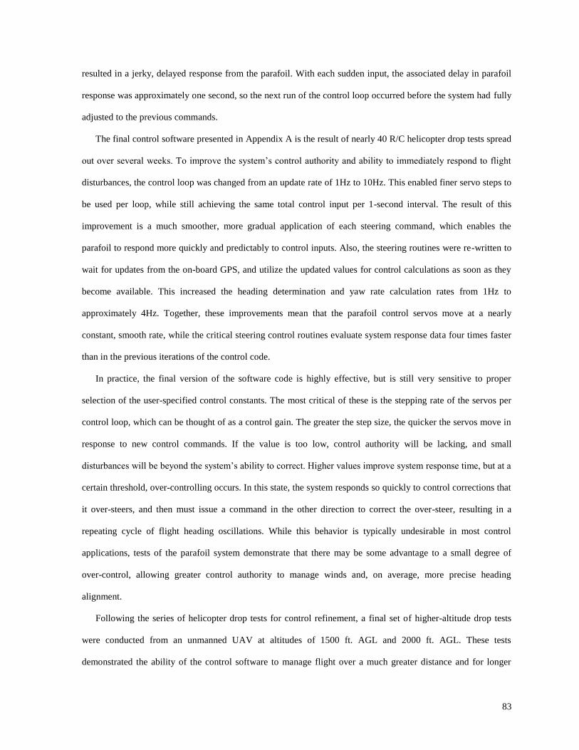
83
resulted in a jerky, delayed response from the parafoil. With each sudden input, the associated delay in parafoil
response was approximately one second, so the next run of the control loop occurred before the system had fully
adjusted to the previous commands.
The final control software presented in Appendix A is the result of nearly 40 R/C helicopter drop tests spread
out over several weeks. To improve the system’s control authority and ability to immediately respond to flight
disturbances, the control loop was changed from an update rate of 1Hz to 10Hz. This enabled finer servo steps to
be used per loop, while still achieving the same total control input per 1-second interval. The result of this
improvement is a much smoother, more gradual application of each steering command, which enables the
parafoil to respond more quickly and predictably to control inputs. Also, the steering routines were re-written to
wait for updates from the on-board GPS, and utilize the updated values for control calculations as soon as they
become available. This increased the heading determination and yaw rate calculation rates from 1Hz to
approximately 4Hz. Together, these improvements mean that the parafoil control servos move at a nearly
constant, smooth rate, while the critical steering control routines evaluate system response data four times faster
than in the previous iterations of the control code.
In practice, the final version of the software code is highly effective, but is still very sensitive to proper
selection of the user-specified control constants. The most critical of these is the stepping rate of the servos per
control loop, which can be thought of as a control gain. The greater the step size, the quicker the servos move in
response to new control commands. If the value is too low, control authority will be lacking, and small
disturbances will be beyond the system’s ability to correct. Higher values improve system response time, but at a
certain threshold, over-controlling occurs. In this state, the system responds so quickly to control corrections that
it over-steers, and then must issue a command in the other direction to correct the over-steer, resulting in a
repeating cycle of flight heading oscillations. While this behavior is typically undesirable in most control
applications, tests of the parafoil system demonstrate that there may be some advantage to a small degree of
over-control, allowing greater control authority to manage winds and, on average, more precise heading
alignment.
Following the series of helicopter drop tests for control refinement, a final set of higher-altitude drop tests
were conducted from an unmanned UAV at altitudes of 1500 ft. AGL and 2000 ft. AGL. These tests
demonstrated the ability of the control software to manage flight over a much greater distance and for longer
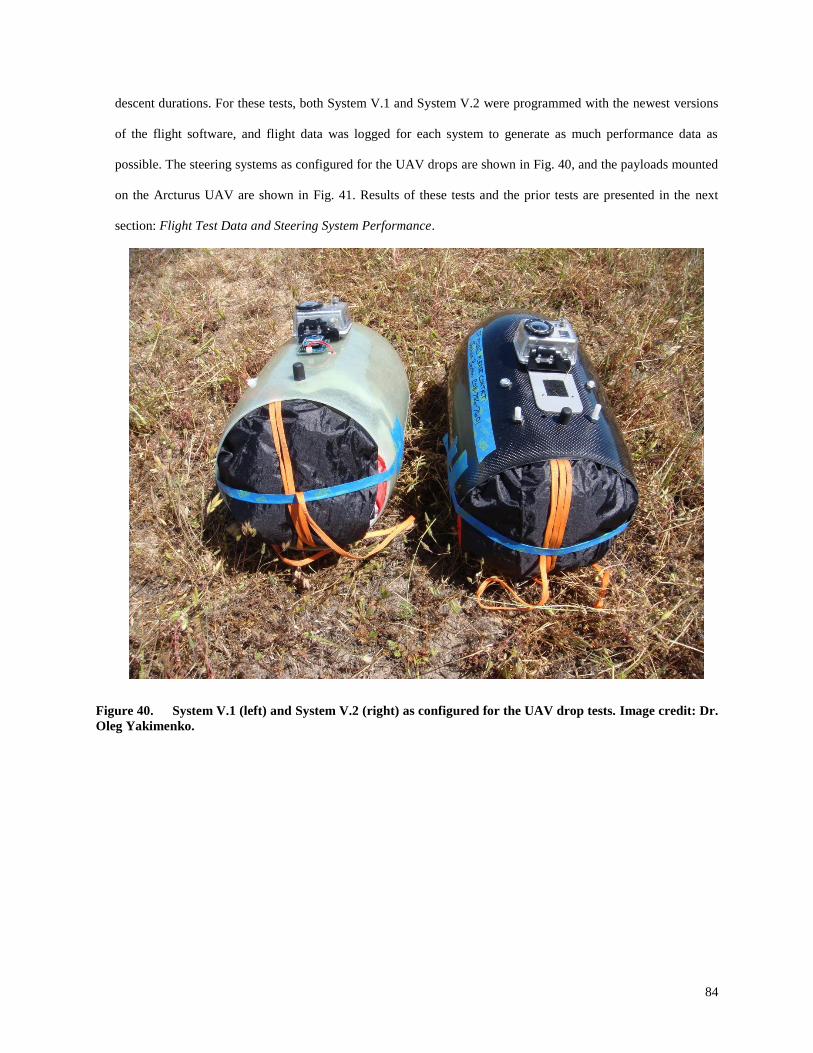
84
descent durations. For these tests, both System V.1 and System V.2 were programmed with the newest versions
of the flight software, and flight data was logged for each system to generate as much performance data as
possible. The steering systems as configured for the UAV drops are shown in Fig. 40, and the payloads mounted
on the Arcturus UAV are shown in Fig. 41. Results of these tests and the prior tests are presented in the next
section: Flight Test Data and Steering System Performance.
Figure 40. System V.1 (left) and System V.2 (right) as configured for the UAV drop tests. Image credit: Dr.
Oleg Yakimenko.
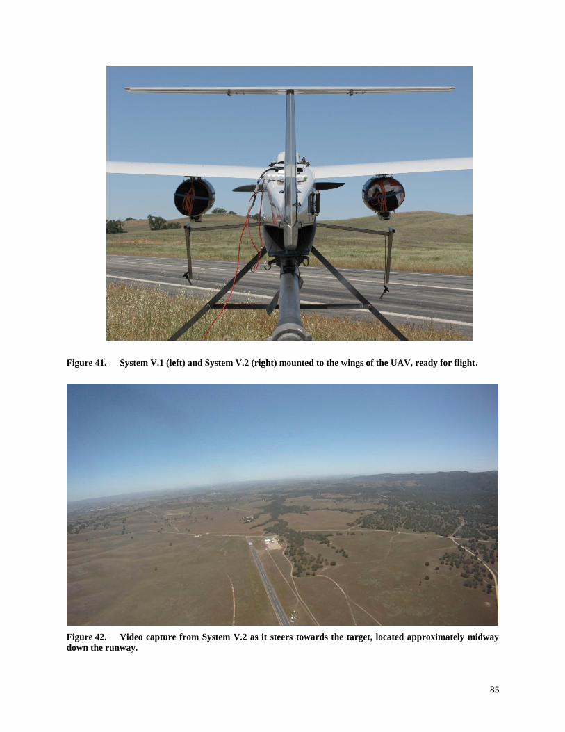
85
Figure 41. System V.1 (left) and System V.2 (right) mounted to the wings of the UAV, ready for flight.
Figure 42. Video capture from System V.2 as it steers towards the target, located approximately midway
down the runway.
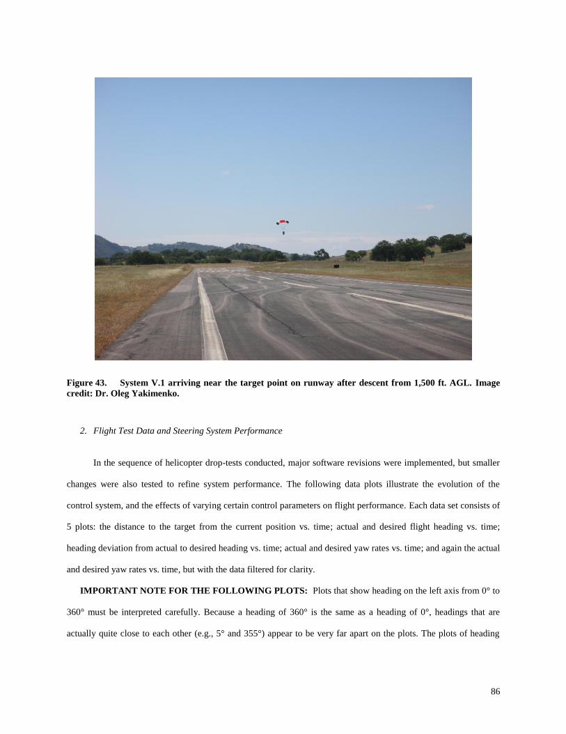
86
Figure 43. System V.1 arriving near the target point on runway after descent from 1,500 ft. AGL. Image
credit: Dr. Oleg Yakimenko.
2. Flight Test Data and Steering System Performance
In the sequence of helicopter drop-tests conducted, major software revisions were implemented, but smaller
changes were also tested to refine system performance. The following data plots illustrate the evolution of the
control system, and the effects of varying certain control parameters on flight performance. Each data set consists of
5 plots: the distance to the target from the current position vs. time; actual and desired flight heading vs. time;
heading deviation from actual to desired heading vs. time; actual and desired yaw rates vs. time; and again the actual
and desired yaw rates vs. time, but with the data filtered for clarity.
IMPORTANT NOTE FOR THE FOLLOWING PLOTS: Plots that show heading on the left axis from 0° to
360° must be interpreted carefully. Because a heading of 360° is the same as a heading of 0°, headings that are
actually quite close to each other (e.g., 5° and 355°) appear to be very far apart on the plots. The plots of heading
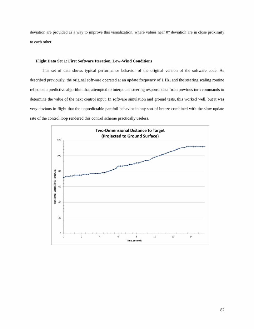
87
deviation are provided as a way to improve this visualization, where values near 0° deviation are in close proximity
to each other.
Flight Data Set 1: First Software Iteration, Low-Wind Conditions
This set of data shows typical performance behavior of the original version of the software code. As
described previously, the original software operated at an update frequency of 1 Hz, and the steering scaling routine
relied on a predictive algorithm that attempted to interpolate steering response data from previous turn commands to
determine the value of the next control input. In software simulation and ground tests, this worked well, but it was
very obvious in flight that the unpredictable parafoil behavior in any sort of breeze combined with the slow update
rate of the control loop rendered this control scheme practically useless.
0
20
40
60
80
100
120
0 2 4 6 8 10 12 14
Ho
rizo
nta
l Dis
tan
ce t
o T
arge
t, m
Time, seconds
Two-Dimensional Distance to Target(Projected to Ground Surface)
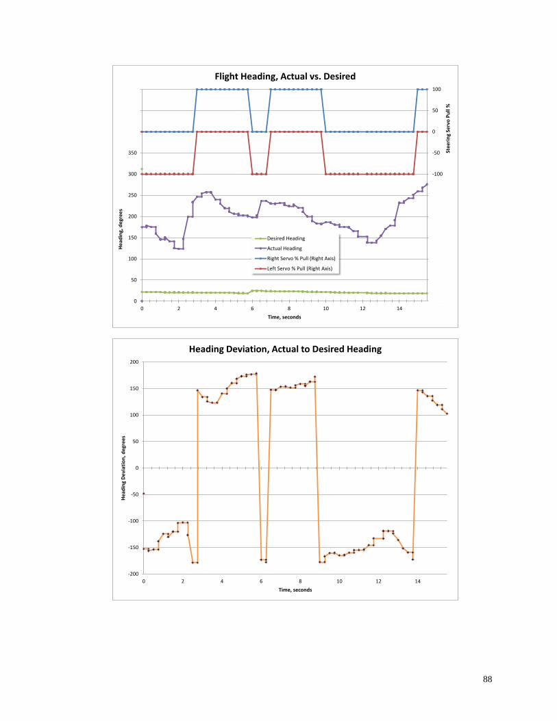
88
-400
-350
-300
-250
-200
-150
-100
-50
0
50
100
0
50
100
150
200
250
300
350
400
450
500
0 2 4 6 8 10 12 14
Ste
eri
ng
Serv
o P
ull
%
He
adin
g, d
egr
ee
s
Time, seconds
Flight Heading, Actual vs. Desired
Desired Heading
Actual Heading
Right Servo % Pull (Right Axis)
Left Servo % Pull (Right Axis)
-200
-150
-100
-50
0
50
100
150
200
0 2 4 6 8 10 12 14
He
adin
g D
evi
atio
n,
de
gre
es
Time, seconds
Heading Deviation, Actual to Desired Heading
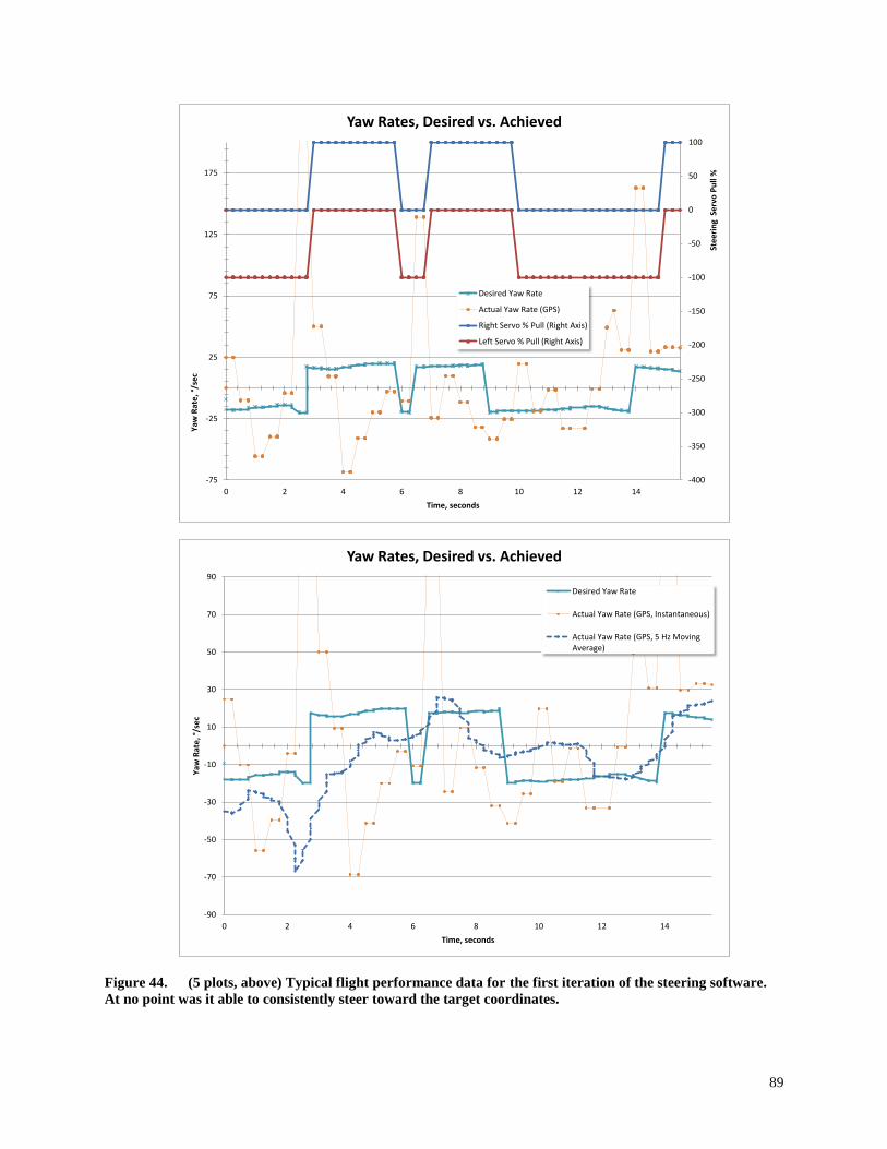
89
Figure 44. (5 plots, above) Typical flight performance data for the first iteration of the steering software.
At no point was it able to consistently steer toward the target coordinates.
-400
-350
-300
-250
-200
-150
-100
-50
0
50
100
-75
-25
25
75
125
175
0 2 4 6 8 10 12 14
Ste
eri
ng
Se
rvo
Pu
ll %
Yaw
Rat
e, °
/se
c
Time, seconds
Yaw Rates, Desired vs. Achieved
Desired Yaw Rate
Actual Yaw Rate (GPS)
Right Servo % Pull (Right Axis)
Left Servo % Pull (Right Axis)
-90
-70
-50
-30
-10
10
30
50
70
90
0 2 4 6 8 10 12 14
Yaw
Rat
e, °
/se
c
Time, seconds
Yaw Rates, Desired vs. Achieved
Desired Yaw Rate
Actual Yaw Rate (GPS, Instantaneous)
Actual Yaw Rate (GPS, 5 Hz MovingAverage)
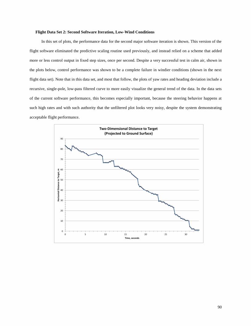
90
Flight Data Set 2: Second Software Iteration, Low-Wind Conditions
In this set of plots, the performance data for the second major software iteration is shown. This version of the
flight software eliminated the predictive scaling routine used previously, and instead relied on a scheme that added
more or less control output in fixed step sizes, once per second. Despite a very successful test in calm air, shown in
the plots below, control performance was shown to be a complete failure in windier conditions (shown in the next
flight data set). Note that in this data set, and most that follow, the plots of yaw rates and heading deviation include a
recursive, single-pole, low-pass filtered curve to more easily visualize the general trend of the data. In the data sets
of the current software performance, this becomes especially important, because the steering behavior happens at
such high rates and with such authority that the unfiltered plot looks very noisy, despite the system demonstrating
acceptable flight performance.
0
10
20
30
40
50
60
70
80
90
0 5 10 15 20 25 30
Ho
rizo
nta
l Dis
tan
ce t
o T
arge
t, m
Time, seconds
Two-Dimensional Distance to Target(Projected to Ground Surface)
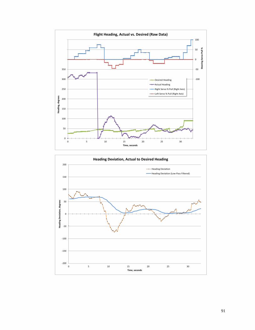
91
-400
-350
-300
-250
-200
-150
-100
-50
0
50
100
0
50
100
150
200
250
300
350
400
450
500
0 5 10 15 20 25 30
Ste
eri
ng
Serv
o P
ull
%
He
adin
g, d
egr
ee
s
Time, seconds
Flight Heading, Actual vs. Desired (Raw Data)
Desired Heading
Actual Heading
Right Servo % Pull (Right Axis)
Left Servo % Pull (Right Axis)
-200
-150
-100
-50
0
50
100
150
200
0 5 10 15 20 25 30
He
adin
g D
evi
atio
n,
de
gre
es
Time, seconds
Heading Deviation, Actual to Desired Heading
Heading Deviation
Heading Deviation (Low-Pass Filtered)
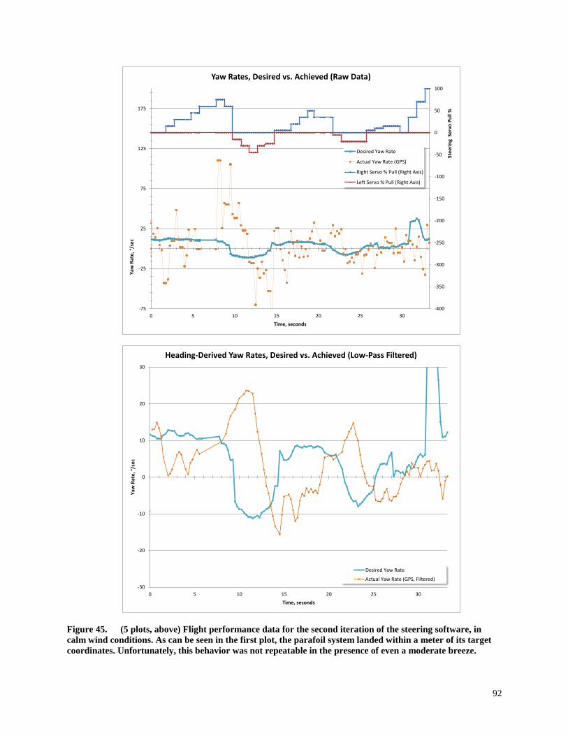
92
Figure 45. (5 plots, above) Flight performance data for the second iteration of the steering software, in
calm wind conditions. As can be seen in the first plot, the parafoil system landed within a meter of its target
coordinates. Unfortunately, this behavior was not repeatable in the presence of even a moderate breeze.
-400
-350
-300
-250
-200
-150
-100
-50
0
50
100
-75
-25
25
75
125
175
0 5 10 15 20 25 30
Ste
eri
ng
Se
rvo
Pu
ll %
Yaw
Rat
e, °
/se
c
Time, seconds
Yaw Rates, Desired vs. Achieved (Raw Data)
Desired Yaw Rate
Actual Yaw Rate (GPS)
Right Servo % Pull (Right Axis)
Left Servo % Pull (Right Axis)
-30
-20
-10
0
10
20
30
0 5 10 15 20 25 30
Yaw
Rat
e, °
/se
c
Time, seconds
Heading-Derived Yaw Rates, Desired vs. Achieved (Low-Pass Filtered)
Desired Yaw Rate
Actual Yaw Rate (GPS, Filtered)
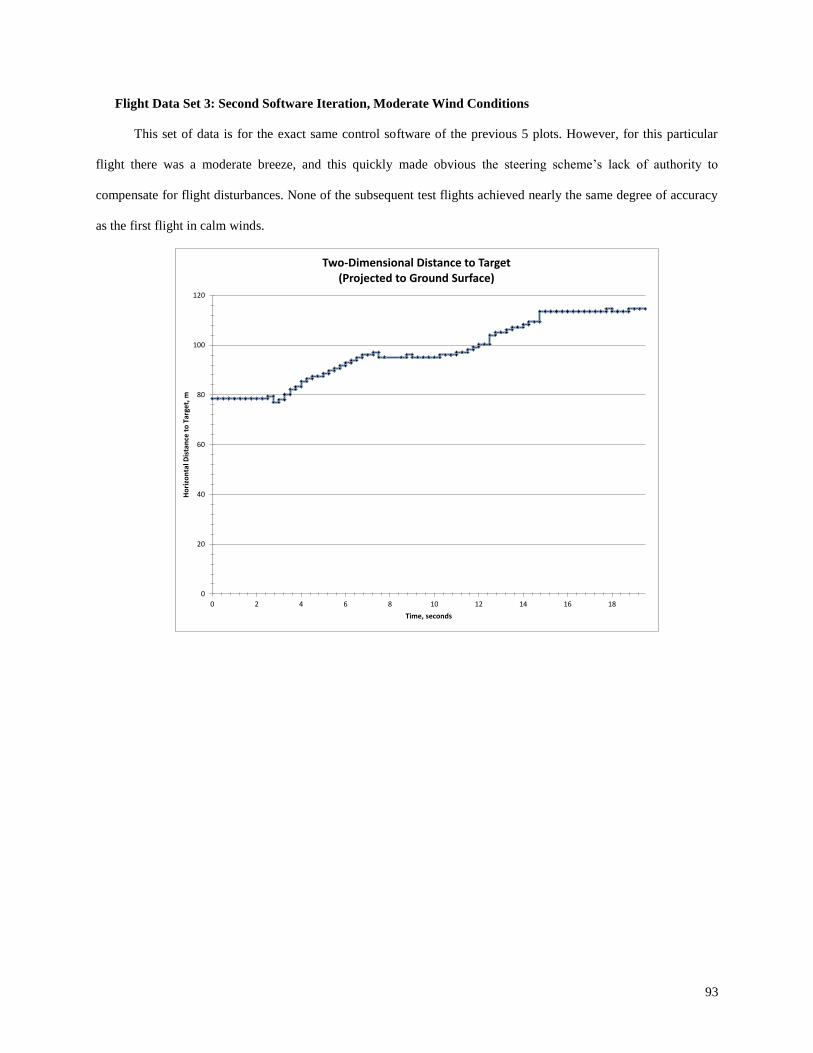
93
Flight Data Set 3: Second Software Iteration, Moderate Wind Conditions
This set of data is for the exact same control software of the previous 5 plots. However, for this particular
flight there was a moderate breeze, and this quickly made obvious the steering scheme’s lack of authority to
compensate for flight disturbances. None of the subsequent test flights achieved nearly the same degree of accuracy
as the first flight in calm winds.
0
20
40
60
80
100
120
0 2 4 6 8 10 12 14 16 18
Ho
rizo
nta
l Dis
tan
ce t
o T
arge
t, m
Time, seconds
Two-Dimensional Distance to Target(Projected to Ground Surface)
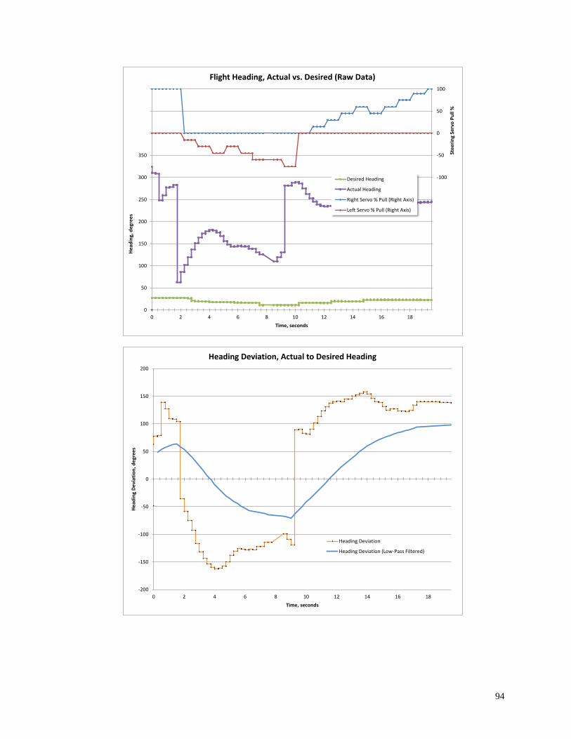
94
-400
-350
-300
-250
-200
-150
-100
-50
0
50
100
0
50
100
150
200
250
300
350
400
450
500
0 2 4 6 8 10 12 14 16 18
Ste
eri
ng
Serv
o P
ull
%
He
adin
g, d
egr
ee
s
Time, seconds
Flight Heading, Actual vs. Desired (Raw Data)
Desired Heading
Actual Heading
Right Servo % Pull (Right Axis)
Left Servo % Pull (Right Axis)
-200
-150
-100
-50
0
50
100
150
200
0 2 4 6 8 10 12 14 16 18
He
adin
g D
evi
atio
n,
de
gre
es
Time, seconds
Heading Deviation, Actual to Desired Heading
Heading Deviation
Heading Deviation (Low-Pass Filtered)
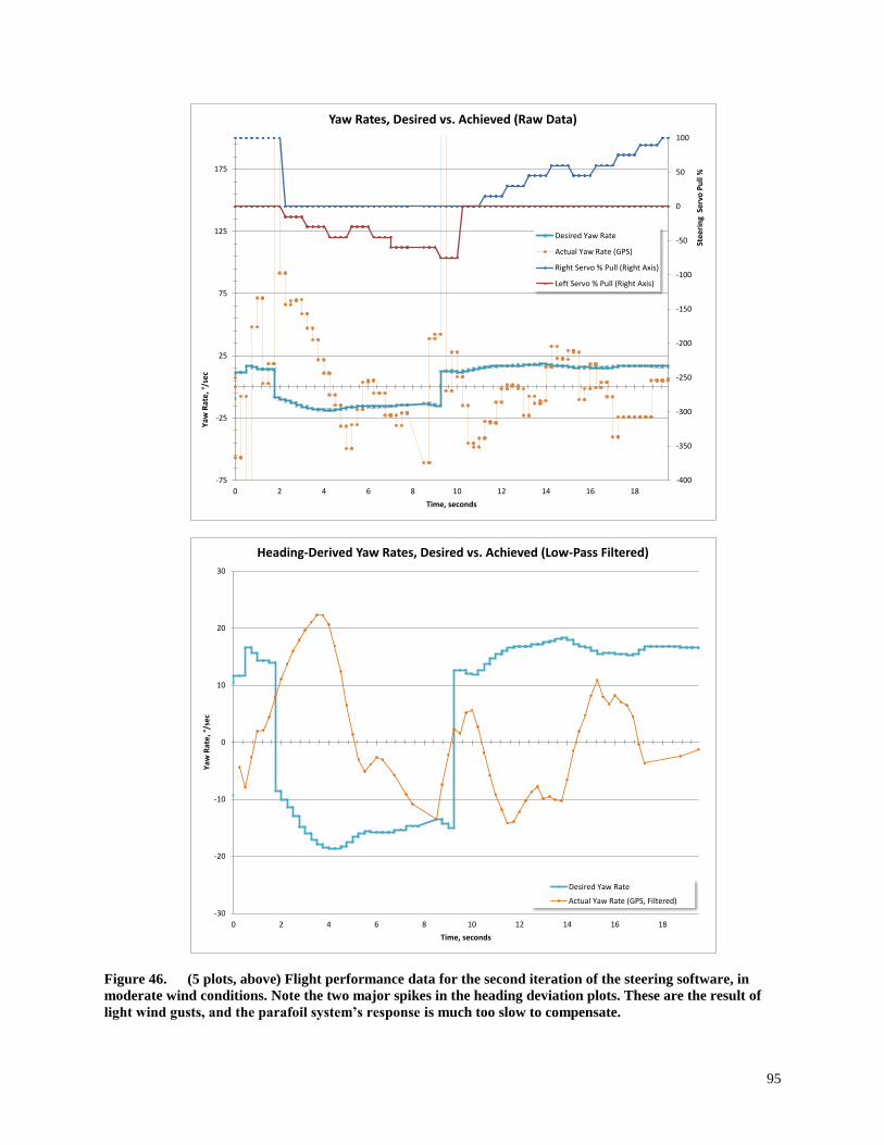
95
Figure 46. (5 plots, above) Flight performance data for the second iteration of the steering software, in
moderate wind conditions. Note the two major spikes in the heading deviation plots. These are the result of
light wind gusts, and the parafoil system’s response is much too slow to compensate.
-400
-350
-300
-250
-200
-150
-100
-50
0
50
100
-75
-25
25
75
125
175
0 2 4 6 8 10 12 14 16 18
Ste
eri
ng
Se
rvo
Pu
ll %
Yaw
Rat
e, °
/se
c
Time, seconds
Yaw Rates, Desired vs. Achieved (Raw Data)
Desired Yaw Rate
Actual Yaw Rate (GPS)
Right Servo % Pull (Right Axis)
Left Servo % Pull (Right Axis)
-30
-20
-10
0
10
20
30
0 2 4 6 8 10 12 14 16 18
Yaw
Rat
e, °
/se
c
Time, seconds
Heading-Derived Yaw Rates, Desired vs. Achieved (Low-Pass Filtered)
Desired Yaw Rate
Actual Yaw Rate (GPS, Filtered)
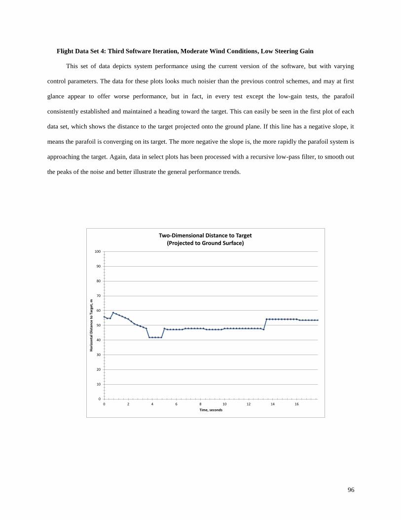
96
Flight Data Set 4: Third Software Iteration, Moderate Wind Conditions, Low Steering Gain
This set of data depicts system performance using the current version of the software, but with varying
control parameters. The data for these plots looks much noisier than the previous control schemes, and may at first
glance appear to offer worse performance, but in fact, in every test except the low-gain tests, the parafoil
consistently established and maintained a heading toward the target. This can easily be seen in the first plot of each
data set, which shows the distance to the target projected onto the ground plane. If this line has a negative slope, it
means the parafoil is converging on its target. The more negative the slope is, the more rapidly the parafoil system is
approaching the target. Again, data in select plots has been processed with a recursive low-pass filter, to smooth out
the peaks of the noise and better illustrate the general performance trends.
0
10
20
30
40
50
60
70
80
90
100
0 2 4 6 8 10 12 14 16
Ho
rizo
nta
l Dis
tan
ce t
o T
arge
t, m
Time, seconds
Two-Dimensional Distance to Target(Projected to Ground Surface)
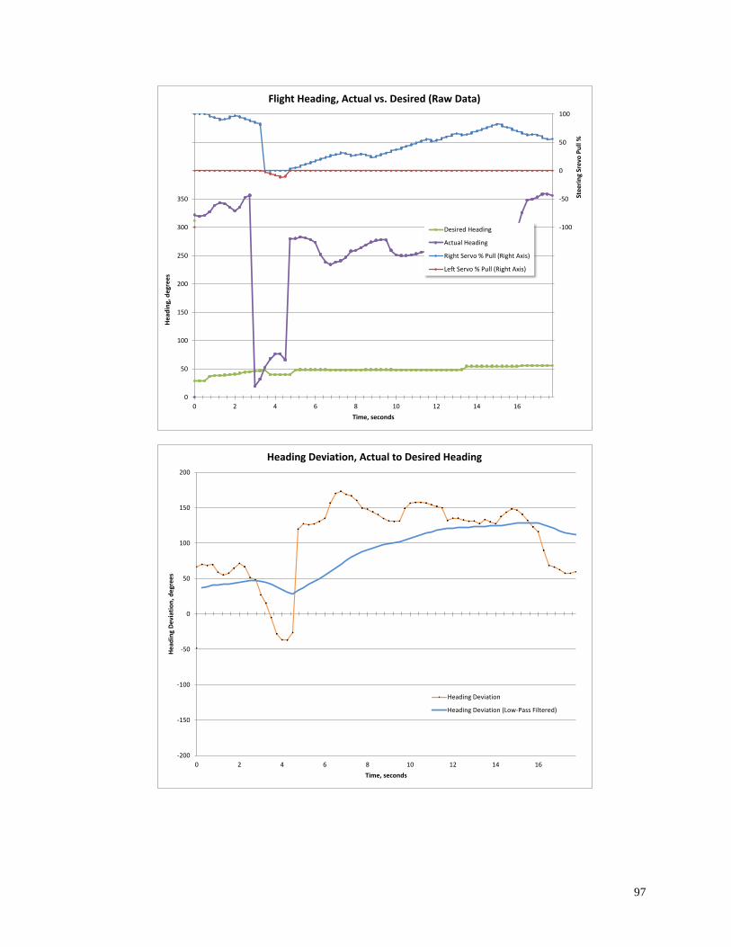
97
-400
-350
-300
-250
-200
-150
-100
-50
0
50
100
0
50
100
150
200
250
300
350
400
450
500
0 2 4 6 8 10 12 14 16
Ste
eri
ng
Sre
vo P
ull
%
He
adin
g, d
egr
ee
s
Time, seconds
Flight Heading, Actual vs. Desired (Raw Data)
Desired Heading
Actual Heading
Right Servo % Pull (Right Axis)
Left Servo % Pull (Right Axis)
-200
-150
-100
-50
0
50
100
150
200
0 2 4 6 8 10 12 14 16
He
adin
g D
evi
atio
n,
de
gre
es
Time, seconds
Heading Deviation, Actual to Desired Heading
Heading Deviation
Heading Deviation (Low-Pass Filtered)
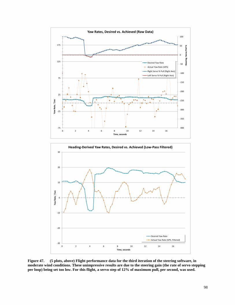
98
Figure 47. (5 plots, above) Flight performance data for the third iteration of the steering software, in
moderate wind conditions. These unimpressive results are due to the steering gain (the rate of servo stepping
per loop) being set too low. For this flight, a servo step of 12% of maximum pull, per second, was used.
-400
-350
-300
-250
-200
-150
-100
-50
0
50
100
-75
-25
25
75
125
175
0 2 4 6 8 10 12 14 16
Ste
eri
ng
Se
rvo
Pu
ll %
Yaw
Rat
e, °
/se
c
Time, seconds
Yaw Rates, Desired vs. Achieved (Raw Data)
Desired Yaw Rate
Actual Yaw Rate (GPS)
Right Servo % Pull (Right Axis)
Left Servo % Pull (Right Axis)
-30
-20
-10
0
10
20
30
0 2 4 6 8 10 12 14 16
Yaw
Rat
e, °
/se
c
Time, seconds
Heading-Derived Yaw Rates, Desired vs. Achieved (Low-Pass Filtered)
Desired Yaw Rate
Actual Yaw Rate (GPS, Filtered)
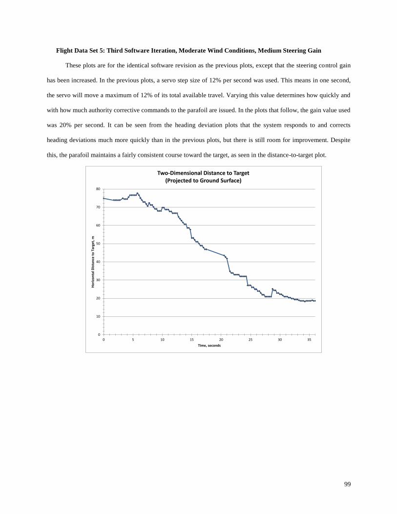
99
Flight Data Set 5: Third Software Iteration, Moderate Wind Conditions, Medium Steering Gain
These plots are for the identical software revision as the previous plots, except that the steering control gain
has been increased. In the previous plots, a servo step size of 12% per second was used. This means in one second,
the servo will move a maximum of 12% of its total available travel. Varying this value determines how quickly and
with how much authority corrective commands to the parafoil are issued. In the plots that follow, the gain value used
was 20% per second. It can be seen from the heading deviation plots that the system responds to and corrects
heading deviations much more quickly than in the previous plots, but there is still room for improvement. Despite
this, the parafoil maintains a fairly consistent course toward the target, as seen in the distance-to-target plot.
0
10
20
30
40
50
60
70
80
0 5 10 15 20 25 30 35
Ho
rizo
nta
l Dis
tan
ce t
o T
arge
t, m
Time, seconds
Two-Dimensional Distance to Target(Projected to Ground Surface)
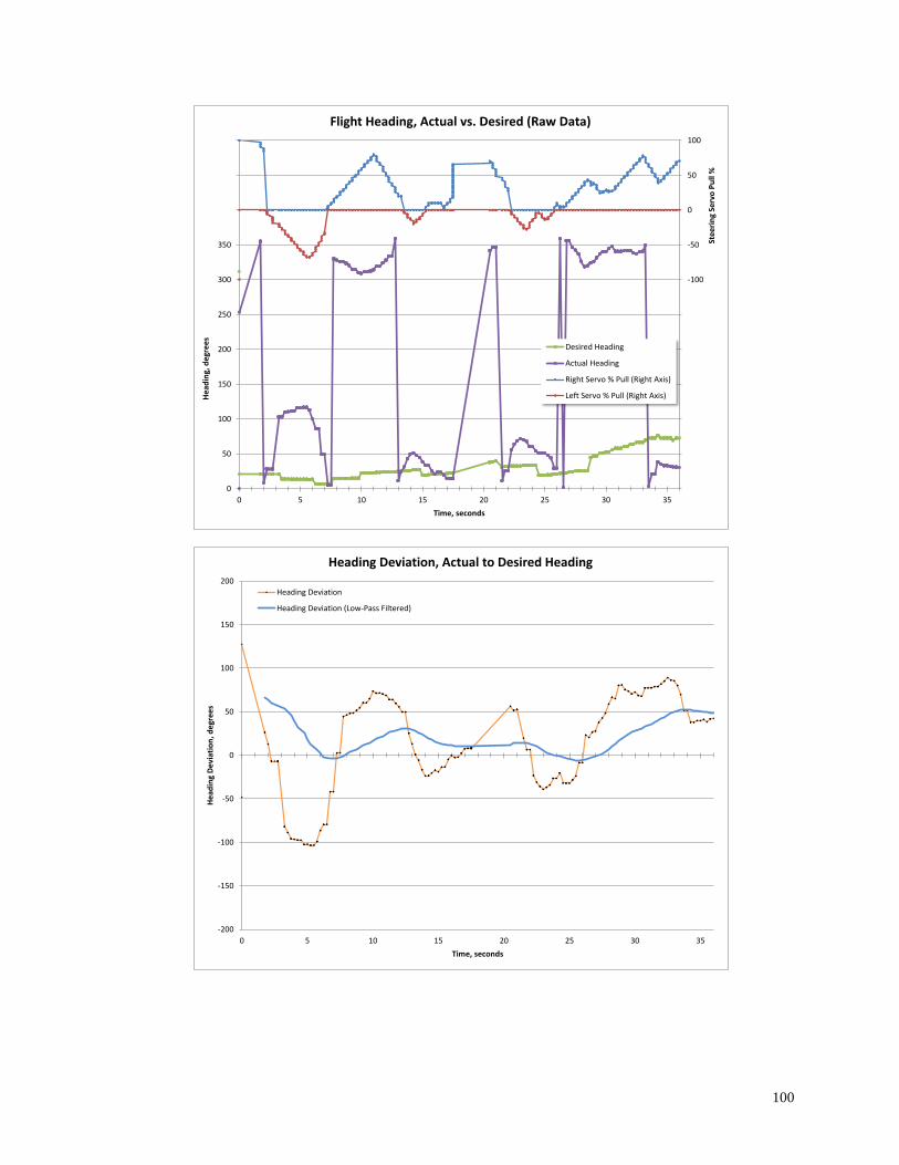
100
-400
-350
-300
-250
-200
-150
-100
-50
0
50
100
0
50
100
150
200
250
300
350
400
450
500
0 5 10 15 20 25 30 35
Ste
eri
ng
Serv
o P
ull
%
He
adin
g, d
egr
ee
s
Time, seconds
Flight Heading, Actual vs. Desired (Raw Data)
Desired Heading
Actual Heading
Right Servo % Pull (Right Axis)
Left Servo % Pull (Right Axis)
-200
-150
-100
-50
0
50
100
150
200
0 5 10 15 20 25 30 35
He
adin
g D
evi
atio
n,
de
gre
es
Time, seconds
Heading Deviation, Actual to Desired Heading
Heading Deviation
Heading Deviation (Low-Pass Filtered)
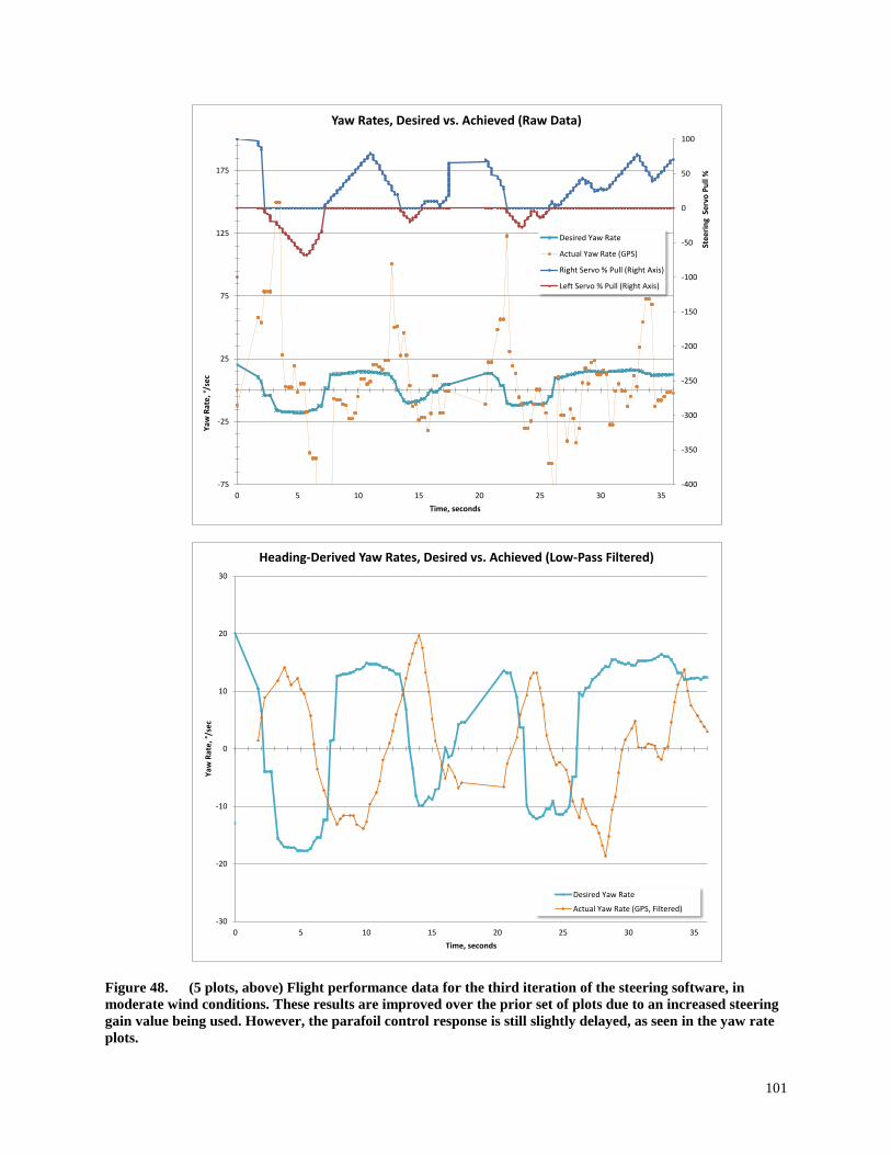
101
Figure 48. (5 plots, above) Flight performance data for the third iteration of the steering software, in
moderate wind conditions. These results are improved over the prior set of plots due to an increased steering
gain value being used. However, the parafoil control response is still slightly delayed, as seen in the yaw rate
plots.
-400
-350
-300
-250
-200
-150
-100
-50
0
50
100
-75
-25
25
75
125
175
0 5 10 15 20 25 30 35
Ste
eri
ng
Se
rvo
Pu
ll %
Yaw
Rat
e, °
/se
c
Time, seconds
Yaw Rates, Desired vs. Achieved (Raw Data)
Desired Yaw Rate
Actual Yaw Rate (GPS)
Right Servo % Pull (Right Axis)
Left Servo % Pull (Right Axis)
-30
-20
-10
0
10
20
30
0 5 10 15 20 25 30 35
Yaw
Rat
e, °
/se
c
Time, seconds
Heading-Derived Yaw Rates, Desired vs. Achieved (Low-Pass Filtered)
Desired Yaw Rate
Actual Yaw Rate (GPS, Filtered)
102
Flight Data Set 6: Third Software Iteration, Moderate Wind Conditions, Medium-High Steering Gain
These plots show the performance results of the parafoil system under identical conditions to the prior sets,
except that the gain has again been increased, to a value of 30% servo pull per second. In this test, the parafoil
system was so efficient in its steering processes (that is, not losing most of its altitude to major steering corrections
as in previous tests) that it arrived into the landing threshold with substantial altitude remaining. Unfortunately, the
landing threshold radius was specified much too small due to the limited size of the test area and the limited altitude
available for descent. Because of this, the parafoil entered the landing circle threshold and immediately gave strong
input for the landing spiral, but the inertial lag of the parafoil system changing course was too great and the system
exited the other side of the landing circle. (In fact, in the flight video, it can be seen that the parafoil turns nearly
180° upon entering the landing circle, but then flies backwards for a short distance until it exits the landing circle
threshold.) After exiting the landing threshold, the parafoil system managed to again orient itself to the target, re-
enter the landing threshold, and again flew through it, this time running out of altitude and landing. This is very
impressive performance when compared to the behavior of the prior system tests with the previous software
iterations.
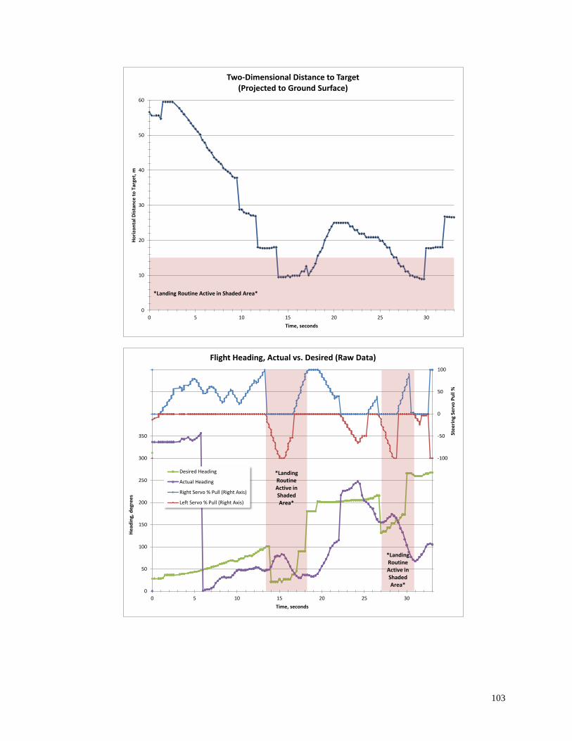
103
0
10
20
30
40
50
60
0 5 10 15 20 25 30
Ho
rizo
nta
l Dis
tan
ce t
o T
arge
t, m
Time, seconds
Two-Dimensional Distance to Target(Projected to Ground Surface)
*Landing Routine Active in Shaded Area*
-400
-350
-300
-250
-200
-150
-100
-50
0
50
100
0
50
100
150
200
250
300
350
400
450
500
0 5 10 15 20 25 30
Ste
eri
ng
Serv
o P
ull
%
He
adin
g, d
egr
ee
s
Time, seconds
Flight Heading, Actual vs. Desired (Raw Data)
Desired Heading
Actual Heading
Right Servo % Pull (Right Axis)
Left Servo % Pull (Right Axis)
*LandingRoutine Active in Shaded Area*
*LandingRoutine Active in Shaded Area*
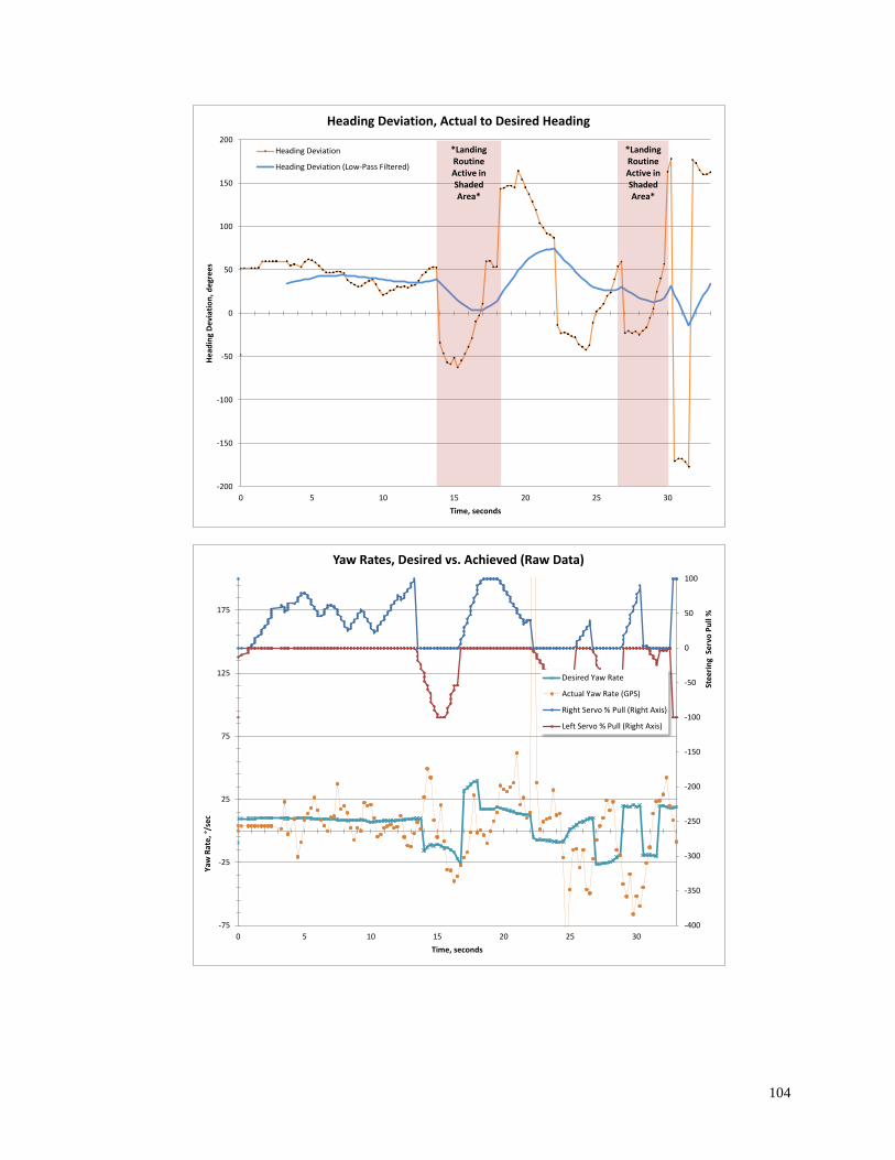
104
-200
-150
-100
-50
0
50
100
150
200
0 5 10 15 20 25 30
He
adin
g D
evi
atio
n,
de
gre
es
Time, seconds
Heading Deviation, Actual to Desired Heading
Heading Deviation
Heading Deviation (Low-Pass Filtered)
*LandingRoutine Active in Shaded Area*
*LandingRoutine Active in Shaded Area*
-400
-350
-300
-250
-200
-150
-100
-50
0
50
100
-75
-25
25
75
125
175
0 5 10 15 20 25 30
Ste
eri
ng
Se
rvo
Pu
ll %
Yaw
Rat
e, °
/se
c
Time, seconds
Yaw Rates, Desired vs. Achieved (Raw Data)
Desired Yaw Rate
Actual Yaw Rate (GPS)
Right Servo % Pull (Right Axis)
Left Servo % Pull (Right Axis)
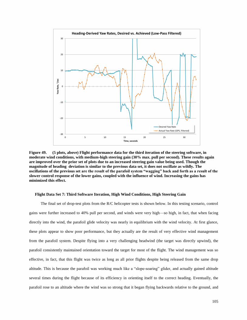
105
Figure 49. (5 plots, above) Flight performance data for the third iteration of the steering software, in
moderate wind conditions, with medium-high steering gain (30% max. pull per second). These results again
are improved over the prior set of plots due to an increased steering gain value being used. Though the
magnitude of heading deviation is similar to the previous data set, it does not oscillate as wildly. The
oscillations of the previous set are the result of the parafoil system “wagging” back and forth as a result of the
slower control response of the lower gains, coupled with the influence of wind. Increasing the gains has
minimized this effect.
Flight Data Set 7: Third Software Iteration, High Wind Conditions, High Steering Gain
The final set of drop-test plots from the R/C helicopter tests is shown below. In this testing scenario, control
gains were further increased to 40% pull per second, and winds were very high—so high, in fact, that when facing
directly into the wind, the parafoil glide velocity was nearly in equilibrium with the wind velocity. At first glance,
these plots appear to show poor performance, but they actually are the result of very effective wind management
from the parafoil system. Despite flying into a very challenging headwind (the target was directly upwind), the
parafoil consistently maintained orientation toward the target for most of the flight. The wind management was so
effective, in fact, that this flight was twice as long as all prior flights despite being released from the same drop
altitude. This is because the parafoil was working much like a “slope-soaring” glider, and actually gained altitude
several times during the flight because of its efficiency in orienting itself to the correct heading. Eventually, the
parafoil rose to an altitude where the wind was so strong that it began flying backwards relative to the ground, and
-30
-20
-10
0
10
20
30
0 5 10 15 20 25 30
Yaw
Rat
e, °
/se
c
Time, seconds
Heading-Derived Yaw Rates, Desired vs. Achieved (Low-Pass Filtered)
Desired Yaw Rate
Actual Yaw Rate (GPS, Filtered)
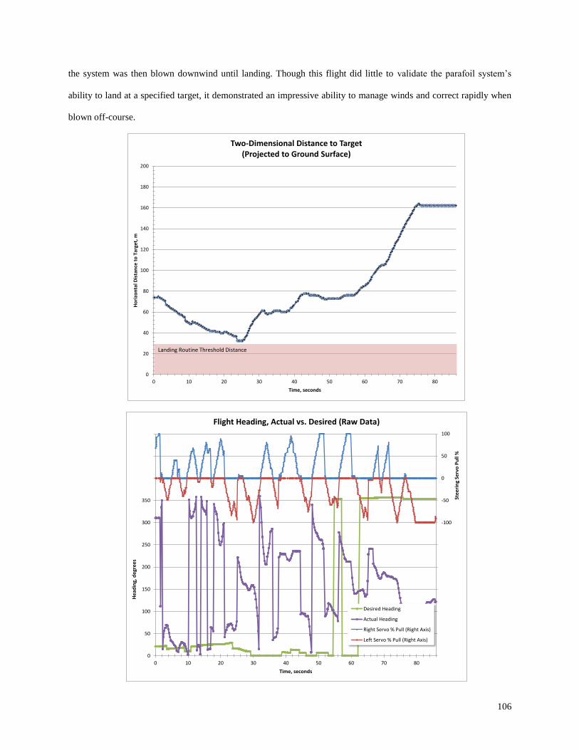
106
the system was then blown downwind until landing. Though this flight did little to validate the parafoil system’s
ability to land at a specified target, it demonstrated an impressive ability to manage winds and correct rapidly when
blown off-course.
0
20
40
60
80
100
120
140
160
180
200
0 10 20 30 40 50 60 70 80
Ho
rizo
nta
l Dis
tan
ce t
o T
arge
t, m
Time, seconds
Two-Dimensional Distance to Target(Projected to Ground Surface)
Landing Routine Threshold Distance
-400
-350
-300
-250
-200
-150
-100
-50
0
50
100
0
50
100
150
200
250
300
350
400
450
500
0 10 20 30 40 50 60 70 80
Ste
eri
ng
Serv
o P
ull
%
He
adin
g, d
egr
ee
s
Time, seconds
Flight Heading, Actual vs. Desired (Raw Data)
Desired Heading
Actual Heading
Right Servo % Pull (Right Axis)
Left Servo % Pull (Right Axis)
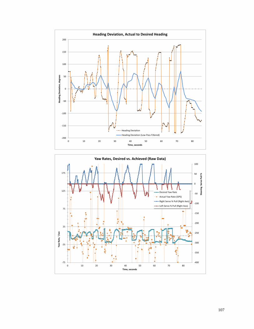
107
-200
-150
-100
-50
0
50
100
150
200
0 10 20 30 40 50 60 70 80
He
adin
g D
evi
atio
n,
de
gre
es
Time, seconds
Heading Deviation, Actual to Desired Heading
Heading Deviation
Heading Deviation (Low-Pass Filtered)
-400
-350
-300
-250
-200
-150
-100
-50
0
50
100
-75
-25
25
75
125
175
0 10 20 30 40 50 60 70 80
Ste
eri
ng
Se
rvo
Pu
ll %
Yaw
Rat
e, °
/se
c
Time, seconds
Yaw Rates, Desired vs. Achieved (Raw Data)
Desired Yaw Rate
Actual Yaw Rate (GPS)
Right Servo % Pull (Right Axis)
Left Servo % Pull (Right Axis)
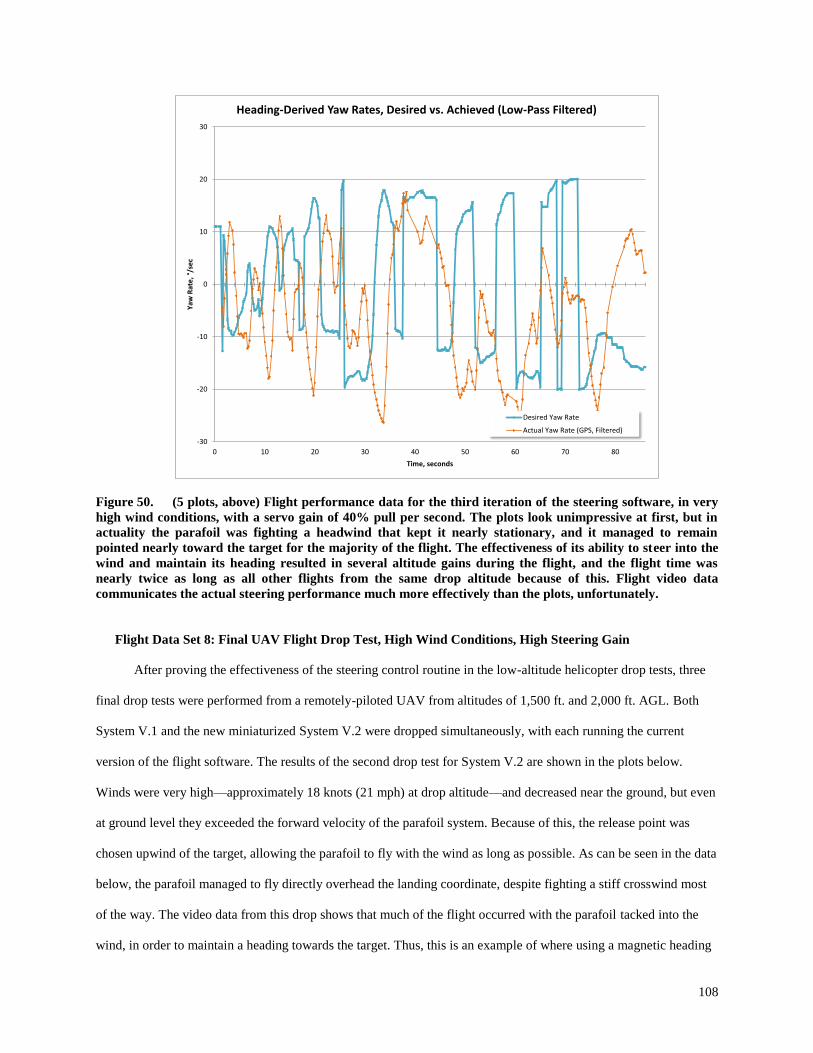
108
Figure 50. (5 plots, above) Flight performance data for the third iteration of the steering software, in very
high wind conditions, with a servo gain of 40% pull per second. The plots look unimpressive at first, but in
actuality the parafoil was fighting a headwind that kept it nearly stationary, and it managed to remain
pointed nearly toward the target for the majority of the flight. The effectiveness of its ability to steer into the
wind and maintain its heading resulted in several altitude gains during the flight, and the flight time was
nearly twice as long as all other flights from the same drop altitude because of this. Flight video data
communicates the actual steering performance much more effectively than the plots, unfortunately.
Flight Data Set 8: Final UAV Flight Drop Test, High Wind Conditions, High Steering Gain
After proving the effectiveness of the steering control routine in the low-altitude helicopter drop tests, three
final drop tests were performed from a remotely-piloted UAV from altitudes of 1,500 ft. and 2,000 ft. AGL. Both
System V.1 and the new miniaturized System V.2 were dropped simultaneously, with each running the current
version of the flight software. The results of the second drop test for System V.2 are shown in the plots below.
Winds were very high—approximately 18 knots (21 mph) at drop altitude—and decreased near the ground, but even
at ground level they exceeded the forward velocity of the parafoil system. Because of this, the release point was
chosen upwind of the target, allowing the parafoil to fly with the wind as long as possible. As can be seen in the data
below, the parafoil managed to fly directly overhead the landing coordinate, despite fighting a stiff crosswind most
of the way. The video data from this drop shows that much of the flight occurred with the parafoil tacked into the
wind, in order to maintain a heading towards the target. Thus, this is an example of where using a magnetic heading
-30
-20
-10
0
10
20
30
0 10 20 30 40 50 60 70 80
Yaw
Rat
e, °
/se
c
Time, seconds
Heading-Derived Yaw Rates, Desired vs. Achieved (Low-Pass Filtered)
Desired Yaw Rate
Actual Yaw Rate (GPS, Filtered)

109
alone for steering would prove ineffective, as the parafoil had to be oriented pointing slightly away from the target
in order to actually reach it. After arriving at the target, the parafoil entered the landing routine, and managed to
successfully perform two complete spirals above the target coordinates. Furthermore, the data log shows that the
landing spiral size achieved was almost exactly the size specified in the software (17 m). However, the strong
prevailing winds eventually forced the parafoil beyond the target coordinate. Once the parafoil was downwind of the
target, it became impossible to approach it again, because the winds exceeded the forward glide velocity of the
parafoil. Despite this, the system continued to attempt to orient itself toward the target, and landed less than 100 m
from the target while facing directly toward it.
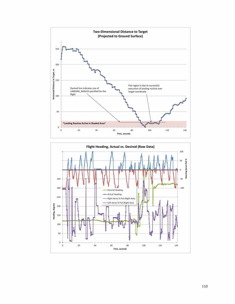
110
0
50
100
150
200
250
0 20 40 60 80 100 120 140
Ho
rizo
nta
l Dis
tan
ce t
o T
arge
t, m
Time, seconds
Two-Dimensional Distance to Target(Projected to Ground Surface)
*Landing Routine Active in Shaded Area*
Flat region is due to successful execution of landing routine over target coordinate
Dashed line indicates size of LANDING_RADIUS specified for the flight
-400
-350
-300
-250
-200
-150
-100
-50
0
50
100
0
50
100
150
200
250
300
350
400
450
500
0 20 40 60 80 100 120 140
Ste
eri
ng
Serv
o P
ull
%
He
adin
g, d
egr
ee
s
Time, seconds
Flight Heading, Actual vs. Desired (Raw Data)
Desired Heading
Actual Heading
Right Servo % Pull (Right Axis)
Left Servo % Pull (Right Axis)
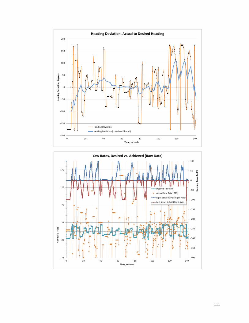
111
-200
-150
-100
-50
0
50
100
150
200
0 20 40 60 80 100 120 140
He
adin
g D
evi
atio
n,
de
gre
es
Time, seconds
Heading Deviation, Actual to Desired Heading
Heading Deviation
Heading Deviation (Low-Pass Filtered)
-400
-350
-300
-250
-200
-150
-100
-50
0
50
100
-75
-25
25
75
125
175
0 20 40 60 80 100 120 140
Ste
eri
ng
Se
rvo
Pu
ll %
Yaw
Rat
e, °
/se
c
Time, seconds
Yaw Rates, Desired vs. Achieved (Raw Data)
Desired Yaw Rate
Actual Yaw Rate (GPS)
Right Servo % Pull (Right Axis)
Left Servo % Pull (Right Axis)
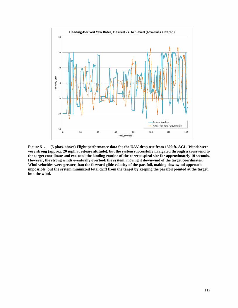
112
Figure 51. (5 plots, above) Flight performance data for the UAV drop test from 1500 ft. AGL. Winds were
very strong (approx. 20 mph at release altitude), but the system successfully navigated through a crosswind to
the target coordinate and executed the landing routine of the correct spiral size for approximately 10 seconds.
However, the strong winds eventually overtook the system, moving it downwind of the target coordinates.
Wind velocities were greater than the forward glide velocity of the parafoil, making downwind approach
impossible, but the system minimized total drift from the target by keeping the parafoil pointed at the target,
into the wind.
-30
-20
-10
0
10
20
30
0 20 40 60 80 100 120 140
Yaw
Rat
e, °
/se
c
Time, seconds
Heading-Derived Yaw Rates, Desired vs. Achieved (Low-Pass Filtered)
Desired Yaw Rate
Actual Yaw Rate (GPS, Filtered)
113
VII. Discussion and Future Work
As illustrated by the plots of the preceding section, through a number of iterations and refinements to the control
algorithm, a solution has been reached which reliably and consistently guides the parafoil system to a predefined
target. In manageable winds, the system performs very well, and has demonstrated the ability to maintain a precise
heading even when tacked into the wind. The limitations of the system are reached when wind velocities exceed the
parafoil system’s ability to fly upwind, which is a scenario that can be largely mitigated through intelligent mission
planning.
The System V.2 device has demonstrated a high degree of capability in its current form, but there is room left for
exciting future improvements. With an effective steering control algorithm already developed, it becomes a fairly
simple matter to add improved guidance logic, which includes the ability to manage strong winds from an upwind
approach by shedding excess altitude prior to arriving at the target. Also, an implementation of the IMU’s
magnetometer heading used in conjunction with the GPS heading can eliminate the issue of unnecessary turning
while drifting backward in strong headwinds.
Future work for the parafoil system as a whole, applied to SPQR, includes the development of both the parafoil
deployment system, and a compact, deployable means to assist the parafoil with rapid inflation at high altitudes. An
inflatable variant of the carbon-fiber cross structure discussed previously may provide the solution to the latter, and
the compact design of System V.2 ensures feasibility of the former. In regards to other applications, the potential for
a parafoil system to return high-altitude balloon payloads to a target location is extremely attractive, and may well
prove to be the nearest future implementation of the technology.
114
VIII. Conclusion
A small autonomous parafoil system has been developed, compatible in size, shape, mass, and general operation
with the ISS on-demand sample return concept SPQR (Small Payload Quick-Return). The parafoil system has been
optimized with regard to structural efficiency, and has simultaneously incorporated design refinements that reduce
complexity, improve reliability, and minimize potential failure modes. Custom control software for the parafoil
system has proven effective in a range of flight tests, demonstrating a consistent ability to guide the device to a
predefined set of target coordinates, even in the presence of moderate crosswinds. In addition, the parafoil system
has been designed with its intended application to spaceflight payloads in mind, reducing the extent of future design
revision required to bring the device to a spaceflight-ready level of development. While primarily intended to fill the
role of a terminal descent recovery device for SPQR, many other attractive applications of the technology exist at a
range of scales, from payload return for amateur high-altitude balloon experiments, to the targeted delivery of sub-
orbital sounding rocket payloads.
115
IX. References
1Murbach, M.S., Boronowsky, K.M., and Benton, J.E., et al. "Options for Returning Payloads from the ISS after the
Termination of STS Flights," 40th International Conference on Environmental Systems, American Institute of Aeronautics and
Astronautics, 2010.
2Arves, J., Gnau, M., et al. “Overview of the Hybrid Sounding Rocket (HYSR) Project.” 39th AIAA/ASME/SAE/ASEE Joint
Propulsion Conference and Exhibit, Huntsville, Alabama, 20-23 July 2003.
3"Parachute," Wikipedia. [http://en.wikipedia.org/wiki/Parachute. Accessed 10/6/2011.]
4United States National Reconnaissance Office. “The CORONA Story.” Declassified/Approved for Release 30 June 2010.
5GlobalSecurity.org. “Joint Precision Airdrop System [JPADS].”
[http://www.globalsecurity.org/military/systems/aircraft/systems/jpads.htm. Accessed 10/6/2011.]
6Slegers, N.J. and Yakimenko, O.A., “Optimal Control for Terminal Guidance of Autonomous Parafoils.” 20th AIAA
Aerodynamic Decelerator Systems Technology Conference and Seminar, Seattle, Washington, 4 - 7 May 2009.
7Yakimenko, O. A., Slegers, N. J., and Tiaden, R.A. “Development and Testing of the Miniature Aerial Delivery System
Snowflake.” 20th AIAA Aerodynamic Decelerator Systems Technology Conference and Seminar, Seattle, Washington, 4 - 7
May 2009.
8 Naval Postgraduate School Aerodynamic Decelerator Systems Center (ADSC). “Snowflake.”
[http://www.nps.edu/Academics/Centers/ADSC/Projects/Snowflake/SnowflakeSystem.html. Accessed 10/6/2011.]
9Zuniga, D., Murbach, M., Leimkuehler, T., Leidich, J., Chiesi, S., “Conceptual Development of a Payload Thermal and
Pressure Control System for a Small Payload Quick Return Vehicle,” 40th International Conference on Environmental Systems,
Barcelona, Spain, July 11-15, 2010, AIAA-2010-6222.
10MMIST. “Sherpa Provider” (online product brochure).
[http://mmist.ca/Media/Docs/Brochures/Sherpa_Provider_Brochure.pdf. Cited 20 November 2011.]

116
Appendix A
Complete Flight Software
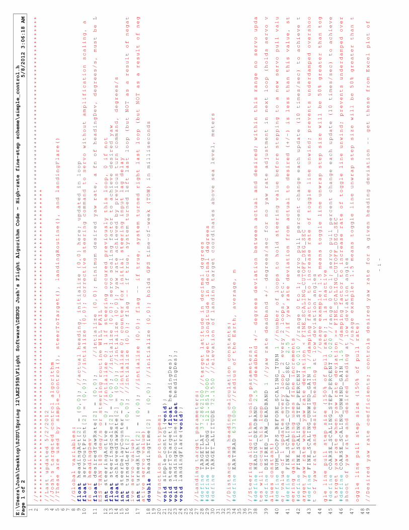
E:\Users\Josh\Desktop\SJSU\Spring 12\AE295B\Flight Software\DEBUG Josh's Flight Algorithm Code - High-rate fine-step scheme\simple_control.h
Page 1 of 2
5/8/2012 3:06:18 AM
1
2 //***********************************************************************************************************************
******************************************************************************
3 //Last updated 5/2/2012
4 //Josh's targeted control algorithm
5 //These are used by simple_control(), steerToTarget(), landingRoutine(), and landingFlare()
6
7
8 //Global variables:
9 float headingAct[2] = {0,0}; //actual heading, initialize {0,0} here; updated in loop
10 float servoOutPrcnt[2] = {0,0}; //intialize {0,0}; corrective steering command to servo without amplification scaling, a
fn of headingDev
11 float desiredYawRate[2] = {0,0}; //intialize {0,0}; minimum desired yaw rate, a fn of headingDev, degrees/s, must be L
ESS THAN 180 deg/s or steering routine WILL FAIL
12 int steeringActive = 0; //intialize 0; 1 if steering occured previously this loop, 0 if not
13 float steeringScale[2] = {0,0}; //intialize {0,0}; servo scaling factor to achieve desired yaw
14 float achievedYawRate[2] = {0.0}; //intialize {0,0}; yaw rate achieved by previous turn command, degrees/s
15 int steerDelayCounter = 0; //intialize 0; counter for initial steering input lag delay
16 int turnedLeft[2] = {0,0}; //intialize {0,0}; flag -- if true, system turned left last loop (but NOT as a result of negat
ive servo value)
17 int turnedRight[2] = {0,0}; //intialize {0,0}; flag -- if true, system turned right last loop (but NOT as a result of neg
ative servo value)
18 double headingTime[2] = {0,0}; //initialize {0,0}; holds GPS time-of-week (TOW) in milliseconds
19
20 //Function prototypes:
21 void simple_control(void);
22 void steerToTarget(float headingDes);
23 void landingRoutine(float headingDes);
24 void landingFlare(void);
25
26
27 //Landing target parameters:
28 #define TARGETLAT 37.2862100 //target latitude in decimal degrees
29 #define TARGETLONG -121.8517000 //target longitude in decimal degrees
30 #define TARGET_ALTITUDE 72.1550 //elevation of landing target coordinates above sea level, meters
31
32
33 //Distance and heading calculation constants:
34 #define EARTHRAD 6371000 //radius of the Earth, average, m
35
36
37 //Steering algorithm tuning parameters:
38 #define HEADING_DEADBAND 2.5 //deadband +/- degrees deviation between actual and desired; within this range no servo upda
tes will occur this loop
39 #define DESIRED_YAW_DEADBAND 1 //yaw rate deadband +/- degrees/sec for no yaw rate adjustment in next loop (holds servo v
alues constant)
40 #define NUM_LOOPS_BEFORE_SCALING_TURN 1 //number of loops to hold steering value before stepping to a new servo pull valu
e; value of 1 updates every loop, 2 every 2 loops, etc.
41 #define FINE_SCALING_CUTOFF_DEG_SEC 2.5 //if yaw rate deviation from actual to desired (+/-) is less than this value, st
eering gain stepping uses fine increments
42 #define FINE_SCALING_STEP_PERCENT 0.010 //range 0 to 1; servo pull percent change each update (10 times/sec) to achieve t
arget yaw rate when yaw rate deviation < FINE_SCALING_CUTOFF_DEG_SEC
43 #define FINE_SCALING_UNWIND_GAIN 1 //damping factor to increase rate of toggle line unwind; prevents underdamped overshoo
t of yaw rate and desired heading at low deviation angles
44 //usage example: 1.5 means toggle line unwrap step size will be 50% greater than tog
gle line pull step size (150% of pull rate); 1 is inactive
45 #define COARSE_SCALING_STEP_PERCENT 0.020 //range 0 to 1; servo pull percent change each update (10 times/sec) to achieve
target yaw rate when yaw rate deviation >= FINE_SCALING_CUTOFF_DEG_SEC
46 #define COARSE_SCALING_UNWIND_GAIN 1.5 //damping factor to increase rate of toggle line unwind; prevents underdamped over
shoot of yaw rate and desired heading at low deviation angles
47 //usage example: 1.5 means toggle line unwrap step size will be 50% greater than t
oggle line pull step size (150% of pull rate)
48
49 //Desired yaw rate coefficients; controls desired yaw rate for a given heading deviation -- get these from Excel plot of
- 1 -
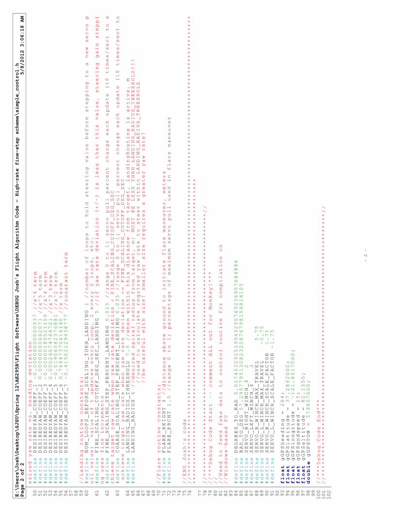
E:\Users\Josh\Desktop\SJSU\Spring 12\AE295B\Flight Software\DEBUG Josh's Flight Algorithm Code - High-rate fine-step scheme\simple_control.h
Page 2 of 2
5/8/2012 3:06:18 AM
esired yaw rate vs. heading deviation
50
#define DESIREDYAW_COEFF_1 -0.00000000000937 //x^6 term
51
#define DESIREDYAW_COEFF_2 0.00000000662071 //x^5 term
52
#define DESIREDYAW_COEFF_3 -0.00000185521159 //x^4 term
53
#define DESIREDYAW_COEFF_4 0.00026074766721 //x^3 term
54
#define DESIREDYAW_COEFF_5 -0.01906582376881 //x^2 term
55
#define DESIREDYAW_COEFF_6 0.76467370416140 //x term
56
#define DESIREDYAW_COEFF_7 -0.41502129438777 //constant term
57
58
59
//Landing routine constants:
60
#define NUM_LOOPS_BEFORE_SCALING_TURN_LANDING 1 //number of loops to hold steering value before stepping to a new servo p
ull value; value of 1 updates every loop, 2 every 2 loops, etc.
61
#define FINE_SCALING_CUTOFF_DEG_SEC_LANDING 5 //if yaw rate deviation (+/-) is less than this value, steering gain steppi
ng uses fine increments
62
#define FINE_SCALING_STEP_PERCENT_LANDING 0.015 //range 0 to 1; servo pull percent change each update (10 times/sec) to a
chieve target yaw rate when yaw rate deviation < FINE_SCALING_CUTOFF_DEG_SEC
63
#define COARSE_SCALING_STEP_PERCENT_LANDING 0.035 //range 0 to 1; servo pull percent change each update (10 times/sec) to
achieve target yaw rate when yaw rate deviation >= FINE_SCALING_CUTOFF_DEG_SEC
64
#define LANDING_RADIUS_THRESHOLD 7.5 //when within this distance from target, landingRoutine is active, m
65
#define LANDING_RADIUS 6 //desired spiral radius from target, m; MUST BE LESS THAN LANDING_RADIUS_THRESHOLD!!!
66
//used to calculate required yaw rate to steer within LANDING_RADIUS_THRESHOLD
67
//be careful with size! smaller size requires a greater yaw rate!
68
69
70
//Flare routine constants:
71
#define FLARE_HEIGHT 4 //distance above ground to initiate flare maneuver, meters
72
#define FLARE_PRCNT 1.0 //range 0 to 1; percentage of maximum servo pull used in flare maneuver
73
74
75
//END Josh's code
76
//***********************************************************************************************************************
*******************************************************************************
77
78
//********************************************************************//
79
//***Debug Code Start -- comment ALL out for Monkey!***
80
//
81
//Used to feed fake data to control routine for compilation on
82
//Windows-based PC
83
84
#define DEGREES_TO_RAD 0.017453292519943295769236907684886
85
#define RAD_TO_DEG 57.295779513082320876798154814105
86
#define SERVO_RIGHT_WINCH_3 2
87
#define SERVO_LEFT_WINCH_4 3
88
#define SERVO_R_WINCH_MAX_TRAVEL 5.75
89
#define SERVO_L_WINCH_MAX_TRAVEL -5.75
90
#define SERVO_R_WINCH_SCALE_FACTOR 1.75
91
#define SERVO_L_WINCH_SCALE_FACTOR -1.75
92
93
float gGPSheading = 284;
94
float gGPSlatitude = 37.2862000;
95
float gGPSlongitude = -121.8517000;
96
float gGPSgndspeed = 15;
97
float gGPSaltitude = 82.1550;
98
double gGPSTOW = 579857000;
99
100
//***Debug Code End***
101
//********************************************************************//
102
- 2 -
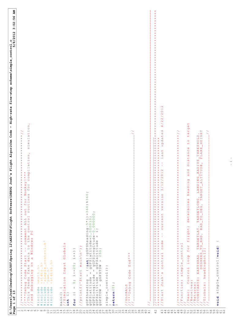
E:\Users\Josh\Desktop\SJSU\Spring 12\AE295B\Flight Software\DEBUG Josh's Flight Algorithm Code - High-rate fine-step scheme\simple_control.c
Page 1 of 13
5/8/2012 3:02:56 AM
1
2 //********************************************************************//
3 //***Debug Code Start -- comment ALL out for Monkey!***
4 //This feeds fake data to the control routines for compilation, simulation,
5 //and debugging on a Windows PC
6
7 #include <math.h>
8 #include <stdio.h>
9 #include "simple_control.h"
10 #include "pwm.h"
11 #include <stdlib.h>
12
13
14 main() {
15 //Simulation Input Globals
16 int i;
17
18 for (i = 0; i<=20; i++){
19
20 //printf("Start main\n");
21
22 gGPSheading = ((int)(gGPSheading-5*i)+360)%360;
23 gGPSlatitude = gGPSlatitude+0.000010;
24 gGPSlongitude = gGPSlongitude-0.000000;
25 gGPSaltitude = gGPSaltitude + i;
26 gGPSTOW = gGPSTOW + 250;
27
28 simple_control();
29 }
30 return(0);
31 }
32
33
34 //GLOBALS
35 //***Debug Code End***
36 //____________________________________________________________________//
37
38
39
40
41 //_______________________________________________________________________________________________________________________
_____________________________________________________________________
42 //***********************************************************************************************************************
*********************************************************************
43 //Start Josh's control code -- current version 3/12/2012 -- last updated 4/22/2012
44
45
46
47
48 //********************************************************************//
49 //Function: simple_control
50 //
51 //Desc: Control loop for flight; determines heading and distance to target
52 //Receives:
53 //Returns:
54 //CONSTANTS: EARTHRAD, TARGETLAT, TARGETLONG, LANDING_RADIUS_THRESHOLD,
55 // DEGREES_TO_RAD, RAD_TO_DEG, TARGET_ALTITUDE, FLARE_HEIGHT
56 //Globals: headingAct[2]
57 //____________________________________________________________________//
58
59
60 void simple_control(void) {
61
62
- 1 -
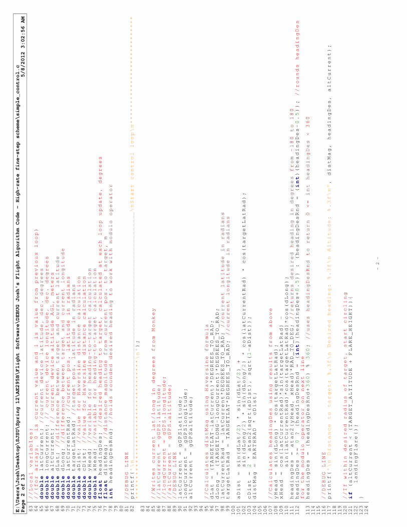
E:\Users\Josh\Desktop\SJSU\Spring 12\AE295B\Flight Software\DEBUG Josh's Flight Algorithm Code - High-rate fine-step scheme\simple_control.c
Page 2 of 13
5/8/2012 3:02:56 AM
63
//Local variables:
64
//(for arrays, 0 is current value and 1 is value from previous loop)
65
double latCurrent; //current device latitude, dec. degrees
66
double longCurrent; // current device longitude, dec. degrees
67
double altCurrent; // current device altitude AGL, meters
68
double dLat; //difference between target and current latitude
69
double dLong; //difference between target and current longitude
70
double latCurrentRad; //current pos. latitude in radians
71
double targetLatRad; //target pos. latitude in radians
72
double aDist; //value for Haversine distance calculation
73
double cDist; //value for Haversine distance calculation
74
double yHead; //variable for heading-to-target calculation
75
double xHead; //variable for heading-to-target calculation
76
float headingDes; //desired heading to target, calculated at each loop update, degrees
77
float distMag; //distance magnitude from current pos. to target, m
78
int headingDesRnd; //holds rounded desired heading to work with modulo operator
79
80
81
//DEBUG LINE
82
printf("\n______________________________________________________________\nStart control loop\n***************************
***********************************\n");
83
84
85
//Writes current lat/long in degrees from Monkey
86
//latCurrent = gGPS.latitude;
87
//longCurrent = gGPS.longitude;
88
//altCurrent = gGPS.altitude;
89
//DEBUG LINE
90
latCurrent = gGPSlatitude;
91
longCurrent = gGPSlongitude;
92
altCurrent = gGPSaltitude;
93
94
95
//Calculates distMag using Haversine formula
96
dLat = (TARGETLAT-latCurrent)*DEGREES_TO_RAD;
97
dLong = (TARGETLONG-longCurrent)*DEGREES_TO_RAD;
98
latCurrentRad = latCurrent*DEGREES_TO_RAD; //current latitude in radians
99
targetLatRad = TARGETLAT*DEGREES_TO_RAD; //current longitude in radians
100
101
aDist = sin(dLat/2) * sin(dLat/2) +
102
sin(dLong/2) * sin(dLong/2) * cos(latCurrentRad) * cos(targetLatRad);
103
cDist = 2 * atan2(sqrt(aDist), sqrt(1-aDist));
104
distMag = EARTHRAD * cDist;
105
106
107
//Calculates headingDes using results from above
108
yHead = sin(dLong) * cos(targetLatRad);
109
xHead = cos(latCurrentRad)*sin(targetLatRad) -
110
sin(latCurrentRad)*cos(targetLatRad)*cos(dLong);
111
headingDes = atan2(yHead, xHead)*RAD_TO_DEG; //returns desired heading in degrees from -180 to 180
112
headingDes >= 0 ? (headingDesRnd = (int)(headingDes+0.5)) : (headingDesRnd = (int)(headingDes-0.5)); //rounds headingDes
for the modulo operator on next line
113
headingDes = (headingDesRnd+360) % 360; //uses headingDesRnd to return 0 <= int headingDes < 360
114
115
116
//DEBUG LINE
117
printf("\n Distance to target: %.3f\n Desired heading: %.3f\n Altitude: %.3f\n", distMag, headingDes, altCurrent);
118
119
120
//If within desired radius of target, start circling
121
if (altCurrent < (TARGET_ALTITUDE + FLARE_HEIGHT)){
122
landingFlare();
123
}124
- 2 -
E:\Users\Josh\Desktop\SJSU\Spring 12\AE295B\Flight Software\DEBUG Josh's Flight Algorithm Code - High-rate fine-step scheme\simple_control.c
Page 3 of 13
5/8/2012 3:02:56 AM
125
else if (distMag < LANDING_RADIUS_THRESHOLD) {
126
landingRoutine(headingDes);
127
}128
129
130
//If not to target yet, keep flying to it
131
else {
132
steerToTarget(headingDes);
133
}134
135
136
} //End control loop routine
137
138
139
140
141
//********************************************************************//
142
//Function: steerToTarget
143
//
144
//Desc: Steers device proportionally as-the-crow-flies to target coords.
145
//
146
//Receives: float headingDes
147
//
148
//Returns:
149
//
150
//CONSTANTS: HEADING_DEADBAND, DESIREDYAW_COEFF[1-7], NUM_LOOPS_BEFORE_SCALING_TURN,
151
// DESIRED_YAW_DEADBAND, SERVO_RIGHT_WINCH_3, SERVO_LEFT_WINCH_4,
152
// SERVO_R_WINCH_MAX_TRAVEL, SERVO_L_WINCH_MAX_TRAVEL, SERVO_R_WINCH_SCALE_FACTOR,
153
// SERVO_L_WINCH_SCALE_FACTOR, FINE_SCALING_UNWIND_GAIN, COARSE_SCALING_UNWIND_GAIN,
154
// FINE_SCALING_STEP_PERCENT, COARSE_SCALING_STEP_PERCENT, FINE_SCALING_CUTOFF_DEG_SEC
155
//
156
//Globals: headingAct[2], servoOutPrcnt[2], desiredYawRate[2], steeringActive,
157
// steeringScale, achievedYawRate[2], steerDelayCounter, turnedLeft[2], turnedRight[2],
158
// gGPS.heading, gGPS.latitude, gGPS.longitude, gGPS.TOW, headingTime[2]
159
//____________________________________________________________________//
160
161
162
void steerToTarget(float headingDes) {
163
164
165
//Local variables:
166
float headingDev; //deviation angle from actual heading to desired, degrees
167
int loopCtr; //loop counter for rewriting achievedYawRate array values to "older" positions in array
168
169
//DEBUG LINE - comment out below for debug
170
//Led_On(LED_RED); //Red LED blinks while control is in this routine (turned off at end of loop)
171
172
//Writes current GPS heading in degrees and GPS time-of-week in milliseconds from Monkey to arrays' 0 position
173
//headingAct[0] = gGPS.heading;
174
//headingTime[0] = gGPS.TOW; //NOTE: using TOW for headingTime will cause a momentary glitch when TOW reverts to 0 each w
eek
175
//DEBUG LINE
176
headingAct[0] = gGPSheading;
177
headingTime[0] = gGPSTOW;
178
179
//DEBUG LINES BELOW
180
printf(" Actual heading: %.3f\n", headingAct[0]);
181
printf("\n\n***Start steer to target routine***\n");
182
183
//Determines the flight heading deviation from actual to the desired heading
184
//Positive clockwise, negative counterclockwise; range -180 to 180 degrees
185
if ((headingDes-headingAct[0] >= -180) && (headingDes-headingAct[0] <= 180)){
186
headingDev = headingDes-headingAct[0];
187
}
- 3 -
E:\Users\Josh\Desktop\SJSU\Spring 12\AE295B\Flight Software\DEBUG Josh's Flight Algorithm Code - High-rate fine-step scheme\simple_control.c
Page 4 of 13
5/8/2012 3:02:56 AM
188
else if (headingDes-headingAct[0] < -180){
189
headingDev = 360 + (headingDes-headingAct[0]);
190
}
191
else{
192
headingDev = (headingDes-headingAct[0]) - 360;
193
}
194
195
196
//Determines heading angle (yaw) change from previous loop to current loop and achievedYawRate in deg/s
197
//Positive clockwise, negative counterclockwise
198
//Delivers rate achieved between -180 to 180 deg/s
199
if (headingAct[0] != headingAct[1]){//only updates achievedYawRate when a new GPS heading is available; approx. 4 times/s
ec
200
if ((headingAct[0]-headingAct[1] >= -180) && (headingAct[0]-headingAct[1] <= 180)){
201
achievedYawRate[0] = (headingAct[0]-headingAct[1])/((headingTime[0]-headingTime[1])/1000);
202
}203
else if (headingAct[0]-headingAct[1] < -180){
204
achievedYawRate[0] = (360 + headingAct[0]-headingAct[1])/((headingTime[0]-headingTime[1])/1000);
205
}
206
else{
207
achievedYawRate[0] = (headingAct[0]-headingAct[1] - 360)/((headingTime[0]-headingTime[1])/1000);
208
}
209
}210
211
//Returns desiredYawRate = fn(headingDev) as a rate (+/- deg/s), positive clockwise
212
if (headingDev<0) {
213
desiredYawRate[0]=(pow(fabs(headingDev),6)*DESIREDYAW_COEFF_1 + pow(fabs(headingDev),5)*DESIREDYAW_COEFF_2 + pow(fabs
(headingDev),4)*DESIREDYAW_COEFF_3 +
214
pow(fabs(headingDev),3)*DESIREDYAW_COEFF_4 + pow(fabs(headingDev),2)*DESIREDYAW_COEFF_5 + (fabs(headingDev))*DESIREDY
AW_COEFF_6 + DESIREDYAW_COEFF_7)*(-1);
215
}216
else {
217
desiredYawRate[0]=(pow(fabs(headingDev),6)*DESIREDYAW_COEFF_1 + pow(fabs(headingDev),5)*DESIREDYAW_COEFF_2 + pow(fabs
(headingDev),4)*DESIREDYAW_COEFF_3 +
218
pow(fabs(headingDev),3)*DESIREDYAW_COEFF_4 + pow(fabs(headingDev),2)*DESIREDYAW_COEFF_5 + (fabs(headingDev))*DESIREDY
AW_COEFF_6 + DESIREDYAW_COEFF_7);
219
}220
221
222
//Writes steering scale value of previous loop to "old" array value
223
steeringScale[1] = steeringScale[0];
224
225
226
//Resets steeringScale to starting value when turn direction changes as a result of crossing over desired heading, or in
heading deadband to prepare for next turn AFTER leaving deadband
227
if (!steeringActive || (turnedLeft[0] == 1 && headingDev > HEADING_DEADBAND) || (turnedRight[0] == 1 && headingDev < -HEA
DING_DEADBAND)){
228
steeringScale[0] = 0;
229
steeringScale[1] = 0;
230
}231
232
//Writes previous turn flag values to "old" array values
233
turnedLeft[1] = turnedLeft[0];
234
turnedRight[1] = turnedRight[0];
235
236
//Calculates new steeringScale value based on desired yaw rate and achieved delta yaw angle during previous control loop
237
//If yaw rate is within deadband, or enough loops haven't occurred before update, steeringScale[0] is unchanged
238
if (steerDelayCounter % NUM_LOOPS_BEFORE_SCALING_TURN == 0) { //If NUM_LOOPS_BEFORE_SCALING_TURN = 1, steering value is c
hanged every loop; if = 2, changed every 2 loops, and so on
239
240
if((fabs(achievedYawRate[0]-desiredYawRate[0]) > DESIRED_YAW_DEADBAND) && (fabs(headingDev) > HEADING_DEADBAND)){ //D
on't scale unless +/- yaw rate error is greater than deadband value AND we are not in the heading deadband
241
242
- 4 -
E:\Users\Josh\Desktop\SJSU\Spring 12\AE295B\Flight Software\DEBUG Josh's Flight Algorithm Code - High-rate fine-step scheme\simple_control.c
Page 5 of 13
5/8/2012 3:02:56 AM
243
//In the case of different signs for desired yaw rate vs. achieved yaw rate, increase servo pull:
244
if((achievedYawRate[0] / desiredYawRate[0] < 0) && (fabs(desiredYawRate[0]-achievedYawRate[0]) < FINE_SCALING_CUT
OFF_DEG_SEC)){ //For yaw rate deviation less than cutoff threshold, use FINE scaling
245
steeringScale[0] = steeringScale[1] + FINE_SCALING_STEP_PERCENT;
246
}247
248
else if((achievedYawRate[0] / desiredYawRate[0] < 0) && (fabs(desiredYawRate[0]-achievedYawRate[0]) >= FINE_SCALI
NG_CUTOFF_DEG_SEC)){ //For yaw rate deviation greater than cutoff threshold, use COARSE scaling
249
steeringScale[0] = steeringScale[1] + COARSE_SCALING_STEP_PERCENT;
250
}251
252
//In the case of desired and achieved yaw rate both positive or both negative:
253
else if(fabs(desiredYawRate[0]-achievedYawRate[0]) < FINE_SCALING_CUTOFF_DEG_SEC){ //For yaw rate deviation less
than cutoff threshold, use FINE scaling
254
if((achievedYawRate[0] >= 0 && desiredYawRate[0] >= 0) && (achievedYawRate[0] < desiredYawRate[0])){ //Increa
se yaw rate, fine stepping
255
steeringScale[0] = steeringScale[1] + FINE_SCALING_STEP_PERCENT;
256
}257
else if((achievedYawRate[0] < 0 && desiredYawRate[0] < 0) && (achievedYawRate[0] >= desiredYawRate[0])){ //In
crease yaw rate, fine stepping
258
steeringScale[0] = steeringScale[1] + FINE_SCALING_STEP_PERCENT;
259
}260
else{steeringScale[0] = steeringScale[1] - (FINE_SCALING_STEP_PERCENT * FINE_SCALING_UNWIND_GAIN); //Decrease
yaw rate, fine stepping
261
}262
}263
264
265
else if(fabs(desiredYawRate[0]-achievedYawRate[0]) >= FINE_SCALING_CUTOFF_DEG_SEC){ //For yaw rate deviation more
than cutoff threshold, use COARSE scaling
266
if((achievedYawRate[0] >= 0 && desiredYawRate[0] >= 0) && (achievedYawRate[0] < desiredYawRate[0])){ //Increa
se yaw rate, coarse stepping
267
steeringScale[0] = steeringScale[1] + COARSE_SCALING_STEP_PERCENT;
268
}269
else if((achievedYawRate[0] < 0 && desiredYawRate[0] < 0) && (achievedYawRate[0] >= desiredYawRate[0])){ //In
crease yaw rate, coarse stepping
270
steeringScale[0] = steeringScale[1] + COARSE_SCALING_STEP_PERCENT;
271
}272
else{steeringScale[0] = steeringScale[1] - (COARSE_SCALING_STEP_PERCENT * COARSE_SCALING_UNWIND_GAIN) ; //Dec
rease yaw rate, coarse stepping
273
}
274
275
}
276
277
}278
}279
280
281
//Keeps the system from driving servos past 100% pull
282
if (steeringScale[0] > 1){
283
steeringScale[0] = 1;
284
}285
286
if (steeringScale[0] < -1){
287
steeringScale[0] = -1;
288
}289
290
291
//servoOutPrcnt is the fraction of maximum servo pull for turning, 0 to 1
292
servoOutPrcnt[0]=steeringScale[0];
293
294
295
//DEBUG LINE
296
printf("\nThis loop's steering commands:\n steeringScale[0,1]: [%.6f, %6f]\n servoOutPrcnt[0,1]: [%.6f, %.6f]\n", steeri
- 5 -
E:\Users\Josh\Desktop\SJSU\Spring 12\AE295B\Flight Software\DEBUG Josh's Flight Algorithm Code - High-rate fine-step scheme\simple_control.c
Page 6 of 13
5/8/2012 3:02:56 AM
gScale[0], steeringScale[1], servoOutPrcnt[0], servoOutPrcnt[1]);
297
298
//Writes current pre-turn values to previous values for next loop
299
servoOutPrcnt[1] = servoOutPrcnt[0];
300
301
302
//Determines which direction to turn and commands the servos to steer, scaled by steeringScale
303
//If steeringScale=1, full deflection is commanded (5.75 inch toggle line pull on parafoil)
304
if ((headingDev < -HEADING_DEADBAND && servoOutPrcnt[0] >= 0) || (headingDev > HEADING_DEADBAND && servoOutPrcnt[0] < 0
)) //then turn left!
305
{
306
servo_out[ SERVO_LEFT_WINCH_4 ].value = servo_out[ SERVO_LEFT_WINCH_4 ].value_failsafe -
307
(fabs(servoOutPrcnt[0])*SERVO_L_WINCH_MAX_TRAVEL*SERVO_L_WINCH_SCALE_FACTOR);
308
309
servo_out[ SERVO_RIGHT_WINCH_3 ].value = servo_out[ SERVO_RIGHT_WINCH_3 ].value_failsafe;
310
//For DEBUG, disable next line
311
//Servos_Update_All();
312
313
314
if (headingDev < -HEADING_DEADBAND && servoOutPrcnt[0] >= 0){//flag set for left turn, but ONLY for a turn not caused
by negative servo value
315
turnedLeft[0] = 1;
316
turnedRight[0] = 0;
317
}
318
319
320
//DEBUG LINE BELOW
321
printf("\nSteering Left\n");
322
}
323
else if ((headingDev > HEADING_DEADBAND && servoOutPrcnt[0] >= 0) || (headingDev < -HEADING_DEADBAND && servoOutPrcnt[0
] < 0)) //then turn right!
324
{
325
servo_out[ SERVO_RIGHT_WINCH_3 ].value = servo_out[ SERVO_RIGHT_WINCH_3 ].value_failsafe +
326
(fabs(servoOutPrcnt[0])*SERVO_R_WINCH_MAX_TRAVEL*SERVO_R_WINCH_SCALE_FACTOR);
327
328
servo_out[ SERVO_LEFT_WINCH_4 ].value = servo_out[ SERVO_LEFT_WINCH_4 ].value_failsafe;
329
//For DEBUG, disable next line
330
//Servos_Update_All();
331
332
333
if (headingDev > HEADING_DEADBAND && servoOutPrcnt[0] >= 0){//flag set for left turn, but ONLY for a turn not caused
by negative servo value
334
turnedRight[0] = 1;
335
turnedLeft[0] = 0;
336
}
337
338
339
//DEBUG LINE BELOW
340
printf("\nSteering Right\n");
341
}
342
else
343
{ turnedLeft[0] = 0;
344
turnedRight[0] = 0;
345
346
//DEBUG LINE BELOW
347
printf("\nServos Unchanged -- In Heading Deadband\n");
348
}
349
350
351
352
//Sets steeringActive flag true if steering occurred earlier this loop and
353
//disables the reset of steering scale to 1 until straight flight resumes
354
if (headingDev > -HEADING_DEADBAND && headingDev < HEADING_DEADBAND) {
355
steeringActive = 0;
- 6 -
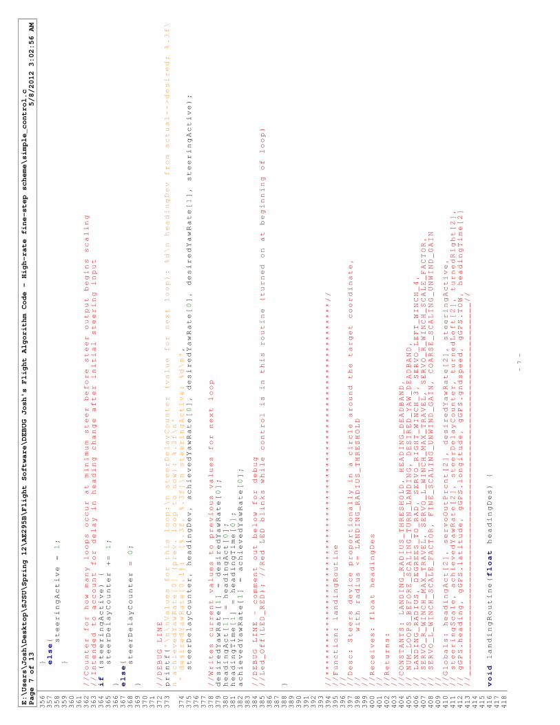
E:\Users\Josh\Desktop\SJSU\Spring 12\AE295B\Flight Software\DEBUG Josh's Flight Algorithm Code - High-rate fine-step scheme\simple_control.c
Page 7 of 13
5/8/2012 3:02:56 AM
356
}357
else{
358
steeringActive = 1;
359
}360
361
362
//Counter for how many loops occur at minimum steer before steer output begins scaling
363
//Intended to account for delay in heading change after initial steering input
364
if (steeringActive) {
365
steerDelayCounter += 1;
366
}367
else{
368
steerDelayCounter = 0;
369
}370
371
372
//DEBUG LINE
373
printf("\n\nValues for this loop:\n steerDelayCounter (value for next loop): %d\n headingDev from actual-->desired: %.3f\
n achievedYawRate[0] (prev. loop to now): %.3f\n"
374
" desiredYawRate[0,1]: [%.3f, %.3f]\n steeringActive: %d\n",
375
steerDelayCounter, headingDev, achievedYawRate[0], desiredYawRate[0], desiredYawRate[1], steeringActive);
376
377
378
//Writes current values to previous values for next loop
379
desiredYawRate[1] = desiredYawRate[0];
380
headingAct[1] = headingAct[0];
381
headingTime[1] = headingTime[0];
382
achievedYawRate[1] = achievedYawRate[0];
383
384
//DEBUG LINE - comment out below for debug
385
//Led_Off(LED_RED); //Red LED blinks while control is in this routine (turned on at beginning of loop)
386
387
388
}
389
390
391
392
393
394
//********************************************************************//
395
//Function: landingRoutine
396
//
397
//Desc: Steers device proportionally in a circle around the target coordinate,
398
//
with radius <= LANDING_RADIUS_THRESHOLD
399
//
400
//Receives: float headingDes
401
//
402
//Returns:
403
//
404
//CONSTANTS: LANDING_RADIUS_THRESHOLD, HEADING_DEADBAND,
405
// NUM_LOOPS_BEFORE_SCALING_TURN_LANDING, DESIRED_YAW_DEADBAND,
406
// LANDING_RADIUS, DEGREES_TO_RAD, SERVO_RIGHT_WINCH_3, SERVO_LEFT_WINCH_4,
407
// SERVO_R_WINCH_MAX_TRAVEL, SERVO_L_WINCH_MAX_TRAVEL, SERVO_R_WINCH_SCALE_FACTOR,
408
// SERVO_L_WINCH_SCALE_FACTOR, FINE_SCALING_UNWIND_GAIN, COARSE_SCALING_UNWIND_GAIN
409
//
410
//Globals: headingAct[2], servoOutPrcnt[2], desiredYawRate[2], steeringActive,
411
// steeringScale, achievedYawRate[2], steerDelayCounter, turnedLeft[2], turnedRight[2],
412
// gGPS.heading, gGPS.latitude, gGPS.longitude, gGPS.gndspeed, gGPS.TOW, headingTime[2]
413
//____________________________________________________________________//
414
415
416
void landingRoutine(float headingDes) {
417
418
- 7 -
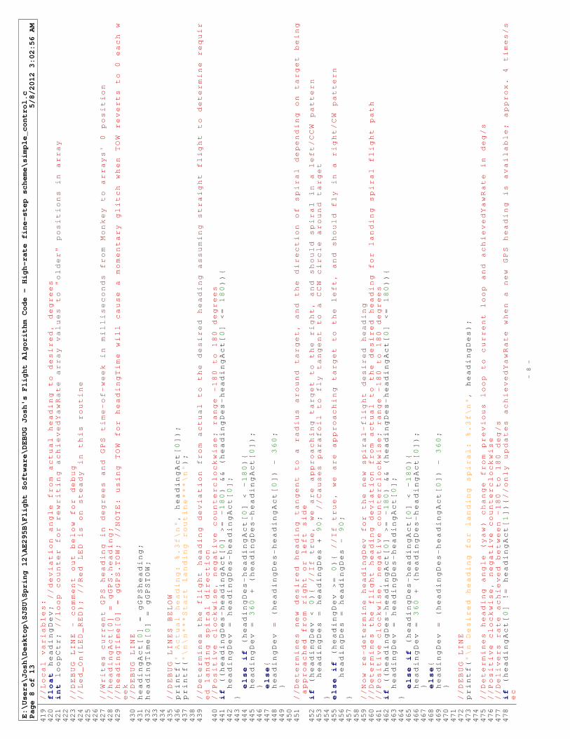
E:\Users\Josh\Desktop\SJSU\Spring 12\AE295B\Flight Software\DEBUG Josh's Flight Algorithm Code - High-rate fine-step scheme\simple_control.c
Page 8 of 13
5/8/2012 3:02:56 AM
419
//Local variables:
420
float headingDev; //deviation angle from actual heading to desired, degrees
421
int loopCtr; //loop counter for rewriting achievedYawRate array values to "older" positions in array
422
423
//DEBUG LINE - comment out below for debug
424
//Led_On(LED_RED); //Red LED is on steady in this routine
425
426
427
//Writes current GPS heading in degrees and GPS time-of-week in milliseconds from Monkey to arrays' 0 position
428
//headingAct[0] = gGPS.heading;
429
//headingTime[0] = gGPS.TOW; //NOTE: using TOW for headingTime will cause a momentary glitch when TOW reverts to 0 each w
eek
430
//DEBUG LINE
431
headingAct[0] = gGPSheading;
432
headingTime[0] = gGPSTOW;
433
434
435
//DEBUG LINES BELOW
436
printf(" Actual heading: %.3f\n", headingAct[0]);
437
printf("\n\n***Start landing routine***\n");
438
439
//Determines the flight heading deviation from actual to the desired heading assuming straight flight to determine requir
ed landing spiral direction
440
//Positive clockwise, negative counterclockwise; range -180 to 180 degrees
441
if ((headingDes-headingAct[0] >= -180) && (headingDes-headingAct[0] <= 180)){
442
headingDev = headingDes-headingAct[0];
443
}444
else if (headingDes-headingAct[0] < -180){
445
headingDev = 360 + (headingDes-headingAct[0]);
446
}
447
else{
448
headingDev = (headingDes-headingAct[0]) - 360;
449
}
450
451
//Determines new desired heading tangent to a radius around target, and the direction of spiral depending on target being
approached from right or left side
452
if (headingDev < 0){ //If true, we are approaching target to the right, and should spiral in a left/CCW pattern
453
headingDes = headingDes + 90; //Causes parafoil to fly tangent to a CCW circle around target
454
}455
else if (headingDev >= 0){ //If true, we are approaching target to the left, and should fly in a right/CW pattern
456
headingDes = headingDes - 90;
457
}458
459
//Now re-determine headingDev for the new spiral-flight desired heading
460
//Determines the flight heading deviation from actual to the desired heading for landing spiral flight path
461
//Positive clockwise, negative counterclockwise; range -180 to 180 degrees
462
if ((headingDes-headingAct[0] >= -180) && (headingDes-headingAct[0] <= 180)){
463
headingDev = headingDes-headingAct[0];
464
}465
else if (headingDes-headingAct[0] < -180){
466
headingDev = 360 + (headingDes-headingAct[0]);
467
}
468
else{
469
headingDev = (headingDes-headingAct[0]) - 360;
470
}
471
472
//DEBUG LINE
473
printf("\n Desired heading for landing spiral: %.3f\n", headingDes);
474
475
//Determines heading angle (yaw) change from previous loop to current loop and achievedYawRate in deg/s
476
//Positive clockwise, negative counterclockwise
477
//Delivers rate achieved between -180 to 180 deg/s
478
if (headingAct[0] != headingAct[1]){//only updates achievedYawRate when a new GPS heading is available; approx. 4 times/s
ec
- 8 -
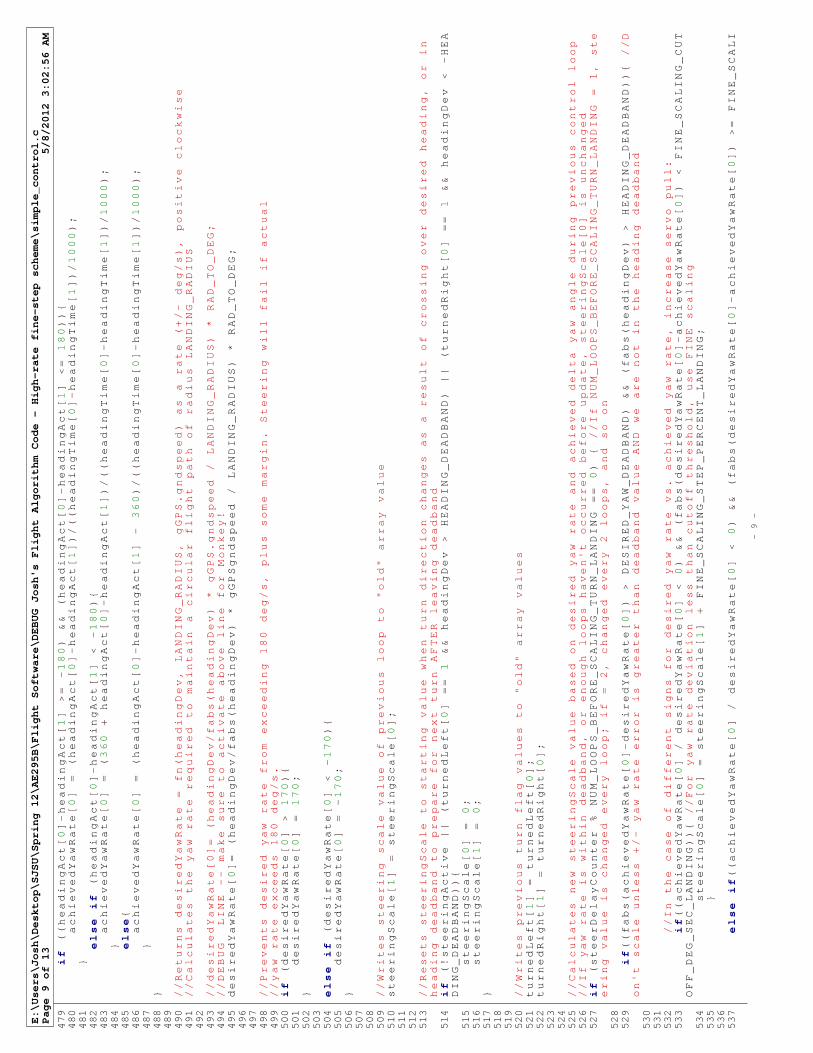
E:\Users\Josh\Desktop\SJSU\Spring 12\AE295B\Flight Software\DEBUG Josh's Flight Algorithm Code - High-rate fine-step scheme\simple_control.c
Page 9 of 13
5/8/2012 3:02:56 AM
479
if ((headingAct[0]-headingAct[1] >= -180) && (headingAct[0]-headingAct[1] <= 180)){
480
achievedYawRate[0] = (headingAct[0]-headingAct[1])/((headingTime[0]-headingTime[1])/1000);
481
}482
else if (headingAct[0]-headingAct[1] < -180){
483
achievedYawRate[0] = (360 + headingAct[0]-headingAct[1])/((headingTime[0]-headingTime[1])/1000);
484
}
485
else{
486
achievedYawRate[0] = (headingAct[0]-headingAct[1] - 360)/((headingTime[0]-headingTime[1])/1000);
487
}
488
}489
490
//Returns desiredYawRate = fn(headingDev, LANDING_RADIUS, gGPS.gndspeed) as a rate (+/- deg/s), positive clockwise
491
//Calculates the yaw rate required to maintain a circular flight path of radius LANDING_RADIUS
492
493
//desiredYawRate[0]= (headingDev/fabs(headingDev) * gGPS.gndspeed / LANDING_RADIUS) * RAD_TO_DEG;
494
//DEBUG LINE -- make sure to activate above line for Monkey!
495
desiredYawRate[0]= (headingDev/fabs(headingDev) * gGPSgndspeed / LANDING_RADIUS) * RAD_TO_DEG;
496
497
498
//Prevents desired yaw rate from exceeding 180 deg/s, plus some margin. Steering will fail if actual
499
//yaw rate exceeds 180 deg/s.
500
if (desiredYawRate[0] > 170){
501
desiredYawRate[0] = 170;
502
}503
504
else if (desiredYawRate[0] < -170){
505
desiredYawRate[0] = -170;
506
}507
508
509
//Writes steering scale value of previous loop to "old" array value
510
steeringScale[1] = steeringScale[0];
511
512
513
//Resets steeringScale to starting value when turn direction changes as a result of crossing over desired heading, or in
heading deadband to prepare for next turn AFTER leaving deadband
514
if (!steeringActive || (turnedLeft[0] == 1 && headingDev > HEADING_DEADBAND) || (turnedRight[0] == 1 && headingDev < -HEA
DING_DEADBAND)){
515
steeringScale[0] = 0;
516
steeringScale[1] = 0;
517
}518
519
520
//Writes previous turn flag values to "old" array values
521
turnedLeft[1] = turnedLeft[0];
522
turnedRight[1] = turnedRight[0];
523
524
525
//Calculates new steeringScale value based on desired yaw rate and achieved delta yaw angle during previous control loop
526
//If yaw rate is within deadband, or enough loops haven't occurred before update, steeringScale[0] is unchanged
527
if (steerDelayCounter % NUM_LOOPS_BEFORE_SCALING_TURN_LANDING == 0) { //If NUM_LOOPS_BEFORE_SCALING_TURN_LANDING = 1, ste
ering value is changed every loop; if = 2, changed every 2 loops, and so on
528
529
if((fabs(achievedYawRate[0]-desiredYawRate[0]) > DESIRED_YAW_DEADBAND) && (fabs(headingDev) > HEADING_DEADBAND)){ //D
on't scale unless +/- yaw rate error is greater than deadband value AND we are not in the heading deadband
530
531
532
//In the case of different signs for desired yaw rate vs. achieved yaw rate, increase servo pull:
533
if((achievedYawRate[0] / desiredYawRate[0] < 0) && (fabs(desiredYawRate[0]-achievedYawRate[0]) < FINE_SCALING_CUT
OFF_DEG_SEC_LANDING)){ //For yaw rate deviation less than cutoff threshold, use FINE scaling
534
steeringScale[0] = steeringScale[1] + FINE_SCALING_STEP_PERCENT_LANDING;
535
}536
537
else if((achievedYawRate[0] / desiredYawRate[0] < 0) && (fabs(desiredYawRate[0]-achievedYawRate[0]) >= FINE_SCALI
- 9 -
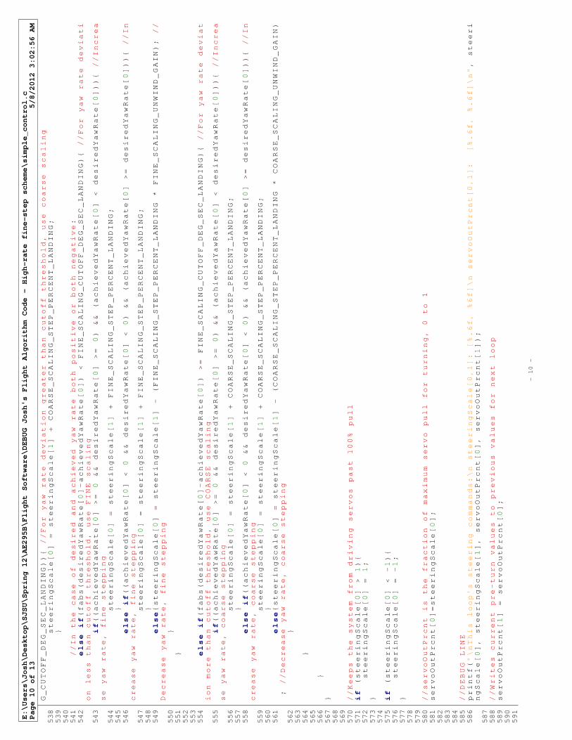
E:\Users\Josh\Desktop\SJSU\Spring 12\AE295B\Flight Software\DEBUG Josh's Flight Algorithm Code - High-rate fine-step scheme\simple_control.c
Page 10 of 13
5/8/2012 3:02:56 AM
G_CUTOFF_DEG_SEC_LANDING)){ //For yaw rate deviation greater than cutoff threshold, use coarse scaling
538
steeringScale[0] = steeringScale[1] + COARSE_SCALING_STEP_PERCENT_LANDING;
539
}540
541
//In the case of desired and achieved yaw rate both positive or both negative:
542
else if(fabs(desiredYawRate[0]-achievedYawRate[0]) < FINE_SCALING_CUTOFF_DEG_SEC_LANDING){ //For yaw rate deviati
on less than cutoff threshold, use FINE scaling
543
if((achievedYawRate[0] >= 0 && desiredYawRate[0] >= 0) && (achievedYawRate[0] < desiredYawRate[0])){ //Increa
se yaw rate, fine stepping
544
steeringScale[0] = steeringScale[1] + FINE_SCALING_STEP_PERCENT_LANDING;
545
}546
else if((achievedYawRate[0] < 0 && desiredYawRate[0] < 0) && (achievedYawRate[0] >= desiredYawRate[0])){ //In
crease yaw rate, fine stepping
547
steeringScale[0] = steeringScale[1] + FINE_SCALING_STEP_PERCENT_LANDING;
548
}549
else{steeringScale[0] = steeringScale[1] - (FINE_SCALING_STEP_PERCENT_LANDING * FINE_SCALING_UNWIND_GAIN); //
Decrease yaw rate, fine stepping
550
}551
}552
553
554
else if(fabs(desiredYawRate[0]-achievedYawRate[0]) >= FINE_SCALING_CUTOFF_DEG_SEC_LANDING){ //For yaw rate deviat
ion more than cutoff threshold, use COARSE scaling
555
if((achievedYawRate[0] >= 0 && desiredYawRate[0] >= 0) && (achievedYawRate[0] < desiredYawRate[0])){ //Increa
se yaw rate, coarse stepping
556
steeringScale[0] = steeringScale[1] + COARSE_SCALING_STEP_PERCENT_LANDING;
557
}558
else if((achievedYawRate[0] < 0 && desiredYawRate[0] < 0) && (achievedYawRate[0] >= desiredYawRate[0])){ //In
crease yaw rate, coarse stepping
559
steeringScale[0] = steeringScale[1] + COARSE_SCALING_STEP_PERCENT_LANDING;
560
}561
else{steeringScale[0] = steeringScale[1] - (COARSE_SCALING_STEP_PERCENT_LANDING * COARSE_SCALING_UNWIND_GAIN)
; //Decrease yaw rate, coarse stepping
562
}
563
564
}
565
566
}567
}568
569
570
//Keeps the system from driving servos past 100% pull
571
if (steeringScale[0] > 1){
572
steeringScale[0] = 1;
573
}574
575
if (steeringScale[0] < -1){
576
steeringScale[0] = -1;
577
}578
579
580
//servoOutPrcnt is the fraction of maximum servo pull for turning, 0 to 1
581
servoOutPrcnt[0]=steeringScale[0];
582
583
584
585
//DEBUG LINE
586
printf("\nThis loop's steering commands:\n steeringScale[0,1]: [%.6f, %6f]\n servoOutPrcnt[0,1]: [%.6f, %.6f]\n", steeri
ngScale[0], steeringScale[1], servoOutPrcnt[0], servoOutPrcnt[1]);
587
588
//Writes current pre-turn values to previous values for next loop
589
servoOutPrcnt[1] = servoOutPrcnt[0];
590
591
- 10 -
E:\Users\Josh\Desktop\SJSU\Spring 12\AE295B\Flight Software\DEBUG Josh's Flight Algorithm Code - High-rate fine-step scheme\simple_control.c
Page 11 of 13
5/8/2012 3:02:56 AM
592
//Determines which direction to turn and commands the servos to steer, scaled by steeringScale
593
//If steeringScale=1, full deflection is commanded (5.75 inch toggle line pull on parafoil)
594
if ((headingDev < -HEADING_DEADBAND && servoOutPrcnt[0] >= 0) || (headingDev > HEADING_DEADBAND && servoOutPrcnt[0] < 0
)) //then turn left!
595
{
596
servo_out[ SERVO_LEFT_WINCH_4 ].value = servo_out[ SERVO_LEFT_WINCH_4 ].value_failsafe -
597
(fabs(servoOutPrcnt[0])*SERVO_L_WINCH_MAX_TRAVEL*SERVO_L_WINCH_SCALE_FACTOR);
598
599
servo_out[ SERVO_RIGHT_WINCH_3 ].value = servo_out[ SERVO_RIGHT_WINCH_3 ].value_failsafe;
600
//For DEBUG, disable next line
601
//Servos_Update_All();
602
603
if (headingDev < -HEADING_DEADBAND && servoOutPrcnt[0] >= 0){//flag set for left turn, but ONLY for a turn not cause
d by negative servo value
604
turnedLeft[0] = 1;
605
turnedRight[0] = 0;
606
}
607
608
//DEBUG LINE BELOW
609
printf("\nSteering Left\n");
610
}
611
else if ((headingDev > HEADING_DEADBAND && servoOutPrcnt[0] >= 0) || (headingDev < -HEADING_DEADBAND && servoOutPrcnt[0
] < 0)) //then turn right!
612
{
613
servo_out[ SERVO_RIGHT_WINCH_3 ].value = servo_out[ SERVO_RIGHT_WINCH_3 ].value_failsafe +
614
(fabs(servoOutPrcnt[0])*SERVO_R_WINCH_MAX_TRAVEL*SERVO_R_WINCH_SCALE_FACTOR);
615
616
servo_out[ SERVO_LEFT_WINCH_4 ].value = servo_out[ SERVO_LEFT_WINCH_4 ].value_failsafe;
617
//For DEBUG, disable next line
618
//Servos_Update_All();
619
620
if (headingDev > HEADING_DEADBAND && servoOutPrcnt[0] >= 0){//flag set for left turn, but ONLY for a turn not caused
by negative servo value
621
turnedRight[0] = 1;
622
turnedLeft[0] = 0;
623
}
624
625
//DEBUG LINE BELOW
626
printf("\nSteering Right\n");
627
}
628
else
629
{ turnedLeft[0] = 0;
630
turnedRight[0] = 0;
631
632
//DEBUG LINE BELOW
633
printf("\nServos Unchanged -- In Heading Deadband\n");
634
}
635
636
637
638
//Sets steeringActive flag true if steering occurred earlier this loop and
639
//disables the reset of steering scale to 1 until straight flight resumes
640
if (headingDev > -HEADING_DEADBAND && headingDev < HEADING_DEADBAND) {
641
steeringActive = 0;
642
}643
else{
644
steeringActive = 1;
645
}646
647
648
//Counter for how many loops occur at minimum steer before steer output begins scaling
649
//Intended to account for delay in heading change after initial steering input
650
if (steeringActive) {
651
steerDelayCounter += 1;
- 11 -
E:\Users\Josh\Desktop\SJSU\Spring 12\AE295B\Flight Software\DEBUG Josh's Flight Algorithm Code - High-rate fine-step scheme\simple_control.c
Page 12 of 13
5/8/2012 3:02:56 AM
652
}653
else{
654
steerDelayCounter = 0;
655
}656
657
658
//DEBUG LINE
659
printf("\n\nValues for this loop:\n steerDelayCounter (value for next loop): %d\n headingDev from actual-->desired: %.3f\
n achievedYawRate[0] (prev. loop to now): %.3f\n"
660
" desiredYawRate[0,1]: [%.3f, %.3f]\n steeringActive: %d\n",
661
steerDelayCounter, headingDev, achievedYawRate[0], desiredYawRate[0], desiredYawRate[1], steeringActive);
662
663
664
//Writes current values to previous values for next loop
665
desiredYawRate[1] = desiredYawRate[0];
666
headingAct[1] = headingAct[0];
667
headingTime[1] = headingTime[0];
668
achievedYawRate[1] = achievedYawRate[0];
669
670
671
}672
673
674
675
676
//********************************************************************//
677
//Function: landingFlare
678
//
679
//Desc: Performs a simple flare maneuver when parafoil system altitude
680
//
is less than FLARE_HEIGHT above ground
681
//
682
//Receives:
683
//
684
//Returns:
685
//
686
//CONSTANTS: SERVO_RIGHT_WINCH_3, SERVO_LEFT_WINCH_4, SERVO_R_WINCH_MAX_TRAVEL,
687
// SERVO_L_WINCH_MAX_TRAVEL, SERVO_R_WINCH_SCALE_FACTOR,
688
// SERVO_L_WINCH_SCALE_FACTOR, FLARE_PRCNT
689
//
690
//Globals:
691
//____________________________________________________________________//
692
693
694
void landingFlare(void) {
695
696
//Sets both servos to a percentage of maximum pull to perform braking flare near landing
697
servo_out[ SERVO_RIGHT_WINCH_3 ].value = servo_out[ SERVO_RIGHT_WINCH_3 ].value_failsafe +
698
(FLARE_PRCNT*SERVO_R_WINCH_MAX_TRAVEL*SERVO_R_WINCH_SCALE_FACTOR);
699
700
servo_out[ SERVO_LEFT_WINCH_4 ].value = servo_out[ SERVO_LEFT_WINCH_4 ].value_failsafe -
701
(FLARE_PRCNT*SERVO_L_WINCH_MAX_TRAVEL*SERVO_L_WINCH_SCALE_FACTOR);
702
703
//For DEBUG, disable next line
704
//Servos_Update_All();
705
706
//DEBUG LINE
707
printf("\n\n***Initiate landing flare***\n Left Servo Value: %.3f\n Right Servo Value: %.3f\n", FLARE_PRCNT, FLARE_PR
CNT);
708
709
710
}711
712
713
//End Josh's control code
- 12 -
E:\Users\Josh\Desktop\SJSU\Spring 12\AE295B\Flight Software\DEBUG Josh's Flight Algorithm Code - High-rate fine-step scheme\simple_control.c
Page 13 of 13
5/8/2012 3:02:56 AM
714
//_______________________________________________________________________________________________________________________
_____________________________________________________________________
715
//***********************************************************************************************************************
*********************************************************************
716
- 13 -

132
Appendix B
Addendum - High Altitude Balloon Flight Results, May 19, 2012
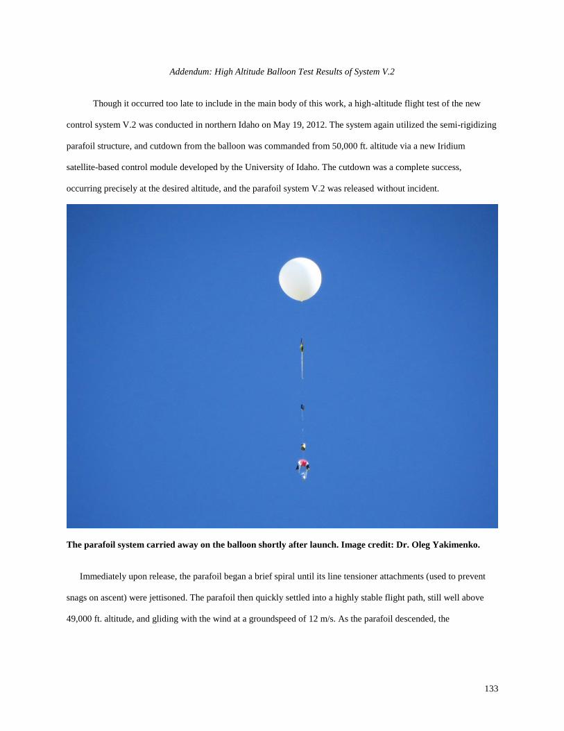
133
Addendum: High Altitude Balloon Test Results of System V.2
Though it occurred too late to include in the main body of this work, a high-altitude flight test of the new
control system V.2 was conducted in northern Idaho on May 19, 2012. The system again utilized the semi-rigidizing
parafoil structure, and cutdown from the balloon was commanded from 50,000 ft. altitude via a new Iridium
satellite-based control module developed by the University of Idaho. The cutdown was a complete success,
occurring precisely at the desired altitude, and the parafoil system V.2 was released without incident.
The parafoil system carried away on the balloon shortly after launch. Image credit: Dr. Oleg Yakimenko.
Immediately upon release, the parafoil began a brief spiral until its line tensioner attachments (used to prevent
snags on ascent) were jettisoned. The parafoil then quickly settled into a highly stable flight path, still well above
49,000 ft. altitude, and gliding with the wind at a groundspeed of 12 m/s. As the parafoil descended, the
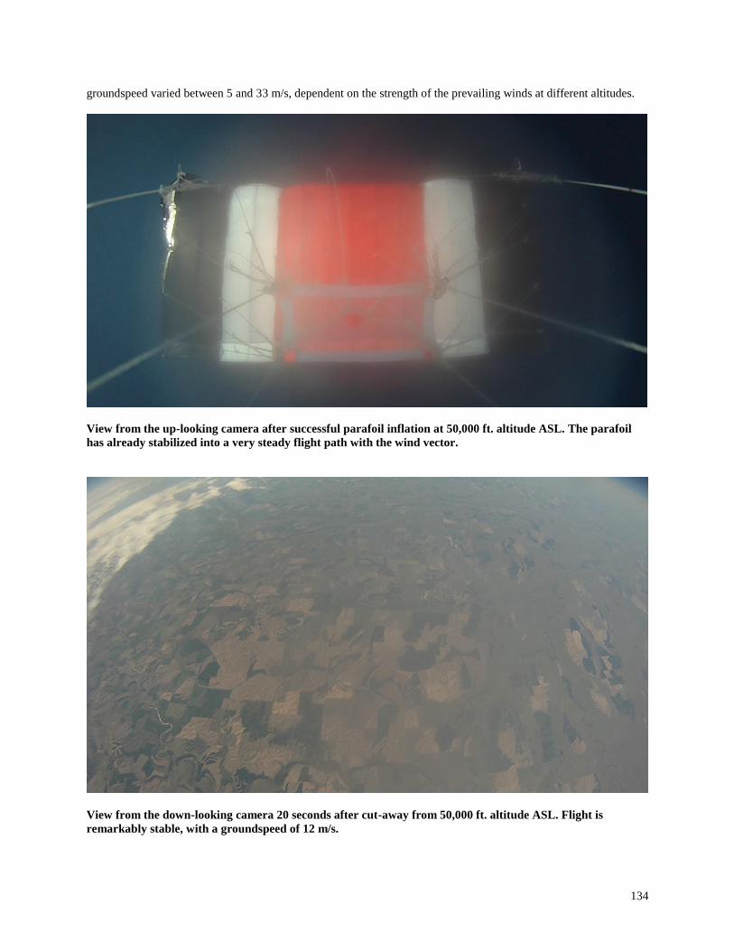
134
groundspeed varied between 5 and 33 m/s, dependent on the strength of the prevailing winds at different altitudes.
View from the up-looking camera after successful parafoil inflation at 50,000 ft. altitude ASL. The parafoil
has already stabilized into a very steady flight path with the wind vector.
View from the down-looking camera 20 seconds after cut-away from 50,000 ft. altitude ASL. Flight is
remarkably stable, with a groundspeed of 12 m/s.
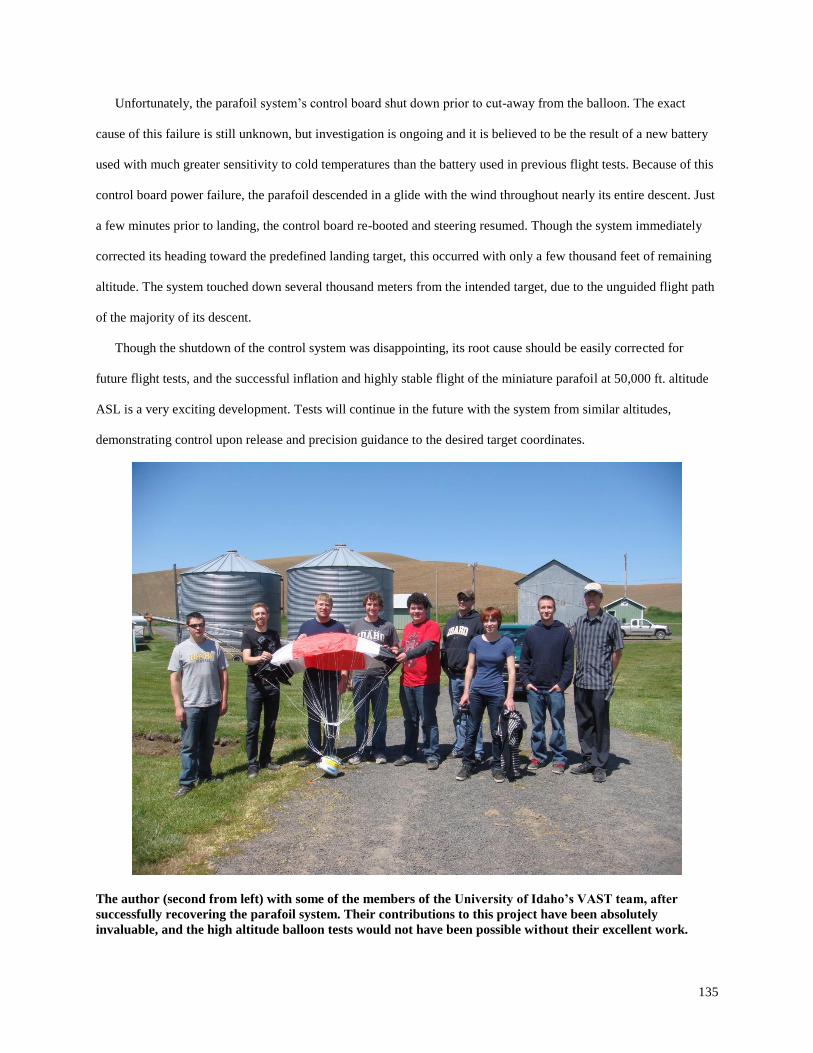
135
Unfortunately, the parafoil system’s control board shut down prior to cut-away from the balloon. The exact
cause of this failure is still unknown, but investigation is ongoing and it is believed to be the result of a new battery
used with much greater sensitivity to cold temperatures than the battery used in previous flight tests. Because of this
control board power failure, the parafoil descended in a glide with the wind throughout nearly its entire descent. Just
a few minutes prior to landing, the control board re-booted and steering resumed. Though the system immediately
corrected its heading toward the predefined landing target, this occurred with only a few thousand feet of remaining
altitude. The system touched down several thousand meters from the intended target, due to the unguided flight path
of the majority of its descent.
Though the shutdown of the control system was disappointing, its root cause should be easily corrected for
future flight tests, and the successful inflation and highly stable flight of the miniature parafoil at 50,000 ft. altitude
ASL is a very exciting development. Tests will continue in the future with the system from similar altitudes,
demonstrating control upon release and precision guidance to the desired target coordinates.
The author (second from left) with some of the members of the University of Idaho’s VAST team, after
successfully recovering the parafoil system. Their contributions to this project have been absolutely
invaluable, and the high altitude balloon tests would not have been possible without their excellent work.
Recommended