
Mini-project report
Computational Fluid Dynamics
Analysis of a Low Cost Wind Turbine
Jon Leary – [email protected]
June 2010
Abstract
Computational Fluid Dynamics (CFD) software was used to compare the performance of a hand-
made wind turbine blade with that of a conventional factory made model. The geometry was
simplified to 2D aerofoils and the surrounding flow field was analysed at a Reynold’s number of
80,000. It was found that the lift/drag characteristics of the two aerofoils across a range of angles of
attack were virtually identical, meaning that the torque force exerted on the wind turbine blades
would also be identical and therefore as would the power outputs of the two turbines. However, the
simple model ignored a number of important issues, such as 3D effects and the influence of
manufacturing quality on the idealised blade geometry. Further modelling and/or experimental
validation work is needed to increase confidence in the quality of the results.
Table of Contents
Abstract ............................................................................................................................................ 2
1 Introduction to Small Scale Wind Power .................................................................................... 3
2 Aims and Objectives .................................................................................................................. 3
3 Basic Aerodynamic Theory of Horizontal Axis Wind Turbines (HAWTs) ....................................... 4
3.1 The Aerofoil ....................................................................................................................... 4
3.2 Lift and Drag, Thrust and Torque ........................................................................................ 5
3.3 Reynold’s Number .............................................................................................................. 8
3.4 Boundary Layers................................................................................................................. 9
3.5 Stall .................................................................................................................................... 9
3.6 Aerofoil Geometry ........................................................................................................... 10
4 Introduction to Computational Fluid Dynamics (CFD) ............................................................... 11
4.1 The Modelling Process ..................................................................................................... 11
4.2 CFD for Wind Turbine Analysis ......................................................................................... 12
5 Building the Model .................................................................................................................. 12
5.1 Modelling Software .......................................................................................................... 12
5.2 Modelling Strategy ........................................................................................................... 12
5.3 Aerofoil Geometry ........................................................................................................... 13
5.3.1 2D Modelling Domain ............................................................................................... 13
5.3.2 Turbulence Model .................................................................................................... 14
6 Results ..................................................................................................................................... 16
7 Analysis ................................................................................................................................... 18
8 Evaluation................................................................................................................................ 18
9 Conclusion ............................................................................................................................... 18
10 References ........................................................................................................................... 19
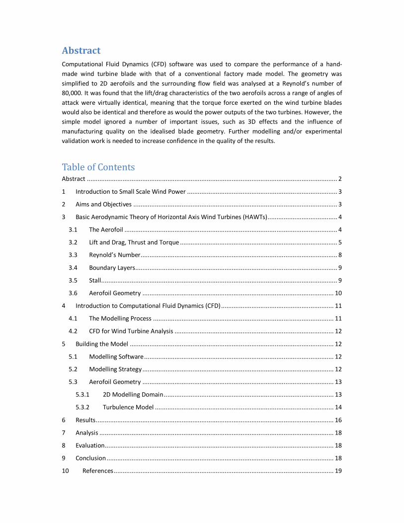
1 Introduction to Small Scale Wind Power
Small scale wind turbines can be used to provide power
to remote areas of the developing world that are far
away from any existing electrical grid system. The
electricity they supply can be used to provide light in the
mornings and evenings which can allow children to
study and further their opportunities in later life or
adults to continue working and provide that little bit of
extra income for their families that could allow them to
work their way out of poverty. Unfortunately, at a cost
of thousands of pounds, factory built small scale wind
turbines are expensive, even for reasonably well off
citizens of the developed world. Families in the
developing world living below the poverty line often
have to survive on less than $US 1 (~70p) [3] per day,
keeping these potentially revolutionary machines way
out of their reach. However, it is possible to build small
scale wind turbines by hand, using basic workshop tools
and techniques. Designs for such machines are freely
available as open source documents on the internet to
give people in the developing world access to the
technology. Machines such as Hugh Piggott’s [2]
Horizontal Axis Wind Turbine (HAWT) shown in Figure 1 have been tried and tested throughout the
developed and developing world and have proved an invaluable aid to the remote communities in
which they have been installed. At around £500, they cost a fraction of their factory made
counterparts and consequently bring wind power within the reach of isolated small community
groups in the developing world.
2 Aims and Objectives
Piggott’s design may be tried and tested, but has it been truly optimised? Obviously a compromise
has been struck between performance, cost, durability and manufacturability, but is there a way to
improve the performance of the machine without significantly affecting the other factors? This
project aims to:
• Compare the performance of Piggott’s wooden hand carved wind turbine blades with those
of a conventional factory made turbine.
• Propose and evaluate appropriate techniques for improving the efficiency of Piggott’s
turbine blades.
Figure 1 - 1kW wind turbine installed in
Tanzania [2]
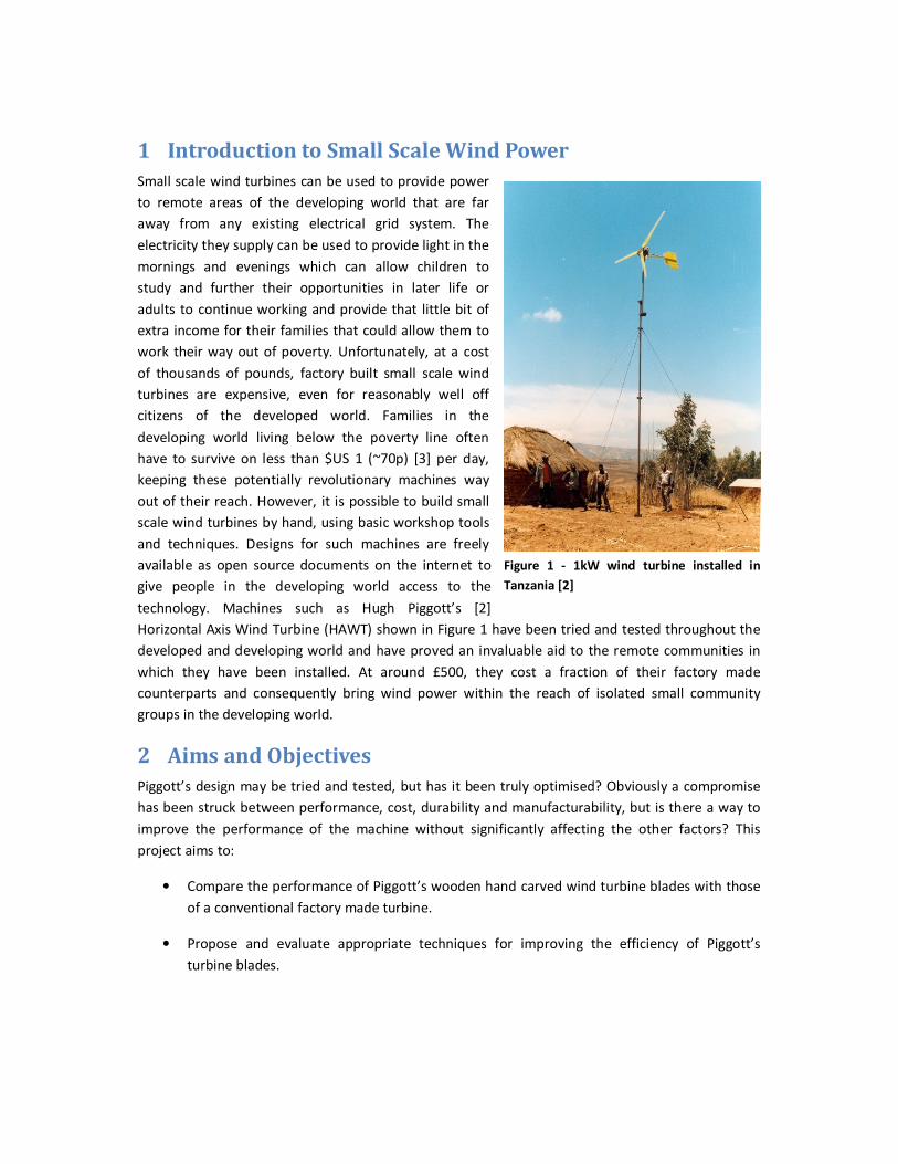
3 Basic Aerodynamic Theory of Horizontal Axis Wind
Turbines (HAWTs)
Lift-based Horizontal Axis Wind
Turbines (HAWTs) have today
become the standard
mechanism for harnessing the
power in the wind and
converting it into electricity.
They evolved from the grain
grinding drag-based windmills
of yesteryear. As aeronautics
took off during the last century
with the commercialisation of
aeroplane technology, more
and more became known about
wing technology. The three-
bladed wind turbines we see all
around us today evolved from
aircraft wing theory and are
essentially three wings bolted
onto a generator with a
common central axis. They use
lift from the oncoming wind to
rotate themselves about this
central axis, which points
horizontally into the wind,
hence the name HAWT. Vertical
Axis Wind Turbines (VAWTs)
are also used, but the higher
efficiencies of HAWTs have made them the dominant technology in today’s society.
3.1 The Aerofoil
An aerofoil (or airfoil in the USA) is a 2D shape capable of producing a reactive lift force when in
motion relative to the surrounding air. Most commonly known as the cross-sectional profile of an
aircraft’s wing, Figure 2 shows how the 3D geometry of a lift-based HAWT blade also consists of a
series of aerofoil profiles. Figure 3 gives an overview of the basic aerofoil terminology.
LIF
T
DRAG
Figure 2 - 2D Aerofoil section through a 3D lift-based HAWT blade
(Adapted from [1])
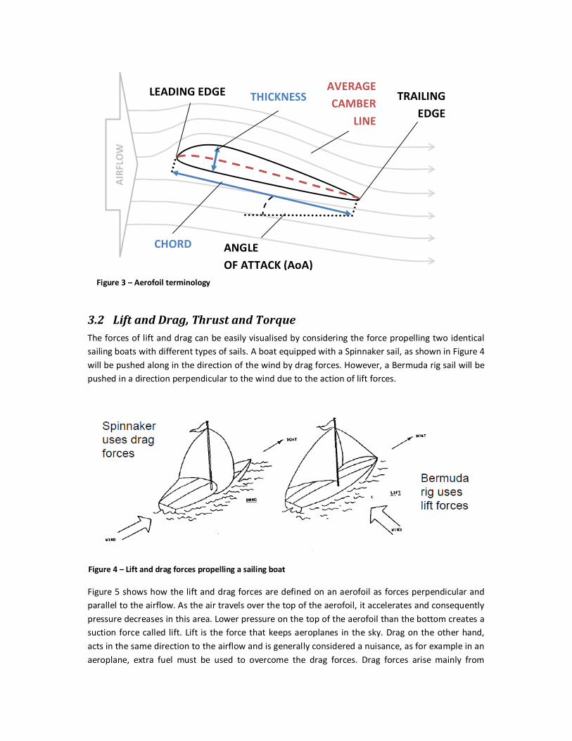
3.2 Lift and Drag, Thrust and Torque
The forces of lift and drag can be easily visualised by considering the force propelling two identical
sailing boats with different types of sails. A boat equipped with a Spinnaker sail, as shown in Figure 4
will be pushed along in the direction of the wind by drag forces. However, a Bermuda rig sail will be
pushed in a direction perpendicular to the wind due to the action of lift forces.
Figure 5 shows how the lift and drag forces are defined on an aerofoil as forces perpendicular and
parallel to the airflow. As the air travels over the top of the aerofoil, it accelerates and consequently
pressure decreases in this area. Lower pressure on the top of the aerofoil than the bottom creates a
suction force called lift. Lift is the force that keeps aeroplanes in the sky. Drag on the other hand,
acts in the same direction to the airflow and is generally considered a nuisance, as for example in an
aeroplane, extra fuel must be used to overcome the drag forces. Drag forces arise mainly from
AIR
FLO
W
LEADING EDGE AVERAGE
CAMBER
LINE
CHORD
TRAILING
EDGE
THICKNESS
ANGLE
OF ATTACK (AoA)
Figure 3 – Aerofoil terminology
Figure 4 – Lift and drag forces propelling a sailing boat
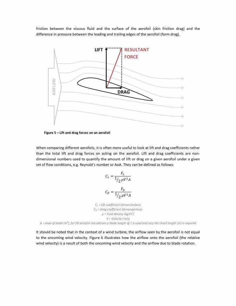
friction between the viscous fluid and the surface of the aerofoil (skin friction drag) and the
difference in pressure between the leading and trailing edges of the aerofoil (form drag).
When comparing different aerofoils, it is often more useful to look at lift and drag coefficients rather
than the total lift and drag forces on acting on the aerofoil. Lift and drag coefficients are non-
dimensional numbers used to quantify the amount of lift or drag on a given aerofoil under a given
set of flow conditions, e.g. Reynold’s number or AoA. They can be defined as follows:
�� ���
12� ��
�� ���
12� ��
CL = Lift coefficient (dimensionless)
CD = Drag coefficient (dimensionless)
ρ = Fluid density (kg/m3)
V = Velocity (m/s)
A = Area of blade (m2), for 2D aerofoil calculations a blade length of 1 is used and only the chord length (m) is required
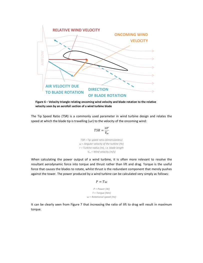
It should be noted that in the context of a wind turbine, the airflow seen by the aerofoil is not equal
to the oncoming wind velocity. Figure 6 illustrates how the airflow onto the aerofoil (the relative
wind velocity) is a result of both the oncoming wind velocity and the airflow due to blade rotation.
LIFT
DRAG
RESULTANT
FORCE A
IRF
LOW
Figure 5 – Lift and drag forces on an aerofoil
The Tip Speed Ratio (TSR) is a commonly used parameter in wind turbine design and relates the
speed at which the blade tip is travelling (ωr) to the velocity of the oncoming wind:
�� ���
�
TSR = Tip speed ratio (dimensionless)
ω = Angular velocity of the turbine (Hz)
r = Turbine radius (m), i.e. blade length
V∞ = Wind velocity (m/s)
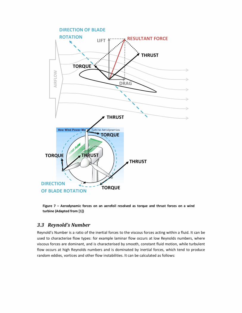
When calculating the power output of a wind turbine, it is often more relevant to resolve the
resultant aerodynamic force into torque and thrust rather than lift and drag. Torque is the useful
force that causes the blades to rotate, whilst thrust is the redundant component that merely pushes
against the tower. The power produced by a wind turbine can be calculated very simply as follows:
� � �
P = Power (W)
T = Torque (Nm)
ω = Rotational speed (Hz)
It can be clearly seen from Figure 7 that increasing the ratio of lift to drag will result in maximum
torque.
ONCOMING WIND
VELOCITY
DIRECTION
OF BLADE ROTATION
RELATIVE WIND VELOCITY
AIR
FLO
W
AIR VELOCITY DUE
TO BLADE ROTATION
Figure 6 – Velocity triangle relating oncoming wind velocity and blade rotation to the relative
velocity seen by an aerofoil section of a wind turbine blade
3.3 Reynold’s Number
Reynold’s Number is a ratio of the inertial forces to the viscous forces acting within a fluid. It can be
used to characterise flow types: for example laminar flow occurs at low Reynolds numbers, where
viscous forces are dominant, and is characterised by smooth, constant fluid motion, while turbulent
flow occurs at high Reynolds numbers and is dominated by inertial forces, which tend to produce
random eddies, vortices and other flow instabilities. It can be calculated as follows:
LIFT
DRAG
RESULTANT FORCE
AIR
FLO
W
THRUST
TORQUE
THRUST
TORQUE
THRUST
TORQUE
TORQUE THRUST
Figure 7 – Aerodynamic forces on an aerofoil resolved as torque and thrust forces on a wind
turbine (Adapted from [1])
DIRECTION
OF BLADE ROTATION
DIRECTION OF BLADE
ROTATION
�� ��������� ������
������ ��������
! ��
!
Re = Reynold’s number (dimensionless)
ρ = Fluid density (kg/m3)
V = Fluid velocity (m/s)
L = Characteristic length (m), e.g. aerofoil chord length
µ = Dynamic viscosity (kg/ms)
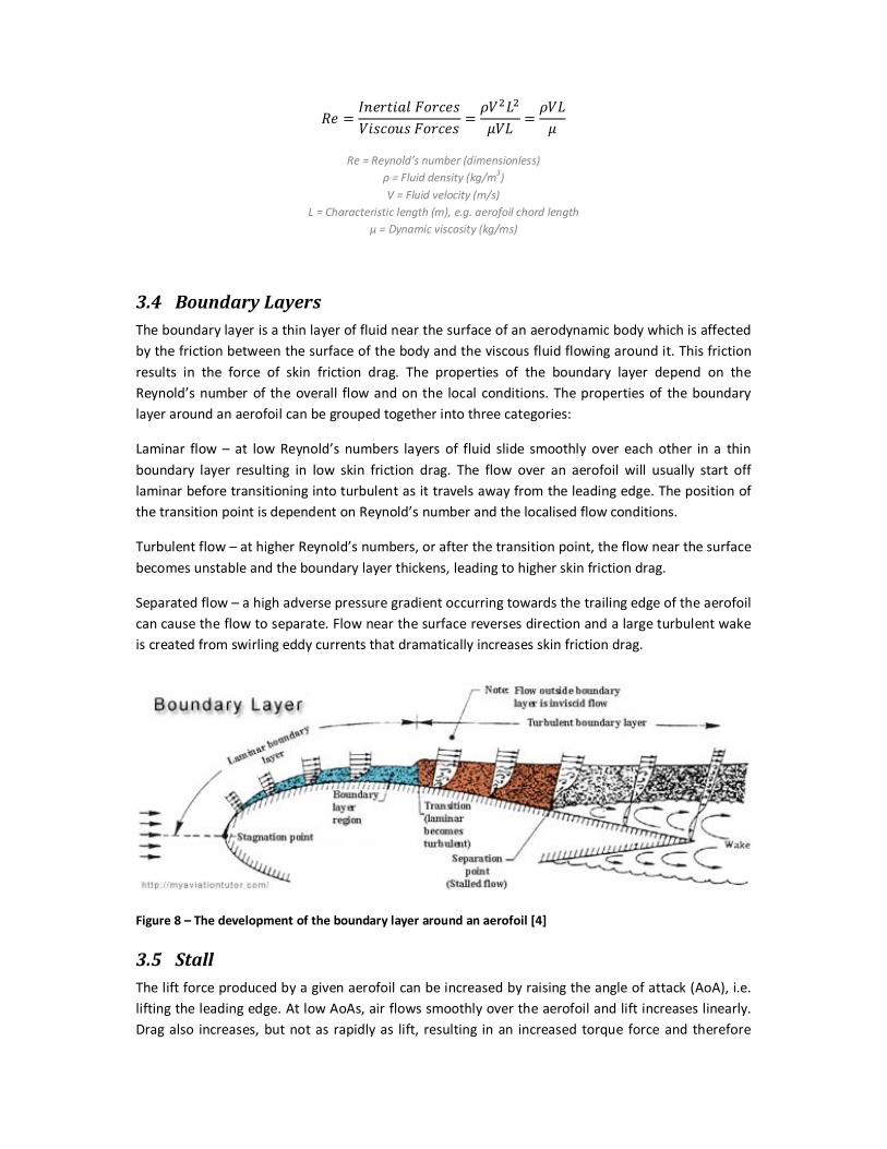
3.4 Boundary Layers
The boundary layer is a thin layer of fluid near the surface of an aerodynamic body which is affected
by the friction between the surface of the body and the viscous fluid flowing around it. This friction
results in the force of skin friction drag. The properties of the boundary layer depend on the
Reynold’s number of the overall flow and on the local conditions. The properties of the boundary
layer around an aerofoil can be grouped together into three categories:
Laminar flow – at low Reynold’s numbers layers of fluid slide smoothly over each other in a thin
boundary layer resulting in low skin friction drag. The flow over an aerofoil will usually start off
laminar before transitioning into turbulent as it travels away from the leading edge. The position of
the transition point is dependent on Reynold’s number and the localised flow conditions.
Turbulent flow – at higher Reynold’s numbers, or after the transition point, the flow near the surface
becomes unstable and the boundary layer thickens, leading to higher skin friction drag.
Separated flow – a high adverse pressure gradient occurring towards the trailing edge of the aerofoil
can cause the flow to separate. Flow near the surface reverses direction and a large turbulent wake
is created from swirling eddy currents that dramatically increases skin friction drag.
Figure 8 – The development of the boundary layer around an aerofoil [4]
3.5 Stall
The lift force produced by a given aerofoil can be increased by raising the angle of attack (AoA), i.e.
lifting the leading edge. At low AoAs, air flows smoothly over the aerofoil and lift increases linearly.
Drag also increases, but not as rapidly as lift, resulting in an increased torque force and therefore
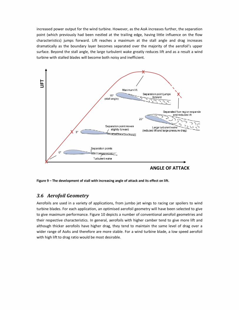
increased power output for the wind turbine. However, as the AoA increases further, the separation
point (which previously had been nestled at the trailing edge, having little influence on the flow
characteristics) jumps forward. Lift reaches a maximum at the stall angle and drag increases
dramatically as the boundary layer becomes separated over the majority of the aerofoil’s upper
surface. Beyond the stall angle, the large turbulent wake greatly reduces lift and as a result a wind
turbine with stalled blades will become both noisy and inefficient.
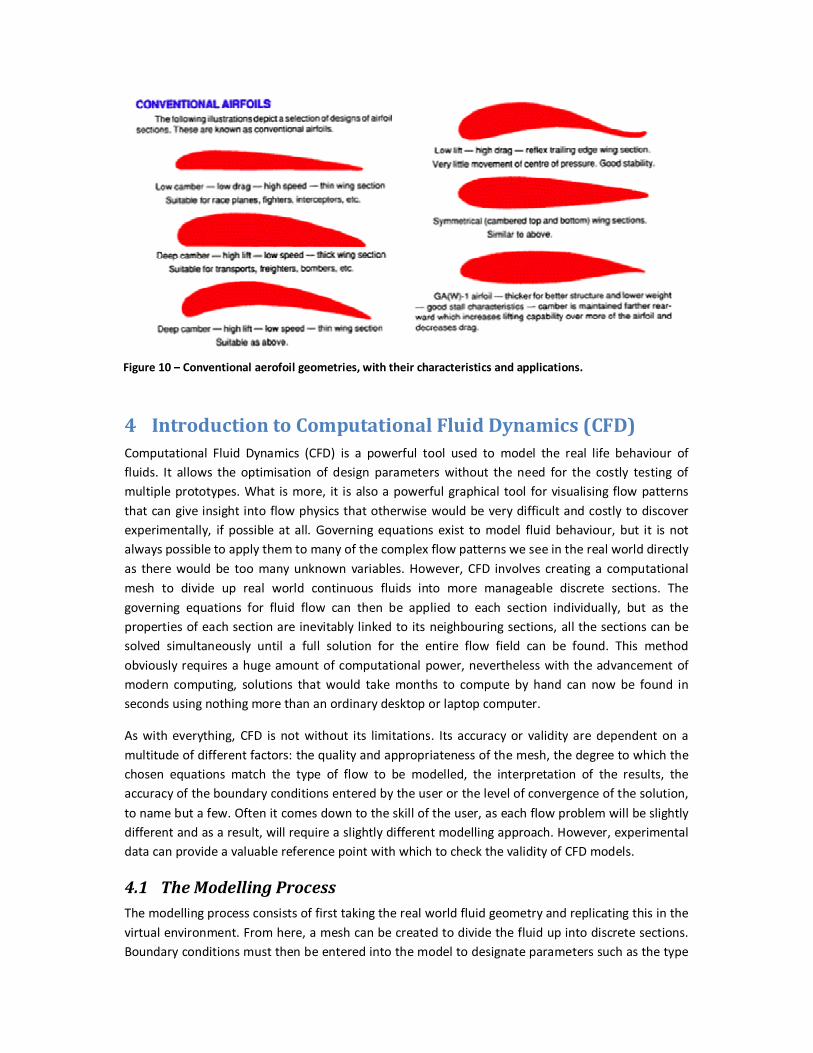
3.6 Aerofoil Geometry
Aerofoils are used in a variety of applications, from jumbo jet wings to racing car spoilers to wind
turbine blades. For each application, an optimised aerofoil geometry will have been selected to give
to give maximum performance. Figure 10 depicts a number of conventional aerofoil geometries and
their respective characteristics. In general, aerofoils with higher camber tend to give more lift and
although thicker aerofoils have higher drag, they tend to maintain the same level of drag over a
wider range of AoAs and therefore are more stable. For a wind turbine blade, a low speed aerofoil
with high lift to drag ratio would be most desirable.
ANGLE OF ATTACK
X
X
X
X
Figure 9 – The development of stall with increasing angle of attack and its effect on lift.
LIF
T
4 Introduction to Computational Fluid Dynamics (CFD)
Computational Fluid Dynamics (CFD) is a powerful tool used to model the real life behaviour of
fluids. It allows the optimisation of design parameters without the need for the costly testing of
multiple prototypes. What is more, it is also a powerful graphical tool for visualising flow patterns
that can give insight into flow physics that otherwise would be very difficult and costly to discover
experimentally, if possible at all. Governing equations exist to model fluid behaviour, but it is not
always possible to apply them to many of the complex flow patterns we see in the real world directly
as there would be too many unknown variables. However, CFD involves creating a computational
mesh to divide up real world continuous fluids into more manageable discrete sections. The
governing equations for fluid flow can then be applied to each section individually, but as the
properties of each section are inevitably linked to its neighbouring sections, all the sections can be
solved simultaneously until a full solution for the entire flow field can be found. This method
obviously requires a huge amount of computational power, nevertheless with the advancement of
modern computing, solutions that would take months to compute by hand can now be found in
seconds using nothing more than an ordinary desktop or laptop computer.
As with everything, CFD is not without its limitations. Its accuracy or validity are dependent on a
multitude of different factors: the quality and appropriateness of the mesh, the degree to which the
chosen equations match the type of flow to be modelled, the interpretation of the results, the
accuracy of the boundary conditions entered by the user or the level of convergence of the solution,
to name but a few. Often it comes down to the skill of the user, as each flow problem will be slightly
different and as a result, will require a slightly different modelling approach. However, experimental
data can provide a valuable reference point with which to check the validity of CFD models.
4.1 The Modelling Process
The modelling process consists of first taking the real world fluid geometry and replicating this in the
virtual environment. From here, a mesh can be created to divide the fluid up into discrete sections.
Boundary conditions must then be entered into the model to designate parameters such as the type
Figure 10 – Conventional aerofoil geometries, with their characteristics and applications.
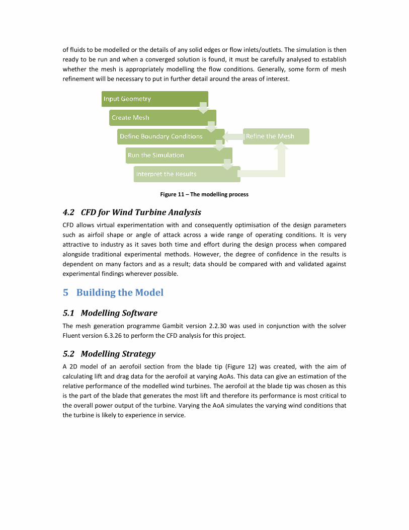
of fluids to be modelled or the details of any solid edges or flow inlets/outlets. The simulation is then
ready to be run and when a converged solution is found, it must be carefully analysed to establish
whether the mesh is appropriately modelling the flow conditions. Generally, some form of mesh
refinement will be necessary to put in further detail around the areas of interest.
Figure 11 – The modelling process
4.2 CFD for Wind Turbine Analysis
CFD allows virtual experimentation with and consequently optimisation of the design parameters
such as airfoil shape or angle of attack across a wide range of operating conditions. It is very
attractive to industry as it saves both time and effort during the design process when compared
alongside traditional experimental methods. However, the degree of confidence in the results is
dependent on many factors and as a result; data should be compared with and validated against
experimental findings wherever possible.
5 Building the Model
5.1 Modelling Software
The mesh generation programme Gambit version 2.2.30 was used in conjunction with the solver
Fluent version 6.3.26 to perform the CFD analysis for this project.
5.2 Modelling Strategy
A 2D model of an aerofoil section from the blade tip (Figure 12) was created, with the aim of
calculating lift and drag data for the aerofoil at varying AoAs. This data can give an estimation of the
relative performance of the modelled wind turbines. The aerofoil at the blade tip was chosen as this
is the part of the blade that generates the most lift and therefore its performance is most critical to
the overall power output of the turbine. Varying the AoA simulates the varying wind conditions that
the turbine is likely to experience in service.
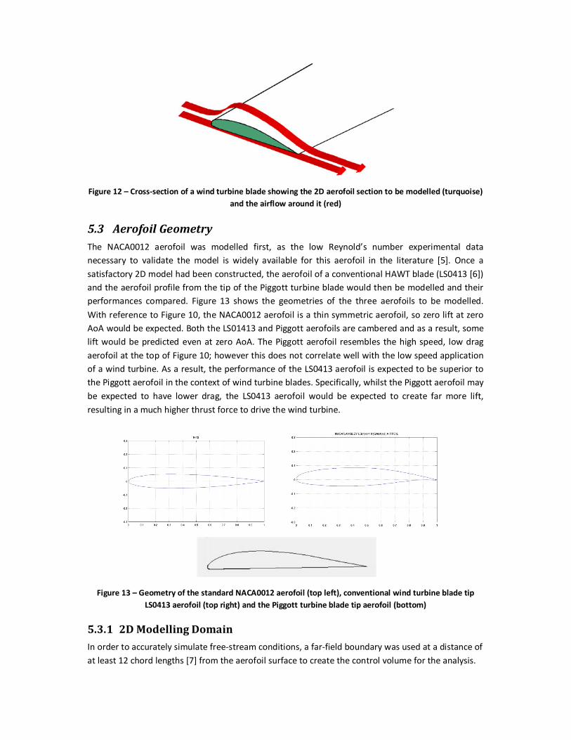
Figure 12 – Cross-section of a wind turbine blade showing the 2D aerofoil section to be modelled (turquoise)
and the airflow around it (red)
5.3 Aerofoil Geometry
The NACA0012 aerofoil was modelled first, as the low Reynold’s number experimental data
necessary to validate the model is widely available for this aerofoil in the literature [5]. Once a
satisfactory 2D model had been constructed, the aerofoil of a conventional HAWT blade (LS0413 [6])
and the aerofoil profile from the tip of the Piggott turbine blade would then be modelled and their
performances compared. Figure 13 shows the geometries of the three aerofoils to be modelled.
With reference to Figure 10, the NACA0012 aerofoil is a thin symmetric aerofoil, so zero lift at zero
AoA would be expected. Both the LS01413 and Piggott aerofoils are cambered and as a result, some
lift would be predicted even at zero AoA. The Piggott aerofoil resembles the high speed, low drag
aerofoil at the top of Figure 10; however this does not correlate well with the low speed application
of a wind turbine. As a result, the performance of the LS0413 aerofoil is expected to be superior to
the Piggott aerofoil in the context of wind turbine blades. Specifically, whilst the Piggott aerofoil may
be expected to have lower drag, the LS0413 aerofoil would be expected to create far more lift,
resulting in a much higher thrust force to drive the wind turbine.
Figure 13 – Geometry of the standard NACA0012 aerofoil (top left), conventional wind turbine blade tip
LS0413 aerofoil (top right) and the Piggott turbine blade tip aerofoil (bottom)
5.3.1 2D Modelling Domain
In order to accurately simulate free-stream conditions, a far-field boundary was used at a distance of
at least 12 chord lengths [7] from the aerofoil surface to create the control volume for the analysis.
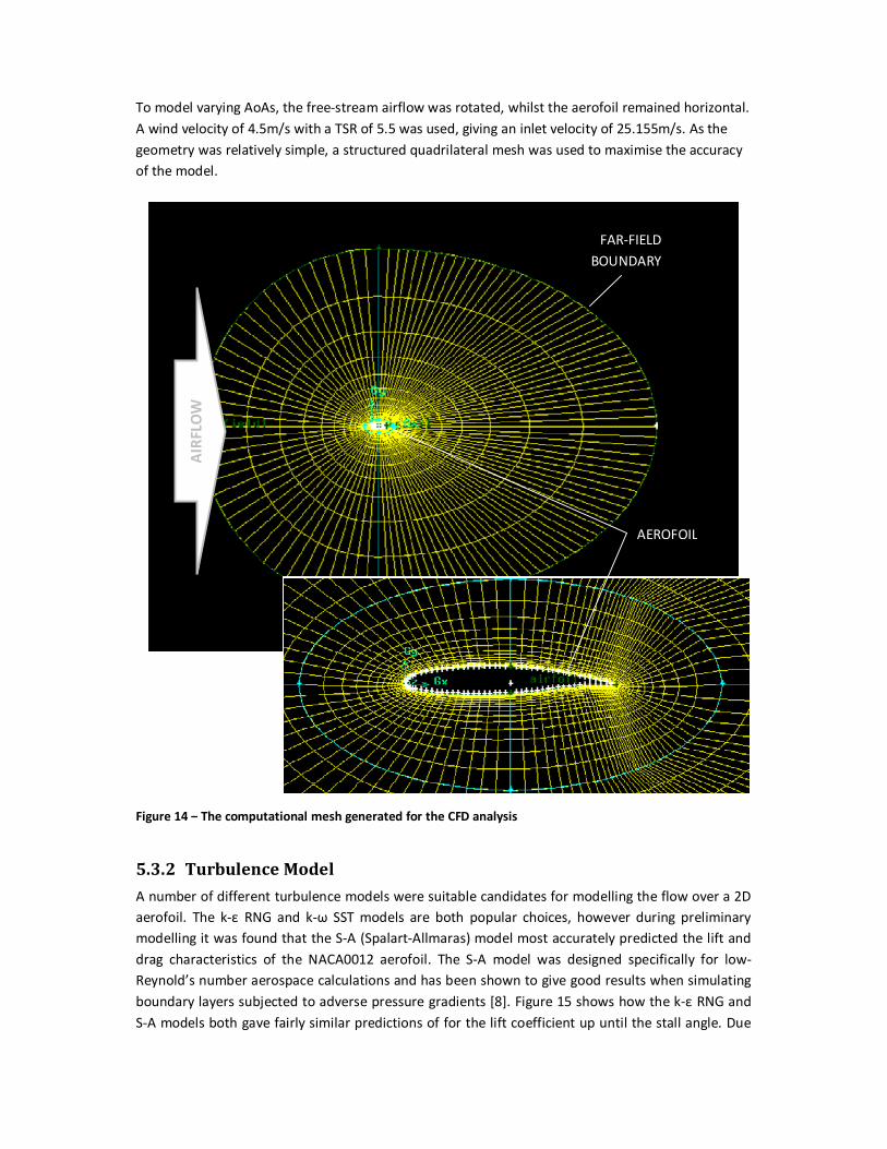
To model varying AoAs, the free-stream airflow was rotated, whilst the aerofoil remained horizontal.
A wind velocity of 4.5m/s with a TSR of 5.5 was used, giving an inlet velocity of 25.155m/s. As the
geometry was relatively simple, a structured quadrilateral mesh was used to maximise the accuracy
of the model.
5.3.2 Turbulence Model
A number of different turbulence models were suitable candidates for modelling the flow over a 2D
aerofoil. The k-ε RNG and k-ω SST models are both popular choices, however during preliminary
modelling it was found that the S-A (Spalart-Allmaras) model most accurately predicted the lift and
drag characteristics of the NACA0012 aerofoil. The S-A model was designed specifically for low-
Reynold’s number aerospace calculations and has been shown to give good results when simulating
boundary layers subjected to adverse pressure gradients [8]. Figure 15 shows how the k-ε RNG and
S-A models both gave fairly similar predictions of for the lift coefficient up until the stall angle. Due
FAR-FIELD
BOUNDARY
AEROFOIL
AIR
FLO
W
Figure 14 – The computational mesh generated for the CFD analysis

to the turbulent nature of the physical flow conditions that are being modelled close to and beyond
the stall angle, complex time-varying simulations would be required to correctly simulate this
behaviour. As a result, the data obtained from this simple steady-state model in this region cannot
be considered reliable. With regards to the drag coefficient, Figure 15 clearly demonstrates that the
S-A model gives a far better match to the experimental data. As a result, it was decided to use the S-
A turbulence model for the main analysis.
Figure 15 - Comparison of k-ε RNG and S-A turbulence models for the NACA0012 aerofoil for validation
against low Reynold’s number experimental data
0
0.1
0.2
0.3
0.4
0.5
0.6
0.7
0.8
0.9
1
0 5 10 15 20
Lift
Co
eff
icie
nt
Angle of Attack
NACA 0012 Model Validation Study
Lift Coefficient
Experimental, Re=160,000 k-E RNG, Re=80,000 S-A, Re=80,000
0
0.05
0.1
0.15
0.2
0.25
0.3
0.35
0 5 10 15 20 25
Dra
g C
oe
ffic
ien
t
Angle of Attack
NACA 0012 Model Validation Study
Drag Coefficient
k-E RNG, Re=80,000 Experimental, Re=160,000 S-A, Re=80,000
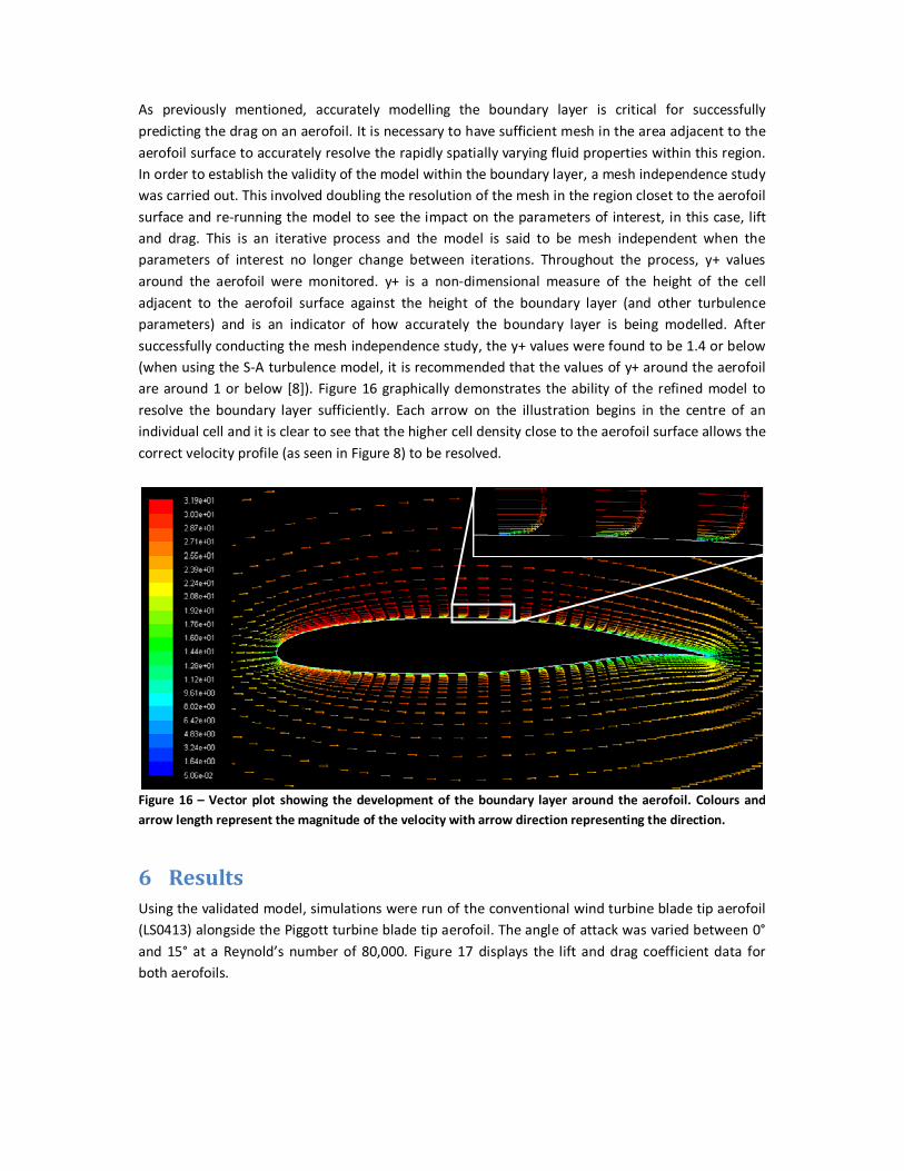
As previously mentioned, accurately modelling the boundary layer is critical for successfully
predicting the drag on an aerofoil. It is necessary to have sufficient mesh in the area adjacent to the
aerofoil surface to accurately resolve the rapidly spatially varying fluid properties within this region.
In order to establish the validity of the model within the boundary layer, a mesh independence study
was carried out. This involved doubling the resolution of the mesh in the region closet to the aerofoil
surface and re-running the model to see the impact on the parameters of interest, in this case, lift
and drag. This is an iterative process and the model is said to be mesh independent when the
parameters of interest no longer change between iterations. Throughout the process, y+ values
around the aerofoil were monitored. y+ is a non-dimensional measure of the height of the cell
adjacent to the aerofoil surface against the height of the boundary layer (and other turbulence
parameters) and is an indicator of how accurately the boundary layer is being modelled. After
successfully conducting the mesh independence study, the y+ values were found to be 1.4 or below
(when using the S-A turbulence model, it is recommended that the values of y+ around the aerofoil
are around 1 or below [8]). Figure 16 graphically demonstrates the ability of the refined model to
resolve the boundary layer sufficiently. Each arrow on the illustration begins in the centre of an
individual cell and it is clear to see that the higher cell density close to the aerofoil surface allows the
correct velocity profile (as seen in Figure 8) to be resolved.
6 Results
Using the validated model, simulations were run of the conventional wind turbine blade tip aerofoil
(LS0413) alongside the Piggott turbine blade tip aerofoil. The angle of attack was varied between 0°
and 15° at a Reynold’s number of 80,000. Figure 17 displays the lift and drag coefficient data for
both aerofoils.
Figure 16 – Vector plot showing the development of the boundary layer around the aerofoil. Colours and
arrow length represent the magnitude of the velocity with arrow direction representing the direction.
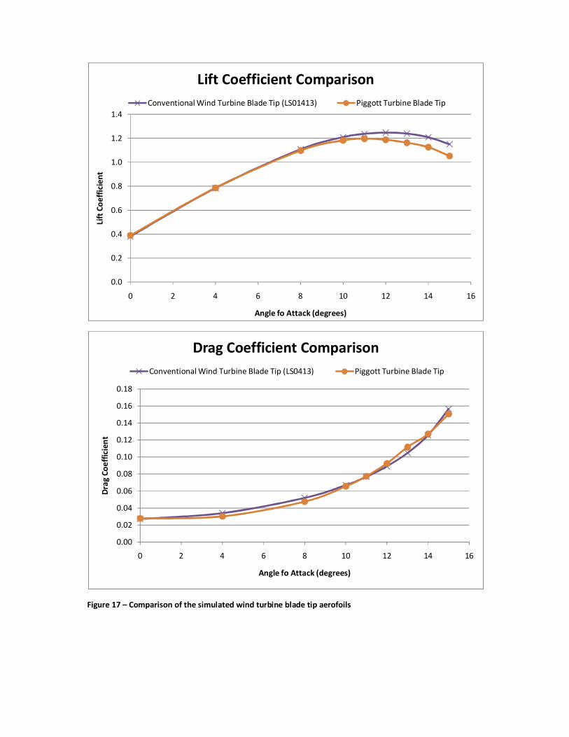
Figure 17 – Comparison of the simulated wind turbine blade tip aerofoils
0.0
0.2
0.4
0.6
0.8
1.0
1.2
1.4
0 2 4 6 8 10 12 14 16
Lift
Co
eff
icie
nt
Angle fo Attack (degrees)
Lift Coefficient Comparison
Conventional Wind Turbine Blade Tip (LS01413) Piggott Turbine Blade Tip
0.00
0.02
0.04
0.06
0.08
0.10
0.12
0.14
0.16
0.18
0 2 4 6 8 10 12 14 16
Dra
g C
oe
ffic
ien
t
Angle fo Attack (degrees)
Drag Coefficient Comparison
Conventional Wind Turbine Blade Tip (LS0413) Piggott Turbine Blade Tip
7 Analysis
Figure 17 clearly indicates that the performance of the two wind turbine blade tip aerofoils is
virtually identical. This result is highly unexpected as the geometries of the two aerofoils are very
different. This would seem to suggest that wind turbines using either of these profiles would
produce similar amounts of power. The Piggott aerofoil is a far simpler shape to manufacture, as the
lower surface is effectively a flat surface and therefore it is a far more appropriate design for low-
cost hand manufacturing as virtually no performance is sacrificed.
8 Evaluation
Although the Piggott aerofoil may seem to have an identical performance to the conventional
LS0413 aerofoil, the model used was very simple and a number of factors that will influence the
performance of a wind turbine blade in real life were not included, for example:
• 3D effects – Real wind turbine blades are both twisted and tapered and encounter
increasing relative wind speeds towards the tip due to the rotation of the blade. Vortices are
also created at the ends of the blades due to the difference in pressure between the upper
and lower surfaces of the aerofoil. In order to correctly model the geometry of a wind
turbine blade, a 3D model would need to be built.
• Transition point – The point along the surface of the aerofoil at which the flow transitions
from laminar to turbulent is of critical importance to determining the drag on the aerofoil.
To date, no computational techniques are capable of predicting the location of this point
and experimental measurements must be taken to determine its location. As a result, the
entire boundary layer was modelled as turbulent and the drag is likely to be an over-
prediction.
• Idealised geometry – The wind turbine blade tips were modelled as ideal aerofoil
geometries, however this would not be the case in the real world. In particular, a hand-made
wind turbine blade is likely to be full of defects arising from poor manufacturing technique,
especially at the tip where the size of the aerofoil relative to the size of the tools is smallest.
These defects, although they may seem small, could have a critical impact on the aerofoil’s
performance as they could trip the flow from laminar to turbulent and consequently
increase drag. The surface roughness of the wind turbine blades was also not modelled,
which could also similarly affect the drag.
• Accuracy of CFD – As shown by Figure 15, the model still has a significant degree of
inaccuracy, especially near and above the stall angle. Further modelling is required to
increase the accuracy of the model, in particular unsteady simulations to more accurately
determine performance around stall angle.
• Experimental validation – Although the model was validated using the NACA0012 aerofoil,
the flow physics may be slightly different around the two test aerofoils and as a result
experimental data for these would give more confidence in the results.
9 Conclusion
Hugh Piggott’s DIY wind turbine has been shown to have comparable performance to that of a
conventional wind turbine. In the simplified model of the aerofoils at the blade tips, both exhibited
virtually identical lift and drag characteristics, implying that the torque force exerted on the blades
and consequently the power produced by the turbine would also be identical. However, the simple
model neglects many important factors such as 3D effects, geometric variations deriving from
manufacturing defects and the location of the transition point. As a result, further modelling and/or
experimental work is required to give more confidence in the results of this study.
10 References
[1] How Stuff Works.com. Available: www.howstuffworks.com, Accessed 18th July 2010
[2] H. Piggott. (2010, Scoraig Wind. Available: www.scoraigwind.com
[3] A. Doig, "Off-grid Electricity for Developing Countries," IEEE Review, pp. 25-28, 1999.
[4] 16th July). My Aviation Tutor. Available: http://myaviationtutor.com
[5] R. E. a. K. Sheldahl, P. C., "Aerodynamic Characteristics of Seven Airfoil Sections Through 180
Degrees Angle of Attack for Use in Aerodynamic Analysis of Vertical Axis Wind Turbines,"
Sandia National Laborotories, Albuquerque, New Mexico, USA1981.
[6] K. Kishinami, et al., "Theoretical and Experimental Study on the Aerodynamic Characteristics
of a Horizontal Axis Wind Turbine," Elsevier, 2005.
[7] R. Bhaskaran. 1st July). Cornell Fluent Tutorials - Flow Over an Airfoil. Available:
http://courses.cit.cornell.edu/fluent/airfoil/index.htm
[8] Fluent_Inc. (2005). Fluent 6.3.26 User Manual.
Recommended