Measuring Multi-Joint Stiffness during SingleMovements: Numerical Validation of a Novel Time-Frequency ApproachDavide Piovesan1,2,3*, Alberto Pierobon3, Paul DiZio3,4, James R. Lackner3,4
1 Sensory Motor Performance Program, Rehabilitation Institute of Chicago, Chicago, Illinois, United States of America, 2 Department of Physical Medicine and
Rehabilitation, Northwestern University, Chicago, Illinois, United States of America, 3 Ashton Graybiel Spatial Orientation Laboratory, Brandeis University, Waltham,
Massachusetts, United States of America, 4 Volen Center for Complex Systems, Brandeis University, Waltham, Massachusetts, United States of America
Abstract
This study presents and validates a Time-Frequency technique for measuring 2-dimensional multijoint arm stiffnessthroughout a single planar movement as well as during static posture. It is proposed as an alternative to current regressivemethods which require numerous repetitions to obtain average stiffness on a small segment of the hand trajectory. Themethod is based on the analysis of the reassigned spectrogram of the arm’s response to impulsive perturbations and canestimate arm stiffness on a trial-by-trial basis. Analytic and empirical methods are first derived and tested through modalanalysis on synthetic data. The technique’s accuracy and robustness are assessed by modeling the estimation of stiffnesstime profiles changing at different rates and affected by different noise levels. Our method obtains results comparable withtwo well-known regressive techniques. We also test how the technique can identify the viscoelastic component of non-linear and higher than second order systems with a non-parametrical approach. The technique proposed here is veryimpervious to noise and can be used easily for both postural and movement tasks. Estimations of stiffness profiles arepossible with only one perturbation, making our method a useful tool for estimating limb stiffness during motor learningand adaptation tasks, and for understanding the modulation of stiffness in individuals with neurodegenerative diseases.
Citation: Piovesan D, Pierobon A, DiZio P, Lackner JR (2012) Measuring Multi-Joint Stiffness during Single Movements: Numerical Validation of a Novel Time-Frequency Approach. PLoS ONE 7(3): e33086. doi:10.1371/journal.pone.0033086
Editor: Paul L. Gribble, The University of Western Ontario, Canada
Received March 28, 2011; Accepted February 9, 2012; Published March 20, 2012
Copyright: � 2012 Piovesan et al. This is an open-access article distributed under the terms of the Creative Commons Attribution License, which permitsunrestricted use, distribution, and reproduction in any medium, provided the original author and source are credited.
Funding: This study was partially supported by NIH grants 2 R01AR048546-06 and 5 R01 MH086053-02 (www.nih.gov/).The funders had no role in study design,data collection and analysis, decision to publish, or preparation of the manuscript.
Competing Interests: The authors have declared that no competing interests exist.
* E-mail: [email protected]
Introduction
The motor system uses stiffness modulation to maintain stability
of the arm during interactions with the environment. It has been
experimentally investigated in both postural (i.e. static) and
dynamic paradigms. In limb postural experiments, system
identification is accomplished using either stochastic perturbations
[1,2,3,4,5] or regressive techniques [6,7,8,9,10]. Studies that
quantify stiffness as a function of hand position along a reaching
trajectory typically use regressive procedures [11,12,13,14,15,
16,17,18,19]. Stochastic methods are based on ensemble tech-
niques [20,21,22,23] and even though they identify the system
non-parametrically they require hundreds of perturbed repetitions
of the same movement to obtain a reliable estimate of stiffness.
These repetitions can induce muscle co-contraction that leads to
stiffening of the arm joints [24], and can strongly reduce stretch
reflexes [25]. Regressive techniques allow for more natural (not
continuously perturbed) movements, but still require many trials to
produce reasonable stiffness time-profiles using a parametric
approach. A method that could estimate dynamic changes in
arm stiffness on a trial-by-trial basis would constitute an ideal tool
to monitor changes in stiffness over time.
At present, the majority of regressive techniques to estimate
stiffness rely on the calculation of a baseline trajectory followed by
the application of a set of mechanical perturbations to the arm.
After several repeatable unperturbed trials, a prediction of the
unperturbed hand trajectory can be obtained with a time average
[14,15], a look-up table [11] or an auto-regressive (AR) model
[17,18,19]. Investigators have employed mechanical perturbations
of different types, such as force pulses [14,15], servo-displacements
[11,17], and virtual walls [16], that are generally applied by a
robotic manipulandum during randomly selected trials. When a
sufficient number of perturbations is delivered in multiple
directions at the same point along the arm kinematic profile,
stiffness is calculated by means of a regression between the
variation of hand kinematics and the forces generated by the
perturbation.
Regressive techniques rely on the assumption that unperturbed
arm movements are repeatable and that the mechanical
characteristics of the arm do not change over a small set of
repetitions (ergodicity), To obtain the estimation of the baseline
trajectory and a set of perturbation responses with such
techniques, a series of measures needs to be taken using the same
reproducible kinematic configuration; consequently, the data
collection burden can be substantial. If a servo-commanded
displacement is used, estimates of stiffness can be done
independently of the values of damping and inertia when the
perturbation reaches steady state [10,11,12,13,17,18,19,26]. As a
consequence, the required characteristics of the robotic devices
can be very demanding. In general, when using displacement
PLoS ONE | www.plosone.org 1 March 2012 | Volume 7 | Issue 3 | e33086
perturbations, a very stiff environment must be rendered by the
robot to keep the actual displacement of the hand as close as
possible to the perturbation imposed and to break the feedback
loop between joint torques and joint positions, effectively creating
an open-loop system that it is possible to identify [27].
The purpose of the present study is to present a technique for
measuring time-varying limb stiffness on a trial-by trial basis. The
technique is based on time-frequency domain and modal analysis.
It requires neither the assumption of stationarity nor the
repeatability of the motor task (ergodicity). To show the utility of
the proposed method we compare it with two well known
regressive techniques, one using force perturbations [15] and the
other displacement perturbations [7,8,11]. We demonstrate with
synthetic data that our proposed technique produces accurate
estimates of time-variant stiffness on a single trial basis, under both
static and dynamic conditions.
Time-frequency techniques are relatively new to the field of
motor control despite having been widely used in fields such as
structural engineering [28,29,30], radar, sonar, and medical
imaging [31]. They depend on evaluating the location of the
maximal energy density of a signal in the time-frequency domain.
We applied this approach to measure the response of a mechanical
system to a transient perturbation to identify the system features.
The versatility of this technique allows for several types of
perturbations to be used, including force impulses, hold and
release [32], and force steps. Classical regressive methods are
limited to estimating an average value of stiffness across several
trials; by contrast, our time-frequency technique can estimate the
variation of stiffness and damping across trials, thereby providing a
tool to study the relationship between stiffness modulation and
adaptive learning. The proposed method is non-parametric and
we tested it on higher-than-second-order and non-linear systems.
Modal analysis was used as a parameter identification method for
second-order systems to allow a direct comparison with regressive
techniques. Linearity, repeatability of the trajectory, and steady
state were not necessary assumptions, and a stiff robot was not
required because a free response was measured.
In the following sections, we outline how our method was
implemented and tested. First we describe the variational
approach we apply to the identification of a non-stationary
vibrating mechanical system. Then we explain how the system
identification is carried out in the time-frequency analysis by
means of a reassigned spectrogram, and how this tool allows a
parametric identification of time-varying second order mechanical
systems as well as a non-parametric identification of non-linear
and higher than second order systems (see ‘‘The spectrogram’’).
We provide a description of the models we used to simulate the
behavior of human arm movements, as well as a discussion of the
characteristics and limitation of each model (see ‘‘Assumptions and
possible relaxations’’). We then introduce and discuss the
assumptions under which our method operates, namely that the
system exhibits an oscillatory behavior, the instantaneous resonant
frequencies are separable, and the system’s stiffness and damping
matrices are symmetric, though no assumptions on the relation-
ship between stiffness and damping (e.g. proportional or classical
damping) are required.
We then show how the systems’ equations are normalized with
respect to the inertial matrix (see ‘‘Equation normalization’’), and
how the eigenvectors (see ‘‘identification of eigenvectors’’) and the
stiffness and damping parameters (see ‘‘system decoupling and
modal analysis’’) of a second order, two degree-of-freedom (DOF)
system are computed through the implementation of our modal
analysis.
We provide all the model parameters used in our simulations
(see ‘‘Description of the simulation’’), including the inertial
characteristics, the trajectory followed by the simulated arm, the
imposed stiffness and damping profiles that we identified, and the
parameters specific to each type of mechanical model. We also
provide the characteristics of the perturbations used in our
identification method, as well as the parameters used in our
implementation of previously proposed regressive techniques, to
which our method is compared.
Results of the simulations are then presented. The stiffness and
damping parameters identified with our method are shown to be
statistically comparable to those identified with regressive
techniques. Results of the non-parametrical system identification,
that our method allows, are also presented.
Methods
In this section, we provide a variational description of the
mechanical system response that is then used in our time-
frequency analysis. When studying the motion of a mechanical
system,~xx tð Þ is a vector of generalized position coordinates (angles,
Cartesian coordinates, etc.). We can define Dnx as the set
representing the position coordinates and their derivatives with
respect to time up to the nth order so that
Dnx~Lnx
Ltn,:::,
L2x
Lt2,L1x
Lt1,x
!, in general n[Q [33].
A mechanical system must comply with the Lagrange–
d’Alembert principle so that
M x,tð Þ d2
dt2~xx tð Þð Þz~ss Dnx,tð Þ~~gg Dnx,tð Þ ð1Þ
where M x,tð Þ is the inertial matrix of the system in the chosen
coordinate frame, ~gg Dnx,tð Þ is the external force field, and
~ss Dnx,tð Þ is the internal force field generated by the mechanical
network [33]. The goal is to identify the features of the unknown
internal force field ~ss Dnx,tð Þ.Since ~ss Dnx,tð Þ is generally a non-linear function of the
coordinates ~xx tð Þ and their derivatives, system identification is
difficult due to a lack of coherent and well defined theory for
appraising such computations. When the upper limb dynamics is
described, we expect the solution of equation (1) to be limited,
non-chaotic and quasi-periodic. With these premises, the non-
linear system (1) can be approximated with a time-varying locally
linear system and can be recast in the following polynomial form
[34]:
M x,tð Þ d2
dt2~xx tð Þð ÞzR Dn,tð Þx tð Þ~~gg Dnx,tð Þ ð2Þ
where:
R Dn,tð Þ~an tð Þ Ln
Ltnz:::za2 tð Þ L2
Lt2za1 tð Þ L1
Lt1za0 tð Þ, n[Q ð3Þ
is a polynomial operator[35].
Equation (2) is a model for a time-variant linear system whose
oscillating solutions can be found both in the time and frequency
domains by means of classical control theory. Assuming the system
is stationary (i.e. R Dnð Þ does not depend upon time and its
coefficients ak are constant), and under-damped, the measured
angular frequencies vj tð Þ in response to a perturbation of the
mechanical system (called resonant angular frequencies) are
Time-Frequency Approach to Measure Limb Stiffness
PLoS ONE | www.plosone.org 2 March 2012 | Volume 7 | Issue 3 | e33086
constant. Thus, classical Laplace transform techniques can be used
to approach the problem in the frequency domain where equation
(2) is recast in the form:
Ms2~XX sð Þz~SS sð Þ~~GG sð Þ ð4Þ
The resonant frequencies are represented by the peaks on the
absolute value of the complex spectrum of the solution of (4). If the
system is second order, modal analysis of vibrating systems offers a
variety of techniques to identify the characteristics of~ss Dnxð Þ from
the values of the constant resonant frequencies vj . Specifically,
coefficients ak of R Dnð Þx tð Þ can be identified. When the system is
linear but not stationary (i.e. the coefficients ak tð Þ are a function of
time), the frequency response following an impulsive perturbation
will vary as a function of time. In this condition, equation (4)
cannot track the time varying resonant frequencies and a new
approach must be taken to identify R Dn,tð Þx tð Þ. We achieved this
by adopting the variation of the joint angle dh?
tð Þ as the
independent coordinate for our analysis. The solutions of equation
(2) for the ith degree of freedom can then be expressed in terms of
instantaneous amplitude and phase [29]:
dhi tð Þ~Xn
j~1
Aji tð Þ:cos(Qj tð Þ): ð5Þ
where, Aji tð Þ is the instantaneous amplitude for the jth resonant
frequency associated with the ith degree of freedom and Qj is the
instantaneous phase. The jth instantaneous resonant (or damped)
angular frequency of the system is defined as the derivative with
respect to time of the jth instantaneous phase:
vj tð Þ~ _QQj tð Þð6Þ
We present a technique to measure vectors of instantaneous
resonant angular frequencies v! tð Þ and instantaneous amplitude
A!
i tð Þ, for the time-varying dynamics of a two degree-of-freedom
double-pendulum system during the free response to an impulsive
perturbation. The system models the human upper limb, during
either postural or reaching tasks. When v! tð Þ and A!
i tð Þ are
known, and the system is second order and locally linear, modal
analysis can be applied at each instant to reconstruct the
characteristics of the internal force field ~ss d Dnhð Þ,tð Þ~R Dn,tð Þx tð Þ.
The SpectrogramThe convolution of window function h(t) sliding along the non-
stationary time-variant signal dhi tð Þ as a function of time shift t is
called a ‘‘Short Term Fourier Transform’’ (STFT) and can be
expressed as:
STFT(v,t)~
ðz?
{?
dhi tð Þ:h(t{t)exp({jvt)dt ð7Þ
A spectrogram is the representation of a STFT calculated on
the signal dhi tð Þ for multiple time shifts t and is the tool used in
the implementation of our time-frequency analysis. The value of
the spectrogram at each instant is calculated as the average of all
STFTs enclosing that instant in their respective window
functions. Therefore, the peaks of the STFT spectrum at each
instant represent the solution of the eigen-problem represented by
equation (4) in the frequency domain at each time lag t. The
spectrogram can be seen as a ‘‘complex energy density’’
distributed in time and frequency. This representation of energy
density is ‘‘smeared’’ across all the windows encompassing a
certain instant due to the averaging operation. To overcome this
limitation, a representation of the STFT known as reassigned
spectrogram (RS) can be used [36]. Since the STFT spectrum is a
complex function of two variables (i.e. time and frequency) its
maxima can be computed either by locating the points at which
the Hessian (i.e. the matrix of second order partial derivatives
with respect to time and frequency) of the function magnitude is
zero, or by identifying the stationary points of the phase. The
Hessian-based technique is unreliable since the smearing in
frequency produces a wide plateau in the neighborhood of the
maximal energy, limiting the resolution of the instantaneous
frequency estimate. However, calculating the partial derivatives
of the phase with respect to time and frequency identifies points
of stationarity, and the associated time delay and a frequency shift
that can be used to ‘‘reassign’’ the position of maximum energy
[37]. RS methods, based on this re-mapping algorithm, can then
provide a ‘‘super-resolution’’ in both time and frequency
compared to traditional STFT [36]. However, the super-
resolution cannot be constant throughout the frequency and
time domain (locality) because of its dependency on the amount
of smearing of the energy caused by the convolving windows
[38,39].
The RS transformation is always possible even when the system
is in the form of equation (1) rather than equation (2). Standard
modal analysis can be applied only if the system is locally linear
and second order. However, if the system is higher than second
order or weakly non-linear (without bifurcations, jumps, and
chaotic behavior) we can still characterize ‘‘non-parametrically’’
the characteristics of the internal force field ~ss Dnx,tð Þ through the
RS. The result represents a generalized force curve as a function of
the positional modal coordinates [40].
Assumptions and possible relaxationsIn this section we describe the mechanical models we used to
simulate the reaching movement of a human arm, and discuss the
characteristics of each model. The assumptions under which our
method operates are also discussed.
System characteristicsWhen we consider the rigid motion of a double pendulum as
represented in Figure 1, the torques at the joints can be
represented by the dynamic equation:
M hð Þ€hhzH h, _hh� �
_hhzG hð Þ~tin Dnhð Þztext tð Þ ð8Þ
where h is the vector of joint angles, and tin Dnhð Þ is the vector of
muscle generated torques, which is a function of the joint angles
and their derivatives. If along the movement trajectory, the
subject is required to apply a force while still maintaining the
desired trajectory, (e.g. pushing-pulling in a specific direction) the
muscles will generate the additional torques text, which are
equivalent in magnitude to the torques generated by the external
force acting on the limb. The vector G hð Þ is the contribution of
gravity to joint torque which is null when the gravity field acts
orthogonally to the trajectory as in a horizontal, planar
movement.
Time-Frequency Approach to Measure Limb Stiffness
PLoS ONE | www.plosone.org 3 March 2012 | Volume 7 | Issue 3 | e33086
The inertial and Coriolis matrices M(h,t) and H h, _hh� �
are in
the form [41]:
M(h,t)~kz2bc2 xzbc2
xzbc2 x
" #;
H h, _hh� �
~{bs2
_hh2 {bs2_hh1z _hh2
� �bs2
_hh1 0
24
35 ð9Þ
where
k~Iz1zIz2zm1r21zm2 l2
1zr22
� �b~m2l1r2
x~Iz2zm2r22
ð10Þ
Subscript ‘‘i = 1’’ refers to variables of the upper-arm link and
shoulder joint, and subscript ‘‘i = 2’’ identifies forearm-hand link
and elbow joint variables. li is the length of the ith link; mi is its
mass, ri is the distance between the ith link center of mass and the
ith joint, and Izi are the moments of inertia about the z-axis
orthogonal to the plane of movement calculated at the ith link’s
center of mass. We use simplified notation for trigonometric
functions with s2~sin h2ð Þ and c2~cos h2ð Þ.A variational analysis of the torque generated as a variation of
the trajectory is used to find the internal force fields exerted in
response to a mechanical perturbation dtext. This is obtained by
calculating the total derivative of equation (8) after moving
tin Dnhð Þ to the first member of the equation:
LM hð Þ€hhLh
dhzM hð Þd€hhzLH h, _hh� �
_hh
L _hhd _hhz
H h, _hh� �
d _hhzLH h, _hh� �
_hh
Lhdh{dtin~dtext
ð11Þ
It is convenient to define the system’s internal force field so that:
~ss d Dnhð Þ,tð Þ~~yy d D1h� �
,t� �
z~ff d Dnhð Þ,tð Þ ð12Þ
where ~yy d D1h� �
,t� �
is the internal force field generated by the
mechanism’s dynamics, which includes the contributions of the
derivatives of the Coriolis and centripetal forces with respect to the
coordinates dh [15,17], and~ff d Dnhð Þ,tð Þ is the internal viscoelastic
force field generated by the mechanical network, excluding the
mass:
~ff d Dnhð Þ,tð Þ~{dtin
~yy d D1h� �
,t� �
~LH h, _hh� �L _hh
zH h, _hh� �0
@1Ad _hhz
LM hð Þ€hhLh
zLH h, _hh� �
_hh
Lh
0@
1Adh
ð13Þ
When the inertial parameters in (10) are known, ~yy d D1h� �
,t� �
can be immediately calculated, independently of the viscoelastic
characteristics of the system ~ff d Dnhð Þ,tð Þ.Equation (11) can be recast in the form of equation (1) by
substitution of equations (12) and (13). Defining dtext~g tð Þ and
the generalized coordinate as the variation of joint angle dh we
obtain:
M hð Þd€hhz~yy d D1h� �
,t� �
z~ff d Dnhð Þ,tð Þ~g(t) ð14Þ
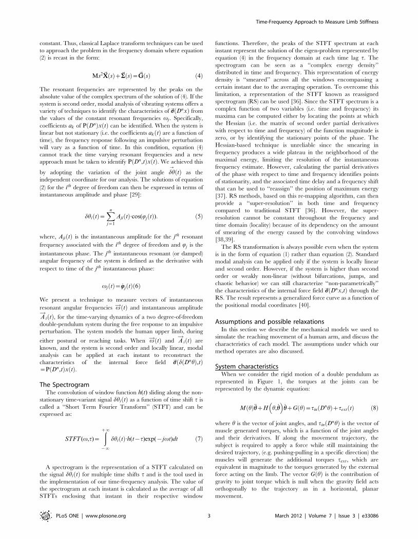
We will now analyze the time-frequency responses of three
viscoelastic mechanical networks with oscillating behaviors. The
schematic of each model is presented in Figure 2 as a single
degree-of freedom (DOF) representation. It is also important to
notice that exact tracking of the arm’s unperturbed trajectory is
not strictly necessary because the parameters are estimated in the
frequency domain.
The system depicted in Figure 2a is commonly known as the
Kelvin-Voigt (KV) model and is widely use to represent the
mechanical behavior of the upper limb. A KV mechanical model
is linear and second order, which allows us to use instantaneous
modal analysis for the identification of system parameters under
several combinations of stiffness and damping time profiles. The
system internal viscoelastic force field f d Dnhð Þ,tð Þ is represented
by the differential equation:
f d D1h� �
,t� �
~{Ch(t):d _hh tð Þ{Kh(t):dh tð Þ ð15Þ
Most identification techniques proposed in the literature assume
the damping Ch and stiffness Kh to be time-invariant. Our work
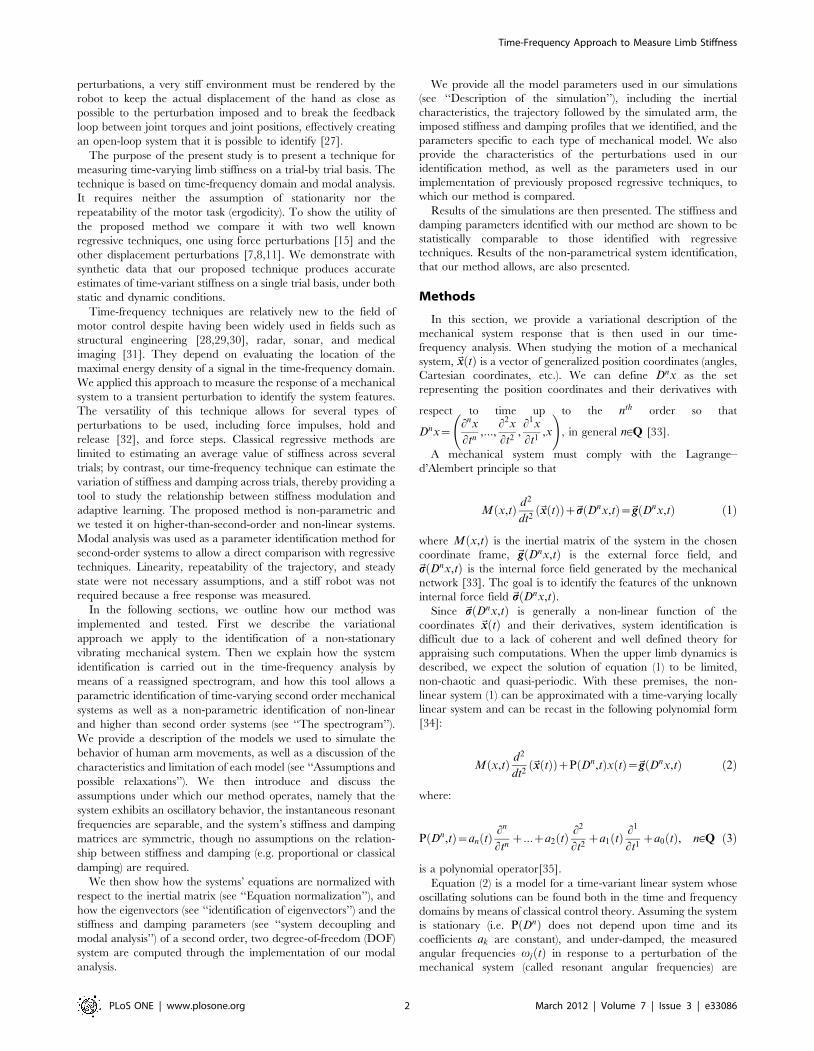
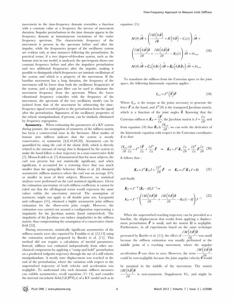
Figure 1. Representation of the double-pendulum model of thearm. The centers of the inertial ellipsoids represented in the figure arelocated at the centers of mass of the body segments. The length of theupper arm is l1 , and the center of mass is at r1 from the shoulder centerof rotation. Hand and forearm are considered as a unit of length l2 withno joint at the wrist. The resulting center of mass for the segment isobtained by the combination of those of the hand and forearm and islocated at r2 from the elbow. The size of each ellipsoid depends onboth mass and inertial tensor of the segment. The dimensions of each
ellipsoid along the major and minor axes (eigenvectors) are computed
as ek~
ffiffiffiffiffiffiffiffiffiffiffiffiffiffiffiffiffiffiffiffiffiffiffiffiffiffi5 tr Ið Þ{2Ik½ �
2m
r, where Ik are the principal moments of inertia of
the tensor I , and m is the mass of the segment. During simulatedmovements, the hand’s center of mass follows the trajectory shown asthe dashed brown line. In the figure the hand center of mass is atposition (0.4,0)m, which is the configuration used for the postural tests.doi:10.1371/journal.pone.0033086.g001
Time-Frequency Approach to Measure Limb Stiffness
PLoS ONE | www.plosone.org 4 March 2012 | Volume 7 | Issue 3 | e33086
relaxes this assumption by considering the coefficients as time-
varying.
Figure 2b represents a linear, time-invariant, third-order system
known as the Poynting-Thomson (PT) model. This mechanical
network is an extension of the KV model commonly used in
muscle models and includes tendon elasticity (Hill-type passive
model). The PT model includes two separate elastic elements. The
element KSh , in series with the muscle fibers, represents the stiffness
of the tendon. The parallel between KPh and CP
h represents the
stiffness and viscosity of the muscle fibers. The internal viscoelatic
field complies with the following differential equation:
f d D3h� �
,t� �
~{KS
h:CP
h
KSh zKP
h
:d _hh tð Þ{ KSh:KP
h
KSh zKP
h
:dh{
CPh
KSh zKP
h
: _ff D3dh,t� � ð16Þ
Figure 2c represents a non-linear system known in the
engineering literature as the Duffing model. It provides an
approximation of a tendon’s slack behavior. Here, the stiffness
depends on position, and is low for small displacements (slacking of
the tendon) and increases abruptly after a fixed threshold. As a first
approximation the stiffness of the model is considered to increase
cubically (hardening system) which is compatible with experimen-
tal evidence found in human triceps surae muscle [42]. In general,
Duffing type models can generate chaotic responses; however, we
will restrict our study to a system with known stable behavior. In
the time domain, Duffing viscoelastic force can be expressed using
the differential equation [43,44]:
f d D1h� �
,t� �
~{Ch:d _hh tð Þ{Kh
:dh tð Þ{Bh: dh tð Þð Þ3 ð17Þ
The generalization to multiple DOFs is easily accomplished, and
results in the parameters KSh ,KP
h ,CPh ,M,Kh,Ch,B which can be
expressed as matrices.
Since modal analysis cannot be used to identify parameters of
PT and Duffing systems, we used the RS technique to identify
non-parametrically the force characteristics of these systems.
Oscillatory behavior. We simulated the mechanics of a
human arm with two coupled degrees of freedom (Figure 2) and
estimated its response to a perturbation using the mechanical
models in equations (15–17). The technique proposed here
requires eliciting an oscillatory response by delivering a
mechanical disturbance to the system. Measurable post-
perturbation oscillations in free space indicate that the arm is an
under-damped mechanical system. Postural measurements and
single joint movement measurements [8,45] also show the
damping to be under-critical. The PT model is physiologically
consistent with muscle-tendon systems and is often used as a linear,
time-invariant approximation. A PT system exhibits one
oscillatory mode, independently of the value of the muscle
damping CPh , if KS
h v8KPh where KS
h is the stiffness of the
tendon and KPh is the stiffness of the muscle fibers. An analytical
proof is presented in Supplement S3. The under-damped PT
model is third-order [46] and has one zero, one real pole, and one
complex pole pair (see Supplement S4). When approximating PT
as a second-order system (i.e. KSh w8KP
h ), oscillating behavior is
still assumed because the complex pole pair must be dominant (if
the real pole were dominant the approximation would be a first-
order system). The approximation to a second-order oscillating
system is accurate when the zero and the single pole have similar
values and their effects cancel out. The double pole dominancy
with respect to both the zero and single pole is supported by
stochastic non-parametric identification [5,47,48]. Given the
ability to approximate the arm as a second-order mechanical
system, the majority of the analysis described here will concentrate
on parameter estimation for KV-type models. We did then
generalize the findings to the more complex PT and Duffing
models.
Separability. We assumed the two instantaneous resonant
frequencies of the system (i.e. the peaks of the spectrogram as a
function of time) to be distinct within the resolution limit of each
transfer function spectrum. The representation of an unperturbed
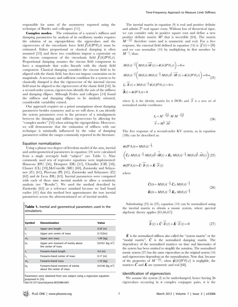
Figure 2. Mechanical models used in the simulations. A) Time-variant second-order viscoelastic linear system (Kelvin-Voigt). B) third-orderviscoelastic linear system (Poynting-Thomson). C) Time-invariant second-order cubic viscoelastic system (Duffing). The schematics highlight thedifferent force fields of the D’Alembert equation (2) when the internal forces generated by the dynamics are negligible. In the figure, each force fieldis dependent to the mechanical elements that generate it.doi:10.1371/journal.pone.0033086.g002
Time-Frequency Approach to Measure Limb Stiffness
PLoS ONE | www.plosone.org 5 March 2012 | Volume 7 | Issue 3 | e33086
movement in the time-frequency domain resembles a function
with a constant value at a frequency the inverse of movement
duration. Impulse perturbations in the time domain appear in the
frequency domain as instantaneous excitations of the entire
frequency spectrum. The characteristic frequency of the
movement is present in the spectrum before and after the
impulse, while the frequencies proper of the oscillatory system
are evident only at time instances following the perturbation. In
practical terms, if a two degree-of-freedom system, such as the
human arm in our model, is analyzed, the spectrogram shows one
constant frequency before and after the impulsive perturbation
and two additional frequencies after the impulse, making it
possible to distinguish which frequencies are intrinsic oscillations of
the system and which is a property of the movement. If the
baseline movement has a long duration, the frequency of the
movement will be lower than both the oscillatory frequencies of
the system, and a high pass filter can be used to eliminate the
movement frequency from the spectrum. When the lower
vibrational frequency coincides with the frequency of the
movement, the spectrum of the two oscillatory modes can be
isolated from that of the movement by subtracting the time-
frequency signal recorded prior to the perturbation from the signal
after the perturbation. Signatures of the oscillatory properties of
the robotic manipulandum, if present, can be similarly eliminated
by frequency segregation.
Symmetry. When estimating the parameters of a KV system
during posture, the assumption of symmetry of the stiffness matrix
has been a controversial issue in the literature. Most studies of
human arm stiffness indicate that the system is mostly
conservative, or symmetric [4,8,10,49,50]. Asymmetry can be
quantified by using the curl of the elastic field, which is directly
related to the amount of energy that is dissipated by the system to
make the hand follow a close trajectory in a non-conservative field
[7]. Mussa-Ivaldi et.al. [7] demonstrated that for most subjects, the
curl was present but not statistically significant, and when
significant, it accounted for a restoring force that was much
smaller than the spring-like behavior. Dolan et al. [6] obtained
asymmetric stiffness matrices where the curl was on average 25%
or smaller in most of their subjects. However, no statistical
analyses were performed on the curl statistical significance. Given
the estimation uncertainty of each stiffness coefficient, it cannot be
ruled out that the off-diagonal terms would represent the same
values within the uncertainty interval. The assumption of
symmetry might not apply to all double joint sets. Lacquaniti
and colleagues [51], obtained a highly asymmetric joint stiffness
estimation for the elbow-wrist joint couple. However, the
estimation was carried out around a configuration representing a
singularity for the Jacobian matrix (hand outstretched). The
singularity of the Jacobian can induce singularities in the stiffness
matrix, thus compromising the assumption of a conservative elastic
field [52].
During movements, statistically significant asymmetries of the
stiffness matrix were also reported by Franklin et al. [12,13] using
the estimation method proposed by Burdet et al. [11]. This
method did not require a calculation of inertial parameters.
Instead, stiffness was estimated independently from other me-
chanical components by applying a ‘‘ramp and hold’’ perturbation
on a predicted endpoint trajectory through the use of a stiff robotic
manipulandum. A steady state displacement was reached at the
end of the perturbation, where the variation with respect to the
unperturbed trajectory of both velocity and acceleration was
negligible. To understand why such dynamic stiffness measures
can exhibit asymmetries, recall equations (11–14), and consider
the internal viscoelastic field f d Dnhð Þ,tð Þ of a KV model such as in
equation (15):
M hð Þ d€hh?
zLH h, _hh� �L _hh
zH h, _hh� �
{Ch tð Þ
0@
1A d _hh
?
z
LM h, _hh� �
€hh
Lhz
LH h, _hh� �
_hh
Lh{Kh tð Þ
0@
1A dh
?~dtext
M hð Þ d€hh?
zCCh h, _hh,t� �
d _hh?
zKKh h, _hh,€hh,t� �
dh?
~dtext
ð18Þ
To transform the stiffness from the Cartesian space to the joint
space, the following kinetostatic equation applies :
~ttext~JT ~hh� �
~FF ð19Þ
Where ~ttext is the torque at the joints necessary to generate the
force ~FF at the hand, and JT hð Þ is the transposed Jacobian matrix,
which is a function of the joint angles ~hh. Knowing that the
Cartesian stiffness is KKX ~L~FFLx
, the Jacobian matrix is J~Lx
Lh, and
from equation (18) that KKh%L~ttext
Lh, we can write the derivative of
the kinetostatic equation with respect to the Cartesian coordinates
~xx so that:
L~ttext
Lh
Lh
Lx~JT L~FF
Lxz
LJT
Lx~FF [ KKh~JT KKx
Lx
Lhz
LJT
Lx~FF
Lx
Lhð20Þ
It follows that :
KKh~JT KKX JzLJT
Lh~FF [ KKh~JT KKX JzV ð21Þ
and finally
KKX ~J{T KKh{V� �
J{1[
KX ~J{TLM h, _hh
� �€hh
Lhz
LH h, _hh� �
_hh
Lh{Kh tð Þ{V
0@
1AJ{1
ð22Þ
When the unperturbed reaching trajectory can be provided as a
baseline, the displacement that results from applying a displace-
ment perturbation ~FF is small, and the matrix V is negligible.
Furthermore, in all experiments based on the same technique
presented by Burdet et al. [11], the effect ofLM h, _hh� �
€hh
Lhwas small
because the stiffness estimation was usually performed at the
middle point of a reaching movement, where the angular
acceleration €hh was close to zero. However, the termLH h, _hh� �
_hh
Lhcould be non-negligible because the joint angular velocity _hh would
be maximal in the middle of the movement. The matrix
LH h, _hh� �
_hh
Lhis non-symmetric (Supplement S1), and might be
Time-Frequency Approach to Measure Limb Stiffness
PLoS ONE | www.plosone.org 6 March 2012 | Volume 7 | Issue 3 | e33086
responsible for some of the asymmetry reported using the
technique of Burdet and colleagues [11].
Complex modes. The estimation of a system’s stiffness and
damping parameters by analysis of its oscillatory modes requires
the solution of an eigenproblem: the eigenvalues and the
eigenvectors of the viscoelastic force field ~ff d Dnhð Þ,tð Þ must be
estimated. Either proportional or classical damping is often
assumed [53] and these two conditions impose a constraint on
the viscous component of the viscoelastic field ~ff d Dnhð Þ,tð Þ.Proportional damping assumes the viscous field component to
have a magnitude that scales linearly with the elastic field
component. Classical damping considers the viscous field to be
aligned with the elastic field, but does not impose constraints on its
magnitude. A necessary and sufficient condition for a system to be
classically damped is that the eigenvector of the internal viscous
field must be aligned to the eigenvectors of the elastic field [54]. In
a second-order system, eigenvectors identify the axis of the stiffness
and damping ellipses. Although Frolov and collegues [14] found
the stiffness and damping ellipses to be similarly oriented,
considerable variability existed.
Our approach requires no a priori assumptions about damping
parameters besides symmetry and as we will show, it can identify
the system parameters even in the presence of a misalignment
between the damping and stiffness eigenvectors by allowing for
‘‘complex modes’’ [55] when solving the eigenproblem. Moreover,
we will demonstrate that the estimation of stiffness with our
technique is minimally influenced by the value of damping
parameters within the ranges commonly reported in the literature.
Equation normalizationUsing a planar two degree-of-freedom model of the arm, inertial
and anthropometrical parameters in equation (10) were calculated
from a single averagely built ‘‘subject’’ (see Table 1). Nine
commonly used sets of regressive equations were implemented:
Hanavan (HV) [56], Dempster (DE) [57], Chandler (CH) [58],
Clauser (CL) [59],McConville (MC) [60], Zatsiorsky and Seluya-
nov (Z1) [61], Piovesan (PI) [41], Zatsiorsky and Seluyanov (Z2)
[62] and de Leva (DL) [63]. Inertial parameters were computed
with each of these nine inertial models to allow a sensitivity
analysis (see ‘‘Results’’). We used the method described by
Zatsiorsky [62] as a reference standard because we had found
earlier [41] that this method best approximates the true inertial
parameters across the aforementioned set of inertial models.
The inertial matrix in equation (9) is real and positive definite
and admits 2n real square roots. Without loss of theoretical rigor,
we can consider only its positive square root and define a new
positive definite matrix M12 that is invertible [64]. The matrix
M{ 12ð Þ therefore exists and is symmetric and real. For a free
response, the external field defined in equation (14) is g! tð Þ~ 0f gand we can normalize (14) by multiplying its first member by
M{12, thus:
M(h,t){1
2 M(h,t) d€hh�!
tð Þz~ss d Dnhð Þ,tð Þ�
~0[
M(h,t){1
2 M(h,t):M(h,t){1
2:M(h,t)12: d€hh�!
tð Þz~ss d Dnhð Þ,tð Þ�
~0[
In: €qq!
tð ÞzM(h,t){1
2:~ss d Dnhð Þ,tð Þ~0[
~€qq€qq tð Þz~ss(Dnq,t)~0
ð23Þ
where In is the identity matrix for n DOFs and q!
is a new set of
normalized modal coordinates
In~M{ 1
2
� �:M:M{ 1
2
� �q!
~M12: dh�! ð24Þ
The free response of a second-order KV system, as in equation
(18b) can be described as:
~ss(Dnq,t)~M(h,t){1
2:
CCh:M(h,t)
{12:M(h,t)
12: d _hh
?
tð ÞzKKh:M(h,t)
{12:M(h,t)
12: dh
?tð Þ
�
~ss(Dnq,t)~~CC: _qq!
tð Þz ~KK : q!
tð Þ
ð25Þ
where
~CC(t)~M(h,t){1
2:CCh:M(h,t)
{12
~KK(t)~M(h,t){1
2:KKh:M(h,t){
12
ð26Þ
Substituting (25) in (23), equation (14) can be normalized using
the inertial matrix to obtain a monic system, where spectral
algebraic theory applies [65,66,67]:
€qq!
tð Þz~CC: _qq!
tð Þz ~KK : q!
tð Þ~0 ð27Þ
~KK is the normalized stiffness also called the ‘‘system matrix’’ or the
‘‘modal matrix’’, ~CC is the normalized damping matrix. The
dependency of the normalized matrices on time and kinematics of
the system has been omitted to simplify the notation. The normalized
monic system (27) has the same eigenvalues as the original system (14)
and eigenvectors dependent on the normalization. Note that, because
of the properties of M{ 12ð Þ, when ~yy d D1h
� �,t
� �is negligible, the
matrices ~CC and ~KK are symmetric and real [68].
Identification of eigenvectorsWe assume the system (2) to be underdamped, hence having 2n
eigenvalues occurring in n complex conjugate pairs, n is the
Table 1. Inertial and geometrical parameters used in thesimulations.
Symbol Denomination Value
l1 Upper arm length 0.29 [m]
r1 Upper arm center of mass 0.132[m]
m1 Upper arm mass 1.99 [kg]
Iz1 Upper arm moment of inertia aboutthe center of mass
0.0161 [kg m2]
l2 Forearm+hand length 0.4 [m]
r2 Forearm+hand center of mass 0.17 [m]
m2 Forearm+hand mass 1.10 [kg]
Iz2 Forearm+hand moment of inertiaabout the center of mass
0.0146 [kg m2]
Parameters were obtained from one subject using a regression equationproposed in [55].doi:10.1371/journal.pone.0033086.t001
Time-Frequency Approach to Measure Limb Stiffness
PLoS ONE | www.plosone.org 7 March 2012 | Volume 7 | Issue 3 | e33086
number of DOFs:
lj~ajzivj
�llj~aj{ivj
ð28Þ
where j = [1,2] for a two DOF system. In the general case of non-
classically damped system, if ~vvj is the eigenvector associated with
lj , the corresponding eigenvector of �llj will simply be the complex
conjugate �~vv~vvj [55]. A linear combination of the eigen-solutions
represents a general solution to (2):
~ssj~aj~vvjelj t
zbj�~vv~vvje
�llj t ð29Þ
If the system is classically damped, all the eigenvectors of the
system will be real [55,69], so that:
~ppj~~vvj~�~vv~vvj ð30Þ
and the matrix of the system eigenvectors can be written as:
P~
p11� � � pj1
� � � pn1
p12
..
.
� � �
P
pj2
..
.
� � �
P
pn2
..
.
p1n � � � pjn � � � pnn
2666664
3777775!
P1~
1
p12
.p11
� � �
� � �
1
pj2
.pj1
� � �
� � �
1
pn2
.pn1
..
.P
..
.P
..
.
p1n
.p11
� � � pjn
.pj1
� � � pnn
.pn1
266666664
377777775
ð31Þ
In P the magnitude of each vector is normalized to 1, and in P1
the first component of the vector is normalized to 1.
To be a physically possible solution, each sj in equation (29)
must be real, hence bj~�aaj [55], therefore:
~ssj~Re 2aj pI
jelj t
� �~2 Re aj p
Ije
ajzivj
� �t
� ~
2 Re ajeajzivj
� �t
� pI
j
ð32Þ
In general aj is a complex number and it can be written in the
exponential form 2aj~Cje{iwj , with Cj and wj real [55].
After substitution, (32) can be written as:
~ssj~Cjeaj tRe ei vj t{wj
� �� pI
j~
~Cjeaj t Re cos vj t{wj
� �zi sin vj t{wj
� �� �~Cje
aj t cos vj t{wj
� �pI
j
ð33Þ
The general solution of (2), or the linear combination of all the
solutions of the eigenproblem, can be interpreted as the super-
position of each damped mode of vibration [55], and in general
can be written in the form:
dh�!
~Xn
j~1
aj~vvjelj t
zbj�~vv~vvje
�llj t� �
~Xn
j~1
~ssj ð34Þ
Since (2) is not decoupled, the free time response of each degree
of freedom will be of the form (34). If the instantaneous reassigned
frequencies are sufficiently far apart from each other (separable in
the frequency domain), then each independent damped mode can
be isolated at each instant using a filtering process. Each dhi is
high-pass and low-pass filtered within a sliding window h(t{t), at
a cutoff frequency located at the average between adjacent
instantaneous frequencies derived from the RS within the same
window. In our case (a two DOF system), using (33) and (34) we
obtain: vc(t{t)~v1zv2
2. For convenience the window and the
hop size are the same as those used for computing the
spectrogram.
dh1
dh2
( )~~ss1z~ss2~
s11
s12
( )z
s21
s22
( )~
C1ea1t cos v1t{w1ð Þp11
p12
( )zC2ea2t cos v2t{w2ð Þ
p21
p22
( ) ð35Þ
Recalling (5) we can see that
dh1
dh2
�~
A11 tð Þ:cos(Q1 tð Þ)zA21 tð Þ: cos (Q2 tð Þ)A21 tð Þ: cos (Q1 tð Þ)zA22 tð Þ: cos (Q2 tð Þ)
�ð36Þ
and from (35) and (36) that
p11
p12
~A11
A12and
p21
p22
~A21
A22ð37Þ
Each time-varying eigenvector in P1 can be calculated as the
ratio between the instantaneous amplitude of each modal
coordinate’s mode.
If the system has complex modes, the eigenvectors of the system
will be complex and can be represented in the form:
~vvj~ pj1e{icj1 pj2
e{icj2 . . . pjn e{icjn
h iT
ð38Þ
Substituting (38) in (33), each mode can assume the following
general form:
~ssj~Cjeaj t cos vj t{wj
� �pj1
e{icj1 pj2
e{icj2 . . . pjn e{icjn
h iT
ð39Þ
A physical interpretation of this formulation is that the jth mode
oscillates with frequency vj and decays with a damping ratio aj ,
and each of its kth components presents a phase shift of cjk.
In the case of a two DOF system, equation (39) can be written
as:
Time-Frequency Approach to Measure Limb Stiffness
PLoS ONE | www.plosone.org 8 March 2012 | Volume 7 | Issue 3 | e33086
dh1
dh2
( )~
s11
s12
( )z
s21
s22
( )~C1ea1t cos v1t{w1ð Þ
p11e{ic11
p12e{ic12
8<:
9=;zC2ea2t cos v2t{w2ð Þ
p21e{ic21
p22e{ic22
8<:
9=;
ð40Þ
It follows from (40) that:
v11
v12
~p11
e{ic11
p12e{ic12
~A11
A12cos(c12
{c11)
andv21
v22
~p21
e{ic21
p22e{ic22
~A21
A22cos(c22
{c21)
ð41Þ
The difference in phase between sj1 and sj2 is then rj~cj2{cj1
[40]. Because sj1 and sj2 are time signals with the same frequency,
the time lag between the two is equal to:
Dj~rj
vj
ð42Þ
Dj can be found using a cross-correlation function between the
components of each mode characterized by the same frequency.
For a 2 DOF system, when ~KK and ~CC are symmetric, r1~{r2,
we will show that rj is equal to half the rotation of the damping
matrix eigenvectors with respect to the stiffness matrix eigenvec-
tors. If the system is assumed to be non-symmetric, each ri should
be identified independently.
System Decoupling and Modal AnalysisThe signals ~vv tð Þ and ~AAj tð Þ are related to the coefficients that
decouple equation (2). Assuming the system linear and second
order, the values of the matrices Kh and Ch, representing stiffness
and damping respectively, can be estimated from the decoupled
system (eigenproblem solution) under the hypothesis of an under-
damped mechanism with known inertial parameters (‘‘inverse
problem’’). The solution of the inverse problem requires that the
eigenvectors and eigenvalues of the system be known. While the
eigenvalues can easily be obtained from a spectrogram since they
uniquely represent the resonant frequencies of the system, the
eigenvector (i.e. the modes of vibration) must be reconstructed
from the measured data in a convenient modal reference frame. In
a symmetric classically damped system, the eigenvectors for both
the normalized stiffness and normalized damping in (27) are the
same, and can be reconstructed from the instantaneous amplitude
of the spectrogram. In a non-classically damped system, a further
step is necessary to estimate the phase difference r between the
modes. Once the matrix of eigenvectors P is estimated we can use
its properties to decouple the normalized system (27) so that:
PT :P~In
PT :~KK :P~LK~diag½g2j �
PT :~CC:P~LC~diag½2Cj �
ð43Þ
where g2j tð Þ is the eigenvalue of ~KK which corresponds to the jth
squared ‘‘natural’’ or ‘‘undamped’’ angular frequency, and Cj(t) is
the eigenvalue of ~CC corresponding to the jth universal damping
ratio. Therefore, equation (27) can be rewritten as follows:
€qq!
tð ÞzLC: _qq!
tð ÞzLK: q!
tð Þ~0 ð44Þ
If the instantaneous ‘‘resonant’’ angular frequencies vj tð Þ are
not constant, then the normalized squared ‘‘natural’’ angular
frequency g2j tð Þ and the universal damping ratio Cj(t) associated to
each of the jth vibrational modes are time-varying and can be
estimated as follows [40,70]:
Cj(t)~{aj{_vvj
2vj
ð45Þ
g2j tð Þ~v2
j za2j z
aj _vvj
vj
{ _aaj ð46Þ
where
aj tð Þ~ d
dtln Aj(t)� �
~_AAj(t)
Aj(t): ð47Þ
If the system is second-order, by knowing the matrix P we can
reconstruct (27) from (44), and by having defined M{ 1
2
� �we can
compute (2) from (27), obtaining an estimation of the stiffness KK
and damping CC in the time domain, namely:
KK~M12:P:diag½g2
j �:PT :M12
CC~M12:P:diag½2C j �:PT :M
12
ð48Þ
Furthermore, by knowing ~yy(D1dh,t), Kh and Ch can be readily
estimated from (18).
The parametric modal analysis here described cannot be
applied to Duffing or PT models. However, spectral decomposi-
tion is still possible given the oscillatory behavior of the system.
Hence it is still possible to identify the instantaneous resonant
frequency vj tð Þ and amplitude ~AAj tð Þ for each degree of freedom.
Equations (45–47) still apply, therefore we can estimate the
features of the internal force [71].
~ss1(Dnq,t)~g1:A1z2C1
: _AA1 ~ss2(Dnq,t)~g2:A2z2C2
: _AA2 qw0
~ss1(Dnq,t)~{g1:A1{2C1
: _AA1 ~ss2(Dnq,t)~{g2:A2{2C2
: _AA2 qv0ð49Þ
Description of the SimulationA planar two degree-of-freedom model of the arm was used to
analyze both static postural and reaching movement conditions
(Figure 1). The model was implemented using SimulinkH (The
MathworksH, Natick, MA). During simulations of arm movement,
the center of mass of the hand followed an imposed straight
trajectory on the horizontal plane, parallel to the sagittal plane.
The origin of the reference system was placed at the center of
rotation of the shoulder with x axis parallel to the direction of
movement and positive distally and the y axis positive medially.
The starting position at t = 0 was at a point (0.25,0)m in front of
Time-Frequency Approach to Measure Limb Stiffness
PLoS ONE | www.plosone.org 9 March 2012 | Volume 7 | Issue 3 | e33086
the shoulder, and the target was located at point (0.55,0)m
(Figure 1).
The hand trajectory varied sigmoidally in time described by the
equation:
x tð Þ~ G
(1zQ:e{B:(t{E))zD
y(t)~0
ð50Þ
where
G~x(T){x(0); B~4; Q~1; D~x(0); E~T=2 ð51Þ
We used T~5s of simulated time, with sampling at 4 kHz, to
allow the sigmoid to start with zero curvature. Effective movement
duration was Teff ~1s, defined as the time between 10 and 90% of
the total amplitude G (Figure 3a). Dynamic stiffness was tested
between (0.4,0)m and (0.55,0)m in the second half of the
trajectory, between time T = 2.5 s and T = 5 s during the
movement. Postural time-varying stiffness was tested in the same
time interval with the hand at point (0.4,0)m which corresponded
to the center of the simulated reach.
Time-variant Kelvin-Voigt System. For both the postural
and the movement simulated paradigms, the reference joint
stiffness and damping were set at
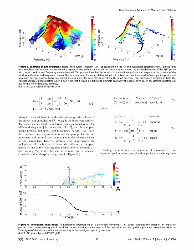
Figure 3. Representation of the imposed reaching trajectoryand the multipliers for the stiffness time profiles. In the leftpanel, the reaching profile for the x (solid) and y (dashed dotted)components of movement are represented using the convention ofFigure 1. The co-ordinates shown in light blue refer to the position ofthe hand’s center of mass used in the static (postural) condition. For thefirst part of the trajectory, a constant stiffness and damping areimposed at the beginning of the movement (right panel). Subsequent-ly, after the application of a force impulse perturbation, the jointstiffness is modulated by means of the gain profiles depicted on theright panel. We imposed a constant (green), slow sigmoidal (red), acombination of linear and sinusoidal (blue), and sharp sigmoidal gain(black), respectively. The same time-varying profiles are also imposed tostiffness and damping during the simulated static condition.doi:10.1371/journal.pone.0033086.g003
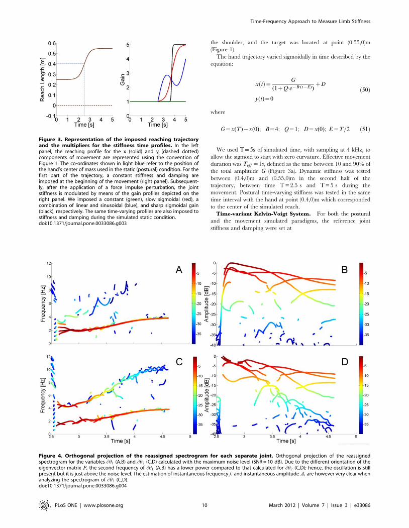
Figure 4. Orthogonal projection of the reassigned spectrogram for each separate joint. Orthogonal projection of the reassignedspectrogram for the variables Lh1 (A,B) and Lh2 (C,D) calculated with the maximum noise level (SNR = 10 dB). Due to the different orientation of theeigenvector matrix P, the second frequency of Lh1 (A,B) has a lower power compared to that calculated for Lh2 (C,D); hence, the oscillation is stillpresent but it is just above the noise level. The estimation of instantaneous frequency fi and instantaneous amplitude Ai are however very clear whenanalyzing the spectrogram of Lh2 (C,D).doi:10.1371/journal.pone.0033086.g004
Time-Frequency Approach to Measure Limb Stiffness
PLoS ONE | www.plosone.org 10 March 2012 | Volume 7 | Issue 3 | e33086
K0~k11 k12
k21 k22
" #~
35 5
5 20
" #Nm=rad
C0~0:01:K0 Nms=rad
ð52Þ
where k11 is the stiffness of the shoulder joint, k22 is the stiffness of
the elbow joint variables, and k12~k21 is the intra-joint stiffness.
The values chosen for the simulation match published values for
stiffness during multijoint movements [11,15], and for damping
during postural and single joint movements [6,8,45]. We tested
three separate time-varying stiffness and damping profiles for the
movement and postural cases by modulating the reference values
of the parameters. Different profiles were implemented by
multiplying all coefficients of either the stiffness or damping
matrix by one of the following time-profiles u(t): a ‘‘constant’’, a
slow varying ‘‘sigmoid’’, the sum of a ramp and a sinusoid
(‘‘sinlin’’), and a ‘‘sharp’’ varying sigmoid (Figure 3b):
Kh(t)~K0:ur(t) ½Nm=rad� 2:5ƒtƒT
Ch(t)~C0:us(t) ½Nms=rad� r,s~1,::,4
ð53Þ
where
u1 tð Þ~1 constant
u2 tð Þ~ 4
(1ze{4:(t{3T
4))z1 sigmoid
u3 tð Þ~sin(4
5pt)z
8
5t{4 sinlin
u4 tð Þ~ 4
(1ze{30:(t{3T
4))z1 sharp
ð54Þ
Finding the stiffness at the beginning of a movement is an
important goal in motor-control and might help in shedding some
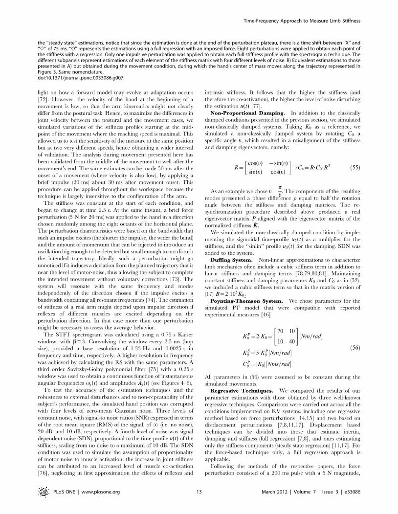
Figure 5. Example of Spectrograms. Short Time Fourier Transform (STFT) Spectrogram on the left and Reassigned Spectrogram (RS) on the rightfor a simulated arm reaching movement with sigmoidal joint stiffness. Based on the classical spectrogram, the partial derivatives of the STFT phasewith respect to time and frequency were calculated. This process identifies the location of the stationary phase with respect to the location of thewindow in the time and frequency domain. The time delay and frequency shift obtained with this process are then used to ‘‘reassign’ the position ofmaximum energy. Savitzky-Golay polynomial filtering allows for easy calculation of the RS peaks envelope. The envelope is depicted in both theclassical and reassigned spectrogram in black. Note that it would be difficult to estimate accurately the peaks’ envelope in the classical spectrogramdue to the lower frequency accuracy.doi:10.1371/journal.pone.0033086.g005
Figure 6. Frequency separation. A) Reassigned spectrogram of a perturbed movement. This panel illustrates the effect of an impulsiveperturbation on the spectrogram of the elbow angular rotation, the frequency of the oscillations excited by the impulse are clearly identifiable. B)Time signal of the elbow rotation corresponding to the reassigned spectrogram in A).doi:10.1371/journal.pone.0033086.g006
Time-Frequency Approach to Measure Limb Stiffness
PLoS ONE | www.plosone.org 11 March 2012 | Volume 7 | Issue 3 | e33086
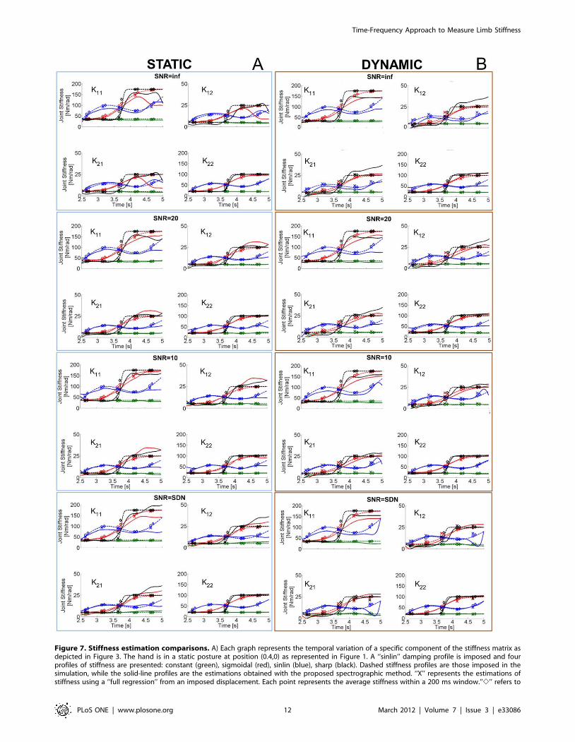
Figure 7. Stiffness estimation comparisons. A) Each graph represents the temporal variation of a specific component of the stiffness matrix asdepicted in Figure 3. The hand is in a static posture at position (0.4,0) as represented in Figure 1. A ‘‘sinlin’’ damping profile is imposed and fourprofiles of stiffness are presented: constant (green), sigmoidal (red), sinlin (blue), sharp (black). Dashed stiffness profiles are those imposed in thesimulation, while the solid-line profiles are the estimations obtained with the proposed spectrographic method. ‘‘X’’ represents the estimations ofstiffness using a ‘‘full regression’’ from an imposed displacement. Each point represents the average stiffness within a 200 ms window.’’e’’ refers to
Time-Frequency Approach to Measure Limb Stiffness
PLoS ONE | www.plosone.org 12 March 2012 | Volume 7 | Issue 3 | e33086
light on how a forward model may evolve as adaptation occurs
[72]. However, the velocity of the hand at the beginning of a
movement is low, so that the arm kinematics might not clearly
differ from the postural task. Hence, to maximize the differences in
joint velocity between the postural and the movement cases, we
simulated variations of the stiffness profiles starting at the mid-
point of the movement where the reaching speed is maximal. This
allowed us to test the sensitivity of the measure at the same position
but at two very different speeds, hence obtaining a wider interval
of validation. The analysis during movement presented here has
been validated from the middle of the movement to well after the
movement’s end. The same estimates can be made 50 ms after the
onset of a movement (where velocity is also low), by applying a
brief impulse (20 ms) about 30 ms after movement onset. This
procedure can be applied throughout the workspace because the
technique is largely insensitive to the configuration of the arm.
The stiffness was constant at the start of each condition, and
began to change at time 2.5 s. At the same instant, a brief force
perturbation (5 N for 20 ms) was applied to the hand in a direction
chosen randomly among the eight octants of the horizontal plane.
The perturbation characteristics were based on the bandwidth that
such an impulse excites (the shorter the impulse, the wider the band)
and the amount of momentum that can be injected to introduce an
oscillation big enough to be detected but small enough to not disturb
the intended trajectory. Ideally, such a perturbation might go
unnoticed if it induces a deviation from the planned trajectory that is
near the level of motor-noise, thus allowing the subject to complete
the intended movement without voluntary corrections [73]. The
system will resonate with the same frequency and modes
independently of the direction chosen if the impulse excites a
bandwidth containing all resonant frequencies [74]. The estimation
of stiffness of a real arm might depend upon impulse direction if
reflexes of different muscles are excited depending on the
perturbation direction. In that case more than one perturbation
might be necessary to assess the average behavior.
The STFT spectrogram was calculated using a 0.75 s Kaiser
window, with b= 3. Convolving the window every 2.5 ms (hop
size), provided a base resolution of 1.33 Hz and 0.0025 s in
frequency and time, respectively. A higher resolution in frequency
was achieved by calculating the RS with the same parameters. A
third order Savitzky-Golay polynomial filter [75] with a 0.25 s
window was used to obtain a continuous function of instantaneous
angular frequencies vj(t) and amplitudes ~AAj(t) (see Figures 4–6),
To test the accuracy of the estimation techniques and the
robustness to external disturbances and to non-repeatability of the
subject’s performance, the simulated hand position was corrupted
with four levels of zero-mean Gaussian noise. Three levels of
constant noise, with signal-to noise ratios (SNR) expressed in terms
of the root mean square (RMS) of the signal, of ? (i.e. no noise),
20 dB, and 10 dB, respectively. A fourth level of noise was signal
dependent noise (SDN), proportional to the time-profile u(t) of the
stiffness, scaling from no noise to a maximum of 10 dB. The SDN
condition was used to simulate the assumption of proportionality
of motor noise to muscle activation: the increase in joint stiffness
can be attributed to an increased level of muscle co-activation
[76], neglecting in first approximation the effects of reflexes and
intrinsic stiffness. It follows that the higher the stiffness (and
therefore the co-activation), the higher the level of noise disturbing
the estimation u(t) [77].
Non-Proportional Damping. In addition to the classically
damped conditions presented in the previous section, we simulated
non-classically damped systems. Taking K0 as a reference, we
simulated a non-classically damped system by rotating C0 a
specific angle u, which resulted in a misalignment of the stiffness
and damping eigenvectors, namely:
R~cos(u) {sin(u)
sin(u) cos(u)
� ?Cu~R:C0
:RT ð55Þ
As an example we chose u~p
6. The components of the resulting
modes presented a phase difference r equal to half the rotation
angle between the stiffness and damping matrices. The re-
synchronization procedure described above produced a real
eigenvector matrix P aligned with the eigenvector matrix of the
normalized stiffness ~KK .
We simulated the non-classically damped condition by imple-
menting the sigmoidal time-profile u2 tð Þ as a multiplier for the
stiffness, and the ‘‘sinlin’’ profile u3 tð Þ for the damping. SDN was
added to the system.
Duffing System. Non-linear approximations to characterize
limb mechanics often include a cubic stiffness term in addition to
linear stiffness and damping terms [78,79,80,81]. Maintaining
constant stiffness and damping parameters K0 and C0 as in (52),
we included a cubic stiffness term so that in the matrix version of
(17) B~2:105K0.
Poynting-Thomson System. We chose parameters for the
simulated PT model that were compatible with reported
experimental measures [46]
KPh ~2:K0~
70 10
10 40
" #Nm=rad½ �
KSh ~5:KP
h Nm=rad½ �
CPh ~ K0j j Nms=rad½ �
ð56Þ
All parameters in (56) were assumed to be constant during the
simulated movements.
Regressive Techniques. We compared the results of our
parameter estimations with those obtained by three well-known
regressive techniques. Comparisons were carried out across all the
conditions implemented on KV systems, including one regressive
method based on force perturbations [14,15] and two based on
displacement perturbations [7,8,11,17]. Displacement based
techniques can be divided into those that estimate inertia,
damping and stiffness (full regression) [7,8], and ones estimating
only the stiffness components (steady state regression) [11,17]. For
the force-based technique only, a full regression approach is
applicable.
Following the methods of the respective papers, the force
perturbation consisted of a 200 ms pulse with a 5 N magnitude,
the ‘‘steady state’’ estimations, notice that since the estimation is done at the end of the perturbation plateau, there is a time shift between ‘‘X’’ and‘‘e’’ of 75 ms. ‘‘O’’ represents the estimations using a full regression with an imposed force. Eight perturbations were applied to obtain each point ofthe stiffness with a regression. Only one impulsive perturbation was applied to obtain each full stiffness profile with the spectrogram technique. Thedifferent subpanels represent estimations of each element of the stiffness matrix with four different levels of noise. B) Equivalent estimations to thosepresented in A) but obtained during the movement condition, during which the hand’s center of mass moves along the trajectory represented inFigure 3. Same nomenclature.doi:10.1371/journal.pone.0033086.g007
Time-Frequency Approach to Measure Limb Stiffness
PLoS ONE | www.plosone.org 13 March 2012 | Volume 7 | Issue 3 | e33086
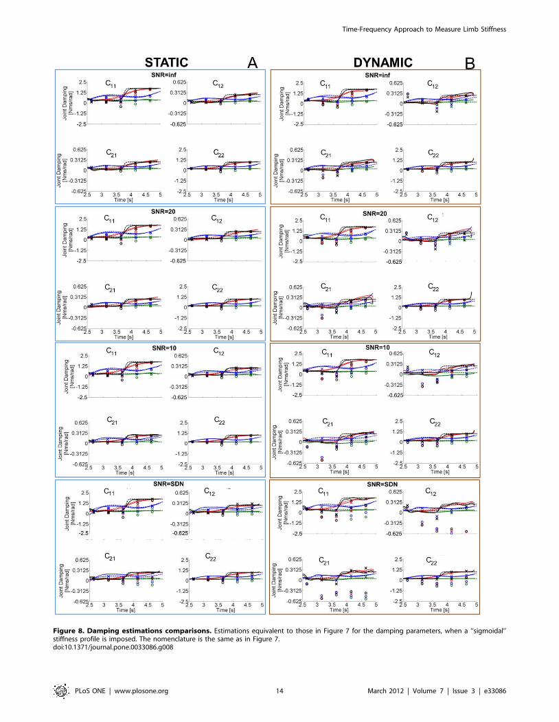
Figure 8. Damping estimations comparisons. Estimations equivalent to those in Figure 7 for the damping parameters, when a ‘‘sigmoidal’’stiffness profile is imposed. The nomenclature is the same as in Figure 7.doi:10.1371/journal.pone.0033086.g008
Time-Frequency Approach to Measure Limb Stiffness
PLoS ONE | www.plosone.org 14 March 2012 | Volume 7 | Issue 3 | e33086
while the displacement perturbations were a deviation from the
unperturbed trajectory with a maximum amplitude of 8 mm,
lasting 300 ms (100 ms ramp-up, 100 ms plateau, 100 ms ramp-
down about the unperturbed trajectory). To have the same
number of points per estimate for both the force-based and
displacement–based full regressions, only the first 200 ms of the
displacement perturbations was used to compute the regression
with the reaction force.
When full regression methods are used to estimate stiffness and
damping during movements, even though inertial properties can be
directly measured, they are usually evaluated in a separate static
session to reduce the number of parameters to estimate at once
[6,15]. This approach is possible because inertial parameters are
invariant with respect to the segments’ centers of mass as seen in (10).
Methods that consider regressions at steady state [11] provide
estimates of stiffness that are independent of the inertial
parameters once particular conditions are met. As previously
mentioned, estimating stiffness independently from the other
mechanical components is possible toward the end of the
perturbation plateau. In such a condition, if the robot is quite
stiff, the variation with respect to the unperturbed trajectory of
both velocity and acceleration is negligible, and the displacement
reaches steady state. However, as seen in equation (18), this
approximation might not be applicable at each point of the
trajectory, especially if the stiffness is measured in positions with
maximal acceleration. When we implemented this procedure in
our simulations the last 50 ms of the plateau region was
considered.
We estimated stiffness and damping at five different instants
along the trajectory, starting at 2.5 s and then every 0.5 s. The
actual location of each point of stiffness estimation depended on
the methods specific to each technique. For each time-point
estimation, one perturbation in eight different directions was used,
resulting in a total of forty trials per method, for each of the four
noise levels. We assumed the unperturbed trajectory to be known
exactly. To compare directly the time discrete stiffness and
damping profiles provided by each regressive method with the
continuous estimation of the spectrogram method, we interpolated
the punctual stiffness using a cubic Hermite spline. This method
guaranteed a unique representation of each time-profile.
Results
The parameter estimation of multiple stiffness and damping
profiles carried out with our time-frequency technique described in
the ‘‘Methods’’ section is compared to the identification of the
same parameters with previously proposed regressive techniques.
A non-parametric identification of higher than second order and
non-linear systems is also provided.
Identification of instantaneous frequencies andamplitudes
As implicit in equations (35) and (40), the time-frequency
representation of the elicited vibrations Lh1 at the shoulder, and
dh2 at the elbow, exhibit the same instantaneous frequencies
fj(t)~2pvj(t), and amplitude decay Aj(t) depending on the
orientation of eigenvector matrix P, since the general free response
to a perturbation is a superimposition of the two modes. This is
evident in Figure 4 where the spectrograms of dh1 and dh2 are
depicted. The higher vibrational frequency is better defined in the
spectrogram of dh2. Since in the proposed simulated paradigm,
the eigenvector component p21is small, so too is the energy
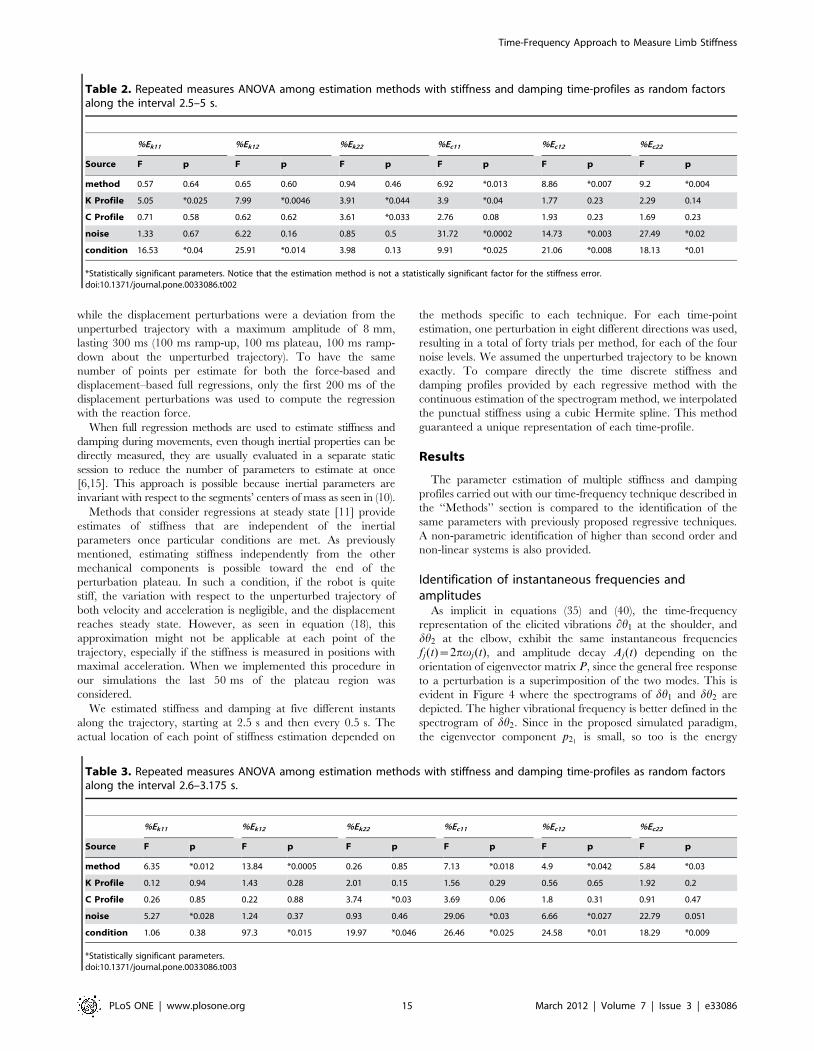
Table 2. Repeated measures ANOVA among estimation methods with stiffness and damping time-profiles as random factorsalong the interval 2.5–5 s.
%Ek11 %Ek12 %Ek22 %Ec11 %Ec12 %Ec22
Source F p F p F p F p F p F p
method 0.57 0.64 0.65 0.60 0.94 0.46 6.92 *0.013 8.86 *0.007 9.2 *0.004
K Profile 5.05 *0.025 7.99 *0.0046 3.91 *0.044 3.9 *0.04 1.77 0.23 2.29 0.14
C Profile 0.71 0.58 0.62 0.62 3.61 *0.033 2.76 0.08 1.93 0.23 1.69 0.23
noise 1.33 0.67 6.22 0.16 0.85 0.5 31.72 *0.0002 14.73 *0.003 27.49 *0.02
condition 16.53 *0.04 25.91 *0.014 3.98 0.13 9.91 *0.025 21.06 *0.008 18.13 *0.01
*Statistically significant parameters. Notice that the estimation method is not a statistically significant factor for the stiffness error.doi:10.1371/journal.pone.0033086.t002
Table 3. Repeated measures ANOVA among estimation methods with stiffness and damping time-profiles as random factorsalong the interval 2.6–3.175 s.
%Ek11 %Ek12 %Ek22 %Ec11 %Ec12 %Ec22
Source F p F p F p F p F p F p
method 6.35 *0.012 13.84 *0.0005 0.26 0.85 7.13 *0.018 4.9 *0.042 5.84 *0.03
K Profile 0.12 0.94 1.43 0.28 2.01 0.15 1.56 0.29 0.56 0.65 1.92 0.2
C Profile 0.26 0.85 0.22 0.88 3.74 *0.03 3.69 0.06 1.8 0.31 0.91 0.47
noise 5.27 *0.028 1.24 0.37 0.93 0.46 29.06 *0.03 6.66 *0.027 22.79 0.051
condition 1.06 0.38 97.3 *0.015 19.97 *0.046 26.46 *0.025 24.58 *0.01 18.29 *0.009
*Statistically significant parameters.doi:10.1371/journal.pone.0033086.t003
Time-Frequency Approach to Measure Limb Stiffness
PLoS ONE | www.plosone.org 15 March 2012 | Volume 7 | Issue 3 | e33086
content transferred from the perturbation to s21(the component of
the 2nd mode along the 1st DOF).
Figure 5a, represents an example of a three dimensional view of
the union between the spectrograms of dh1 and dh2. The regular
STFT spectrogram representation and its reassignment can be
compared. The RS enhances the resolution of the spectrogram
and allows for a better identification of the instantaneous
frequencies fj(t), and amplitude decay Aj(t), despite the presence
of some easily identifiable computational artifacts. The figure also
shows fj(t) and Aj(t) as functions of time, obtained with the
polynomial filtering of the RS.
An example of an unfiltered reassigned spectrogram (RS) of a
movement perturbed by an impulsive force is presented in
Figure 6. In the time-frequency domain, an impulsive perturbation
appears as a constant in the frequency domain (Figure 6a). This
means that when an impulse is applied to a mechanical system, all
the frequencies will be excited with approximately the same
power. The instantaneous frequencies of the vibrational modes
arise immediately after the impulse response. Figure 6b presents
the time profile of elbow rotation h2 with the impulsive
perturbation occurring at the movement middle point.
Estimation of the Stiffness and Damping MatricesTo quantify the sensitivity of our method with respect to
parameters of the mechanical model and to compare our results
with those of published regressive techniques, we analyzed the
performance of each method across a range of different parameter
configurations. Stiffness and damping profiles were estimated in
both static (postural) and dynamic conditions. As an example of the
estimation, Figure 7 depicts the estimated stiffness profiles using the
spectrogram and regressive methods when a ‘‘sinlin’’ damping
profile is considered. Figure 8 presents all of the damping profiles
when the stiffness changes sigmoidally. The estimation of stiffness
matrix Kh obtained with the modal analysis technique we propose is
comparable to the result of regressive techniques, thanks to the small
error in the estimation of instantaneous variables vj(t),Aj(t),P(t)� �
and the overall low susceptibility of our technique to noise.
Model performance is quantified by the percentage RMS error
[82] of the fit compared to the stiffness or damping profile imposed
during the simulation. As shown in previous work [82], using the
percentage RMS error parameter provides a quantification of
model performance under noisy conditions that is independent of
the specific noise profile but is still dependent on the SNR.
Interpolated stiffness and damping profiles (see ‘Regressive
Techniques’) were used for calculating percentage RMS errors
in the estimations based on regression.
One advantage of the method we propose, compared to
regression based methods, is the ability to estimate continuous
stiffness and damping profiles as a result of a single impulse
perturbation. As explained in more detail in the discussion, the
presence of damping in the mechanical system implies that the
quality of the stiffness estimation is expected to degrade as the
estimation instant becomes farther from the perturbation.
However, it is possible to maximize the quality of the continuous
estimation of stiffness and damping by utilizing perturbations with
energy just high enough not to elicit voluntary corrections of the
originally planned trajectory. A limitation of regressive techniques
is that they can only provide punctuate estimations of stiffness and
damping. The interpolation of the different punctual estimations
along a time profile is theoretically unaffected by decay due to
damping, and the percentage RMS error of the fit is expected to
be low. However, multiple trials per estimation point, and multiple
estimation points per time profile are required.
Obtaining comparable punctuate estimations of stiffness and
damping using our method would be possible, provided that
multiple runs of the simulations are executed under the same
conditions, while imposing an impulse perturbation at a different
position each time. However, such use of our method would defeat
one of its inherent strengths, which is the ability to estimate
stiffness and damping profiles during single movements.
So, to characterize our method locally, we chose also to quantify
and compare different models’ performance in terms of the
percentage RMS error (E%) between 2.6 s and 3.175 s, which
represents the interval between the first two instants following the
perturbation at which estimations with regressive techniques are
available. Even though the comparison window is limited, the
interpolation on data obtained with regressive techniques requires
Table 4. Pairwise repeated measures ANOVA between estimation methods with stiffness and damping time-profiles as randomfactors along the interval 2.6–3.175 s.
%Ek11 %Ek12 %Ek22 %Ec11 %Ec12 %Ec22
Source F p F p F p F p F p F p
Spectr.-vs-full disp. 0.63 0.48 4.77 0.09 0.99 0.39 7.33 *0.04 13.05 *0.018 9.21 *0.025
Spectr.-vs-full force 6.72 0.075 0.41 0.56 1.68 0.27 6.05 0.07 7.07 *0.04 5.5 *0.075
Spectr.-vs-SS disp. 0.09 0.78 0.07 0.81 0.99 0.39 N/A N/A N/A N/A N/A N/A
full disp.-vs-full force 0.32 0.61 22.9 *0.03 0.63 0.48 6.36 0.053 3.81 0.15 10 *0.02
full disp.-vs-SS disp. 0.98 0.4 0.64 0.48 0.96 0.4 N/A N/A N/A N/A N/A N/A
full force.-vs-SS disp. 0.78 0.44 0.02 0.99 0.86 0.42 N/A N/A N/A N/A N/A N/A
*Statistically significant parameters. Only the influence of the methods is shown in the table. Spectrogram (Spectr), Displacement-based full regression (full disp.), Force-based full regression (full force.), Displacement-based steady-state regression (SS disp.),doi:10.1371/journal.pone.0033086.t004
Table 5. Effect of neglecting damping on stiffness estimationwith stiffness varying sigmoidally.
C profile %Ek11 %Ek12 %Ek22
const 0.26 0.006 0.56
sigmoid 1.83 0.04 3.92
sinlin 1.79 0.04 3.84
sharp 2.21 0.05 4.74
doi:10.1371/journal.pone.0033086.t005
Time-Frequency Approach to Measure Limb Stiffness
PLoS ONE | www.plosone.org 16 March 2012 | Volume 7 | Issue 3 | e33086
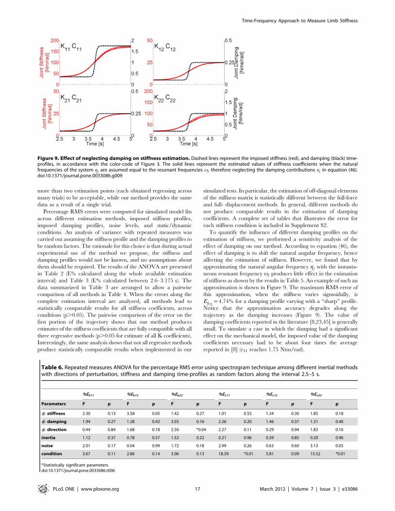
more than two estimation points (each obtained regressing across
many trials) to be acceptable, while our method provides the same
data as a result of a single trial.
Percentage RMS errors were computed for simulated model fits
across different estimation methods, imposed stiffness profiles,
imposed damping profiles, noise levels, and static/dynamic
conditions. An analysis of variance with repeated measures was
carried out assuming the stiffness profile and the damping profiles to
be random factors. The rationale for this choice is that during actual
experimental use of the method we propose, the stiffness and
damping profiles would not be known, and no assumptions about
them should be required. The results of the ANOVA are presented
in Table 2 (E% calculated along the whole available estimation
interval) and Table 3 (E% calculated between 2.6–3.175 s). The
data summarized in Table 3 are arranged to allow a pairwise
comparison of all methods in Table 4. When the errors along the
complete estimation interval are analyzed, all methods lead to
statistically comparable results for all stiffness coefficients, across
conditions (p.0.05). The pairwise comparison of the error on the
first portion of the trajectory shows that our method produces
estimates of the stiffness coefficients that are fully compatible with all
three regressive methods (p.0.05 for estimate of all K coefficients).
Interestingly, the same analysis shows that not all regressive methods
produce statistically comparable results when implemented in our
simulated tests. In particular, the estimation of off-diagonal elements
of the stiffness matrix is statistically different between the full-force
and full- displacement methods. In general, different methods do
not produce comparable results in the estimation of damping
coefficients. A complete set of tables that illustrates the error for
each stiffness condition is included in Supplement S2.
To quantify the influence of different damping profiles on the
estimation of stiffness, we performed a sensitivity analysis of the
effect of damping on our method. According to equation (46), the
effect of damping is to shift the natural angular frequency, hence
affecting the estimation of stiffness. However, we found that by
approximating the natural angular frequency gj with the instanta-
neous resonant frequency vj produces little effect in the estimation
of stiffness as shown by the results in Table 5. An example of such an
approximation is shown in Figure 9. The maximum RMS error of
this approximation, when the stiffness varies sigmoidally, is
Ek22~4.74% for a damping profile varying with a ‘‘sharp’’ profile.
Notice that the approximation accuracy degrades along the
trajectory as the damping increases (Figure 9). The value of
damping coefficients reported in the literature [8,23,45] is generally
small. To simulate a case in which the damping had a significant
effect on the mechanical model, the imposed value of the damping
coefficients necessary had to be about four times the average
reported in [8] (c11 reaches 1.75 Nms/rad).
Table 6. Repeated measures ANOVA for the percentage RMS error using spectrogram technique among different inertial methodswith directions of perturbation, stiffness and damping time-profiles as random factors along the interval 2.5–5 s.
%Ek11 %Ek12 %Ek22 %Ec11 %Ec12 %Ec22
Parameters F p F p F p F p F p F p
# stiffness 2.30 0.13 3.58 0.05 1.42 0.27 1.01 0.55 1.34 0.30 1.85 0.18
# damping 1.94 0.27 1.28 0.42 3.03 0.16 2.26 0.20 1.46 0.37 1.31 0.40
# direction 0.44 0.84 1.68 0.18 2.50 *0.04 2.27 0.11 0.29 0.94 1.83 0.16
inertia 1.12 0.37 0.78 0.57 1.52 0.22 0.21 0.96 0.39 0.85 0.20 0.96
noise 2.01 0.17 0.04 0.99 1.72 0.18 2.99 0.26 0.63 0.60 3.13 0.05
condition 3.67 0.11 2.86 0.14 3.06 0.13 18.39 *0.01 5.81 0.09 15.52 *0.01
*Statistically significant parameters.doi:10.1371/journal.pone.0033086.t006
Figure 9. Effect of neglecting damping on stiffness estimation. Dashed lines represent the imposed stiffness (red), and damping (black) time-profiles, in accordance with the color-code of Figure 3. The solid lines represent the estimated values of stiffness coefficients when the naturalfrequencies of the system gj are assumed equal to the resonant frequencies vj therefore neglecting the damping contributions aj in equation (46).doi:10.1371/journal.pone.0033086.g009
Time-Frequency Approach to Measure Limb Stiffness
PLoS ONE | www.plosone.org 17 March 2012 | Volume 7 | Issue 3 | e33086
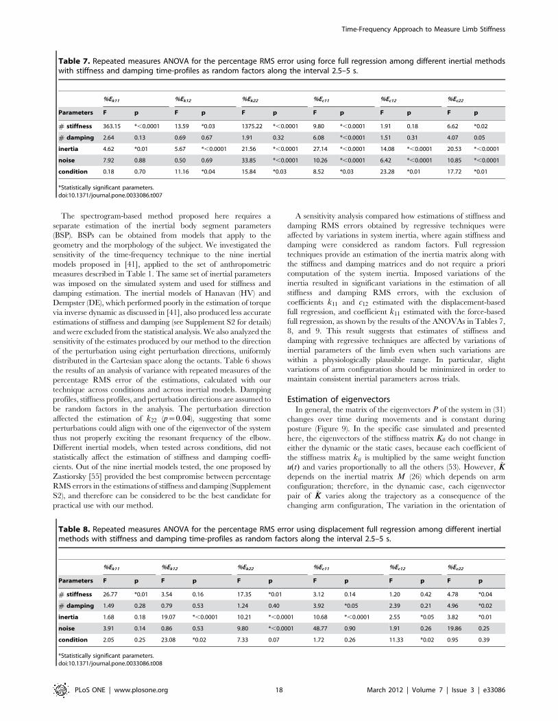
The spectrogram-based method proposed here requires a
separate estimation of the inertial body segment parameters
(BSP). BSPs can be obtained from models that apply to the
geometry and the morphology of the subject. We investigated the
sensitivity of the time-frequency technique to the nine inertial
models proposed in [41], applied to the set of anthropometric
measures described in Table 1. The same set of inertial parameters
was imposed on the simulated system and used for stiffness and
damping estimation. The inertial models of Hanavan (HV) and
Dempster (DE), which performed poorly in the estimation of torque
via inverse dynamic as discussed in [41], also produced less accurate
estimations of stiffness and damping (see Supplement S2 for details)
and were excluded from the statistical analysis. We also analyzed the
sensitivity of the estimates produced by our method to the direction
of the perturbation using eight perturbation directions, uniformly
distributed in the Cartesian space along the octants. Table 6 shows
the results of an analysis of variance with repeated measures of the
percentage RMS error of the estimations, calculated with our
technique across conditions and across inertial models. Damping
profiles, stiffness profiles, and perturbation directions are assumed to
be random factors in the analysis. The perturbation direction
affected the estimation of k22 (p~0:04), suggesting that some
perturbations could align with one of the eigenvector of the system
thus not properly exciting the resonant frequency of the elbow.
Different inertial models, when tested across conditions, did not
statistically affect the estimation of stiffness and damping coeffi-
cients. Out of the nine inertial models tested, the one proposed by
Zastiorsky [55] provided the best compromise between percentage
RMS errors in the estimations of stiffness and damping (Supplement
S2), and therefore can be considered to be the best candidate for
practical use with our method.
A sensitivity analysis compared how estimations of stiffness and
damping RMS errors obtained by regressive techniques were
affected by variations in system inertia, where again stiffness and
damping were considered as random factors. Full regression
techniques provide an estimation of the inertia matrix along with
the stiffness and damping matrices and do not require a priori
computation of the system inertia. Imposed variations of the
inertia resulted in significant variations in the estimation of all
stiffness and damping RMS errors, with the exclusion of
coefficients k11 and c12 estimated with the displacement-based
full regression, and coefficient k11 estimated with the force-based
full regression, as shown by the results of the ANOVAs in Tables 7,
8, and 9. This result suggests that estimates of stiffness and
damping with regressive techniques are affected by variations of
inertial parameters of the limb even when such variations are
within a physiologically plausible range. In particular, slight
variations of arm configuration should be minimized in order to
maintain consistent inertial parameters across trials.
Estimation of eigenvectorsIn general, the matrix of the eigenvectors P of the system in (31)
changes over time during movements and is constant during
posture (Figure 9). In the specific case simulated and presented
here, the eigenvectors of the stiffness matrix Kh do not change in
either the dynamic or the static cases, because each coefficient of
the stiffness matrix kij is multiplied by the same weight function
u(t) and varies proportionally to all the others (53). However, ~KKdepends on the inertial matrix M (26) which depends on arm
configuration; therefore, in the dynamic case, each eigenvector
pair of ~KK varies along the trajectory as a consequence of the
changing arm configuration, The variation in the orientation of
Table 7. Repeated measures ANOVA for the percentage RMS error using force full regression among different inertial methodswith stiffness and damping time-profiles as random factors along the interval 2.5–5 s.
%Ek11 %Ek12 %Ek22 %Ec11 %Ec12 %Ec22
Parameters F p F p F p F p F p F p
# stiffness 363.15 *,0.0001 13.59 *0.03 1375.22 *,0.0001 9.80 *,0.0001 1.91 0.18 6.62 *0.02
# damping 2.64 0.13 0.69 0.67 1.91 0.32 6.08 *,0.0001 1.51 0.31 4.07 0.05
inertia 4.62 *0.01 5.67 *,0.0001 21.56 *,0.0001 27.14 *,0.0001 14.08 *,0.0001 20.53 *,0.0001
noise 7.92 0.88 0.50 0.69 33.85 *,0.0001 10.26 *,0.0001 6.42 *,0.0001 10.85 *,0.0001
condition 0.18 0.70 11.16 *0.04 15.84 *0.03 8.52 *0.03 23.28 *0.01 17.72 *0.01
*Statistically significant parameters.doi:10.1371/journal.pone.0033086.t007
Table 8. Repeated measures ANOVA for the percentage RMS error using displacement full regression among different inertialmethods with stiffness and damping time-profiles as random factors along the interval 2.5–5 s.
%Ek11 %Ek12 %Ek22 %Ec11 %Ec12 %Ec22
Parameters F p F p F p F p F p F p
# stiffness 26.77 *0.01 3.54 0.16 17.35 *0.01 3.12 0.14 1.20 0.42 4.78 *0.04
# damping 1.49 0.28 0.79 0.53 1.24 0.40 3.92 *0.05 2.39 0.21 4.96 *0.02
inertia 1.68 0.18 19.07 *,0.0001 10.21 *,0.0001 10.68 *,0.0001 2.55 *0.05 3.82 *0.01
noise 3.91 0.14 0.86 0.53 9.80 *,0.0001 48.77 0.90 1.91 0.26 19.86 0.25
condition 2.05 0.25 23.08 *0.02 7.33 0.07 1.72 0.26 11.33 *0.02 0.95 0.39
*Statistically significant parameters.doi:10.1371/journal.pone.0033086.t008
Time-Frequency Approach to Measure Limb Stiffness
PLoS ONE | www.plosone.org 18 March 2012 | Volume 7 | Issue 3 | e33086
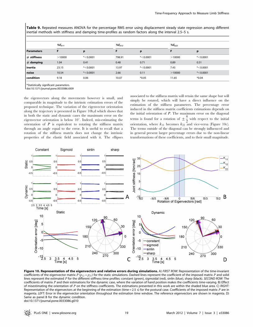
the eigenvectors along the movements however is small, and
comparable in magnitude to the intrinsic estimation errors of the
proposed technique. The variation of the eigenvector orientation
along the trajectory is presented in Figure 10b,d which shows that
in both the static and dynamic cases the maximum error on the
eigenvector orientation is below 10u. Indeed, mis-estimating the
orientation of P is equivalent to rotating the stiffness matrix
through an angle equal to the error. It is useful to recall that a
rotation of the stiffness matrix does not change the intrinsic
properties of the elastic field associated with it. The ellipses
associated to the stiffness matrix will retain the same shape but will
simply be rotated, which will have a direct influence on the
estimation of the stiffness parameters. The percentage error
induced in the stiffness matrix coefficients estimations depends on
the initial orientation of P. The maximum error on the diagonal
terms is found for a rotation of +p
2with respect to the initial
orientation, where k11 becomes k22 and vice-versa (Figure 10c).
The terms outside of the diagonal can be strongly influenced and
in general present larger percentage errors due to the non-linear
transformations of these coefficients, and to their small magnitude.
Figure 10. Representation of the eigenvectors and relative errors during simulations. A) FIRST ROW: Representation of the time-invariantcoefficients of the eigenvector matrix P (p12~p21) for the static simulations. Dashed lines represent the coefficient of the imposed matrix P and solidlines represent the estimated P for the different stiffness time profiles: constant (green), sigmoidal (red), sinlin (blue), sharp (black). SECOND ROW: Thecoefficients of matrix P and their estimations for the dynamic case, where the variation of hand position makes the coefficients time-varying. B) Effectof misestimating the orientation of P on the stiffness coefficients. The estimations presented in this work are within the shaded blue area. C) RIGHT:Representation of the eigenvectors at the beginning of the estimation (time = 2.5 s) for the postural case. Coefficients of the imposed matrix P are inmagenta. LEFT: Error in the eigenvector orientation throughout the estimation time window. The reference eigenvectors are shown in magenta. D)Same as panel B for the dynamic condition.doi:10.1371/journal.pone.0033086.g010
Table 9. Repeated measures ANOVA for the percentage RMS error using displacement steady state regression among differentinertial methods with stiffness and damping time-profiles as random factors along the interval 2.5–5 s.
%Ek11 %Ek12 %Ek22
Parameters F p F p F p
# stiffness .10000 *,0.0001 798.91 *,0.0001 .10000 *,0.0001
# damping 1.04 0.41 0.48 0.71 0.89 0.51
inertia 23.15 *,0.0001 13.97 *,0.0001 7.43 *,0.0001
noise 10.54 *,0.0001 2.66 0.11 .10000 *,0.0001
condition 9.18 0.06 10.07 *0.05 11.65 *0.04
*Statistically significant parameters.doi:10.1371/journal.pone.0033086.t009
Time-Frequency Approach to Measure Limb Stiffness
PLoS ONE | www.plosone.org 19 March 2012 | Volume 7 | Issue 3 | e33086
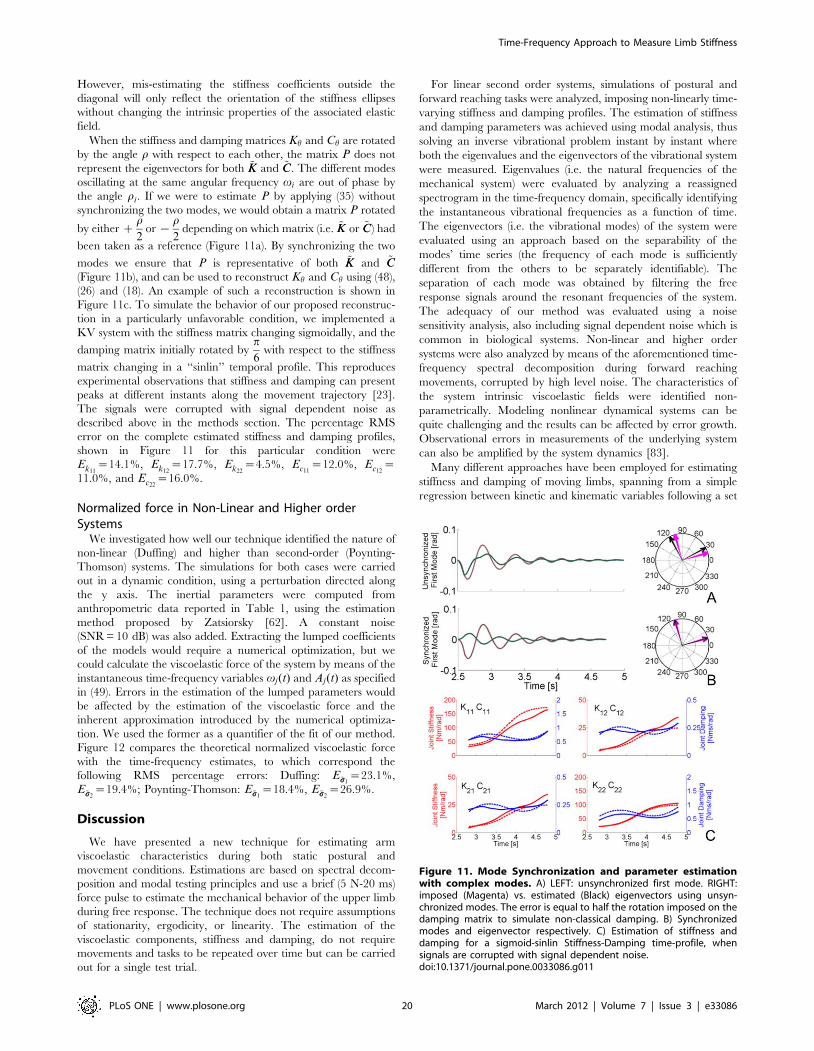
However, mis-estimating the stiffness coefficients outside the
diagonal will only reflect the orientation of the stiffness ellipses
without changing the intrinsic properties of the associated elastic
field.
When the stiffness and damping matrices Kh and Ch are rotated
by the angle r with respect to each other, the matrix P does not
represent the eigenvectors for both ~KK and ~CC. The different modes
oscillating at the same angular frequency vi are out of phase by
the angle ri. If we were to estimate P by applying (35) without
synchronizing the two modes, we would obtain a matrix P rotated
by either zr
2or {
r
2depending on which matrix (i.e. ~KK or ~CC) had
been taken as a reference (Figure 11a). By synchronizing the two
modes we ensure that P is representative of both ~KK and ~CC(Figure 11b), and can be used to reconstruct Kh and Ch using (48),
(26) and (18). An example of such a reconstruction is shown in
Figure 11c. To simulate the behavior of our proposed reconstruc-
tion in a particularly unfavorable condition, we implemented a
KV system with the stiffness matrix changing sigmoidally, and the
damping matrix initially rotated byp
6with respect to the stiffness
matrix changing in a ‘‘sinlin’’ temporal profile. This reproduces
experimental observations that stiffness and damping can present
peaks at different instants along the movement trajectory [23].
The signals were corrupted with signal dependent noise as
described above in the methods section. The percentage RMS
error on the complete estimated stiffness and damping profiles,
shown in Figure 11 for this particular condition were
Ek11~14.1%, Ek12
~17.7%, Ek22~4.5%, Ec11
~12.0%, Ec12~
11.0%, and Ec22~16.0%.
Normalized force in Non-Linear and Higher orderSystems
We investigated how well our technique identified the nature of
non-linear (Duffing) and higher than second-order (Poynting-
Thomson) systems. The simulations for both cases were carried
out in a dynamic condition, using a perturbation directed along
the y axis. The inertial parameters were computed from
anthropometric data reported in Table 1, using the estimation
method proposed by Zatsiorsky [62]. A constant noise
(SNR = 10 dB) was also added. Extracting the lumped coefficients
of the models would require a numerical optimization, but we
could calculate the viscoelastic force of the system by means of the
instantaneous time-frequency variables vj(t) and Aj(t) as specified
in (49). Errors in the estimation of the lumped parameters would
be affected by the estimation of the viscoelastic force and the
inherent approximation introduced by the numerical optimiza-
tion. We used the former as a quantifier of the fit of our method.
Figure 12 compares the theoretical normalized viscoelastic force
with the time-frequency estimates, to which correspond the
following RMS percentage errors: Duffing: E~ss1~23.1%,
E~ss2~19.4%; Poynting-Thomson: E~ss1
~18.4%, E~ss2~26.9%.
Discussion
We have presented a new technique for estimating arm
viscoelastic characteristics during both static postural and
movement conditions. Estimations are based on spectral decom-
position and modal testing principles and use a brief (5 N-20 ms)
force pulse to estimate the mechanical behavior of the upper limb
during free response. The technique does not require assumptions
of stationarity, ergodicity, or linearity. The estimation of the
viscoelastic components, stiffness and damping, do not require
movements and tasks to be repeated over time but can be carried
out for a single test trial.
For linear second order systems, simulations of postural and
forward reaching tasks were analyzed, imposing non-linearly time-
varying stiffness and damping profiles. The estimation of stiffness
and damping parameters was achieved using modal analysis, thus
solving an inverse vibrational problem instant by instant where
both the eigenvalues and the eigenvectors of the vibrational system
were measured. Eigenvalues (i.e. the natural frequencies of the
mechanical system) were evaluated by analyzing a reassigned
spectrogram in the time-frequency domain, specifically identifying
the instantaneous vibrational frequencies as a function of time.
The eigenvectors (i.e. the vibrational modes) of the system were
evaluated using an approach based on the separability of the
modes’ time series (the frequency of each mode is sufficiently
different from the others to be separately identifiable). The
separation of each mode was obtained by filtering the free
response signals around the resonant frequencies of the system.
The adequacy of our method was evaluated using a noise
sensitivity analysis, also including signal dependent noise which is
common in biological systems. Non-linear and higher order
systems were also analyzed by means of the aforementioned time-
frequency spectral decomposition during forward reaching
movements, corrupted by high level noise. The characteristics of
the system intrinsic viscoelastic fields were identified non-
parametrically. Modeling nonlinear dynamical systems can be
quite challenging and the results can be affected by error growth.
Observational errors in measurements of the underlying system
can also be amplified by the system dynamics [83].
Many different approaches have been employed for estimating
stiffness and damping of moving limbs, spanning from a simple
regression between kinetic and kinematic variables following a set
Figure 11. Mode Synchronization and parameter estimationwith complex modes. A) LEFT: unsynchronized first mode. RIGHT:imposed (Magenta) vs. estimated (Black) eigenvectors using unsyn-chronized modes. The error is equal to half the rotation imposed on thedamping matrix to simulate non-classical damping. B) Synchronizedmodes and eigenvector respectively. C) Estimation of stiffness anddamping for a sigmoid-sinlin Stiffness-Damping time-profile, whensignals are corrupted with signal dependent noise.doi:10.1371/journal.pone.0033086.g011
Time-Frequency Approach to Measure Limb Stiffness
PLoS ONE | www.plosone.org 20 March 2012 | Volume 7 | Issue 3 | e33086
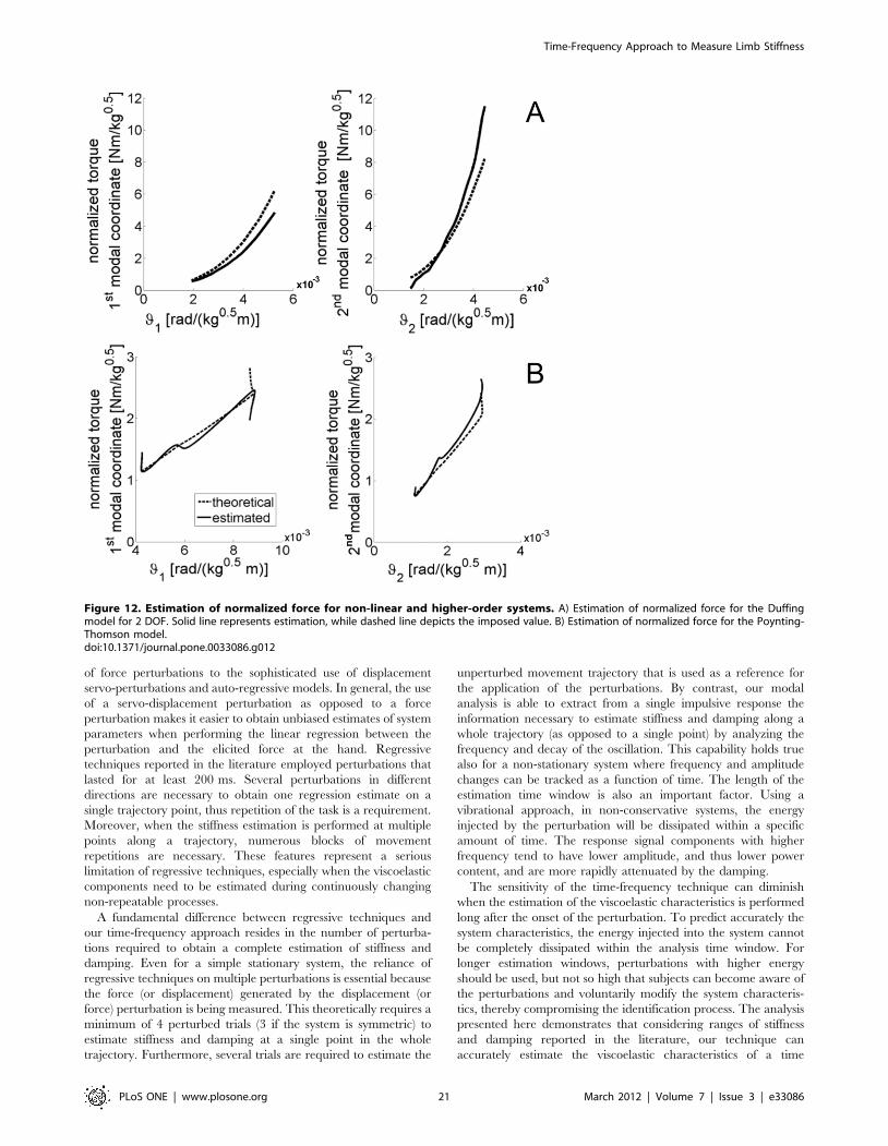
of force perturbations to the sophisticated use of displacement
servo-perturbations and auto-regressive models. In general, the use
of a servo-displacement perturbation as opposed to a force
perturbation makes it easier to obtain unbiased estimates of system
parameters when performing the linear regression between the
perturbation and the elicited force at the hand. Regressive
techniques reported in the literature employed perturbations that
lasted for at least 200 ms. Several perturbations in different
directions are necessary to obtain one regression estimate on a
single trajectory point, thus repetition of the task is a requirement.
Moreover, when the stiffness estimation is performed at multiple
points along a trajectory, numerous blocks of movement
repetitions are necessary. These features represent a serious
limitation of regressive techniques, especially when the viscoelastic
components need to be estimated during continuously changing
non-repeatable processes.
A fundamental difference between regressive techniques and
our time-frequency approach resides in the number of perturba-
tions required to obtain a complete estimation of stiffness and
damping. Even for a simple stationary system, the reliance of
regressive techniques on multiple perturbations is essential because
the force (or displacement) generated by the displacement (or
force) perturbation is being measured. This theoretically requires a
minimum of 4 perturbed trials (3 if the system is symmetric) to
estimate stiffness and damping at a single point in the whole
trajectory. Furthermore, several trials are required to estimate the
unperturbed movement trajectory that is used as a reference for
the application of the perturbations. By contrast, our modal
analysis is able to extract from a single impulsive response the
information necessary to estimate stiffness and damping along a
whole trajectory (as opposed to a single point) by analyzing the
frequency and decay of the oscillation. This capability holds true
also for a non-stationary system where frequency and amplitude
changes can be tracked as a function of time. The length of the
estimation time window is also an important factor. Using a
vibrational approach, in non-conservative systems, the energy
injected by the perturbation will be dissipated within a specific
amount of time. The response signal components with higher
frequency tend to have lower amplitude, and thus lower power
content, and are more rapidly attenuated by the damping.
The sensitivity of the time-frequency technique can diminish
when the estimation of the viscoelastic characteristics is performed
long after the onset of the perturbation. To predict accurately the
system characteristics, the energy injected into the system cannot
be completely dissipated within the analysis time window. For
longer estimation windows, perturbations with higher energy
should be used, but not so high that subjects can become aware of
the perturbations and voluntarily modify the system characteris-
tics, thereby compromising the identification process. The analysis
presented here demonstrates that considering ranges of stiffness
and damping reported in the literature, our technique can
accurately estimate the viscoelastic characteristics of a time
Figure 12. Estimation of normalized force for non-linear and higher-order systems. A) Estimation of normalized force for the Duffingmodel for 2 DOF. Solid line represents estimation, while dashed line depicts the imposed value. B) Estimation of normalized force for the Poynting-Thomson model.doi:10.1371/journal.pone.0033086.g012
Time-Frequency Approach to Measure Limb Stiffness
PLoS ONE | www.plosone.org 21 March 2012 | Volume 7 | Issue 3 | e33086
varying coupled linear system well beyond 2 s after the onset of the
perturbation.
Tracking stiffness and damping changes using regressive
techniques requires multiple perturbations at different instants.
This is particularly critical when trying to identify a system with
fast dynamics and sudden changes in stiffness and damping. The
Nyquist–Shannon sampling theorem specifies that to identify a
change in a viscoelastic variable occurring at a frequency fk, the
time gap between the points at which the variable is to be
identified must be smaller than the Nyquist period tNk ~
1
2fk
. By
contrast, our technique does not require multiple perturbations to
identify fast changing dynamics of the viscoelastic field and is able
to track fast dynamic changes such as the ‘‘sharp’’ presented here.
Estimation accuracy does tend to degrade as the changes in
stiffness and damping become faster because of the filtering effect
of the spectrogram, when several sliding windows are averaged
together.
Arm stiffness can be influenced by three separate factors: the
intrinsic stiffness of muscles and tendons, the level of voluntary co-
contraction, and the intervention of reflexes. Our technique’s
capacity for continuous stiffness estimation following a perturba-
tion duration of only 20 ms separates these three components
because they tend to predominate in different epochs of a
movement. For example, we can observe the influences of each
factor as the estimated stiffness changes in time: the intrinsic
stiffness is mostly dependent upon the biomechanics of the limb
which will influence the stiffness estimation right after the
perturbation is applied; stretch sensitive reflexes, usually act on a
specific time scale between 70 and 150 ms after the perturbation
onset, and their effects are visible on the stiffness estimation with a
50 ms delay [14,84]. This temporal segmentation implies that
whatever is estimated more than 200 ms after the perturbation
onset may be influenced by voluntary control. Hence, by
analyzing how stiffness evolves in time, the effect of each control
loop can be studied in single trials. The rapidity of this estimation
is thus suitable for identifying stiffness time-profiles during
movement adaptation paradigms, thereby providing a fundamen-
tal tool to identify motor control strategies. The capacity to
monitor variations in stiffness and damping during single trials
may particularly benefit the study of rehabilitation training.
During robotic therapy, an assistive force field is applied to the
limbs of impaired individuals to supply the minimal amount of
force necessary to assist them in completing motor tasks. The force
is then diminished on a trial-by-trial basis to help the subject
regain independence. During such a procedure, the modulation of
the assistive force field is different from trial to trial (i.e. non-
repeatable motor tasks) and a low fatigue threshold may limit the
number of trials the subject can perform [85,86,87,88]. The
robotic manipulandum can be a viable tool to estimate limb
stiffness, but its utility has so far been restricted by the limitations
of regressive techniques. Our proposed approach avoids these
limitations.
The technique we propose also has applications in the study of
motor adaptation to novel environments where constant, velocity-,
and acceleration-dependent force fields are present [89,90,91].
The object of analysis often is to capture stiffness and other
characteristics in individual perturbed movements, such as the
initial perturbed movement or single catch trials. Our approach
also applies to cases where a subject adapts to an inertial force field
delivered without mechanical contact at the arm [90], because the
perturbations needed for modal time-frequency analysis are
introduced without robotic devices. The modal analysis techniques
can be applied on a trial-by-trial basis to monitor how stiffness
varies during motor adaptation.
Supporting Information
Supplement S1 Stiffness and Damping Asymmetry dueto Dynamic effects. The asymmetry of the dynamic matrix
LH h, _hh� �
_hh
Lh, which is a component of the joint stiffness KKh, is
analyzed.
(PDF)
Supplement S2 Tables of estimation methods statisticalcomparison. Tables showing the Stiffness and Damping RMS
percentage errors of all estimation methods for KV models during
posture and movements. Errors are computed both along the
entire stiffness profile and between the first two estimation points
used with the regressive methods. The influence of different
inertial models for the case sigmoid-sinlin-SDN (K-C-noise), is also
shown.
(PDF)
Supplement S3 Third order form of the PT model andconditions for oscillatory free response. Analysis of the
third-order PT model’s oscillatory behavior: a limited region of
non-oscillatory free response exists for a ratio between the stiffness
of the tendon and the stiffness of the muscle fibers greater than
eight.
(PDF)
Supplement S4 Dynamics zero of the PT model impulseresponse. An analytical demonstration on the presence of a
dynamic zero for the third order PT model.
(PDF)
Acknowledgments
The authors thank Dr. Sandro Mussa-Ivaldi and the members of the
Robotics Lab at Northwestern University for their support. We are grateful
to Dr. Eric Perreault for his useful suggestions that enabled us to clarify
several concepts in the paper.
Author Contributions
Conceived and designed the experiments: DP. Performed the experiments:
DP AP. Analyzed the data: DP. Contributed reagents/materials/analysis
tools: DP AP PD JRL. Wrote the paper: DP AP PD JRL.
References
1. de Vlugt E, Schouten AC, van der Helm FCT (2003) Closed-loop multivariable
system identification for the characterization of the dynamic arm compliance
using continuous force disturbances: a model study. Journal of neuroscience
methods 122: 123–140.
2. Palazzolo JJ, Ferraro M, Krebs HI, Lynch D, Volpe BT, et al. (2007) Stochastic
estimation of arm mechanical impedance during robotic stroke rehabilitation.
IEEE transactions on neural systems and rehabilitation engineering : a publication
of the IEEE Engineering in Medicine and Biology Society 15: 94–103.
3. Perreault EJ, Kirsch RF, Acosta AM (1999) Multiple-input, multiple-output
system identification for characterization of limb stiffness dynamics. Biological
cybernetics 80: 327–337.
4. Perreault EJ, Kirsch RF, Crago PE (2001) Effects of voluntary force generation
on the elastic components of endpoint stiffness. Experimental Brain Research
141: 312–323.
5. Perreault EJ, Kirsch RF, Crago PE (2004) Multijoint dynamics and postural
stability of the human arm. Experimental Brain Research 157: 507–517.
Time-Frequency Approach to Measure Limb Stiffness
PLoS ONE | www.plosone.org 22 March 2012 | Volume 7 | Issue 3 | e33086
6. Dolan JM, Friedman MB, Nagurka ML (1993) Dynamic and loaded impedancecomponents in the maintenance of human arm posture. IEEE Transactions on
Systems, Man, and Cybernetics 23: 698–709.
7. Mussa-Ivaldi FA, Hogan N, Bizzi E (1985) Neural, mechanical, and geometric
factors subserving arm posture in humans. Journal of Neuroscience 5:2732–2732.
8. Tsuji T, Morasso PG, Goto K, Ito K (1995) Human hand impedance
characteristics during maintained posture. Biological cybernetics 72: 475–485.
9. Darainy M, Malfait N, Gribble PL, Towhidkhah F, Ostry DJ (2004) Learning to
control arm stiffness under static conditions. Journal of neurophysiology 92:3344–3344.
10. Franklin DW, Milner TE (2003) Adaptive control of stiffness to stabilize handposition with large loads. Experimental Brain Research 152: 211–220.
11. Burdet E, Osu R, Franklin DW, Yoshioka T, Milner TE, et al. (2000) A methodfor measuring endpoint stiffness during multi-joint arm movements. Journal of
biomechanics 33: 1705–1709.
12. Franklin DW, Burdet E, Osu R, Kawato M, Milner TE (2003) Functional
significance of stiffness in adaptation of multijoint arm movements to stable andunstable dynamics. Experimental brain research 151: 145–157.
13. Franklin DW, Liaw G, Milner TE, Osu R, Burdet E, et al. (2007) Endpointstiffness of the arm is directionally tuned to instability in the environment.
Journal of Neuroscience 27: 7705–7705.
14. Frolov AA, Prokopenko RA, Dufosse M, Ouezdou FB (2006) Adjustment of thehuman arm viscoelastic properties to the direction of reaching. Biological
cybernetics 94: 97–109.
15. Gomi H, Kawato M (1997) Human arm stiffness and equilibrium-point
trajectory during multi-joint movement. Biological Cybernetics 76: 163–171.
16. Mah CD (2001) Spatial and temporal modulation of joint stiffness during
multijoint movement. Experimental Brain Research. pp 492–506.
17. Darainy M, Towhidkhah F, Ostry DJ (2007) Control of hand impedance under
static conditions and during reaching movement. Journal of neurophysiology 97:2676–2685.
18. Wong J, Wilson ET, Malfait N, Gribble PL (2009) Limb stiffness is modulatedwith spatial accuracy requirements during movement in the absence of
destabilizing forces. Journal of neurophysiology 101: 1542–1549.
19. Wong J, Wilson ET, Malfait N, Gribble PL (2009) The influence of visual
perturbations on the neural control of limb stiffness. Journal of neurophysiology
101: 246–257.
20. Kirsch RF, Kearney RE (1997) Identification of time-varying stiffness dynamics
of the human ankle joint during an imposed movement. Experimental brainresearch Experimentelle Hirnforschung Experimentation cerebrale 114: 71–85.
21. Ludvig D, Starret Visser T, Giesbrecht H, Kearney R (2011) Identification ofTime-Varying Intrinsic and Reflex Joint Stiffness. IEEE transactions on bio-
medical engineering.
22. Xu Y, Hollerbach JM (1999) A Robust Ensemble Data Method for
Identification of Human Joint Mechanical Properties During Movement. 46:
409–419.
23. Bennett DJ, Hollerbach JM, Xu Y, Hunter IW (1992) Time-varying stiffness of
human elbow joint during cyclic voluntary movement. Experimental BrainResearch 88: 433–442.
24. Milner TE (1993) Dependence of elbow viscoelastic behavior on speed andloading in voluntary movements. Exp Brain Res 93: 177–180.
25. Stein RB, Kearney RE (1995) Nonlinear behavior of muscle reflexes at thehuman ankle joint. J Neurophysiol 73: 65–72.
26. Franklin DW, Osu R, Burdet E, Kawato M, Milner TE (2003) Adaptation tostable and unstable dynamics achieved by combined impedance control and
inverse dynamics model. Journal of neurophysiology 90: 3270–3282.
27. Ravichandran VJ, Perreault EJ, Westwick DT, Cohen N (2004) Nonparametric
identification of the elbow joint stiffness under compliant loads. Conferenceproceedings : Annual International Conference of the IEEE Engineering in
Medicine and Biology Society IEEE Engineering in Medicine and Biology
Society Conference 7: 4706–4709.
28. Huang NE, Shen SSP (2005) Hilbet-Huang Transform and Its Applications:
World Scientific Publishing Co. Pte. Ltd.
29. Shi ZY, Law SS (2007) Identification of Linear Time-Varying Dynamical
Systems Using Hilbert Transform and Empirical Mode Decomposition Method.Journal of Applied Mechanics 74: 223–223.
30. Shi ZY, Law SS, Xu X (2009) Identification of linear time-varying mdofdynamic systems from forced excitation using Hilbert transform and EMD
method. Journal of Sound and Vibration 321: 572–589.
31. Papandreou-Suppappola A (2003) Applications in time-frequency signal
processing CRC Press.
32. Bortolami SB, DiZio P, Rabin E, Lackner JR (2003) Analysis of human postural
responses to recoverable falls. Experimental brain research 151: 387–404.
33. Padovan J, Guo Y (1988) General response of viscoelastic systems modelled by
fractional operators. Journal of the Franklin Institute 325: 247–275.
34. Tomas-Rodriguez M, Banks SP (2010) Linear, Time-varying Approximations toNonlinear Dynamical Systems with Applications in Control and Optimization.
Berlin: Springer.
35. Galleani L, Cohen L (2004) Direct Time-Frequency Characterization of Linear
Systems Governed by Differential Equations. IEEE Signal Processing Letters 11:721–724.
36. Nelson DJ (2001) Cross-spectral methods for processing speech. The Journal ofthe Acoustical Society of America 110: 2575–2575.
37. Auger F, Flandrin P (1995) Representations by the Reassignment Method. IEEETransactions on Signal Processing 43: 1068–1089.
38. Fulop SA, Fitz K (2006) A spectrogram for the twenty-first century. AcousticsToday 2: 26–33.
39. Fulop SA, Fitz K (2006) Algorithms for computing the time-correctedinstantaneous frequency (reassigned) spectrogram, with applications. The
Journal of the Acoustical Society of America 119: 360–360.
40. Feldman M (2007) Identification of weakly nonlinearities in multiple coupled
oscillators. Journal of Sound and Vibration 303: 357–370.
41. Piovesan D, Pierobon A, DiZio P, Lackner JR (2011) Comparative Analysis of
Methods for Estimating Arm Segment Parameters and Joint Torques FromInverse Dynamics. Journal of Biomechanical Engineering 133: 031003.
42. Hof AL (1998) In vivo measurement of the series elasticity release curve ofhuman triceps surae muscle. Journal of Biomechanics 31: 793–800.
43. Mares T (2008) Curvilinear tensor analysis of an elastic heterogenousepicycloidal thick walled tube. Bulletin of Applied Mechanics 4: 37–47.
44. Braun S (1997) Time–Frequency Characteristics of Non-Linear Systems.Mechanical Systems and Signal Processing 11: 611–620.
45. Popescu F, Hidler JM, Rymer WZ (2003) Elbow impedance during goal-directed movements. Experimental brain research Experimentelle Hirn-
forschung Experimentation cerebrale 152: 17–28.
46. Kistemaker Da, Rozendaal La (2011) In vivo dynamics of the musculoskeletal
system cannot be adequately described using a stiffness-damping-inertia model.PloS one 6: e19568–e19568.
47. Schouten AC, de Vlugt E, van Der Helm FC, Brouwn GG (2001) Optimalposture control of a musculo-skeletal arm model. Biological Cybernetics 84:
143–152.
48. Westwick DT, Perreault EJ (2011) Closed-loop identification: application to the
estimation of limb impedance in a compliant environment. IEEE transactions on
bio-medical engineering 58: 521–530.
49. Flash T, Mussa-Ivaldi F (1990) Human arm stiffness characteristics during the
maintenance of posture. Experimental Brain Research 82: 315–326.
50. Stroeve S (1999) Impedance characteristics of a neuromusculoskeletal model ofthe human arm I. Posture control. Biological Cybernetics 81: 475–494.
51. Lacquaniti F, Carrozzo M, Borghese NA (1993) Time-varying mechanicalbehavior of multijointed arm in man. Journal of Neurophysiology 69:
1443–1443.
52. Kao I, Cutkosky MR, Johansson RS (1997) Robotic stiffness control and
calibration as applied to human grasping tasks. IEEE Transactions on Robotics
and Automation 13: 557–566.
53. Tee KP, Burdet E, Chew CM, Milner TE (2004) A model of force and
impedance in human arm movements. Biological cybernetics 90: 368–375.
54. Lee G (1998) On cross effects of seismic respo ns s of structures. Engineering
Structures 20: 503–509.
55. Ma F, Imam A, Morzfeld M (2009) The decoupling of damped linear systems in
oscillatory free vibration. Journal of Sound and Vibration 324: 408–428.
56. Hanavan EPJ (1964) A mathematical model of the human body. Dayton, Ohio:
Wright-Patterson Air Force Base.
57. Dempster WT (1955) Space requirements of the seated operator. Geometrical,
kinematic, and mechanical aspects of the body with special reference to thelimbs. Dayton, Ohio: Wright Air Development, 159 159.
58. Chandler RF, Clauser CE, McConville JT, Reynolds HM, Young JW (1975)
Investigation of inertial properties of the human body. Dayton, Ohio: Wright-
Patterson Air Force Base.
59. Clauser CE, McConville JT, Young JW (1969) Weight, volume, and center of
mass of segments of the human body. Dayton, Ohio: Wright-Patterson Air ForceBase, 70 70.
60. McConville JT, Churchill TD, Kaleps I, Clauser CE, Cuzzi J (1980)Anthropometric relationships of body and body segment moments of inertia.
Dayton, Ohio: Wright-Patterson Air Force Base.
61. Zatsiorsky V, Seluyanov V (1983) The mass and inertia characteristics of the
main segments of the human body. In: Matsui HaKK, ed. Champaign, Illinois:Human Kinetics. pp 1152–1159.
62. Zatsiorsky VM (2002) Best predictive regression equations for estimting inertialproperties of body segments in males, Appendix A2.8. In: Zatsiorsky VM, ed.
Kinetics of human motion. Champain, IL: Human Kinetics. pp 600–601.
63. de Leva P (1996) Adjustments to Zatsiorsky-Seluyanov’s segment inertia
parameters. Journal of Biomechanics 29: 1223–1230.
64. Angeles J (1992) On the application of Mohr’s circle to 2-dof vibration analysis: a
tutorial. Journal of sound and vibration 154: 556–567.
65. Gohberg I, Lancaster P, Rodman L (2009) Matrix polynomials; O’Malley J, RE,
eds. Philadelphia, PA: SIAM.
66. Lancaster P, Prells U (2005) Inverse problems for damped vibrating systems.
Journal of Sound and Vibration 283: 891–914.
67. Inman DJ, Andry ANJ (1980) Some results on the nature of eigenvalues of
discrete damped linear systems. ASME Journal of Applied Mechanics 47:927–930.
68. Starek L, Inman DJ, Kress A (1992) A Symmetric Inverse Vibration Problem.Journal of Vibration and Acoustics 114: 564–564.
69. Ewins DJ (2000) Modal testing: theory, practice and applications. Baldock,Hertfordshire, England: Research Studies Press LTD.
70. Cohen L, Galleani L, Hedges R, Hughes D (2002) Time-frequency analysis of avariable stiffness model for fault development. Digital Signal 440: 429–440.
Time-Frequency Approach to Measure Limb Stiffness
PLoS ONE | www.plosone.org 23 March 2012 | Volume 7 | Issue 3 | e33086
71. Feldman M (2011) Hilbert transform in vibration analysis. Mechanical Systems
and Signal Processing 25: 735–802.72. Milner TE, Franklin DW (2005) Impedance control and internal model use
during the initial stage of adaptation to novel dynamics in humans. The Journal
of physiology 567: 651–664.73. Popescu FC, Rymer WZ (2000) End points of planar reaching movements are
disrupted by small force pulses: an evaluation of the hypothesis of equifinality.Journal of Neurophysiology 84: 2670–2679.
74. Inman DJ (1989) Vibration: with control, measurement, and stability. Engle-
wood Cliffs, NJ: Prentice Hall.75. Press WH, Flannery BP, Teukolsky SA, Vetterling WT (1992) Numerical
Recipes in C: The Art of Scientific Computing Cambridge University Press.76. Mitrovic D, Klanke S, Osu R, Kawato M, Vijayakumar S (2010) A
computational model of limb impedance control based on principles of internalmodel uncertainty. PloS one 5: e13601–e13601.
77. Tresch MC, Cheung VCK, d’Avella A (2006) Matrix factorization algorithms
for the identification of muscle synergies: evaluation on simulated andexperimental data sets. Journal of Neurophysiology 95: 2199–2212.
78. Beek PJ, Schmidt RC, Morris AW, Sim MY, Turvey MT (1995) Linear andnonlinear stiffness and friction in biological rhythmic movements. Biological
Cybernetics 73: 499–507.
79. Schultz AB, Faulkner JA, Kadhiresan VA (1991) A simple Hill element-nonlinear spring model of muscle contraction biomechanics. Journal of applied
physiology (Bethesda, Md : 1985) 70: 803–812.80. Silva P, Moreno M, Mancini M, Fonseca S, Turvey MT (2007) Steady-state
stress at one hand magnifies the amplitude, stiffness, and non-linearity ofoscillatory behavior at the other hand. Neuroscience letters 429: 64–68.
81. Sup F, Bohara A, Goldfarb M (2008) Design and control of a powered
transfemoral prosthesis. The International Journal of Robotics Research 27:263–263.
82. Piovesan D, Dizio P, Lackner JR (2009) A new time-frequency approach toestimate single joint upper limb impedance. Engineering in Medicine and
Biology Society (EMBS): Annual International Conference of the IEEE 1:
1282–1285.
83. Orrell D (2005) Estimating error growth and shadow behavior in nonlinear
dynamical systems. International journal of bifurcation and chaos in applied
sciences and engineering 15: 3265–3265.
84. Frolov aa, Dufosse M, Rızek S, Kaladjian a (2000) On the possibility of linear
modelling the human arm neuromuscular apparatus. Biological cybernetics 82:
499–515.
85. Casadio M, Giannoni P, Masia L, Morasso P, Sandini G, et al. (2009) Robot
therapy of the upper limb in stroke patients: preliminary experiences for the
principle-based use of this technology. Funct Neurol 24: 195–202.
86. Casadio M, Giannoni P, Morasso P, Sanguineti V (2009) A proof of concept
study for the integration of robot therapy with physiotherapy in the treatment of
stroke patients. Clinical rehabilitation 23: 217–228.
87. Piovesan D, Casadio M, Morasso P, Giannoni P (2011) Influence of Visual
Feedback in the Regulation of Arm Stiffness Following Stroke. Engineering in
Medicine and Biology Society (EMBS): Annual International Conference of the
IEEE. pp 8239–8242.
88. Piovesan D, Casadio M, Mussa-Ivaldi FA, Morasso PG (2011) Multijoint arm
stiffness during movements following stroke: Implications for robot therapy.
Rehabilitation Robotics (ICORR), 2011 IEEE International Conference on. pp
1–7.
89. Kolesnikov M, Piovesan D, Lynch K, Mussa-Ivaldi F (2011) On Force
Regulation Strategies in Predictable Environments. Engineering in Medicine
and Biology Society (EMBS): Annual International Conference of the IEEE 1:
4076–4081.
90. Lackner JR, Dizio P (1994) Rapid adaptation to Coriolis force perturbations of
arm trajectory. Journal of Neurophysiology 72: 299–313.
91. Shadmehr R, Mussa-Ivaldi F (1994) Adaptive representation of dynamics during
learning of a motor task. The Journal of Neuroscience 14: 3208–3224.
Time-Frequency Approach to Measure Limb Stiffness
PLoS ONE | www.plosone.org 24 March 2012 | Volume 7 | Issue 3 | e33086
Recommended