Measuring Financial Integration in New EU Member

States

Markus Baltzer, Lorenzo Cappiello, Roberto A. De Santis, and Simone Manganelli∗†

December 2007

∗Cappiello, De Santis and Manganelli are with the European Central Bank, Kaiserstrasse 29,

60311 Frankfurt am Main, Germany. Email: lorenzo.cappiello@ecb.int, tel: +49-69 1344 8765;

roberto.de_santis@ecb.int, tel: +49-69 1344 6611; simone.manganelli@ecb.int, tel: +49-69 1344 7347.

Baltzer is with Deutsche Bundesbank, email: markus.baltzer@bundesbank.de, tel: +49 69 9566 8473.†We thank Philipp Hartmann for valuable comments. Of course, remaining errors are ours alone.

This paper is forthcoming as an ECB Occasional Paper. The views expressed in this paper are those

of the authors and do not necessarily reflect those of the European Central Bank, the Deutsche

Bundesbank or the Eurosystem.

1

Executive SummaryIn light of the recent accession of new countries in the European Union (EU) and

their future entry in the euro area, it has become increasingly important to follow

developments in these markets. This study provides a comprehensive overview on the

state of financial integration in the new EU Member States. These countries comprise

the Czech Republic, Estonia, Hungary, Latvia, Lituania, Poland, and Slovakia, which

joined the EU on 1 May 2004, and Romania and Bulgaria, which joined on 1 January

2007. Since the bulk of the analysis covers the period from 1996 until 2006, we also

consider EU member states, Slovenia (which joined the euro area on 1 January 2007),

as well as Cyprus and Malta (which joined on 1 January 2008).

Monitoring these countries’ economies is not only relevant from a policy-making

point of view, but is also interesting in itself owing to their specific characteristics.

For instance, on the real economy side, many of these countries went from being

centrally planned economies, through market economies, to fully open economies,

taking about twelve years to become members of a free trade area. Moreover, these

economies experienced very rapid development and liberalisation of their financial

markets undergoing these changes at roughly the same pace. Finally, since the new

EU Member States will eventually join the euro area, it is important to monitor

developments in their financial markets as well as links with the euro area from a

monetary policy perspective.

To assess the degree of financial integration of the new EU Member States (plus

Cyprus, Malta and Slovenia), this paper adopts a methodology developed previously

by Baele et al. (2004). Subject to data availability, this paper replicates the indicators

used in that study. This allows us to build on an already established methodology

and, at the same time, directly compare developments in the new EU Member States

(plus Cyprus, Malta and Slovenia) with those in the euro area. Some of the results we

obtain need to be interpreted with caution due the lower quality of some data for the

countries included in the analysis. However, after the entry in the European Union,

the availability and reliability of data has been gradually improving.

The study considers three broad categories of financial integration measures: (i)

price-based, which capture discrepancies in asset prices across different national mar-

kets; (ii) news-based, which analyse the impact that common factors have on the

return process of an asset; (iii) quantity-based, which aim at quantifying the effects

of frictions on the demand for and supply of securities.

This paper finds that financial markets in the new EU Member States (plus

Cyprus, Malta and Slovenia) are significantly less integrated than those of the euro

area. Nevertheless, there is strong evidence that the process of integration is well

2

under way and has accelerated since accession to the EU.

According to the indicators adopted in the paper, money and banking markets are

becoming increasingly integrated both among themselves and vis-à-vis the euro area.

However, it should be noticed that the process of financial integration in the new

EU Member States (plus Cyprus, Malta and Slovenia) is probably driven by different

factors than those behind the euro area. The transition from planned to market

economies has led to rapid financial developments, which has been further boosted

by a strong foreign, mainly EU, banking presence. For instance, the percentage of

asset shares of foreign-owned banks (relative to total bank sector assets) increased

from 30% in 1997 to around 75% in 2005.

As for government bond markets, only the largest economies (the Czech Republic,

Poland and to a lesser extent Hungary) exhibit signs of integration. These results need

to be interpreted with caution, as the liquidity of the underlying markets may distort

the measures.

Finally, the evidence for equities suggest a relatively low level of integration. How-

ever, we find that stock markets are increasingly affected by euro area shocks, espe-

cially after the accession date (May 2004).

3

1 Introduction

Developments in financial markets have shaped the economic and policy debate in

recent years. Financial integration issues have played an important role in this debate,

not least because a well integrated financial system reduces the cost of capital and

improves the efficient allocation of financial resources.

The European Central Bank (ECB) is closely monitoring the state of integration

of euro area financial markets (see, for instance, ECB 2005a, 2006a and 2007). In

the light of the recent accession of new countries to the EU and their future entry in

the euro area, it has become increasingly important also to follow developments in

these markets. Although a number of papers exist on this subject, they either focus

on certain market segments, or follow specific methodologies.1 Instead, this paper

follows very closely the framework adopted by Baele et al. (2004). This allows us to

build on an already established methodology and, at the same time, directly compare

developments in new EU Member States with those in the euro area. Subject to

data availability, we replicate the indicators of that study, providing a comprehensive

overview of the state of financial integration in new EU Member States, namely

the Czech Republic (CZ), Estonia (EE), Hungary (HU), Latvia (LV), Lituania (LT),

Poland (PL), and Slovakia (SK), which joined the EU on 1 May 2004, and Romania

(RO) and Bulgaria (BG), which joined on 1 January 2007. Since the bulk of the

analysis covers the period from 1996 until 2006, we also consider EU member states,

Slovenia (SI), which joined the euro area on 1 January 2007, as well as Cyprus (CY)

and Malta (MT), which joined on 1 January 2008.

Monitoring these countries’ economies is not only relevant from a policy-making

point of view, but is also interesting in itself owing to their specific characteristics.

For instance, on the real economy side, many of these countries went from being

centrally planned economies, through market economies, to fully open economies,

taking about twelve years to become members of a free trade area. Moreover, these

economies experienced very rapid development and liberalisation of their financial

markets undergoing these changes at roughly the same pace. Finally, since the new

EU Member States will eventually join the euro area, it is important to monitor

developments in their financial markets as well as links with the euro area from a

monetary policy perspective.

The measures of financial integration adopted are based on the definition given

by Baele et al. (2004): the market for a given financial instrument and/or service is

considered fully integrated if all economic agents with the same relevant characteristics

1See, for example, ECB 2002, 2005b; Dvorak and Geiregat, 2004; Reininger and Walko, 2005; and

Cappiello et al., 2006.

4

acting in that market face a single set of rules, have equal access, and are treated

equally.

While the above definition describes an ideal state of perfect integration and as

such its conditions are rarely met in practice,2 it provides a useful benchmark against

which one can assess the degree of financial integration, underpinning the analytical

and empirical analysis of this study.

A number of existing contributions (see, for instance, Adam et al., 2002) adopt

the law of one price to assess the degree of financial integration. According to the

law of one price, assets with identical risk and return characteristics should have

the same price regardless of where they are traded. It is easy to see that the law

of one price is in fact an implication of the above definition: if all agents face the

same rules, have equal access and are treated equally, any price difference between

two identical assets will be immediately arbitraged away. Still, there are cases where

the law of one price is not directly applicable. For instance, an asset may not be

allowed to be listed on another region’s exchange, which according to our definition

would constitute an obstacle to financial integration. Another example is represented

by assets such as equities or corporate bonds. These securities are characterised by

different cash flows and very heterogeneous sources of risk, and as such their prices

are not directly comparable. Therefore, alternative measures based on stocks and

flows of assets (quantity-based measures) as well as those investigating the impact of

common shocks on prices (news-based measures) may usefully complement measures

relying on price comparisons (price-based measures).

Our analysis is strongly limited by data availability for all market segments.3 For

instance, government bond markets for the new EU Member States as well as Cyprus,

Malta and Slovenia started relatively late, towards the beginning of 2000. Data for

corporate bonds are not available for longer periods. Furthermore, some of these

markets are characterised by relatively low liquidity, resulting in many stale quoted

prices. This in turn may impact the reliability of some of the indicators which we

compute.

The findings show that, not surprisingly, financial markets in the new EU Member

States together with Cyprus, Malta and Slovenia are significantly less integrated than

those of the euro area. Nevertheless, there is strong evidence that the process of inte-

gration is well under way and accelerated following accession to the EU. According to

the indicators used, money and banking markets are becoming increasingly integrated

2Euro area overnight money markets are one such exception.3Some of the results we obtain need to be interpreted with caution due the lower quality of some

data for the new EU Member States. However, after the entry in the European Union, the availability

and reliability of data has been gradually improving.

5

both among themselves and vis-à-vis the euro area. However, it should be noticed

that the process of financial integration in the countries included in the analysis is

probably driven by different factors than those in the euro area. As mentioned above,

the transition from planned to market economies has led to rapid financial devel-

opments, which has been further boosted by a strong foreign, mainly EU, banking

presence. For instance, the percentage of asset shares of foreign-owned banks (relative

to total bank sector assets) has increased from 30% in 1997 to around 75% in 2005.4

As for government bond markets, only the largest economies (the Czech Republic,

Poland and to a lesser extent Hungary) exhibit signs of integration. These results need

to be interpreted with caution, as the liquidity of the underlying markets may distort

some of the integration measures. Finally, the evidence for equities suggest a relatively

low level of integration. However, we find that stock markets are increasingly affected

by euro area shocks, especially following the accession date (May 2004).

The paper is structured as follows. Section 2 describes the indicators that will

be used in the empirical analysis which are grouped into three categories, namely

price-based, news-based and quantity-based indicators. Sections 3 to 6 present the

empirical results for money, government bond, banking and equity markets and sec-

tion 7 concludes.

2 Measures of financial integration

Financial integration is measured following the approach adopted by Baele et al.

(2004). The idea is to use the definition of financial integration discussed in the

introduction and to assess the impact that existing barriers or frictions have on the

functioning of different markets.

The framework aims at measuring the current level of financial integration, as

well as identifying possible developments in the financial markets of new EU Member

States as well as Cyprus, Malta and Slovenia. We consider three broad categories of

financial integration measures:

(i) price-based, which capture discrepancies in asset prices across different national

markets;

(ii) news-based, which analyse the impact that common factors have on the return

process of an asset;

(iii) quantity-based, which aim at quantifying the effects of frictions on the demand

for and supply of securities.

4See “Transition Report 2006: Finance in Transition,” European Bank for Reconstruction and

Developments.

6

Data availability for the new EUMember States (plus Cyprus, Malta and Slovenia)

is much more limited than for euro area countries. Therefore, only a subset of the

measures proposed in Baele et al. (2004) can be implemented here. In the rest of the

section we describe the indicators used.

2.1 Price-based measures

According to the law of one price, assets with identical cash flow and risk characteris-

tics should have the same price, independently of the location where they are traded.

The cash flow and risk characteristics of money and government bond markets are,

for instance, sufficiently comparable to allow for the law of one price to be tested.

For example, the euro area money markets, where, with the common monetary policy

and the elimination of the exchange rate risk, yields have perfectly converged across

countries. Similarly, for government bonds, increasing financial integration should

imply yield convergence, once credit and liquidity risks are taken into account. On

the other hand, corporate bond yields, retail interest rates and equity returns are

not directly comparable, as they are characterised by different cash flows and very

heterogeneous sources of risk.

Several recent papers use changes in returns dispersion to test the law of one price

(see, for example, Solnik and Roulet, 2000, Adjaouté and Danthine, 2004, Baele et

al., 2004, Byström, 2006, and Eiling and Gerard, 2006). The hypothesis is simple: If

returns are highly correlated, then more often than not they will move together on

the up side or on the down side. If they do, the instantaneous cross-sectional variance

of these returns will be low. Conversely, lower correlations mean that returns often

diverge, inducing a high level of dispersion. Hence dispersions and correlations are

inversely related.

For fixed-income securities, we consider indicators based on nominal yields.5

Money, government bond and credit market integration measures This

section describes the indicators which are especially appropriate for money, govern-

ment bond and credit markets.

1. Spread between the yield on a local asset and a benchmark asset:

Si,t ≡ yi,t − yB,t,

where yi,t and yB,t represent the yields to maturity at time t for country i and

the benchmark asset, respectively.5With increasing coordination of monetary policy and real macroeconomic convergence, financial

integration implies convergence in both nominal and real yields. We look at nominal yields to be

consistent with the analysis of Baele et al. (2004).

7

2a. Cross-sectional dispersion in yield spreads:

σSt ≡

vuutI−1IX

i=1

(Si,t − St)2

where I is the number of countries in the analysis, and St is the cross-sectional

average of all yield spreads at time t.6

2b. Cross-sectional dispersion in yields relative to the benchmark:

σyt ≡

vuutI−1IX

i=1

(yi,t − yB,t)2

3. Beta-convergence:

∆Si,t = αi + βSi,t−1 +LPl=1

γl∆Si,t−l + εi,t

where ∆Si,t represents the change in yield spread. L denotes the number of

lags and in the empirical applications is set equal to 2. The coefficients are

estimated with a panel regression with fixed effects (αi). A negative β indicates

that securities with high spreads have a tendency to converge to the benchmark

yield more rapidly than securities with low spreads. In addition, the absolute

magnitude of β measures the average speed of convergence in the overall market.

2.2 News-based measures

Although the thinking behind dispersion measures is appealing, it may be misleading

in dynamic environments in which volatilities and exposure to common shocks change

over time. This is a serious issue as the evidence of time variation in total returns and

idiosyncratic volatility is ample and continuously growing (see, for example, Campbell

et al. 2001). This may limit the reliability of changes in dispersion as an indicator

of market integration. To illustrate our concern, consider a set of countries whose

financial and goods markets are fully segmented and uncorrelated, and subject to

time varying idiosyncratic risk. Also, assume that mean expected returns are zero.

In this scenario a decrease in return dispersion by itself only indicates a decrease in

average idiosyncratic volatility and not an increase in the degree of market integration.

A complementary strategy is to consider more sophisticated measures of comove-

ments (see, for instance, Cappiello et al. 2006, and Gerard et al. 2006). In integrated

6Notice that this indicator is identically equal to the cross-sectional dispersion in yields, i.e. σSt ≡I−1 I

i=1(yi,t − yt)2, where yt is the cross-sectional average of all yields at time t.

8

markets, local shocks can be effectively diversified away and prices are mainly driven

by common factors. In line with this logic, news-based measures examine how na-

tional returns depend on returns on a (common) benchmark asset. Ceteris paribus,

the greater the proportion of price variation explained by common factors, the greater

the degree of integration. A key step in the implementation of this measure is the

specification of the common factor. For example, in the case of 10-year government

bond markets the benchmark may be given by the corresponding German bond. For

equities, the choice depends on an assumption relating to the factor structure of the

return process.

Fixed income securities Indicators of convergence may be derived by running

the following regression:

∆yi,t = δi,t + θi,t∆yB,t + εi,t, (1)

where yi,t is the yield on a government bond for country i, while yB,t is the yield on the

benchmark government bond, and ∆ is the time difference operator. The coefficients

are made time varying using moving average regression techniques. In this paper,

parameters are estimated using a window of eighteen months of data. As markets

become more integrated δi,t should converge to zero, θi,t to one and the proportion

of the variance explained by the common factor should converge to one as well. If we

denote the OLS estimates of equation (1) with δi,t and θi,t, the following indicators

can be defined.

4a. Dispersion of intercepts:

σδt ≡

vuutI−1IX

i=1

bδ2i,t,4b. Dispersion of slope coefficients:

σθt ≡

vuutI−1IX

i=1

³bθi,t − 1´2.These two indicators represent a time varying aggregate measure of market

integration. As the individual country coefficients converge to their limiting

values, the associated dispersion should converge to zero.

4c. Variance ratio:

V Ri,t =θ2i,tV ar (∆yB,t)

V ar (∆yi,t).

9

As integration increases, yields across countries should increasingly be corre-

lated and therefore the proportion of national yield variation explained by the

common factor should become larger.

Equities

Integration in equity markets is measured by evaluating to what extent variation

in national equity index returns is driven by common components. The approach is

similar to that adopted by Bekaert and Harvey (1997). We distinguish between a

euro area wide and a global common component. As a proxy for world news we use

innovations from a model on US equity returns, while euro area news are derived from

a model for Eurostoxx.

The estimation procedure is based on three steps. First, we estimate an equity

return equation for the US:

RUS,t = µUS,t + εUS,t,

where µUS,t = αUS+γUSRUS,t−1 and the error term follows an asymmetric generalised

autoregressive conditionally heteroskedastic (A-GARCH) process, i.e. Et

³ε2US,t

´≡

σ2US,t = ζUS,0 + ζUS,1ε2US,t−1 + ζUS,2I (εUS,t−1 < 0) + ζUS,3σ

2US,t−1. Et (·) denotes the

expectation operator conditional on the information set available at time t and I (·)the indicator operator which takes on value one if the argument is true and zero

otherwise.

Second, we estimate a similar equation for the euro area equity market:

REU,t = µEU,t + εEU,t,

εEU,t = βUSEUεUS,t + eEU,t,

where µEU,t = αEU +γEUREU,t−1 and the error term eEU,t follows an A-GARCH, i.e.

Et

³e2EU,t

´≡ σ2EU,t = ζEU,0 + ζEU,1e

2EU,t−1 + ζEU,2I (eEU,t−1 < 0) + ζEU,3σ

2EU,t−1.

Third, we estimate the model for individual country returns as follows:

Ri,t = µi,t + εi,t,

εi,t = βUSi,t εUS,t + βEUi,t eEU,t + ei,t, (2)

where µi,t = αi+γiRi,t−1 and the error term ei,t follows an A-GARCH, i.e. Et

³e2i,t

´≡

σ2i,t = ζi,0 + ζi,1e2i,t−1 + ζi,2I (ei,t−1 < 0) + ζi,3σ

2i,t−1. The beta coefficients in the last

10

equation are made time varying using time dummies which identify historical periods

in the countries under study.

On the basis of the estimated parameters, βEUi,t and β

USi,t , we compute the following

variance ratios, which give, respectively the proportion of variance for country i equity

returns explained by euro area wide and global factors:

5a. Euro area variance ratio:

V REUi,t =

³βEUi,t

´2σ2EU,t

σ2i,t.

5b. Global variance ratio:

V RUSi,t =

³βUSi,t

´2σ2US,t

σ2i,t.

2.3 Quantity-based measures

Quantity-based indicators can be constructed from data on cross-border financial

flows of the euro area vis-à-vis the new EU Member States (plus Cyprus, Malta and

Slovenia). As pointed out, for example by Guiso et al. (2005), regional financial

integration should increase the supply of finance in the less financially developed

countries of the integrating area. The process of integration should increase cross-

border investments among countries which join the EU and are in the process of

joining the European and Economic Monetary Union (see, for instance, De Santis

and Gerard, 2006).

In developing the indicators, we need to determine whether the capital inflows

to the new EU Member States (plus Cyprus, Malta and Slovenia) are coming from

countries inside or outside the euro area. If the share of euro area investment in the

countries under investigation increases relative to that of the rest of the world, this

will suggest an enhancement in financial integration. To control for global trends,

capital inflows from developed countries7 to five main developing regions are also

identified, (1) the new EU Member States (plus Cyprus, Malta and Slovenia); (2)

other developing European countries, including Turkey and Russia; (3) Africa and

Middle East; (4) Latin America and Caribbean; and (5) developing Asian and Pacific

economies. This gives an indication of the extent to which increasing trends in capital

flows are of a global nature. Suppose, for example, that the flow of capital from the

euro area to the new EU Member States increases relative to other developing regions.

7We consider developing countries’ assets held by residents (excluding central banks) of the euro

area, the UK, the US and the whole set of developed countries.

11

Again, this will be consistent with a greater degree of integration between the euro

area and the new EU Member States.

We adopt two measures to gauge the proportion of cross-border portfolio flows.

First, we compute the amount of capital that residents of developed countries invest in

developing economies relative to the total foreign assets held by residents in developed

countries.

6a. International investment relative to total foreign assets:

QIir,t =

Outstockir,tTOutstockr,t

, i ∈ set of developing regions, r ∈ set of developed regions,

where Outstockir,t denotes the value of assets issued by residents of the devel-

oping region i and held by residents in region r; and TOutstockr,t is the total

foreign assets held by residents in region r.

Second, we consider the same amount of capital invested by developed countries,

but relative to their total portfolio.

6b. International investment relative to total domestic assets:

QTir,t =

Outstockir,tTOutstockr,t +MKTr,t − TInstockr,t

,

where MKTr,t stands for market capitalisation in region r; and TInstockr,t is

the total foreign liabilities of region r.

As for bank loans, we use the flows of commercial banks loans. The use of

flows rather than stocks has the advantage that the computed measures exclude

changes in the indices due to exchange rate evaluation changes.8

6c. International bank loans investment relative to total foreign bank loans invest-

ment:

QLir,t =

Outstockir,95 +Outflowsir,tTOutstockir,95 + TOutflowsir,t

,

where Outstockir,95 and Outflowsir,t denote respectively the value of the stock

of loans as at the end of 1995 and the cumulated flows of loans over time to the

developing region i from countries/region r; TOutstockir,95 and TOutflowsir,t

are respectively the total value of the stock of loans as at the end of 1995

and the cumulated flows of total loans over time to the rest of the world from

countries/region r.

8Note that this indicator may be sensitive to asset price changes.

12

3 Money markets

The money market covers debt instruments with maturity up to one year. We analyse

overnight, 1-month, 12-month interbank lending rates, as well as the 1-year swap rate.

Charts 1a and 1b plot the dispersion of overnight lending rates relative to the

cross-sectional average and to the EONIA rate excluding and including Bulgaria and

Romania, respectively, which joined the EU as of 1 January 2007. We report the two

measures of dispersion as per indicators no. 2a and 2b. Chart 1a shows a gradual

but continuos reduction of cross sectional dispersion. The two spikes observed in May

1997 and October 1998 reflect outliers in the Czech and Slovakian overnight rates,

respectively. In May 1997 the Czech financial markets plunged into an unprecedented

crisis with severe currency turbulences.9 This crisis was mainly due to a large trade

deficit, as well as high real wage inflation associated with a slowing economy. Then,

in October 1998, Slovakia experienced a severe currency crisis as a result of a large

domestic fiscal deficit, as well as possible contagious effects stemming from the turmoil

experienced in the Czech Republic and Russia in 1997 and 1998, respectively.10 Chart

1b shows more pronounced volatility in the dispersion measure in the first half of the

sample and higher average dispersion. Nevertheless, chart 1b exhibits a pattern that

is broadly similar to that of chart 1a.

Chart 1a shows that, until the end of 1990s, the dispersion vis-à-vis the Fi-

bor rate11 was much larger than the corresponding dispersion relative to the cross-

sectional average. This indicates that the money market rates of the new EU Member

States (plus Cyprus, Malta and Slovenia) were closer to each other than to the EO-

NIA. After 2000 the divergence between the grey and black lines diminishes and

almost disappears towards the end of the sample.

According to chart 1a, the degree of convergence has been substantial over the

past ten years, since the indicators dropped from about 1500 basis points in the second

half of the 1990s’ to around 100 basis points over the past few years. The speed of

convergence was particularly high towards the end of the 1990s’. To put these figures

into perspective, it is worth noticing that the corresponding indicator for the euro

area was hovering around 100 basis points in 1998, before dropping to almost zero

with the introduction of the euro (see chart 1 of Baele et al., 2004). Of course, part

of the remaining dispersion for the new EU Member States (plus Cyprus, Malta and

9At the end of the month, the Czech National bank removed the fluctuation bands for the koruna

and announced that the currency would only be fixed daily against the Deutsche Mark, which led to

an immediate drop in the value of the currency.10Similarly to the Czech case, the crisis resulted in a change of the exchange rate regime and a

subsequent depreciation of the Slovak crown.11Before 1999 Eonia did not exist and is proxied with the Fibor rate.

13

Slovenia) may reflect the presence of exchange rate risk.

14

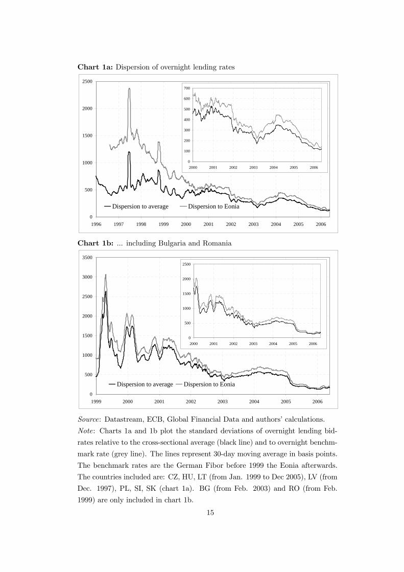
Chart 1a: Dispersion of overnight lending rates

0

500

1000

1500

2000

2500

1996 1997 1998 1999 2000 2001 2002 2003 2004 2005 2006

Dispersion to average Dispersion to Eonia

0

100

200

300

400

500

600

700

2000 2001 2002 2003 2004 2005 2006

Chart 1b: ... including Bulgaria and Romania

0

500

1000

1500

2000

2500

3000

3500

1999 2000 2001 2002 2003 2004 2005 2006

Dispersion to average Dispersion to Eonia

0

500

1000

1500

2000

2500

2000 2001 2002 2003 2004 2005 2006

Source: Datastream, ECB, Global Financial Data and authors’ calculations.

Note: Charts 1a and 1b plot the standard deviations of overnight lending bid-

rates relative to the cross-sectional average (black line) and to overnight benchm-

mark rate (grey line). The lines represent 30-day moving average in basis points.

The benchmark rates are the German Fibor before 1999 the Eonia afterwards.

The countries included are: CZ, HU, LT (from Jan. 1999 to Dec 2005), LV (from

Dec. 1997), PL, SI, SK (chart 1a). BG (from Feb. 2003) and RO (from Feb.

1999) are only included in chart 1b.

15

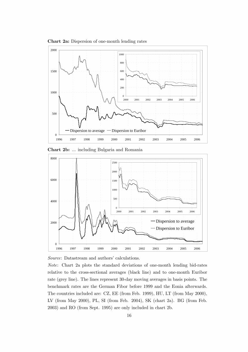
Chart 2a: Dispersion of one-month lending rates

0

500

1000

1500

2000

1996 1997 1998 1999 2000 2001 2002 2003 2004 2005 2006

Dispersion to average Dispersion to Euribor

0

200

400

600

800

1000

2000 2001 2002 2003 2004 2005 2006

Chart 2b: ... including Bulgaria and Romania

0

2000

4000

6000

8000

1996 1997 1998 1999 2000 2001 2002 2003 2004 2005 2006

Dispersion to averageDispersion to Euribor

0

500

1000

1500

2000

2500

2000 2001 2002 2003 2004 2005 2006

Source: Datastream and authors’ calculations.

Note: Chart 2a plots the standard deviations of one-month lending bid-rates

relative to the cross-sectional averages (black line) and to one-month Euribor

rate (grey line). The lines represent 30-day moving averages in basis points. The

benchmark rates are the German Fibor before 1999 and the Eonia afterwards.

The countries included are: CZ, EE (from Feb. 1999), HU, LT (from May 2000),

LV (from May 2000), PL, SI (from Feb. 2004), SK (chart 2a). BG (from Feb.

2003) and RO (from Sept. 1995) are only included in chart 2b.

16

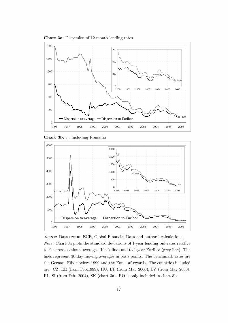
Chart 3a: Dispersion of 12-month lending rates

0

300

600

900

1200

1500

1800

1996 1997 1998 1999 2000 2001 2002 2003 2004 2005 2006

Dispersion to average Dispersion to Euribor

0

300

600

900

2000 2001 2002 2003 2004 2005 2006

Chart 3b: ... including Romania

0

1000

2000

3000

4000

5000

6000

1996 1997 1998 1999 2000 2001 2002 2003 2004 2005 2006

Dispersion to average Dispersion to Euribor

0

500

1000

1500

2000

2500

2000 2001 2002 2003 2004 2005 2006

Source: Datastream, ECB, Global Financial Data and authors’ calculations.

Note: Chart 3a plots the standard deviations of 1-year lending bid-rates relative

to the cross-sectional averages (black line) and to 1-year Euribor (grey line). The

lines represent 30-day moving averages in basis points. The benchmark rates are

the German Fibor before 1999 and the Eonia aftewards. The countries included

are: CZ, EE (from Feb.1999), HU, LT (from May 2000), LV (from May 2000),

PL, SI (from Feb. 2004), SK (chart 3a). RO is only included in chart 3b.

17

Charts 2a and 3a show a pattern similar to that of the overnight rate indicator.

The trend is decreasing, suggesting that integration is taking place. As for charts 2b

and 3b, we notice that the inclusion of Romania generates a substantial increase in

the dispersion of the first part of the sample (with dispersion spikes well above 6000

basis points), while convergence seems to take place over the last couple of years.12

Chart 4 reports the development of the dispersion in the one year swap rates.

The pattern of the indicator, and in particular the increase in dispersion around the

year 2004, reflects an increase in the Hungarian and to a less extent in the Polish

rates. Increases in these rates are in line with the other money market indicators

for Hungary and Poland. After the ratification of the Nice Treaty at the end of

2002, which primarily reformed the institutional structure of the European Union

to withstand the planned eastern enlargement, in Hungary there were fundamental

concerns about the fiscal discipline and continously elevated inflation expectations.

Figures at the end of the sample of charts 2-4 are roughly comparable with those

of the corresponding euro area markets in the run up to the EMU (see charts 3 and

7a of Baele et al, 2004).

12 In the first half of 1997 the Romanian leu depreciated sharply as a result of liberalisation of the

foreign exchange market and relatively higher inflation rates. Note that chart 3b does not include

Bulgaria due to lack of data.

18

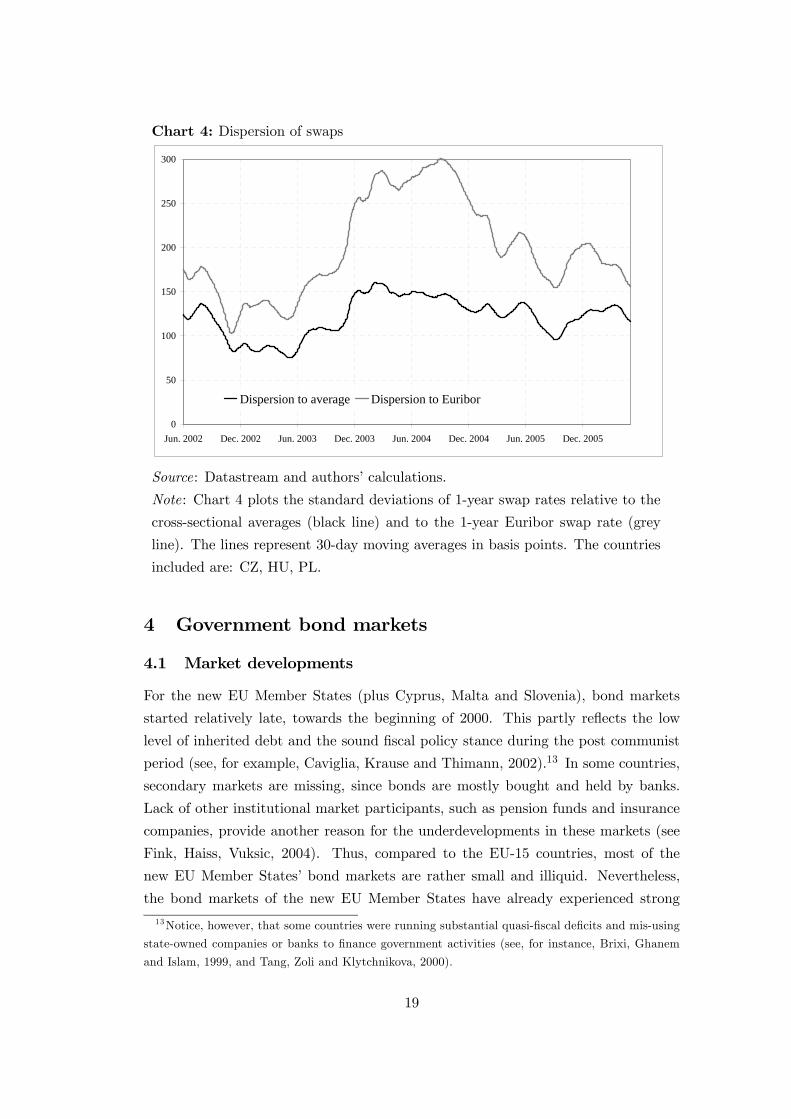
Chart 4: Dispersion of swaps

0

50

100

150

200

250

300

Jun. 2002 Dec. 2002 Jun. 2003 Dec. 2003 Jun. 2004 Dec. 2004 Jun. 2005 Dec. 2005

Dispersion to average Dispersion to Euribor

Source: Datastream and authors’ calculations.

Note: Chart 4 plots the standard deviations of 1-year swap rates relative to the

cross-sectional averages (black line) and to the 1-year Euribor swap rate (grey

line). The lines represent 30-day moving averages in basis points. The countries

included are: CZ, HU, PL.

4 Government bond markets

4.1 Market developments

For the new EU Member States (plus Cyprus, Malta and Slovenia), bond markets

started relatively late, towards the beginning of 2000. This partly reflects the low

level of inherited debt and the sound fiscal policy stance during the post communist

period (see, for example, Caviglia, Krause and Thimann, 2002).13 In some countries,

secondary markets are missing, since bonds are mostly bought and held by banks.

Lack of other institutional market participants, such as pension funds and insurance

companies, provide another reason for the underdevelopments in these markets (see

Fink, Haiss, Vuksic, 2004). Thus, compared to the EU-15 countries, most of the

new EU Member States’ bond markets are rather small and illiquid. Nevertheless,

the bond markets of the new EU Member States have already experienced strong

13Notice, however, that some countries were running substantial quasi-fiscal deficits and mis-using

state-owned companies or banks to finance government activities (see, for instance, Brixi, Ghanem

and Islam, 1999, and Tang, Zoli and Klytchnikova, 2000).

19

development. From 2000 to 2004 the ratio of outstanding government debt relative

to GDP more than doubled (see table 21 in Allen, Bartiloro, and Kowalewski, 2005).

While the proportion of domestic government debt securities relative to GDP in 2004

was 80% for the EU-15, the weighted average of the 10 new EU Member States (plus

Cyprus, Malta and Slovenia and excluding Bulgaria and Romania) was less than

55%. Yet, new EU Member States’ bond markets are still characterised by significant

structural differences.14

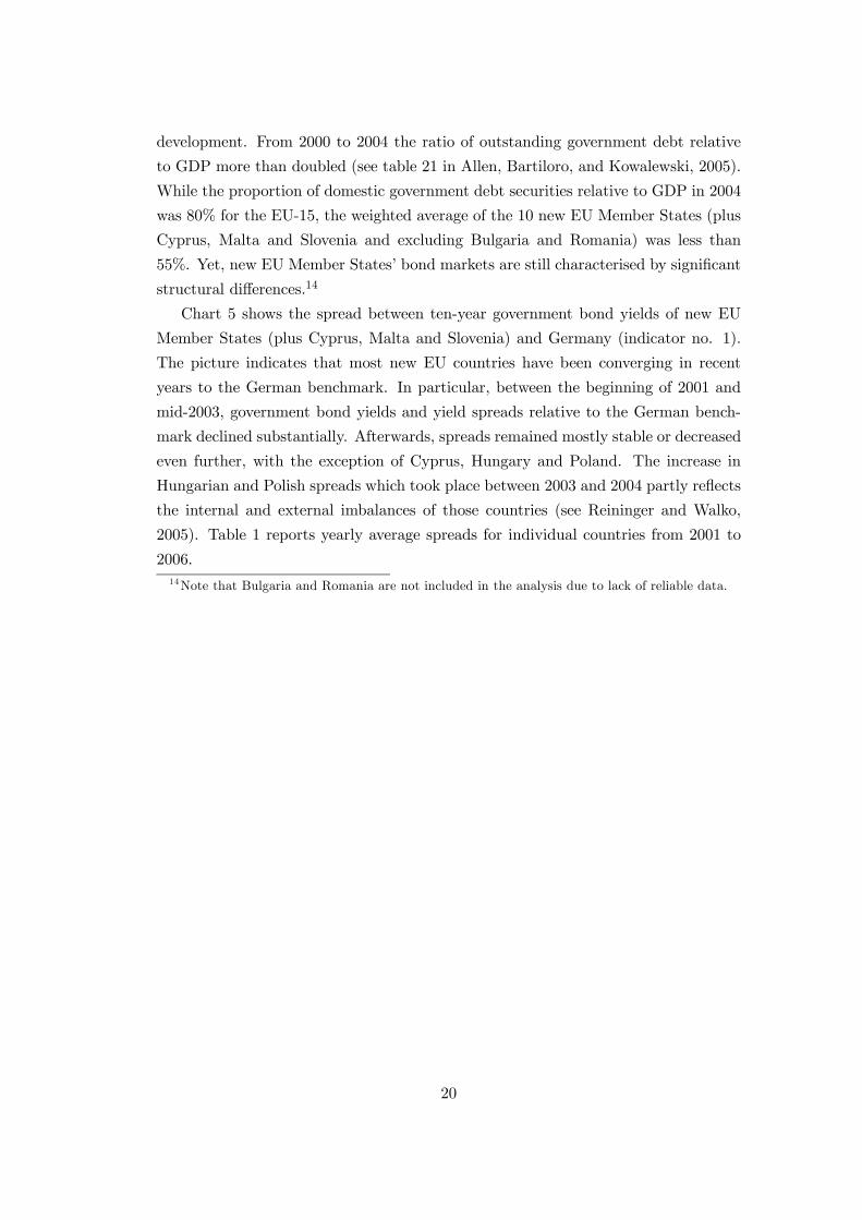
Chart 5 shows the spread between ten-year government bond yields of new EU

Member States (plus Cyprus, Malta and Slovenia) and Germany (indicator no. 1).

The picture indicates that most new EU countries have been converging in recent

years to the German benchmark. In particular, between the beginning of 2001 and

mid-2003, government bond yields and yield spreads relative to the German bench-

mark declined substantially. Afterwards, spreads remained mostly stable or decreased

even further, with the exception of Cyprus, Hungary and Poland. The increase in

Hungarian and Polish spreads which took place between 2003 and 2004 partly reflects

the internal and external imbalances of those countries (see Reininger and Walko,

2005). Table 1 reports yearly average spreads for individual countries from 2001 to

2006.14Note that Bulgaria and Romania are not included in the analysis due to lack of reliable data.

20

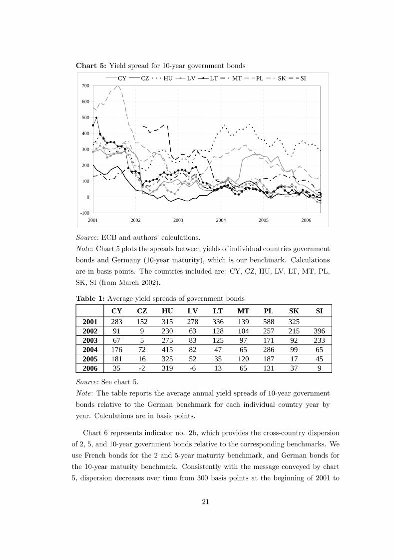
Chart 5: Yield spread for 10-year government bonds

-100

0

100

200

300

400

500

600

700

2001 2002 2003 2004 2005 2006

CY CZ HU LV LT MT PL SK SI

Source: ECB and authors’ calculations.

Note: Chart 5 plots the spreads between yields of individual countries government

bonds and Germany (10-year maturity), which is our benchmark. Calculations

are in basis points. The countries included are: CY, CZ, HU, LV, LT, MT, PL,

SK, SI (from March 2002).

Table 1: Average yield spreads of government bonds

CY CZ HU LV LT MT PL SK SI2001 283 152 315 278 336 139 588 3252002 91 9 230 63 128 104 257 215 3962003 67 5 275 83 125 97 171 92 2332004 176 72 415 82 47 65 286 99 652005 181 16 325 52 35 120 187 17 452006 35 -2 319 -6 13 65 131 37 9

Source: See chart 5.

Note: The table reports the average annual yield spreads of 10-year government

bonds relative to the German benchmark for each individual country year by

year. Calculations are in basis points.

Chart 6 represents indicator no. 2b, which provides the cross-country dispersion

of 2, 5, and 10-year government bonds relative to the corresponding benchmarks. We

use French bonds for the 2 and 5-year maturity benchmark, and German bonds for

the 10-year maturity benchmark. Consistently with the message conveyed by chart

5, dispersion decreases over time from 300 basis points at the beginning of 2001 to

21

about 50 basis points in 2006. Analogous measures for euro area countries show that

spreads have followed similar developments, hovering around 200 basis points around

1996, before plunging towards zero in the run up to the EMU (see charts 9 and 10 of

Baele et al. 2004).

Chart 6: Average yield spread for government bonds with different maturities

0

100

200

300

400

2001 2002 2003 2004 2005 2006

10 Year 5 Year 2 Year

Source: ECB; benchmarks: German 10-year and French 5-, and 2-years govern-

ment bonds; available data: 10 Year average: CY, CZ, HU, LV, LT, MT, PL, SK,

SI (from 3/02); 5 Year average: CY (with gaps), CZ, HU, LV, LT (with gaps),

MT, PL, SK (with gaps), SI (with gaps); 2 Year average: CY (with gaps), CZ

(till 9/01), HU (till 12/01), LV (till 11/01), LT (with gaps), MT, PL, SK (with

gaps), SI (with gaps).

Note: Chart 6 plots the average spread in basis points between yields in the new

EU member states and the French and German benchmarks’ government bond

markets.

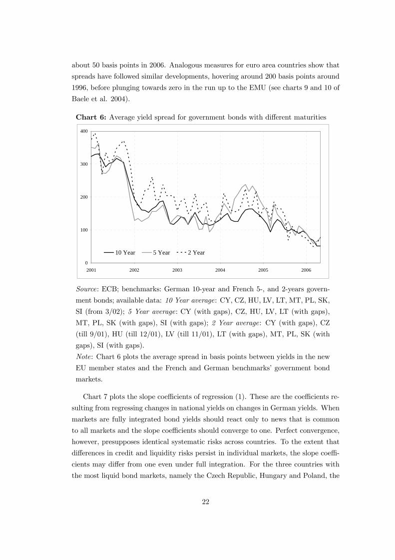
Chart 7 plots the slope coefficients of regression (1). These are the coefficients re-

sulting from regressing changes in national yields on changes in German yields. When

markets are fully integrated bond yields should react only to news that is common

to all markets and the slope coefficients should converge to one. Perfect convergence,

however, presupposes identical systematic risks across countries. To the extent that

differences in credit and liquidity risks persist in individual markets, the slope coeffi-

cients may differ from one even under full integration. For the three countries with

the most liquid bond markets, namely the Czech Republic, Hungary and Poland, the

22

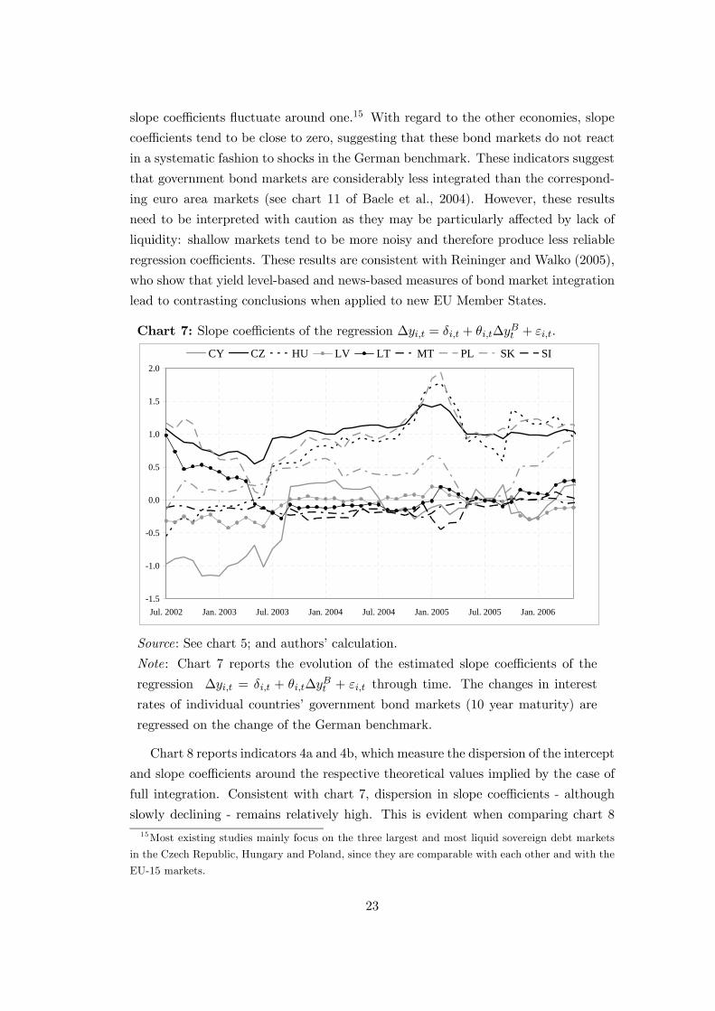
slope coefficients fluctuate around one.15 With regard to the other economies, slope

coefficients tend to be close to zero, suggesting that these bond markets do not react

in a systematic fashion to shocks in the German benchmark. These indicators suggest

that government bond markets are considerably less integrated than the correspond-

ing euro area markets (see chart 11 of Baele et al., 2004). However, these results

need to be interpreted with caution as they may be particularly affected by lack of

liquidity: shallow markets tend to be more noisy and therefore produce less reliable

regression coefficients. These results are consistent with Reininger and Walko (2005),

who show that yield level-based and news-based measures of bond market integration

lead to contrasting conclusions when applied to new EU Member States.

Chart 7: Slope coefficients of the regression ∆yi,t = δi,t + θi,t∆yBt + εi,t.

-1.5

-1.0

-0.5

0.0

0.5

1.0

1.5

2.0

Jul. 2002 Jan. 2003 Jul. 2003 Jan. 2004 Jul. 2004 Jan. 2005 Jul. 2005 Jan. 2006

CY CZ HU LV LT MT PL SK SI

Source: See chart 5; and authors’ calculation.

Note: Chart 7 reports the evolution of the estimated slope coefficients of the

regression ∆yi,t = δi,t + θi,t∆yBt + εi,t through time. The changes in interest

rates of individual countries’ government bond markets (10 year maturity) are

regressed on the change of the German benchmark.

Chart 8 reports indicators 4a and 4b, which measure the dispersion of the intercept

and slope coefficients around the respective theoretical values implied by the case of

full integration. Consistent with chart 7, dispersion in slope coefficients - although

slowly declining - remains relatively high. This is evident when comparing chart 815Most existing studies mainly focus on the three largest and most liquid sovereign debt markets

in the Czech Republic, Hungary and Poland, since they are comparable with each other and with the

EU-15 markets.

23

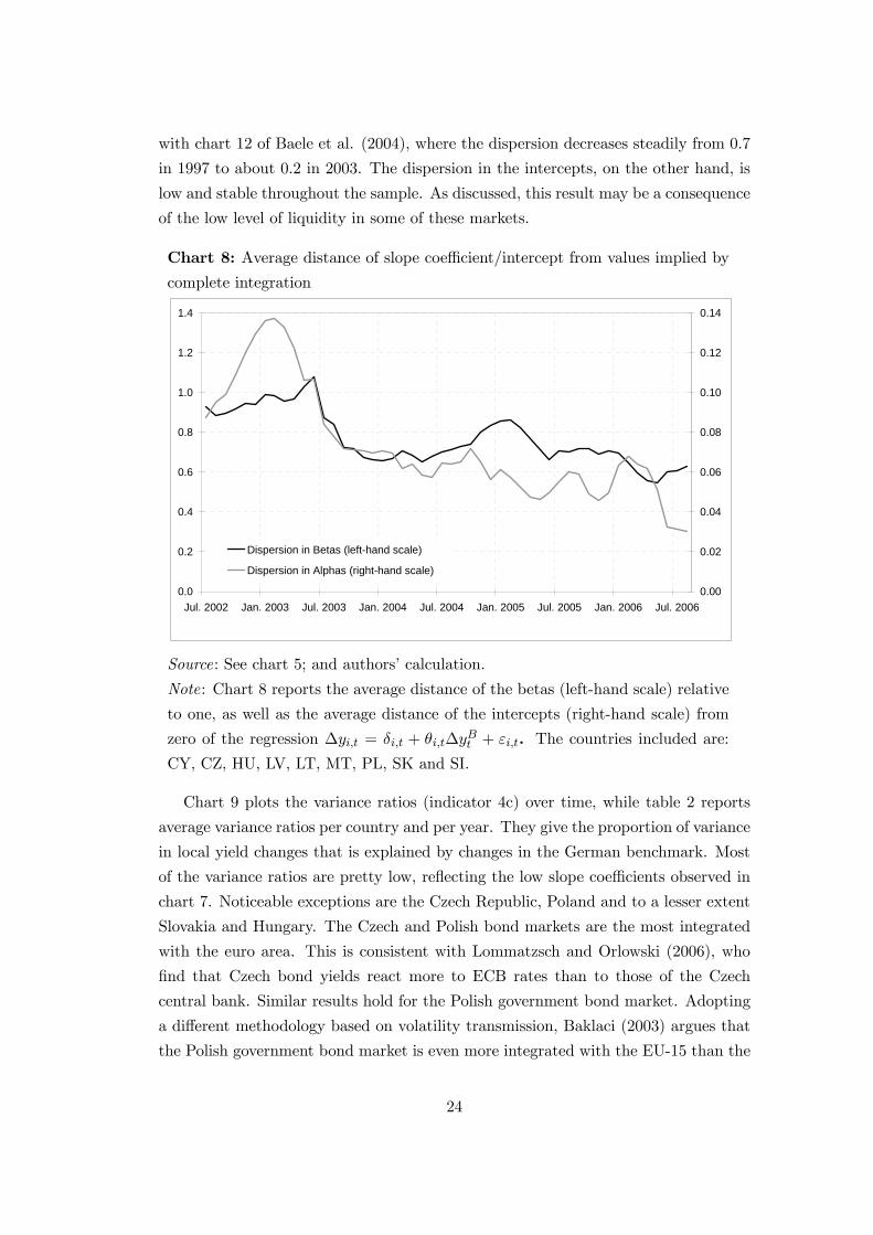
with chart 12 of Baele et al. (2004), where the dispersion decreases steadily from 0.7

in 1997 to about 0.2 in 2003. The dispersion in the intercepts, on the other hand, is

low and stable throughout the sample. As discussed, this result may be a consequence

of the low level of liquidity in some of these markets.

Chart 8: Average distance of slope coefficient/intercept from values implied by

complete integration

0.0

0.2

0.4

0.6

0.8

1.0

1.2

1.4

Jul. 2002 Jan. 2003 Jul. 2003 Jan. 2004 Jul. 2004 Jan. 2005 Jul. 2005 Jan. 2006 Jul. 20060.00

0.02

0.04

0.06

0.08

0.10

0.12

0.14

Dispersion in Betas (left-hand scale)

Dispersion in Alphas (right-hand scale)

Source: See chart 5; and authors’ calculation.

Note: Chart 8 reports the average distance of the betas (left-hand scale) relative

to one, as well as the average distance of the intercepts (right-hand scale) from

zero of the regression ∆yi,t = δi,t + θi,t∆yBt + εi,t. The countries included are:

CY, CZ, HU, LV, LT, MT, PL, SK and SI.

Chart 9 plots the variance ratios (indicator 4c) over time, while table 2 reports

average variance ratios per country and per year. They give the proportion of variance

in local yield changes that is explained by changes in the German benchmark. Most

of the variance ratios are pretty low, reflecting the low slope coefficients observed in

chart 7. Noticeable exceptions are the Czech Republic, Poland and to a lesser extent

Slovakia and Hungary. The Czech and Polish bond markets are the most integrated

with the euro area. This is consistent with Lommatzsch and Orlowski (2006), who

find that Czech bond yields react more to ECB rates than to those of the Czech

central bank. Similar results hold for the Polish government bond market. Adopting

a different methodology based on volatility transmission, Baklaci (2003) argues that

the Polish government bond market is even more integrated with the EU-15 than the

24

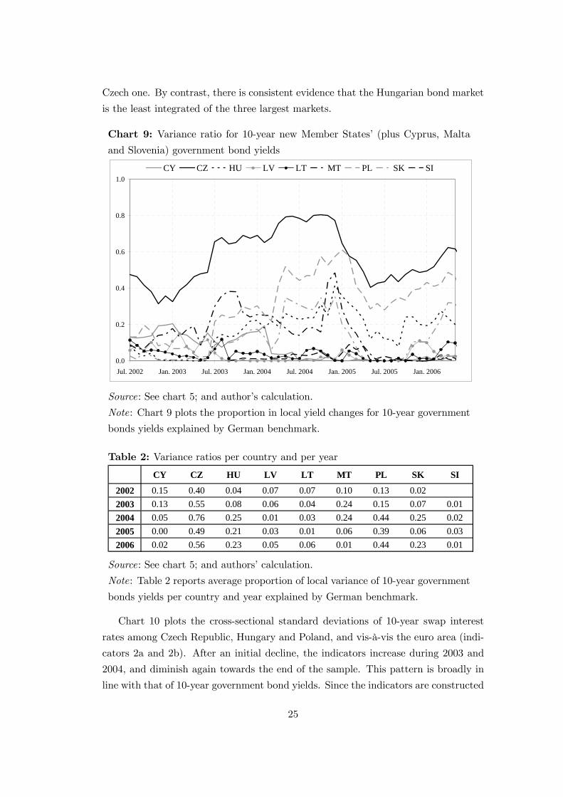
Czech one. By contrast, there is consistent evidence that the Hungarian bond market

is the least integrated of the three largest markets.

Chart 9: Variance ratio for 10-year new Member States’ (plus Cyprus, Malta

and Slovenia) government bond yields

0.0

0.2

0.4

0.6

0.8

1.0

Jul. 2002 Jan. 2003 Jul. 2003 Jan. 2004 Jul. 2004 Jan. 2005 Jul. 2005 Jan. 2006

CY CZ HU LV LT MT PL SK SI

Source: See chart 5; and author’s calculation.

Note: Chart 9 plots the proportion in local yield changes for 10-year government

bonds yields explained by German benchmark.

Table 2: Variance ratios per country and per year

CY CZ HU LV LT MT PL SK SI

2002 0.15 0.40 0.04 0.07 0.07 0.10 0.13 0.022003 0.13 0.55 0.08 0.06 0.04 0.24 0.15 0.07 0.012004 0.05 0.76 0.25 0.01 0.03 0.24 0.44 0.25 0.022005 0.00 0.49 0.21 0.03 0.01 0.06 0.39 0.06 0.032006 0.02 0.56 0.23 0.05 0.06 0.01 0.44 0.23 0.01

Source: See chart 5; and authors’ calculation.

Note: Table 2 reports average proportion of local variance of 10-year government

bonds yields per country and year explained by German benchmark.

Chart 10 plots the cross-sectional standard deviations of 10-year swap interest

rates among Czech Republic, Hungary and Poland, and vis-à-vis the euro area (indi-

cators 2a and 2b). After an initial decline, the indicators increase during 2003 and

2004, and diminish again towards the end of the sample. This pattern is broadly in

line with that of 10-year government bond yields. Since the indicators are constructed

25

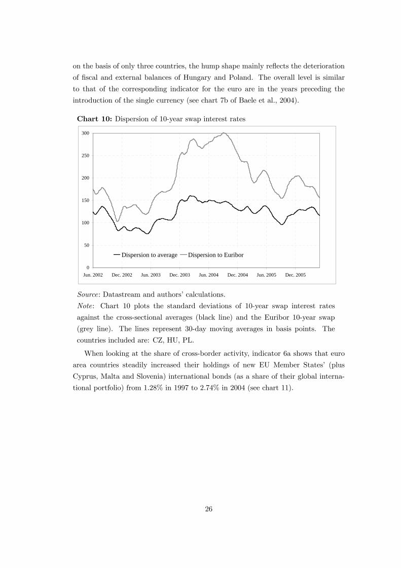
on the basis of only three countries, the hump shape mainly reflects the deterioration

of fiscal and external balances of Hungary and Poland. The overall level is similar

to that of the corresponding indicator for the euro are in the years preceding the

introduction of the single currency (see chart 7b of Baele et al., 2004).

Chart 10: Dispersion of 10-year swap interest rates

0

50

100

150

200

250

300

Jun. 2002 Dec. 2002 Jun. 2003 Dec. 2003 Jun. 2004 Dec. 2004 Jun. 2005 Dec. 2005

Dispersion to average Dispersion to Euribor

Source: Datastream and authors’ calculations.

Note: Chart 10 plots the standard deviations of 10-year swap interest rates

against the cross-sectional averages (black line) and the Euribor 10-year swap

(grey line). The lines represent 30-day moving averages in basis points. The

countries included are: CZ, HU, PL.

When looking at the share of cross-border activity, indicator 6a shows that euro

area countries steadily increased their holdings of new EU Member States’ (plus

Cyprus, Malta and Slovenia) international bonds (as a share of their global interna-

tional portfolio) from 1.28% in 1997 to 2.74% in 2004 (see chart 11).

26

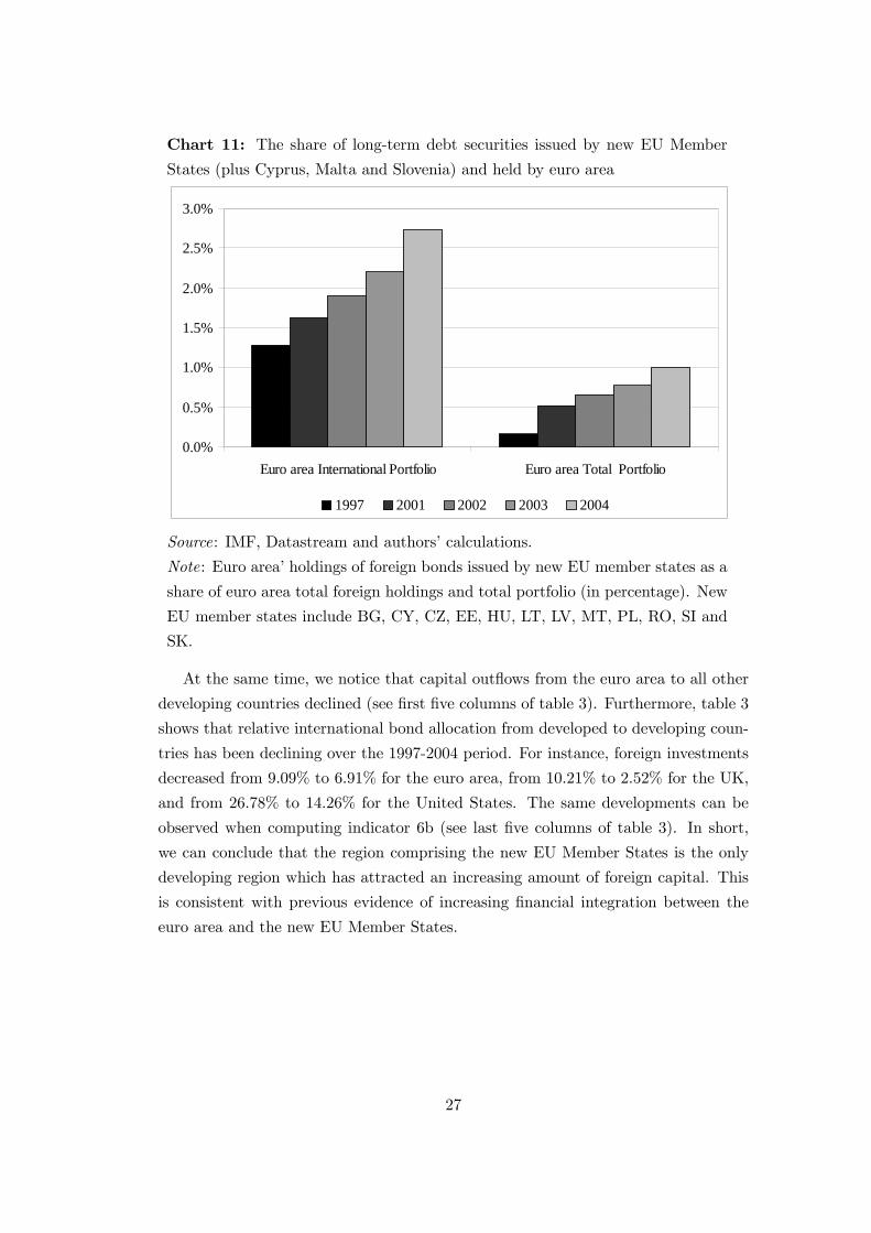
Chart 11: The share of long-term debt securities issued by new EU Member

States (plus Cyprus, Malta and Slovenia) and held by euro area

0.0%

0.5%

1.0%

1.5%

2.0%

2.5%

3.0%

Euro area International Portfolio Euro area Total Portfolio

1997 2001 2002 2003 2004

Source: IMF, Datastream and authors’ calculations.

Note: Euro area’ holdings of foreign bonds issued by new EU member states as a

share of euro area total foreign holdings and total portfolio (in percentage). New

EU member states include BG, CY, CZ, EE, HU, LT, LV, MT, PL, RO, SI and

SK.

At the same time, we notice that capital outflows from the euro area to all other

developing countries declined (see first five columns of table 3). Furthermore, table 3

shows that relative international bond allocation from developed to developing coun-

tries has been declining over the 1997-2004 period. For instance, foreign investments

decreased from 9.09% to 6.91% for the euro area, from 10.21% to 2.52% for the UK,

and from 26.78% to 14.26% for the United States. The same developments can be

observed when computing indicator 6b (see last five columns of table 3). In short,

we can conclude that the region comprising the new EU Member States is the only

developing region which has attracted an increasing amount of foreign capital. This

is consistent with previous evidence of increasing financial integration between the

euro area and the new EU Member States.

27

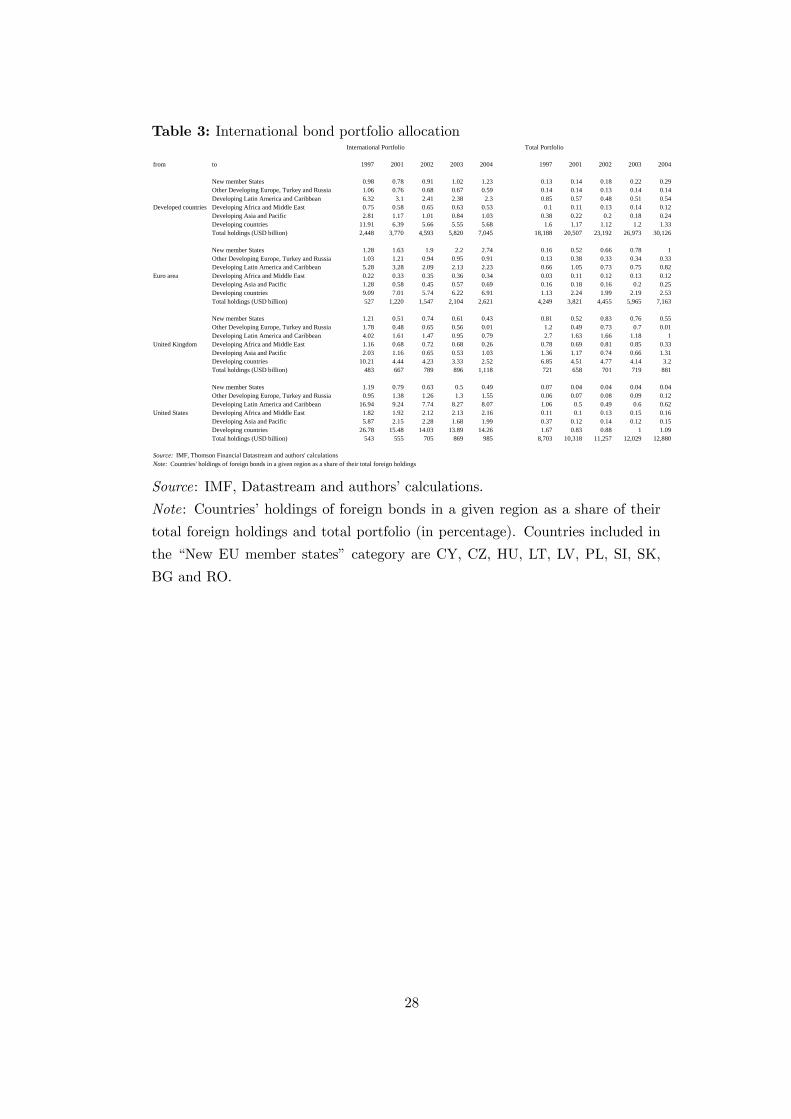
Table 3: International bond portfolio allocationInternational Portfolio Total Portfolio

from to 1997 2001 2002 2003 2004 1997 2001 2002 2003 2004

New member States 0.98 0.78 0.91 1.02 1.23 0.13 0.14 0.18 0.22 0.29Other Developing Europe, Turkey and Russia 1.06 0.76 0.68 0.67 0.59 0.14 0.14 0.13 0.14 0.14Developing Latin America and Caribbean 6.32 3.1 2.41 2.38 2.3 0.85 0.57 0.48 0.51 0.54

Developed countries Developing Africa and Middle East 0.75 0.58 0.65 0.63 0.53 0.1 0.11 0.13 0.14 0.12Developing Asia and Pacific 2.81 1.17 1.01 0.84 1.03 0.38 0.22 0.2 0.18 0.24Developing countries 11.91 6.39 5.66 5.55 5.68 1.6 1.17 1.12 1.2 1.33Total holdings (USD billion) 2,448 3,770 4,593 5,820 7,045 18,188 20,507 23,192 26,973 30,126

New member States 1.28 1.63 1.9 2.2 2.74 0.16 0.52 0.66 0.78 1Other Developing Europe, Turkey and Russia 1.03 1.21 0.94 0.95 0.91 0.13 0.38 0.33 0.34 0.33Developing Latin America and Caribbean 5.28 3.28 2.09 2.13 2.23 0.66 1.05 0.73 0.75 0.82

Euro area Developing Africa and Middle East 0.22 0.33 0.35 0.36 0.34 0.03 0.11 0.12 0.13 0.12Developing Asia and Pacific 1.28 0.58 0.45 0.57 0.69 0.16 0.18 0.16 0.2 0.25Developing countries 9.09 7.01 5.74 6.22 6.91 1.13 2.24 1.99 2.19 2.53Total holdings (USD billion) 527 1,220 1,547 2,104 2,621 4,249 3,821 4,455 5,965 7,163

New member States 1.21 0.51 0.74 0.61 0.43 0.81 0.52 0.83 0.76 0.55Other Developing Europe, Turkey and Russia 1.78 0.48 0.65 0.56 0.01 1.2 0.49 0.73 0.7 0.01Developing Latin America and Caribbean 4.02 1.61 1.47 0.95 0.79 2.7 1.63 1.66 1.18 1

United Kingdom Developing Africa and Middle East 1.16 0.68 0.72 0.68 0.26 0.78 0.69 0.81 0.85 0.33Developing Asia and Pacific 2.03 1.16 0.65 0.53 1.03 1.36 1.17 0.74 0.66 1.31Developing countries 10.21 4.44 4.23 3.33 2.52 6.85 4.51 4.77 4.14 3.2Total holdings (USD billion) 483 667 789 896 1,118 721 658 701 719 881

New member States 1.19 0.79 0.63 0.5 0.49 0.07 0.04 0.04 0.04 0.04Other Developing Europe, Turkey and Russia 0.95 1.38 1.26 1.3 1.55 0.06 0.07 0.08 0.09 0.12Developing Latin America and Caribbean 16.94 9.24 7.74 8.27 8.07 1.06 0.5 0.49 0.6 0.62

United States Developing Africa and Middle East 1.82 1.92 2.12 2.13 2.16 0.11 0.1 0.13 0.15 0.16Developing Asia and Pacific 5.87 2.15 2.28 1.68 1.99 0.37 0.12 0.14 0.12 0.15Developing countries 26.78 15.48 14.03 13.89 14.26 1.67 0.83 0.88 1 1.09Total holdings (USD billion) 543 555 705 869 985 8,703 10,318 11,257 12,029 12,880

Source: IMF, Thomson Financial Datastream and authors' calculationsNote: Countries' holdings of foreign bonds in a given region as a share of their total foreign holdings

Source: IMF, Datastream and authors’ calculations.

Note: Countries’ holdings of foreign bonds in a given region as a share of their

total foreign holdings and total portfolio (in percentage). Countries included in

the “New EU member states” category are CY, CZ, HU, LT, LV, PL, SI, SK,

BG and RO.

28

5 Banking markets

With regard to the banking markets of new EU Member States (plus Cyprus, Malta

and Slovenia), data on interest rates on mortgage loans, consumer loans, as well as

short, medium and long-term loans to enterprises are analysed.

Over the past decade, foreign banks have significantly expanded their presence in

the new EU Member States (ECB 2005c). In 2003, on average more than 70% of

bank assets were foreign-owned ranging from more than 95% in the Czech Republic,

Estonia, Lithuania and Slovakia to 36% in Slovenia and 12% in Cyprus. The most

common foreign presence is in the form of subsidiaries, while the number of branches

remains very limited. Nordic banks have become active in the Baltic States, and

Austrian and Italian banks are operating in neighbouring central European countries

(the Czech Republic, Hungary and Slovakia). The strong foreign (mainly European)

presence in the new EU Member States is widely believed to be beneficial for the

banking systems due to the transfer of technology and human capital, which increases

the operational capacity of local banks and accelerates convergence with western

standards (ECB 2006b, Moody’s 2004).

Charts 12a-b and 13a-c plot the loans’ cross-sectional standard deviations since

the second half of the 1990’s. The data for Bulgaria are reported separately, since

they all exhibit large spikes around 1996. In that year, the country suffered from a

severe crisis of confidence in the banking system, which led to a currency collapse.16

Since the spikes affect the overall scale of the charts, for comparability purposes, the

indicators for the last part of the sample are reported in separate charts. Standard

deviations broadly decrease for all the loan rates from 1995 onwards (the same holds

true for the statistics that include Bulgaria). Decrease in dispersion indicates that

rates across new EU Member States (plus Cyprus, Malta and Slovenia) have become

progressively more homogeneous, suggesting that integration across these markets is

increasing. The hump shape observed around 2004 is similar to that observed for

swap rates in charts 4 and 10. This is due to an increase in Hungarian rates, which

in turn reflects the deterioration of Hungary’s fiscal and external balance.17

16Data for Romania are not available.17There is no hump in the medium and long-term loans indicators since they do not include

Hungarian data.

29

Chart 12a: Dispersion of loans to enterprises

0

1000

2000

3000

4000

1996 1997 1998 1999 2000 2001 2002 2003 2004 2005 2006

Short-term loans

Medium- and long-term loans

0

200

400

600

800

1000

1200

2000 2001 2002 2003 2004 2005 2006

Chart 12b: ... including Bulgaria

0

2000000

4000000

6000000

8000000

10000000

12000000

1996 1997 1998 1999 2000 2001 2002 2003 2004 2005 2006

Short-term loans Medium- and long-term loans

0

200

400

600

800

1000

1200

2000 2001 2002 2003 2004 2005 2006

Source: Global Financial Data and authors’ calculation.

Note: Charts 12a and 12b plot average cross-sectional standard deviations (in

basis points) of interest rates on short and long-term loans to enterprises relative

to the cross-sectional averages. Data for short-term loans are available for: CZ,

EE, HU, LT, LV (chart 12a). BG is only included in chart 12b. Data for medium

and long-term loans are available for CZ, EE, LT, LV, MT (from Jan. 2000), SI,

SK (chart 12a). BG is only included in chart 12b.30

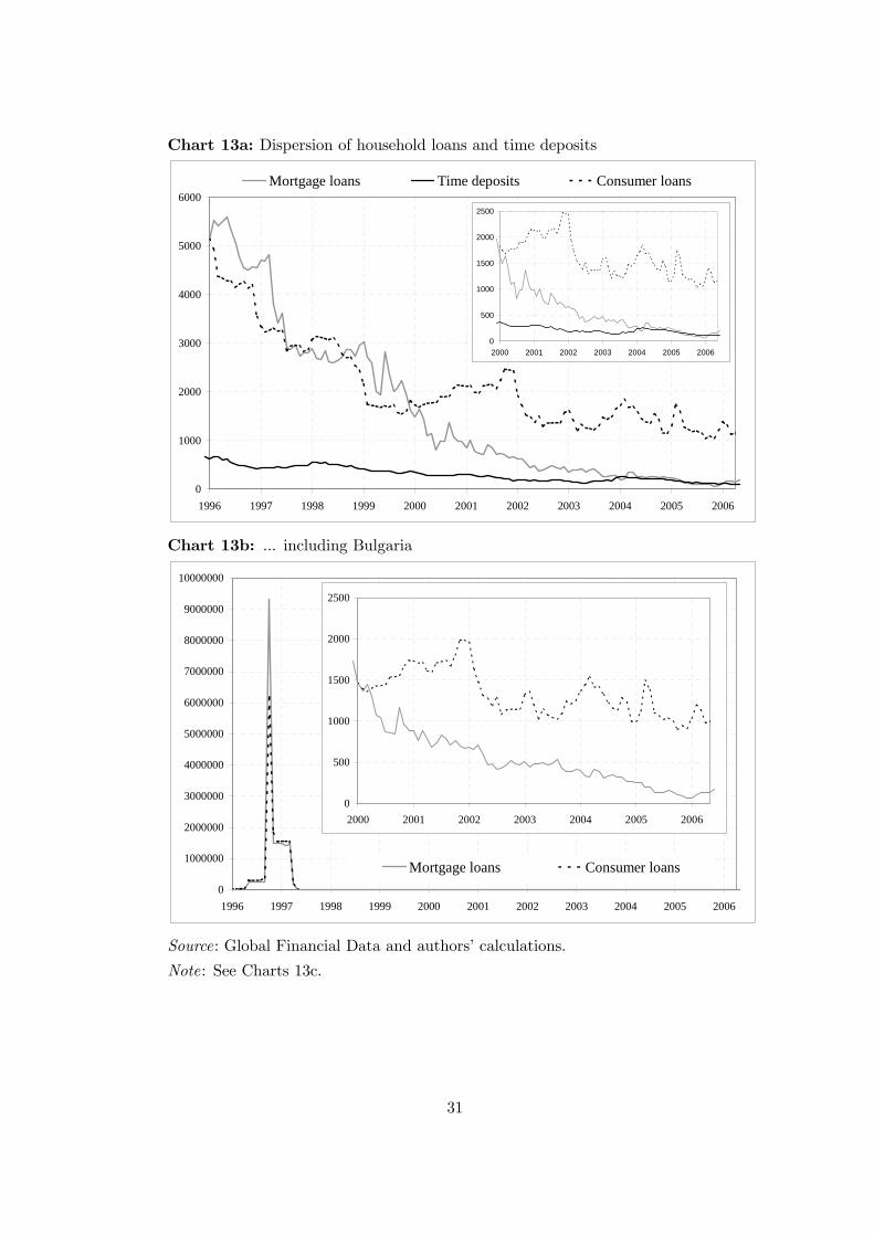
Chart 13a: Dispersion of household loans and time deposits

0

1000

2000

3000

4000

5000

6000

1996 1997 1998 1999 2000 2001 2002 2003 2004 2005 2006

Mortgage loans Time deposits Consumer loans

0

500

1000

1500

2000

2500

2000 2001 2002 2003 2004 2005 2006

Chart 13b: ... including Bulgaria

0

1000000

2000000

3000000

4000000

5000000

6000000

7000000

8000000

9000000

10000000

1996 1997 1998 1999 2000 2001 2002 2003 2004 2005 2006

Mortgage loans Consumer loans

0

500

1000

1500

2000

2500

2000 2001 2002 2003 2004 2005 2006

Source: Global Financial Data and authors’ calculations.

Note: See Charts 13c.

31

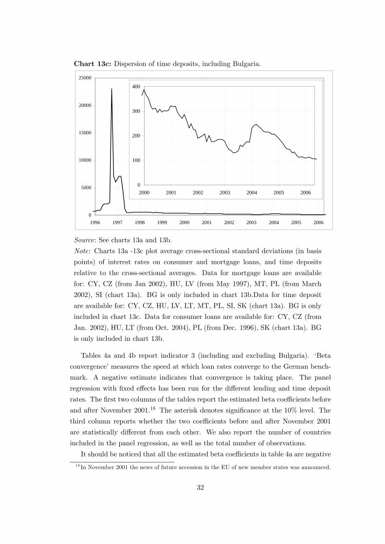
Chart 13c: Dispersion of time deposits, including Bulgaria.

0

5000

10000

15000

20000

25000

1996 1997 1998 1999 2000 2001 2002 2003 2004 2005 2006

0

100

200

300

400

2000 2001 2002 2003 2004 2005 2006

Source: See charts 13a and 13b.

Note: Charts 13a -13c plot average cross-sectional standard deviations (in basis

points) of interest rates on consumer and mortgage loans, and time deposits

relative to the cross-sectional averages. Data for mortgage loans are available

for: CY, CZ (from Jan 2002), HU, LV (from May 1997), MT, PL (from March

2002), SI (chart 13a). BG is only included in chart 13b.Data for time deposit

are available for: CY, CZ, HU, LV, LT, MT, PL, SI, SK (chart 13a). BG is only

included in chart 13c. Data for consumer loans are available for: CY, CZ (from

Jan. 2002), HU, LT (from Oct. 2004), PL (from Dec. 1996), SK (chart 13a). BG

is only included in chart 13b.

Tables 4a and 4b report indicator 3 (including and excluding Bulgaria). ‘Beta

convergence’ measures the speed at which loan rates converge to the German bench-

mark. A negative estimate indicates that convergence is taking place. The panel

regression with fixed effects has been run for the different lending and time deposit

rates. The first two columns of the tables report the estimated beta coefficients before

and after November 2001.18 The asterisk denotes significance at the 10% level. The

third column reports whether the two coefficients before and after November 2001

are statistically different from each other. We also report the number of countries

included in the panel regression, as well as the total number of observations.

It should be noticed that all the estimated beta coefficients in table 4a are negative

18 In November 2001 the news of future accession in the EU of new member states was announced.

32

and statistically different from zero (time deposit rates after November 2001 being

the only exception). Furthermore, for short-term loans to enterprises and mortgage

loans to households, the speed of convergence increases in a statistically significant

way after November 2001. When Bulgaria is included in the analysis (table 4b), all

the betas remain negative, but are not always significant after 2001. All in all, these

results suggest that the loan rate markets are becoming increasingly integrated.

33

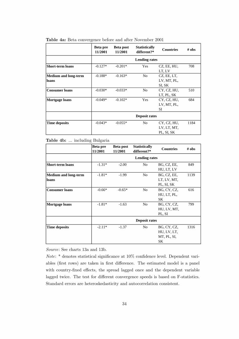
Table 4a: Beta convergence before and after November 2001

Beta pre 11/2001

Beta post 11/2001

Statistically different?* Countries # obs

Short-term loans -0.127* -0.201* Yes CZ, EE, HU, LT, LV

708

Medium and long-term loans

-0.188* -0.163* No CZ, EE, LT, LV, MT, PL, SI, SK

Consumer loans -0.030* -0.033* No CY, CZ, HU, LT, PL, SK

510

Mortgage loans -0.049* -0.102* Yes CY, CZ, HU, LV, MT, PL, SI

684

Time deposits -0.043* -0.055* No CY, CZ, HU, LV, LT, MT, PL, SI, SK

1184

Lending rates

Deposit rates

Table 4b: ... including BulgariaBeta pre 11/2001

Beta post 11/2001

Statistically different?* Countries # obs

Short-term loans -1.31* -2.00 No BG, CZ, EE, HU, LT, LV

849

Medium and long-term loans

-1.81* -1.99 No BG, CZ, EE, LT, LV, MT, PL, SI, SK

1139

Consumer loans -0.66* -0.65* No BG, CY, CZ, HU, LT, PL, SK

616

Mortgage loans -1.81* -1.63 No BG, CY, CZ, HU, LV, MT, PL, SI

799

Time deposits -2.11* -1.37 No BG, CY, CZ, HU, LV, LT, MT, PL, SI, SK

1316

Lending rates

Deposit rates

Source: See charts 13a and 13b.

Note: * denotes statistical significance at 10% confidence level. Dependent vari-

ables (first rows) are taken in first difference. The estimated model is a panel

with country-fixed effects, the spread lagged once and the dependent variable

lagged twice. The test for different convergence speeds is based on F-statistics.

Standard errors are heteroskedasticity and autocorrelation consistent.

34

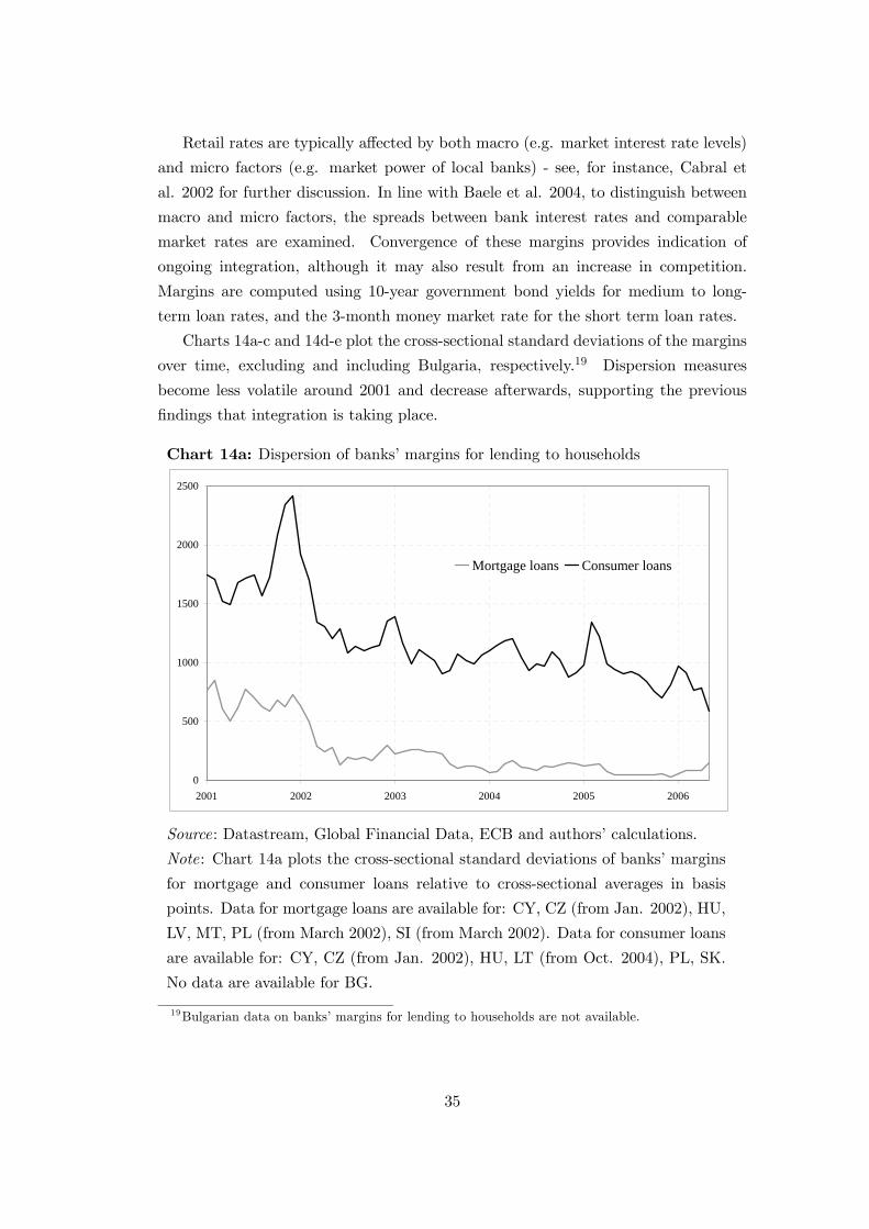
Retail rates are typically affected by both macro (e.g. market interest rate levels)

and micro factors (e.g. market power of local banks) - see, for instance, Cabral et

al. 2002 for further discussion. In line with Baele et al. 2004, to distinguish between

macro and micro factors, the spreads between bank interest rates and comparable

market rates are examined. Convergence of these margins provides indication of

ongoing integration, although it may also result from an increase in competition.

Margins are computed using 10-year government bond yields for medium to long-

term loan rates, and the 3-month money market rate for the short term loan rates.

Charts 14a-c and 14d-e plot the cross-sectional standard deviations of the margins

over time, excluding and including Bulgaria, respectively.19 Dispersion measures

become less volatile around 2001 and decrease afterwards, supporting the previous

findings that integration is taking place.

Chart 14a: Dispersion of banks’ margins for lending to households

0

500

1000

1500

2000

2500

2001 2002 2003 2004 2005 2006

Mortgage loans Consumer loans

Source: Datastream, Global Financial Data, ECB and authors’ calculations.

Note: Chart 14a plots the cross-sectional standard deviations of banks’ margins

for mortgage and consumer loans relative to cross-sectional averages in basis

points. Data for mortgage loans are available for: CY, CZ (from Jan. 2002), HU,

LV, MT, PL (from March 2002), SI (from March 2002). Data for consumer loans

are available for: CY, CZ (from Jan. 2002), HU, LT (from Oct. 2004), PL, SK.

No data are available for BG.

19Bulgarian data on banks’ margins for lending to households are not available.

35

Chart 14b: Dispersion of banks’ margins for time deposits

0

200

400

600

800

1996 1997 1998 1999 2000 2001 2002 2003 2004 2005 2006

0

100

200

300

2000 2001 2002 2003 2004 2005 2006

Chart 14c: ... including Bulgaria

0

100

200

300

400

1998 1999 2000 2001 2002 2003 2004 2005 2006

Source: Global Financial Data and authors’ calculations.

Note: Charts 14b and 14c plot the cross-sectional standard deviations of banks’

margins for time deposits relative to cross-sectional averages in basis points. The

countries included are: CY (from March 1999), CZ, HU, LV (from Jan. 1998),

LT (from Jan. 1999), MT (from Apr. 1996), PL, SI, SK (from Nov. 1998) (chart

14b). BG (from Jan. 1998) is only included in chart 14c.

36

Chart 14d: Dispersion of banks’ margins for lending to enterprises

0

1000

2000

3000

4000

5000

1996 1997 1998 1999 2000 2001 2002 2003 2004 2005 2006

Short-term loans Medium and long-term loans

0

100

200

300

400

500

600

700

2000 2001 2002 2003 2004 2005 2006

Chart 14e: Dispersion of banks’ margins for short-term lending to enterprises,

including Bulgaria

0

500

1000

1500

1998 1999 2000 2001 2002 2003 2004 2005 2006

Source: Global Financial Data and authors’ calculations.

Note: Charts 14d and 14e plot the cross-sectional standard deviations of banks’

margins for lending to enterprises relative to cross-sectional averages in basis

points. Data for short-term loans are available for: CZ, EE, HU, LV (from Jan.

1998), LT (from Jan. 1999) (chart 13d). BG (from Jan. 1998) is only included

in chart 13e. Data for medium- and long-term loans are available for: CZ, LV,

LT, MT, PL, SK, SI (from March 2002) (chart 13d).

37

Chart 15a: Proportion of variance of various interest rates explained by common

factors

0

0.1

0.2

0.3

0.4

0.5

0.6

short-term loans toenterprises

medium and long-term loans toenterprises

consumer loans mortgages time deposits

Pre-11/2001

Post-11/2001

Chart 15b: ... including Bulgaria

0

0.1

0.2

0.3

0.4

0.5

0.6

short-term loans toenterprises

medium and long-term loans toenterprises

consumer loans mortgages time deposits

Pre-11/2001

Post-11/2001

Source: See charts 14a-14e.

Note: Charts 15a and 15b report the average proportion of variance explained

by the German benchmarks.

38

Charts 15a-b show the proportion of loan and time deposit rate changes explained

by the relevant benchmark before and after November 2001 (indicator 4c). As usual

we distinguish between the sample excluding and including Bulgaria. The benchmarks

are the same interest rates employed in the construction of the margins of charts 14a-

e. To the extent that retail rates are comparable across countries, higher degrees of

integration imply a greater impact of common factors and higher variance ratios.

We observe that for short, medium and long-term loans to enterprises, as well as

for time deposits, the proportion of variance explained by common factors increases

over time, reaching levels comparable to those documented for the euro area countries

(see chart 25 in Baele et al. 2004). In line with the findings in the euro area, levels of

integration in consumer loans and mortgage markets appear to be consistently lower

than for the other markets. This result may reflect a lack of standardisation of these

products, as well as legal and consumer protection barriers in the different national

markets. When Bulgaria is included in the analysis, the proportions of variance ex-

plained by common factors decreases substantially, suggesting that Bulgarian markets

are characterised by a larger degree of heterogeneity.

A review of quantity-based indicators (indicator 6c) shows that the region com-

prising the new EU Member States (plus Cyprus, Malta and Slovenia) is the only one

among developing countries that has been receiving a steadily increasing percentage

of bank loans (see Chart 16a). This development is entirely due to the expansion of

credit from euro area banks, as shown in charts 16b-d. According to chart 16b, the

percentage share of euro area outstanding loans vis-à-vis the new EU Member States

increased from 1.5% at the end of 1995 to 2.0% right before the Russian crisis at the

end of 1998, and up to 3.6% at the end of 2005. On the contrary, the analog indicator

has been declining for the UK (see chart 16c) and close to zero for the United States

(see chart 16d). Furthermore, the share allocated in other developing regions either

declines or does not show any clear trend.

The available evidence clearly indicates that the integration of banking activi-

ties among euro area countries and the new EU Member States is taking place and

deepening. This statement is even more significant if one considers the cross-border

investment at country level. The euro area has been increasing the share of its interna-

tional claims vis-à-vis each individual new EU Member State (plus Cyprus, Malta and

Slovenia), with the Czech Republic, Hungary and Poland being the most important

recipient countries (see chart 16e).

39

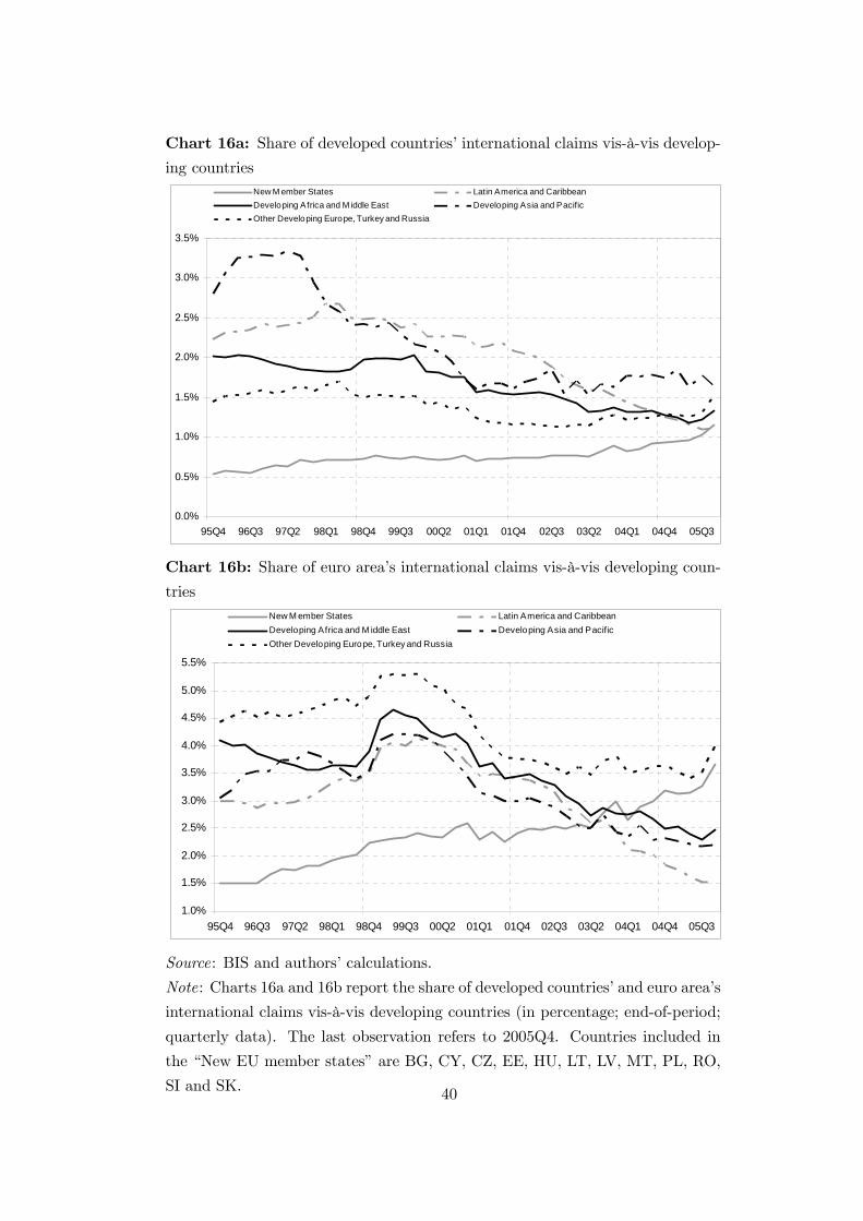
Chart 16a: Share of developed countries’ international claims vis-à-vis develop-

ing countries

0.0%

0.5%

1.0%

1.5%

2.0%

2.5%

3.0%

3.5%

95Q4 96Q3 97Q2 98Q1 98Q4 99Q3 00Q2 01Q1 01Q4 02Q3 03Q2 04Q1 04Q4 05Q3

New M ember States Latin America and CaribbeanDeveloping Africa and M iddle East Developing Asia and PacificOther Developing Europe, Turkey and Russia

Chart 16b: Share of euro area’s international claims vis-à-vis developing coun-

tries

1.0%

1.5%

2.0%

2.5%

3.0%

3.5%

4.0%

4.5%

5.0%

5.5%

95Q4 96Q3 97Q2 98Q1 98Q4 99Q3 00Q2 01Q1 01Q4 02Q3 03Q2 04Q1 04Q4 05Q3

New M ember States Latin America and CaribbeanDeveloping Africa and M iddle East Developing Asia and PacificOther Developing Europe, Turkey and Russia

Source: BIS and authors’ calculations.

Note: Charts 16a and 16b report the share of developed countries’ and euro area’s

international claims vis-à-vis developing countries (in percentage; end-of-period;

quarterly data). The last observation refers to 2005Q4. Countries included in

the “New EU member states” are BG, CY, CZ, EE, HU, LT, LV, MT, PL, RO,

SI and SK. 40

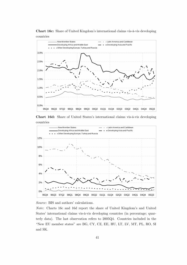
Chart 16c: Share of United Kingdom’s international claims vis-à-vis developing

countries

0.0%

0.5%

1.0%

1.5%

2.0%

2.5%

3.0%

95Q4 96Q3 97Q2 98Q1 98Q4 99Q3 00Q2 01Q1 01Q4 02Q3 03Q2 04Q1 04Q4 05Q3

New M ember States Latin America and CaribbeanDeveloping Africa and M iddle East Developing Asia and PacificOther Developing Europe, Turkey and Russia

Chart 16d: Share of United States’s international claims vis-à-vis developing

countries

0%

2%

4%

6%

8%

10%

12%

95Q4 96Q3 97Q2 98Q1 98Q4 99Q3 00Q2 01Q1 01Q4 02Q3 03Q2 04Q1 04Q4 05Q3

New M ember States Latin America and CaribbeanDeveloping Africa and M iddle East Developing Asia and PacificOther Developing Europe, Turkey and Russia

Source: BIS and authors’ calculations.

Note: Charts 16c and 16d report the share of United Kingdom’s and United

States’ international claims vis-à-vis developing countries (in percentage; quar-

terly data). The last observation refers to 2005Q4. Countries included in the

“New EU member states” are BG, CY, CZ, EE, HU, LT, LV, MT, PL, RO, SI

and SK.

41

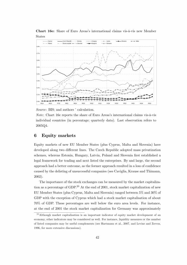
Chart 16e: Share of Euro Areas’s international claims vis-à-vis new Member

States

0.0%

0.1%

0.2%

0.3%

0.4%

0.5%

0.6%

0.7%

0.8%

95Q4 96Q3 97Q2 98Q1 98Q4 99Q3 00Q2 01Q1 01Q4 02Q3 03Q2 04Q1 04Q4 05Q3

Cyprus Czech Republic Estonia Hungary Latvia Lithuania Malta

Poland Slovak republic Slovenia Bulgaria Romania

Source: BIS; and authors ’ calculation.

Note: Chart 16e reports the share of Euro Areas’s international claims vis-à-vis

individual countries (in percentage; quarterly data). Last observation refers to

2005Q4.

6 Equity markets

Equity markets of new EU Member States (plus Cyprus, Malta and Slovenia) have

developed along two different lines. The Czech Republic adopted mass privatization

schemes, whereas Estonia, Hungary, Latvia, Poland and Slovenia first established a

legal framework for trading and next listed the enterprises. By and large, the second

approach had a better outcome, as the former approach resulted in a loss of confidence

caused by the delisting of unsuccessful companies (see Caviglia, Krause and Thimann,

2002).

The importance of the stock exchanges can be measured by the market capitaliza-

tion as a percentage of GDP.20 At the end of 2001, stock market capitalization of new

EU Member States (plus Cyprus, Malta and Slovenia) ranged between 5% and 30% of

GDP with the exception of Cyprus which had a stock market capitalisation of about

70% of GDP. These percentages are well below the euro area levels. For instance,

at the end of 2001 the stock market capitalization for Germany was approximately

20Although market capitalisation is an important indicator of equity market development of an

economy, other indicators may be considered as well. For instance, liquidity measures or the number

of listed companies may be useful complements (see Hartmann et al., 2007, and Levine and Zervos,

1996, for more extensive discussions).

42

equal to 60% of its GDP. In our sample, the three largest stock markets are Poland,

the Czech Republic and Hungary. Their stock market capitalization approximately

reflects their GDP weight in the region.

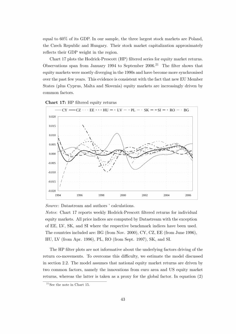
Chart 17 plots the Hodrick-Prescott (HP) filtered series for equity market returns.

Observations span from January 1994 to September 2006.21 The filter shows that

equity markets were mostly diverging in the 1990s and have become more synchronised

over the past few years. This evidence is consistent with the fact that new EUMember

States (plus Cyprus, Malta and Slovenia) equity markets are increasingly driven by

common factors.

Chart 17: HP filtered equity returns

-0.020

-0.015

-0.010

-0.005

0.000

0.005

0.010

0.015

0.020

1994 1996 1998 2000 2002 2004 2006

CY CZ EE HU LV PL SK SI RO BG

Source: Datastream and authors ’ calculations.

Notes: Chart 17 reports weekly Hodrick-Prescott filtered returns for individual

equity markets. All price indices are computed by Datastream with the exception

of EE, LV, SK, and SI where the respective benchmark indices have been used.

The countries included are: BG (from Nov. 2000), CY, CZ, EE (from June 1996),

HU, LV (from Apr. 1996), PL, RO (from Sept. 1997), SK, and SI.

The HP filter plots are not informative about the underlying factors driving of the

return co-movements. To overcome this difficulty, we estimate the model discussed

in section 2.2. The model assumes that national equity market returns are driven by

two common factors, namely the innovations from euro area and US equity market

returns, whereas the latter is taken as a proxy for the global factor. In equation (2)

21See the note in Chart 15.

43

we allow for time-varying “beta” coefficients, which capture the exposure of national

markets to the common factors. The idea is that as economic and financial integration

increases over time, the importance of national factors should decrease. This in turn

implies that the amount of variance explained by euro area and global factors should

increase.

The “beta” coefficients are made time-varying using time dummies as follows:

βEUi,t = ξ0,i+ ξ1,iD1,t+ ξ2,iD2,t. A similar specification is used for the exposure to US

shocks. The dummies (D1,t and D2,t) identify three subperiods, from the beginning of

the sample to October 2001, from November 2001 to April 2004, and from May 2004

to the end of the sample. The choice of dates reflects important economic events. In

November 2001 the future accession of new Member States to the EU was announced,

while in May 2004 the accession actually took place.

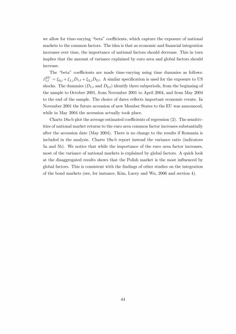
Charts 18a-b plot the average estimated coefficients of regression (2). The sensitiv-

ities of national market returns to the euro area common factor increases substantially

after the accession date (May 2004). There is no change to the results if Romania is

included in the analysis. Charts 19a-b report instead the variance ratio (indicators

5a and 5b). We notice that while the importance of the euro area factor increases,

most of the variance of national markets is explained by global factors. A quick look

at the disaggregated results shows that the Polish market is the most influenced by

global factors. This is consistent with the findings of other studies on the integration

of the bond markets (see, for instance, Kim, Lucey and Wu, 2006 and section 4).

44

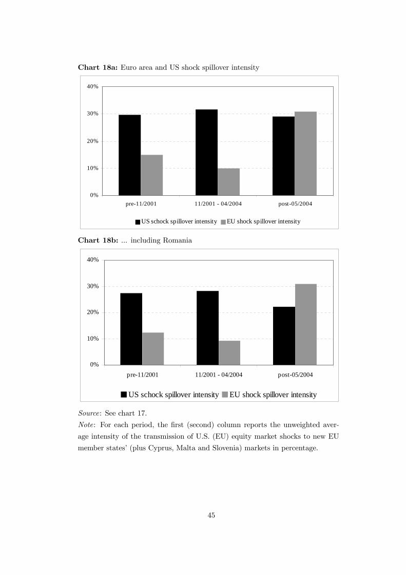
Chart 18a: Euro area and US shock spillover intensity

0%

10%

20%

30%

40%

pre-11/2001 11/2001 - 04/2004 post-05/2004

US schock spillover intensity EU shock spillover intensity

Chart 18b: ... including Romania

0%

10%

20%

30%

40%

pre-11/2001 11/2001 - 04/2004 post-05/2004

US schock spillover intensity EU shock spillover intensity

Source: See chart 17.

Note: For each period, the first (second) column reports the unweighted aver-

age intensity of the transmission of U.S. (EU) equity market shocks to new EU

member states’ (plus Cyprus, Malta and Slovenia) markets in percentage.

45

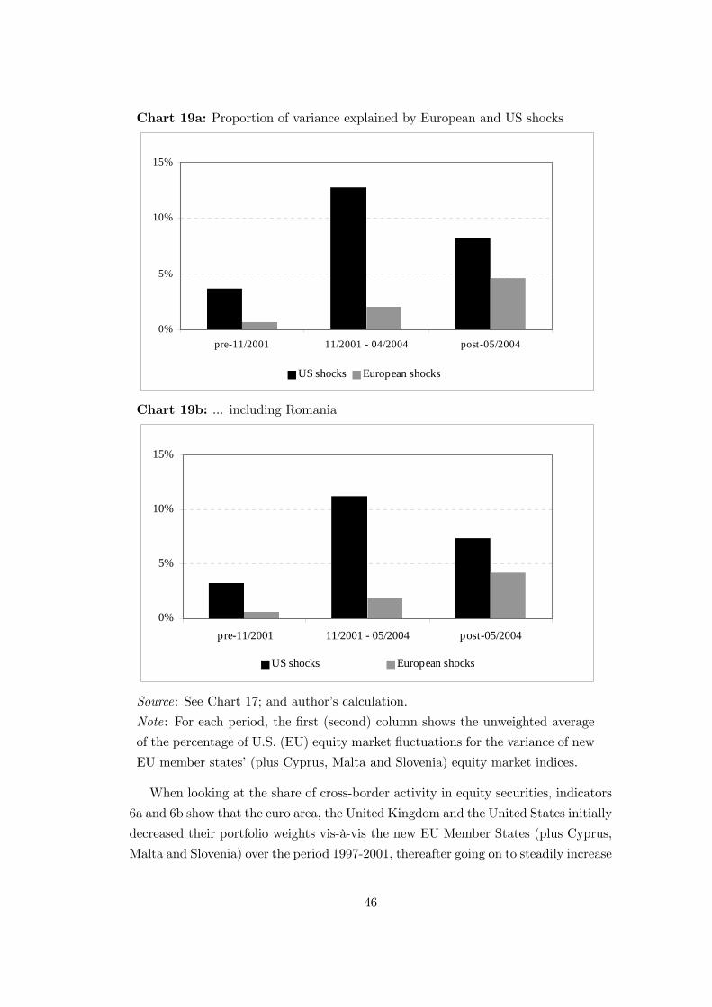
Chart 19a: Proportion of variance explained by European and US shocks

0%

5%

10%

15%

pre-11/2001 11/2001 - 04/2004 post-05/2004

US shocks European shocks

Chart 19b: ... including Romania

0%

5%

10%

15%

pre-11/2001 11/2001 - 05/2004 post-05/2004

US shocks European shocks

Source: See Chart 17; and author’s calculation.

Note: For each period, the first (second) column shows the unweighted average

of the percentage of U.S. (EU) equity market fluctuations for the variance of new

EU member states’ (plus Cyprus, Malta and Slovenia) equity market indices.

When looking at the share of cross-border activity in equity securities, indicators

6a and 6b show that the euro area, the United Kingdom and the United States initially

decreased their portfolio weights vis-à-vis the new EU Member States (plus Cyprus,

Malta and Slovenia) over the period 1997-2001, thereafter going on to steadily increase

46

them (see chart 20 and first five columns of table 5).22 This is a global trend that

is not specific to euro area countries and new EU Member States. Since 2002 most

developing countries have been receiving equity inflows from developed economies.

Therefore, these figures do not signal an increase in integration that is specific to

Europe.

Chart 20: The degree of equity securities issued by new EU Member States (plus

Cyprus, Malta and Slovenia) and held by euro area

0.0%

0.1%

0.2%

0.3%

0.4%

0.5%

0.6%

0.7%

Euro area International Portfolio Euro area Total Portfolio

1997 2001 2002 2003 2004

Source: IMF, Datastream and authors’ calculations.

Note: Euro area’ holdings of foreign equities issued by new EU Member States

(plus Cyprus, Malta and Slovenia) as a share of euro area total foreign holdings

and total portfolio (in percentage).

22The initial decrease is likely to be due to the financial market turbulences which occured between

1997 and 2001 (Asian-Latin American-Russian crises and the burst of the dotcom bubble).

47

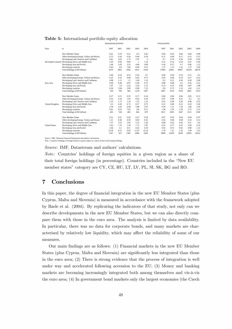
Table 5: International portfolio equity allocationInternational portfolio Total portfolio

from to 1997 2001 2002 2003 2004 1997 2001 2002 2003 2004

New Member States 0.41 0.19 0.31 0.3 0.42 0.06 0.03 0.06 0.06 0.09Other developing Europe, Turkey and Russia 0.75 0.34 0.54 0.64 0.59 0.11 0.06 0.11 0.13 0.13Developing Latin America and Caribbean 4.81 2.03 1.73 1.87 2 0.7 0.34 0.34 0.39 0.45

Developed countriesDeveloping Africa and Middle East 1.02 0.82 0.96 1 1.16 0.15 0.14 0.19 0.21 0.26Developing Asia and Pacific 2.46 3.43 3.53 4.68 4.99 0.36 0.57 0.7 0.96 1.12Developing countries 9.45 6.8 7.06 8.49 9.15 1.37 1.13 1.41 1.75 2.05Total holdings (USD billion) 2470 3662 3592 5015 6340 17085 22061 18047 24339 28270

New Member States 0.49 0.24 0.53 0.56 0.7 0.06 0.04 0.16 0.15 0.2Other developing Europe, Turkey and Russia 0.25 0.33 0.48 0.63 0.77 0.03 0.06 0.14 0.17 0.22Developing Latin America and Caribbean 4.08 1.11 1.2 1.06 1.32 0.5 0.21 0.36 0.28 0.38

Euro area Developing Africa and Middle East 0.69 0.46 0.67 0.58 0.75 0.08 0.08 0.2 0.16 0.22Developing Asia and Pacific 1.07 1.8 2.22 3.24 3.72 0.13 0.33 0.66 0.87 1.08Developing countries 6.59 3.94 5.09 6.08 7.25 0.8 0.73 1.52 1.62 2.11Total holdings (USD billion) 328 700 966 1229 1607 2687 3765 3239 4601 5523

New Member States 0.27 0.21 0.19 0.17 0.34 0.06 0.06 0.06 0.05 0.12Other developing Europe, Turkey and Russia 0.32 0.34 1.03 0.63 0.59 0.07 0.09 0.31 0.2 0.2Developing Latin America and Caribbean 2.33 1.73 1.19 1.55 1.52 0.53 0.48 0.36 0.48 0.52

United Kingdom Developing Africa and Middle East 0.5 0.29 0.73 0.57 0.75 0.12 0.08 0.22 0.18 0.26Developing Asia and Pacific 2.59 4.35 4.48 5.88 5.97 0.59 1.21 1.34 1.84 2.05Developing countries 6.01 6.91 7.62 8.8 9.17 1.38 1.93 2.28 2.75 3.15Total holdings (USD billion) 462 558 493 664 879 2011 2003 1647 2125 2560

New Member States 0.51 0.21 0.29 0.27 0.39 0.07 0.03 0.04 0.04 0.07Other developing Europe, Turkey and Russia 1.21 0.44 0.59 0.83 0.65 0.16 0.06 0.08 0.14 0.12Developing Latin America and Caribbean 7.37 3.22 2.95 3.12 3.36 0.98 0.42 0.42 0.51 0.6

United States Developing Africa and Middle East 1.63 1.33 1.59 1.72 1.87 0.22 0.17 0.23 0.28 0.33Developing Asia and Pacific 2.64 4.1 4.51 6.02 6.29 0.35 0.53 0.65 0.98 1.12Developing countries 13.36 9.31 9.93 11.97 12.54 1.78 1.21 1.43 1.94 2.23Total holdings (USD billion) 1197 613 1385 2080 2560 8990 12439 9638 12819 14412

Source: IMF, Thomson Financial Datastream and authors' calculationsNote: Countries' holdings of foreign bonds in a given region as a share of their total foreign holdings

Source: IMF, Datastream and authors’ calculations.

Note: Countries’ holdings of foreign equities in a given region as a share of

their total foreign holdings (in percentage). Countries included in the “New EU

member states” category are CY, CZ, HU, LT, LV, PL, SI, SK, BG and RO.

7 Conclusions

In this paper, the degree of financial integration in the new EU Member States (plus

Cyprus, Malta and Slovenia) is measured in accordance with the framework adopted

by Baele et al. (2004). By replicating the indicators of that study, not only can we

describe developments in the new EU Member States, but we can also directly com-

pare them with those in the euro area. The analysis is limited by data availability.

In particular, there was no data for corporate bonds, and many markets are char-

acterised by relatively low liquidity, which may affect the reliability of some of our

measures.

Our main findings are as follows: (1) Financial markets in the new EU Member

States (plus Cyprus, Malta and Slovenia) are significantly less integrated than those

in the euro area; (2) There is strong evidence that the process of integration is well

under way and accelerated following accession to the EU; (3) Money and banking

markets are becoming increasingly integrated both among themselves and vis-à-vis

the euro area; (4) In government bond markets only the largest economies (the Czech

48

Republic, Poland and to a lesser extent Hungary) exibit any signs of integration; and

(5) Equity markets are less integrated, although they are increasingly affected by euro

area shocks.

References

[1] Adam, K., T. Jappelli, A. Mennichini, M. Padula, and M Pagano, 2002,

“Analyse, Compare, and Apply Alternative Indicators and Monitoring Method-

ologies to Measure the Evolution of Capital Market Integration in the European

Union,” European Commission Report.

[2] Adjaouté, K. and J.P. Danthine, 2004, “Equity Returns and Integration: Is

Europe Changing?,” Oxford Review of Economic Policy 20(4): 555-570.

[3] Allen, F., L. Bartiloro and O. Kowalewski, 2005, “The Financial System of the

EU 25,” mimeo.

[4] Baele, L., A. Ferrando, P. Hördahl, E. Krylova and C. Monnet, 2004, “Measur-

ing Financial Integration in the Euro Area,” Oxford Review of Economic Policy

20(4): 509-530.

[5] Baklaci, H.-F., 2003, “International government bond markets: determinants of

yields and volatility linkages,” Diss. University of Texas, Arlington.

[6] Brixi, H., P.H. Ghanem and R. Islam, 1999, “Fiscal Adjustment and Contin-

gent Government Liabilities: Case Study of the Czech Republic and Macedonia,”

World Bank Policy Research Paper 2177, Whashington DC.

[7] Byström, H., 2006, “Cross-Sectional Correlation: New Evidence on Changing

Correlations and Correlation Breakdown in Equity Markets,” Global Business

and Finance Review 11(1): 13-28.

[8] Cabral I., F. Dierick and J. Vesala, 2002, “Banking Integration in the Euro Area,”

ECB Occasional Paper # 6.

[9] Campbell, J.Y., M. Lettau, B.G. Malkiel, and Y. Xu, 2001, “Have Individual

Stocks Become more Volatile? An Empirical Exploration of Idiosyncratic Risk,”

Journal of Finance 56: 1-43.

[10] Cappiello, L., B. Gérard, A. Kadareja and S. Manganelli, 2006, “Financial Inte-

gration of New EU Member States,” ECB Working Paper # 683.

49

[11] Caviglia, G., G. Krause and C. Thimann, 2002, “Key Features of the Financial

Sectors in EU Accession Countries,” in C. Thimann (ed.), Financial Sectors in

EU Accession Countries, European Central Bank.

[12] De Santis, R.A. and B. Gerard, 2006, “Financial Integration, International Port-

folio Choice and the European Monetary Union,” ECB Working Paper # 626.

[13] Dvorak, T. and C. R. A. Geiregat, 2004, “Are the New and Old EU Countries

Financially Integrated?,” mimeo, Union College, Schenectady, NY.

[14] European Bank for Reconstruction and Developments, 2006, Transition Report

2006: Finance in Transition, London: EBRD.

[15] European Central Bank, 2002, Financial Sectors in EU Accession Countries,

Frankfurt: ECB.

[16] European Central Bank, 2005a, Indicators of Financial Integration in the Euro

Area, Frankfurt: ECB.

[17] European Central Bank, 2005b, The New EU Member States - Convergence and

Stability, Frankfurt: ECB.

[18] European Central Bank, 2005c, Banking Structures in the New EU Member

States, Frankfurt: ECB.

[19] European Central Bank, 2006a, Indicators of Financial Integration in the Euro

Area, Frankfurt: ECB.

[20] European Central Bank, 2006b, “Financial Development in Central, Eastern and

South-Eastern Europe,” in ECB, Monthly Bulletin, Nov. 2006, 93-103.

[21] European Central Bank, 2007, Indicators of Financial Integration in the Euro

Area, Frankfurt: ECB.

[22] Eiling, E. and B. Gerard, 2006, “Dispersion, Equity Returns Correlations and

Market Integration,” mimeo, Tilburg University.

[23] Fink, G., P. Haiss and G. Vuksic, 2004, “Changing importance of financial sectors

for growth from transition to cohesion and European integration,” Europainstitut

Vienna, Working Paper # 58.

[24] Gerard, B., P. Hillion, F. De Roon, and E. Eiling, 2006, “The Structure of Global

Equity Returns: Currency, Industry and Country Effects Revisited,” EFA 2002,

Berlin. Available at SSRN: http://ssrn.com/abstract=302353.

50

[25] Guiso, L., T. Jappelli, M. Padula and M. Pagano, 2005, “Financial Market In-

tegration and Economic Growth in the EU”, Economic Policy 19(40): 523-577.

[26] Hartmann, P., F. Heider, M. Lo Duca, and E. Papaioannou, 2007, “The Role

of Financial Markets and Innovation for Prodcutivity and Growth in Europe,”

ECB Occasional Paper, forthcoming.

[27] Kim, S.-J., B.-M. Lucey and E. Wu, 2006, “Dynamics of bond market integra-

tion between established and accession European Union countries,” Journal of

International Financial Markets, Institutions and Money 16(1): 41-56.

[28] Levine, R. and S. Zervos, 1996, “Stock Markets Development and Long-Run

Growth,” The World Bank Economic Review, 10: 323-339.

[29] Lommatzsch, L.-T. and K. Orlowski, 2006, “Bond yield compression in the coun-

tries convergin to the euro,” William Davidson Institute Working Paper # 799.

[30] Moody’s, 2004, “Mutual benefits of foreign ownership of Central and East Euro-

pean banks,” Special Comment.

[31] Reininger, T., and Walko, Z., 2006, “The Integration of the Czech, Hungarian

and Polish Bond Markets with the Euro Area Bond Markets — A déjà vu of the

Club-Med Convergence Plays?” In: Liebscher, K., J. Christl, P. Mooslechner, D.

Ritzberger-Grünwald (eds.), Financial Development, Integration and Stability,

Edward Elgar, Cheltenham, UK, Nothampton, MA.

[32] Solnik, B. and J. Roulet, 2000, “Dispersion as Cross-Sectional Correlation,” Fi-

nancial Analysts Journal 56(1): 54-61.

[33] Tang, H., E. Zoli and I. Klytchnikova, 2000, “Banking Crisis in Transition Coun-

tries: Fiscal Costs and Related Issues,”World Bank Policy Research Paper 2484,

Whashington DC.

51