Measuring connectivity using mobile sources –Analysis of truck movements between Thai and
regional cities using probe (GPS) data Hiroyuki Miyazaki, Ph.D.1* and Keola Souknilanh 2
1* Asian Institute of Technology / [email protected] Japan External Trade Organization

Rural development for regional connectivity
Less attention because of little production regardless of importance for infrastructure investment
Which connection should be
prioritized for investment?

Technology – Probe data• Time-series trajectory data of individuals with time-stamps and
locations (typically latitudes and longitudes)
Monday Tuesday Wednesday
Thursday Friday Saturday
stay home during weekend?
From Home to Work?
Satellite-based probe data collection
GPS receiver
GPS receiver
GPS receiver
Record positions (latitude/longitude) per seconds/minutes

Seconds frequency GPS logs of taxis in Bangkok
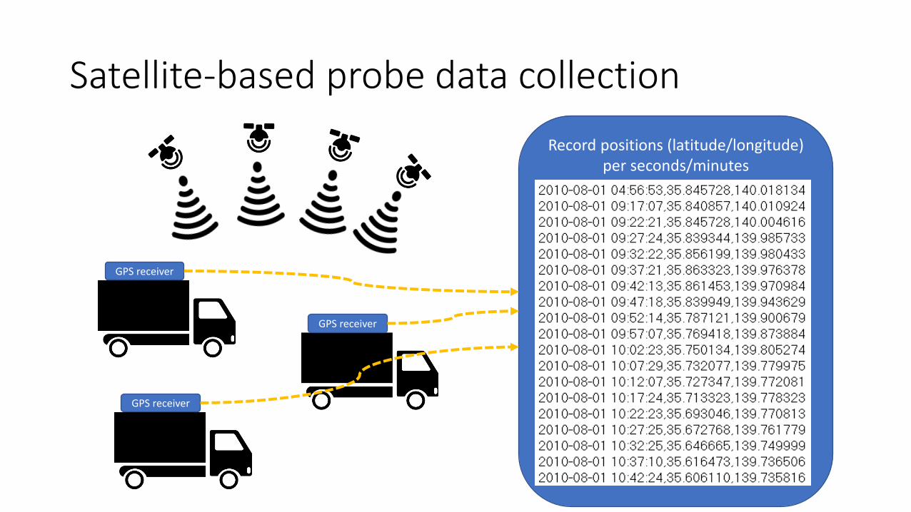
Peungnumsai A, Witayangkurn A, Nagai M, Miyazaki H. A Taxi Zoning Analysis Using Large-Scale Probe Data: A Case Study for Metropolitan Bangkok. The Review of SocionetworkStrategies. 2018 ;12:21-45.
OD analysis of the occupied trips interacting between each administrative zone
Origin point cluster distribution
Preliminary zone generated by origin point distribution
Taxi service zone analysis using the probe data

Mobile Phone Call Detail Records (CDR)
data
data
Data on time and location (base station) of
voice/messaging/data communication of each
hand-set for billing purposes. Data is recorded
only when calling, messaging and data
communication.

CDR in Dhaka

2015.08.26Shibasaki & Sekimoto Lab. CSIS/IIS/EDITORIA. UTokyo 9
Monitoring people movement for Ebola Control with Mobile Phone Data Analysis
Entire Sierra Leone
Freetown Bo

Freetown( Capital City)
Kenema(Hospital)
Possible epicenter?
Map of Sierra Leone

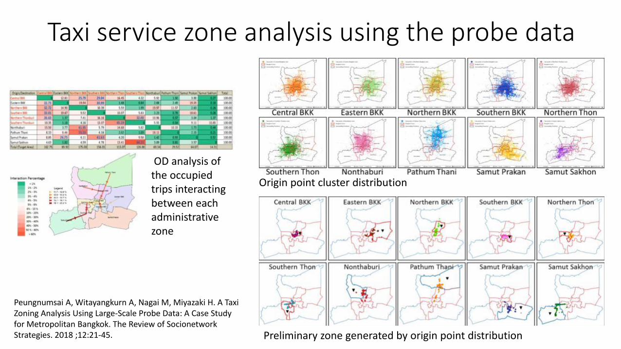
Personal probes from smartphones
Personal probes from smartphones
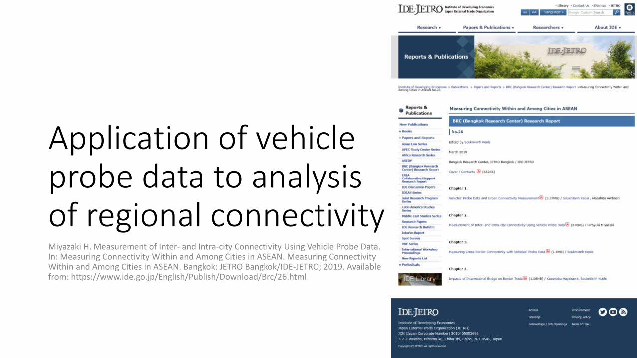
Application of vehicle probe data to analysis of regional connectivityMiyazaki H. Measurement of Inter- and Intra-city Connectivity Using Vehicle Probe Data. In: Measuring Connectivity Within and Among Cities in ASEAN. Measuring Connectivity Within and Among Cities in ASEAN. Bangkok: JETRO Bangkok/IDE-JETRO; 2019. Available from: https://www.ide.go.jp/English/Publish/Download/Brc/26.html
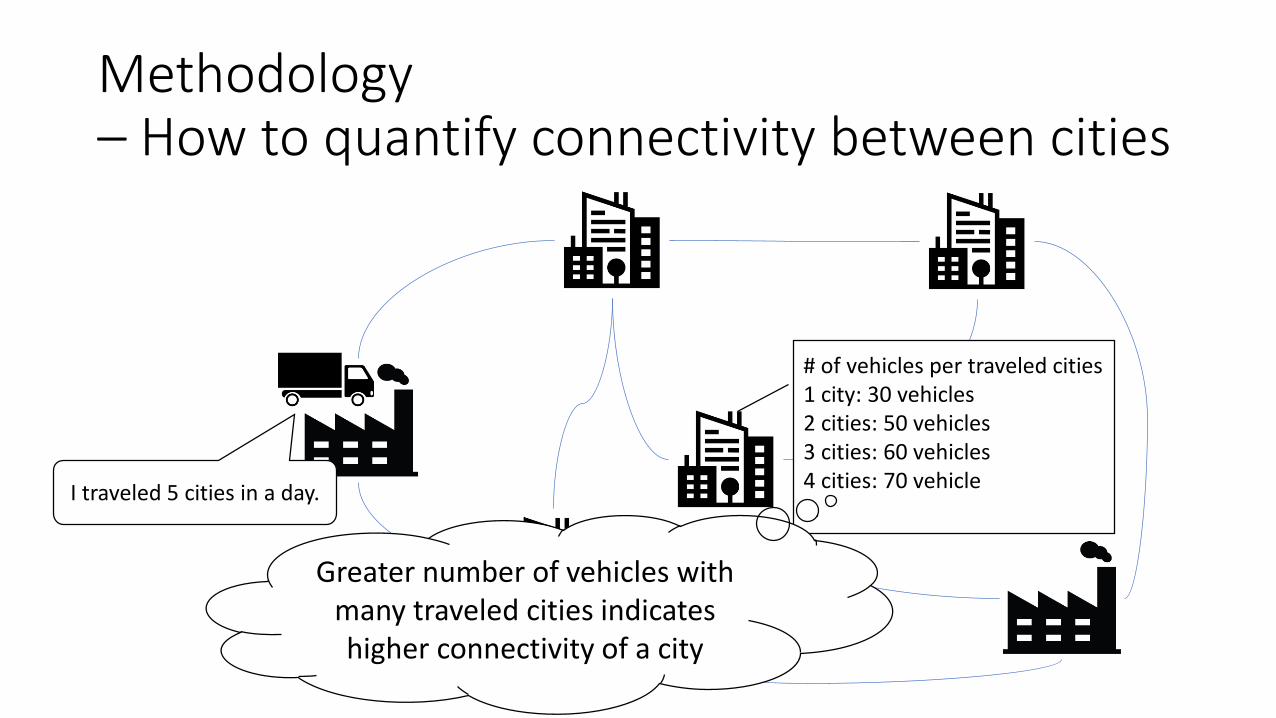
Methodology– How to quantify connectivity between cities
I traveled 5 cities in a day.
# of vehicles per traveled cities1 city: 30 vehicles2 cities: 50 vehicles3 cities: 60 vehicles4 cities: 70 vehicle…
Greater number of vehicles with many traveled cities indicates higher connectivity of a city

Methodology – Overall framework
Intra-city connectivity Inter-city connectivity
Number of vehicles per hour
Average speedper hour
Number of vehicles per number of travelled
cities
More vehicles,better connectivity
Higher speed,better connectivity
More vehicles with many cities traveled, better connectivityTradeoffs in case
of over capacity (to be discussed)

Data and study area
A subset of the GPS logs of commercial vehicles, such as trucks and taxis, collected by Toyota Tsusho Nexty Electronics Thailand.
a) appeared in predefined border areas or
b) appeared in more than two predefined cities
Between
a) 5-6 March 2017
b) 13-14 September2017
c) 4-5 March 2018
d) 12-13 September 2018
The number of records is 140,815,982 in total.
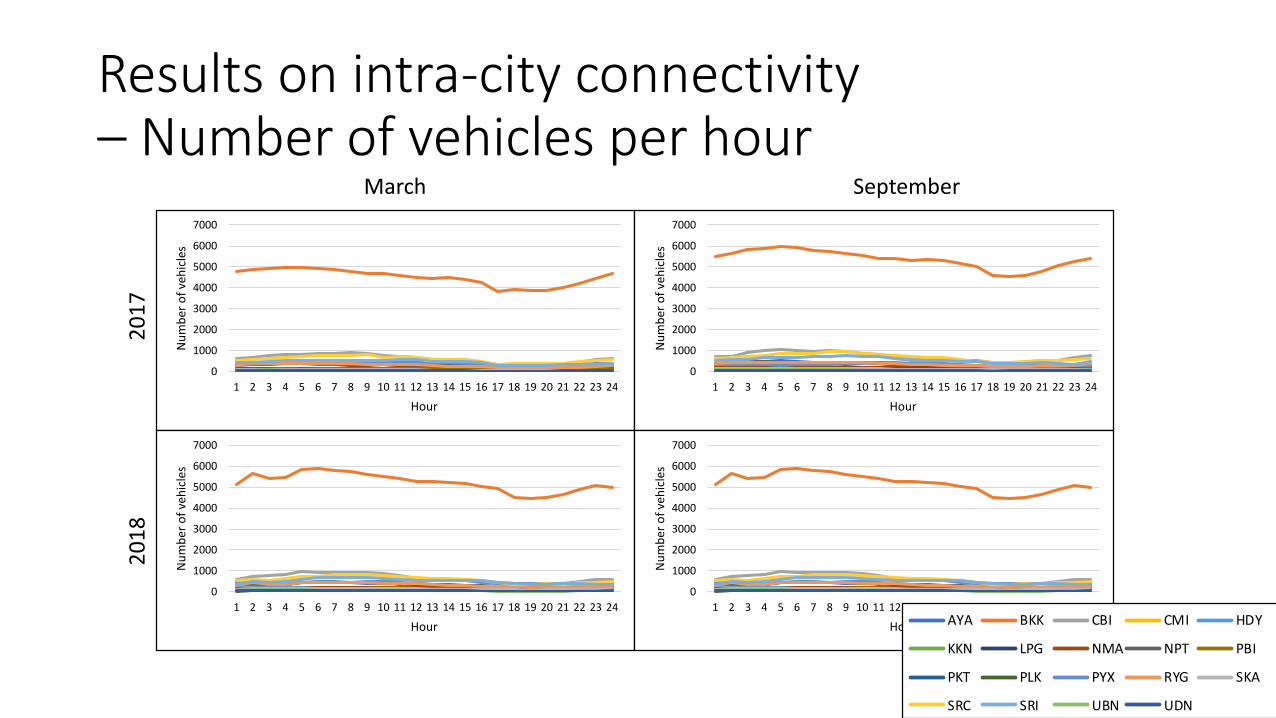
Results on intra-city connectivity– Number of vehicles per hour
0
1000
2000
3000
4000
5000
6000
7000
1 2 3 4 5 6 7 8 9 10 11 12 13 14 15 16 17 18 19 20 21 22 23 24
Nu
mb
er o
f ve
hic
les
Hour
0
1000
2000
3000
4000
5000
6000
7000
1 2 3 4 5 6 7 8 9 10 11 12 13 14 15 16 17 18 19 20 21 22 23 24
Nu
mb
er o
f ve
hic
les
Hour
20
17
0
1000
2000
3000
4000
5000
6000
7000
1 2 3 4 5 6 7 8 9 10 11 12 13 14 15 16 17 18 19 20 21 22 23 24
Nu
mb
er o
f ve
hic
les
Hour
March
0
1000
2000
3000
4000
5000
6000
7000
1 2 3 4 5 6 7 8 9 10 11 12 13 14 15 16 17 18 19 20 21 22 23 24
Nu
mb
er o
f ve
hic
les
Hour
September
0
1000
2000
3000
4000
5000
6000
1 2 3 4 5 6 7 8 9 10 11 12 13 14 15 16 17 18 19 20 21 22 23 24
Nu
mb
er o
f ve
hic
les
Hour
AYA BKK CBI CMI HDY
KKN LPG NMA NPT PBI
PKT PLK PYX RYG SKA
SRC SRI UBN UDN
20
18

Results on intra-city connectivity– Number of vehicles per hour w/o BKK
0
500
1000
1500
2000
1 2 3 4 5 6 7 8 9 10 11 12 13 14 15 16 17 18 19 20 21 22 23 24
Nu
mb
er o
f ve
hic
les
Hour
0
500
1000
1500
2000
1 2 3 4 5 6 7 8 9 10 11 12 13 14 15 16 17 18 19 20 21 22 23 24
Nu
mb
er o
f ve
hic
les
Hour
0
500
1000
1500
2000
1 2 3 4 5 6 7 8 9 10 11 12 13 14 15 16 17 18 19 20 21 22 23 24
Nu
mb
er o
f ve
hic
les
Hour
0
500
1000
1500
2000
1 2 3 4 5 6 7 8 9 10 11 12 13 14 15 16 17 18 19 20 21 22 23 24
Nu
mb
er o
f ve
hic
les
Hour
0
100
200
300
400
500
600
700
800
900
1000
1 2 3 4 5 6 7 8 9 10 11 12 13 14 15 16 17 18 19 20 21 22 23 24
Nu
mb
er o
f ve
hic
les
Hour
AYA CBI CMI HDY KKN LPG
NMA NPT PBI PKT PLK PYX
RYG SKA SRC SRI UBN UDN
March September
20
17
20
18
a) More vehicles in the daytime: KKN, NMA, PBI, PKT, PLK, PYX, RYG, SRC, SRI, UDNb) More vehicles in the night time: AYA, BKK, CBI, CMI, HDY, LPG, NPT, SKA, UBN→ Commercial vehicles are likely avoid heavy traffic in daytime.c) Greater number of vehicles in Sept 2018.
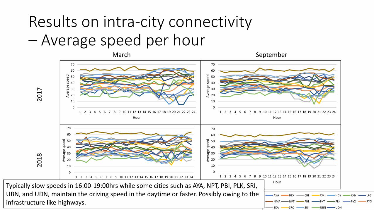
Results on intra-city connectivity– Average speed per hour
0
10
20
30
40
50
60
70
1 2 3 4 5 6 7 8 9 10 11 12 13 14 15 16 17 18 19 20 21 22 23 24
Ave
rage
sp
eed
Hour
March September
20
17
20
18
0
10
20
30
40
50
60
70
1 2 3 4 5 6 7 8 9 10 11 12 13 14 15 16 17 18 19 20 21 22 23 24
Ave
rage
sp
eed
Hour
0
10
20
30
40
50
60
70
1 2 3 4 5 6 7 8 9 10 11 12 13 14 15 16 17 18 19 20 21 22 23 24
Ave
rage
sp
eed
Hour
0
10
20
30
40
50
60
70
1 2 3 4 5 6 7 8 9 10 11 12 13 14 15 16 17 18 19 20 21 22 23 24
Ave
rage
sp
eed
Hour
0
10
20
30
40
50
60
70
80
1 2 3 4 5 6 7 8 9 10 11 12 13 14 15 16 17 18 19 20 21 22 23 24
Ave
rage
sp
eed
Hour
AYA BKK CBI CMI HDY KKN LPG
NMA NPT PBI PKT PLK PYX RYG
SKA SRC SRI UBN UDN
Typically slow speeds in 16:00-19:00hrs while some cities such as AYA, NPT, PBI, PLK, SRI, UBN, and UDN, maintain the driving speed in the daytime or faster. Possibly owing to the infrastructure like highways.

Results on inter-city connectivity—Number of vehicles per number of travelled cities
• Very few vehicles traveled more than 5 cities
• Half of vehicles are connecting two cities by shuttle trips
• Vehicles travelling more than 2 cities are possibly passing through the cities. Further investigation is needed.
0% 10% 20% 30% 40% 50% 60% 70% 80% 90% 100%
5-6 Mar. 2017
13-14 Sep. 2017
4-5 Mar. 2018
12-13 Sep. 2018
1 2 3 4 5 6 or more

0% 20% 40% 60% 80% 100%
AYA
BKK
CBI
CMI
HDY
KKN
LPG
NMA
NPT
PBI
PKT
PLK
PYX
RYG
SKA
SRC
SRI
UBN
UDN March
20
17
20
18
0% 20% 40% 60% 80% 100%
AYA
BKK
CBI
CMI
HDY
KKN
LPG
NMA
NPT
PBI
PKT
PLK
PYX
RYG
SKA
SRC
SRI
UBN
UDN
0% 20% 40% 60% 80% 100%
AYA
BKK
CBI
CMI
HDY
KKN
LPG
NMA
NPT
PBI
PKT
PLK
PYX
RYG
SKA
SRC
SRI
UBN
UDN
0% 20% 40% 60% 80% 100%
AYA
BKK
CBI
CMI
HDY
KKN
LPG
NMA
NPT
PBI
PKT
PLK
PYX
RYG
SKA
SRC
SRI
UBN
UDN
0% 20% 40% 60% 80% 100%
AYA
BKK
CBI
CMI
HDY
KKN
LPG
NMA
NPT
PBI
PKT
PLK
PYX
RYG
SKA
SRC
SRI
UBN
UDN
1 2 3 4 5 6 7 8 9 10 11 12
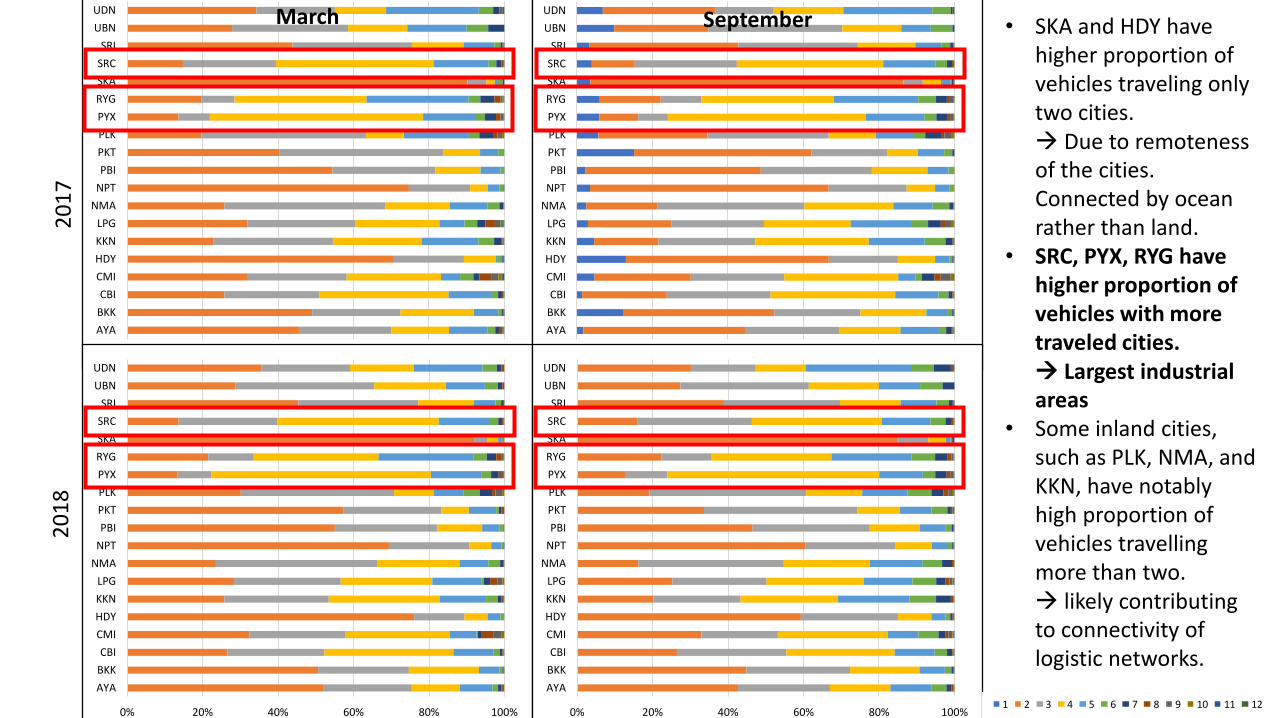
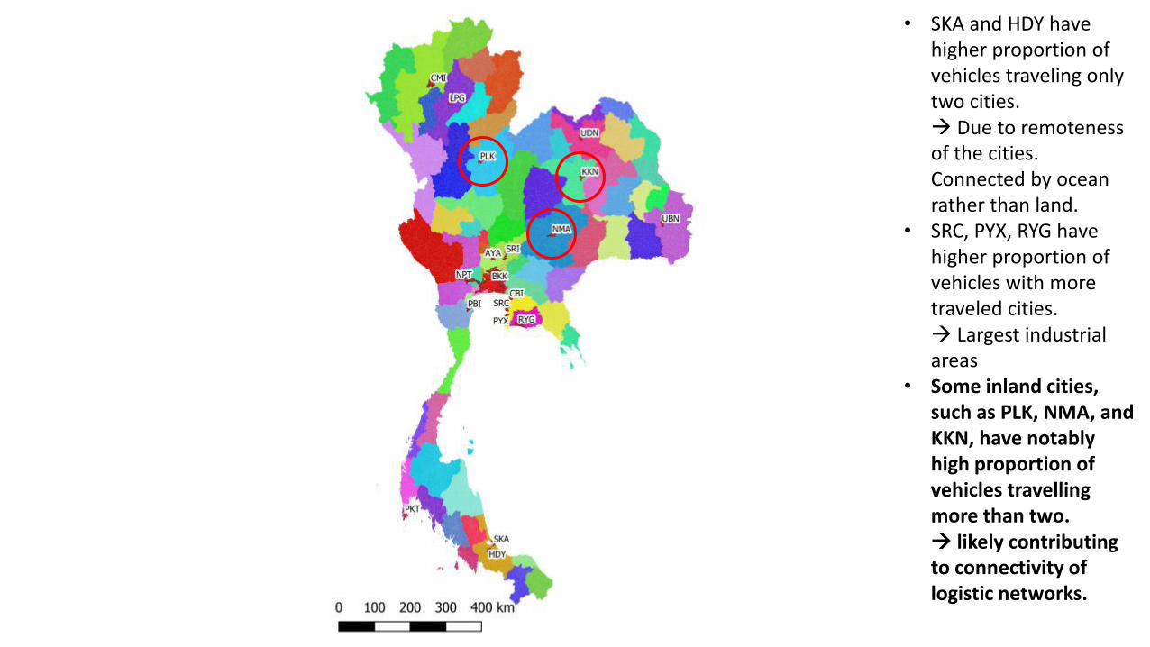
September • SKA and HDY have higher proportion of vehicles traveling only two cities.→ Due to remoteness of the cities. Connected by ocean rather than land.
• SRC, PYX, RYG have higher proportion of vehicles with more traveled cities.→ Largest industrial areas
• Some inland cities, such as PLK, NMA, and KKN, have notably high proportion of vehicles travelling more than two.→ likely contributing to connectivity of logistic networks.

0% 20% 40% 60% 80% 100%
AYA
BKK
CBI
CMI
HDY
KKN
LPG
NMA
NPT
PBI
PKT
PLK
PYX
RYG
SKA
SRC
SRI
UBN
UDN March
20
17
20
18
0% 20% 40% 60% 80% 100%
AYA
BKK
CBI
CMI
HDY
KKN
LPG
NMA
NPT
PBI
PKT
PLK
PYX
RYG
SKA
SRC
SRI
UBN
UDN
0% 20% 40% 60% 80% 100%
AYA
BKK
CBI
CMI
HDY
KKN
LPG
NMA
NPT
PBI
PKT
PLK
PYX
RYG
SKA
SRC
SRI
UBN
UDN
0% 20% 40% 60% 80% 100%
AYA
BKK
CBI
CMI
HDY
KKN
LPG
NMA
NPT
PBI
PKT
PLK
PYX
RYG
SKA
SRC
SRI
UBN
UDN
0% 20% 40% 60% 80% 100%
AYA
BKK
CBI
CMI
HDY
KKN
LPG
NMA
NPT
PBI
PKT
PLK
PYX
RYG
SKA
SRC
SRI
UBN
UDN
1 2 3 4 5 6 7 8 9 10 11 12
September • SKA and HDY have higher proportion of vehicles traveling only two cities.→ Due to remoteness of the cities. Connected by ocean rather than land.
• SRC, PYX, RYG have higher proportion of vehicles with more traveled cities.→ Largest industrial areas
• Some inland cities, such as PLK, NMA, and KKN, have notably high proportion of vehicles travelling more than two.→ likely contributing to connectivity of logistic networks.

• SKA and HDY have higher proportion of vehicles traveling only two cities.→ Due to remoteness of the cities. Connected by ocean rather than land.
• SRC, PYX, RYG have higher proportion of vehicles with more traveled cities.→ Largest industrial areas
• Some inland cities, such as PLK, NMA, and KKN, have notably high proportion of vehicles travelling more than two.→ likely contributing to connectivity of logistic networks.
0% 20% 40% 60% 80% 100%
AYA
BKK
CBI
CMI
HDY
KKN
LPG
NMA
NPT
PBI
PKT
PLK
PYX
RYG
SKA
SRC
SRI
UBN
UDN March
20
17
20
18
0% 20% 40% 60% 80% 100%
AYA
BKK
CBI
CMI
HDY
KKN
LPG
NMA
NPT
PBI
PKT
PLK
PYX
RYG
SKA
SRC
SRI
UBN
UDN
0% 20% 40% 60% 80% 100%
AYA
BKK
CBI
CMI
HDY
KKN
LPG
NMA
NPT
PBI
PKT
PLK
PYX
RYG
SKA
SRC
SRI
UBN
UDN
0% 20% 40% 60% 80% 100%
AYA
BKK
CBI
CMI
HDY
KKN
LPG
NMA
NPT
PBI
PKT
PLK
PYX
RYG
SKA
SRC
SRI
UBN
UDN
0% 20% 40% 60% 80% 100%
AYA
BKK
CBI
CMI
HDY
KKN
LPG
NMA
NPT
PBI
PKT
PLK
PYX
RYG
SKA
SRC
SRI
UBN
UDN
1 2 3 4 5 6 7 8 9 10 11 12
September • SKA and HDY have higher proportion of vehicles traveling only two cities.→ Due to remoteness of the cities. Connected by ocean rather than land.
• SRC, PYX, RYG have higher proportion of vehicles with more traveled cities.→ Largest industrial areas
• Some inland cities, such as PLK, NMA, and KKN, have notably high proportion of vehicles travelling more than two.→ likely contributing to connectivity of logistic networks.

• SKA and HDY have higher proportion of vehicles traveling only two cities.→ Due to remoteness of the cities. Connected by ocean rather than land.
• SRC, PYX, RYG have higher proportion of vehicles with more traveled cities.→ Largest industrial areas
• Some inland cities, such as PLK, NMA, and KKN, have notably high proportion of vehicles travelling more than two.→ likely contributing to connectivity of logistic networks.

0% 20% 40% 60% 80% 100%
AYA
BKK
CBI
CMI
HDY
KKN
LPG
NMA
NPT
PBI
PKT
PLK
PYX
RYG
SKA
SRC
SRI
UBN
UDN March
20
17
20
18
0% 20% 40% 60% 80% 100%
AYA
BKK
CBI
CMI
HDY
KKN
LPG
NMA
NPT
PBI
PKT
PLK
PYX
RYG
SKA
SRC
SRI
UBN
UDN
0% 20% 40% 60% 80% 100%
AYA
BKK
CBI
CMI
HDY
KKN
LPG
NMA
NPT
PBI
PKT
PLK
PYX
RYG
SKA
SRC
SRI
UBN
UDN
0% 20% 40% 60% 80% 100%
AYA
BKK
CBI
CMI
HDY
KKN
LPG
NMA
NPT
PBI
PKT
PLK
PYX
RYG
SKA
SRC
SRI
UBN
UDN
0% 20% 40% 60% 80% 100%
AYA
BKK
CBI
CMI
HDY
KKN
LPG
NMA
NPT
PBI
PKT
PLK
PYX
RYG
SKA
SRC
SRI
UBN
UDN
1 2 3 4 5 6 7 8 9 10 11 12
September • SKA and HDY have higher proportion of vehicles traveling only two cities.→ Due to remoteness of the cities. Connected by ocean rather than land.
• SRC, PYX, RYG have higher proportion of vehicles with more traveled cities.→ Largest industrial areas
• Some inland cities, such as PLK, NMA, and KKN, have notably high proportion of vehicles travelling more than two.→ likely contributing to connectivity of logistic networks.
• SKA and HDY have higher proportion of vehicles traveling only two cities.→ Due to remoteness of the cities. Connected by ocean rather than land.
• SRC, PYX, RYG have higher proportion of vehicles with more traveled cities.→ Largest industrial areas
• Some inland cities, such as PLK, NMA, and KKN, have notably high proportion of vehicles travelling more than two.→ likely contributing to connectivity of logistic networks.

Concluding remarks
• Useful technologies for measuring connectivity• Satellite-based positioning, such as GPS, on vehicles
• Mobile phone call detail records (CDR)
• Personal probes collected by smartphones
• Demonstration of an analysis using probe data application for Thailand• Characterizing the cities in aspects of intra- and inter-city connectivity.
• Cities’ contribution to connectivity were highlighted.
• Remained technical issues• Vehicles’ purposes to drop by a city needs to be investigated. Estimation from stay time in the city.

Measuring connectivity using mobile sources –Analysis of truck movements between Thai and
regional cities using probe (GPS) data Hiroyuki Miyazaki, Ph.D.1* and Keola Souknilanh 2
1* Asian Institute of Technology / [email protected] Japan External Trade Organization
Recommended