MATH/STAT 4720, Life Contingencies IIFall 2017
Toby KenneyIn Class Examples
November 29, 2017 1 / 148

Long-Term Coverages in Health Insurance
Disability Income Insurance (DII)Long-term Care Insurance (LTC)Critical Illness Insurance (CII)Chronic Illness InsuranceHospital Indemnity Insurance (HII)Continuing Care Retirement Communities
November 29, 2017 2 / 148
SN 1.1: Disability Income Insurance
Disability Income InsuranceAlso known as Income Protection InsuranceTypically level premiums while working.Benefits paid during periods of disabilityBenefits based on salary, capped at 50–70% of lost salary.
Features of DIIWaiting period or elimination period is time between start ofdisability and first benefit payment.Total disability benefits paid if policyholder is unable to performtheir usual job (certified by medical practicioner) and is nototherwise employed.Partial disability benefits can be paid if the policyholder cannotwork at full capacity, but is still working.Benefits may be reduced if policyholder has other income.
November 29, 2017 3 / 148
SN 1.1: Disability Income Insurance
Term of DII PaymentsBenefit payment may be limited term or up to retirement age.The term covers both full and partial payments (or a mixture).Limited term payments apply to each period of sickness.Multiple disibilities separated by less than the off period treated asa single disability (for both elimination period and term of benefits).Disability defined either by ability to perform current job, or anyreasonable job given qualifications and experience.Employers may buy as group insurance, receiving cheaper rates.Benefits may increase in line with inflation.Common additional benefit: return to work assistance.
November 29, 2017 4 / 148
SN 1.2 Long Term Care Insurance
Long Term Care InsuranceTypically level premiums while healthy.Typically 90 day waiting period before receiving benefits.Benefits paid when trigger conditions apply
Triggers of LTC (USA and Canada)Trigger usually determined by Activities of Daily Living (ADL)Six commonly used ADLs:
Bathing- Dressing- Eating-Toileting- Continence- Transferring-
Benefit triggered (and waiting period commences) whenpolicyholder is unable to perform two or more of these ADLs.Alternative triggers often based on severe cognitive impairment.Some policies use 3 ADLs as trigger.
November 29, 2017 5 / 148
SN 1.2 Long Term Care Insurance
Other Features of LTC PaymentsBenefits can either be definite term or indefinite term.Benefit may either be reimbursement (up to a limit) or a fixedannuity.Payments or payment limits may increase with inflation.Reimbursed care benefits may be in-home or residential.Hybrid LTC and life insurance. Two approaches:
Return of premium: unused LTC premiums added to death benefit.Accelerated benefits: deducts LTC payments from death benefits.
In the USA, some LTC policies are tax-qualifying.Insurers may reserve the right to increase premiums during thepolicy (subject to regulatory approval).In other countries with government support for LTC costs, LTCinsurance can still be used to top up government support.
November 29, 2017 6 / 148
SN 1.3 Critical Illness Insurance
Critical Illness Insurance (CII)Single lump-sum payout upon diagnosis with any of a prescribedlist of illnesses.Policy expires upon first benefit.Level premiums paid thoughout the term. May stop at a specifiedage.May be incorporated into life insurance as an accelerated benefitrider. Some benefit paid immediately upon diagnosis, remainingbenefit (if any) paid upon death.
November 29, 2017 7 / 148
SN 1.4 Chronic Illness Insurance
Chronic Illness InsuranceLike CII, pays benefit upon diagnosis of one of a number ofconditions.Difference from CII is that conditions are chronic (policyholder willnot recover) but not terminal.Illness must be sufficiently severe that policyholder cannotperform at least 2 ADLs (see LTC section).Benefit paid either as lump sum or as annuity.Typically offered as accelerated benefit rider on life insurancepolicy.
November 29, 2017 8 / 148
SN 1.5 Hospital Indemnity Insurance
Hospital Indemnity Insurance (HII)Lump sum payment for hospitalisation.May include daily stipend for hospital stays.May include additional benefits for outpatient admission.Differs from standard health insurance in that benefits are cashpayments, rather than reimbursement of costs.Premiums increase each year.insurers often guarantee renewal. This means:
Renewal is not subject to medical examination.Future premiums are not affected by claims in earlier years.
November 29, 2017 9 / 148
SN 1.6 Continuing Care Retirement Communities
Continuing Care Retirement Communities (CCRCs)Three or four levels of care offered
Independent Living Unit (ILU) — minimal supportAssisted Living Unit (ALU) — non-medical supportSkilled Nursing Facility (SNF) — ongoing medical careMemory Care Units (MCU) — dementia or cognitive impairments
Variety of funding options:Full life care — large upfront fee & fixed monthly payments.Modified life care — smaller upfront fee & monthly payments.Partially subsidised additional fees for further services.Fee for service — Pay for services as needed.
Full and modified life care options require medical examination.Direct entrants to ALU or SNF only eligible for Fee for service.Full and modified life care packages may include a partial refund ifmore expensive care facilities are not used.Some CCRCs offer partial ownership of the ILU.Joint CCRC membership for couples is common.
November 29, 2017 10 / 148
8 Multiple State Models
“Definition”A Multiple State model has several different states into whichindividuals can be classified. These typically represent differentpayouts made under the policy.
November 29, 2017 11 / 148
8.2 Examples of Multiple State Models
Examples of Multiple State ModelsAlive-Dead.Insurance with Increased Benefit for Accidental DeathPermanent Disability Model.Disability Income Insurance Model
November 29, 2017 12 / 148
8.2 Examples of Multiple State Models
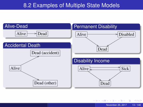
Alive-DeadAlive // Dead
Accidental DeathDead (accident)
Alive
77ooooooooooo
''OOOOO
OOOOOO
Dead (other)
Permanent Disability
Alive //
$$III
IIII
IIDisabled
yyssssss
ssss
Dead
Disability Income
Alive //
$$III
IIII
IISick
{{vvvvvvvvv
oo
Dead
November 29, 2017 13 / 148
8.4 Assumption and Notation
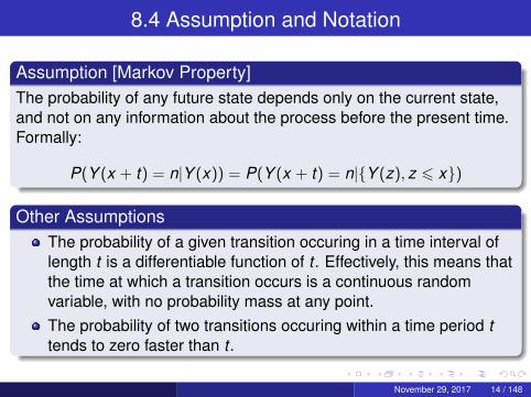
Assumption [Markov Property]The probability of any future state depends only on the current state,and not on any information about the process before the present time.Formally:
P(Y (x + t) = n|Y (x)) = P(Y (x + t) = n|{Y (z), z 6 x})
Other AssumptionsThe probability of a given transition occuring in a time interval oflength t is a differentiable function of t . Effectively, this means thatthe time at which a transition occurs is a continuous randomvariable, with no probability mass at any point.The probability of two transitions occuring within a time period ttends to zero faster than t .
November 29, 2017 14 / 148
Notation and Formulae
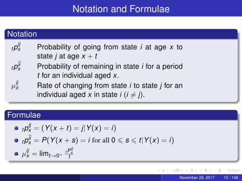
Notation
tpijx Probability of going from state i at age x to
state j at age x + t
tpiix Probability of remaining in state i for a period
t for an individual aged x .µij
x Rate of changing from state i to state j for anindividual aged x in state i (i 6= j).
Formulae
tpijx = (Y (x + t) = j |Y (x) = i)
tpiix = P(Y (x + s) = i for all 0 6 s 6 t |Y (x) = i)
µijx = limt→0+
t Pijx
t
November 29, 2017 15 / 148
8.4 Formulae for Probabilities
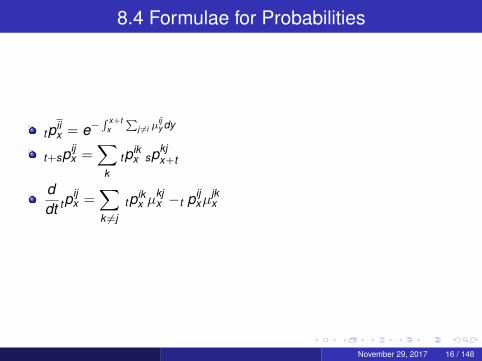
tpiix = e−
∫ x+tx
∑j 6=i µ
ijy dy
t+spijx =
∑k
tpikx spkj
x+t
ddt tp
ijx =
∑k 6=j
tpikx µ
kjx −t pij
xµjkx
November 29, 2017 16 / 148
8.5 Numerical Evaluation of Probabilities
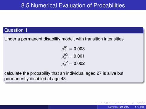
Question 1
Under a permanent disability model, with transition intensities
µ01x = 0.003
µ02x = 0.001
µ12x = 0.002
calculate the probability that an individual aged 27 is alive butpermanently disabled at age 43.
November 29, 2017 17 / 148
8.5 Numerical Evaluation of Probabilities
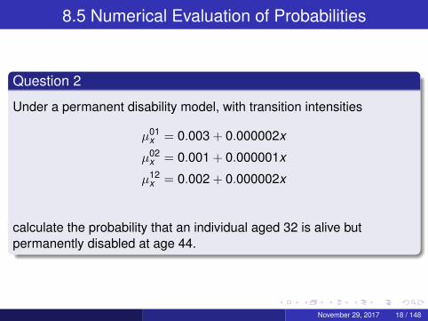
Question 2
Under a permanent disability model, with transition intensities
µ01x = 0.003 + 0.000002x
µ02x = 0.001 + 0.000001x
µ12x = 0.002 + 0.000002x
calculate the probability that an individual aged 32 is alive butpermanently disabled at age 44.
November 29, 2017 18 / 148
8.5 Numerical Evaluation of Probabilities
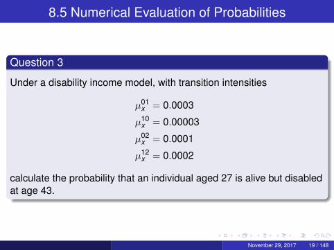
Question 3
Under a disability income model, with transition intensities
µ01x = 0.0003
µ10x = 0.00003
µ02x = 0.0001
µ12x = 0.0002
calculate the probability that an individual aged 27 is alive but disabledat age 43.
November 29, 2017 19 / 148
8.5 Numerical Evaluation of Probabilities
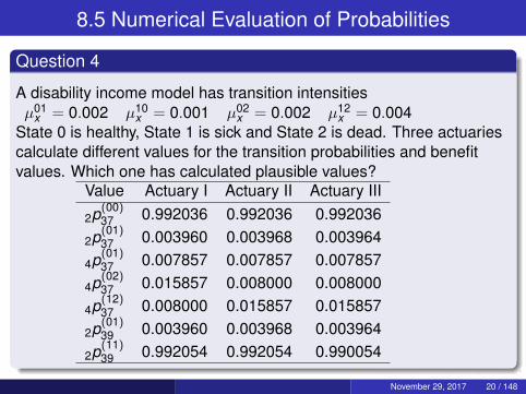
Question 4
A disability income model has transition intensitiesµ01
x = 0.002 µ10x = 0.001 µ02
x = 0.002 µ12x = 0.004
State 0 is healthy, State 1 is sick and State 2 is dead. Three actuariescalculate different values for the transition probabilities and benefitvalues. Which one has calculated plausible values?
Value Actuary I Actuary II Actuary III
2p(00)37 0.992036 0.992036 0.992036
2p(01)37 0.003960 0.003968 0.003964
4p(01)37 0.007857 0.007857 0.007857
4p(02)37 0.015857 0.008000 0.008000
4p(12)37 0.008000 0.015857 0.015857
2p(01)39 0.003960 0.003968 0.003964
2p(11)39 0.992054 0.992054 0.990054
November 29, 2017 20 / 148
8.6 Premiums
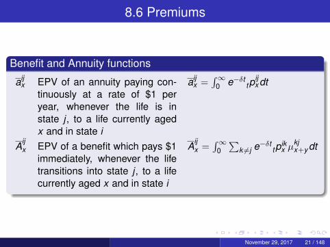
Benefit and Annuity functions
aijx EPV of an annuity paying con-
tinuously at a rate of $1 peryear, whenever the life is instate j , to a life currently agedx and in state i
aijx =
∫∞0 e−δt tp
ijxdt
Aijx EPV of a benefit which pays $1
immediately, whenever the lifetransitions into state j , to a lifecurrently aged x and in state i
Aijx =
∫∞0∑
k 6=j e−δt tpikx µ
kjx+ydt
November 29, 2017 21 / 148
8.6 Premiums
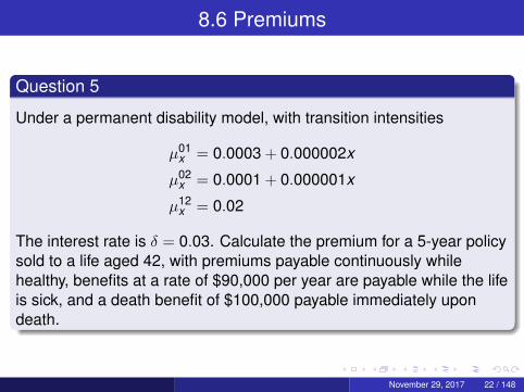
Question 5
Under a permanent disability model, with transition intensities
µ01x = 0.0003 + 0.000002x
µ02x = 0.0001 + 0.000001x
µ12x = 0.02
The interest rate is δ = 0.03. Calculate the premium for a 5-year policysold to a life aged 42, with premiums payable continuously whilehealthy, benefits at a rate of $90,000 per year are payable while the lifeis sick, and a death benefit of $100,000 payable immediately upondeath.
November 29, 2017 22 / 148
8.6 Premiums
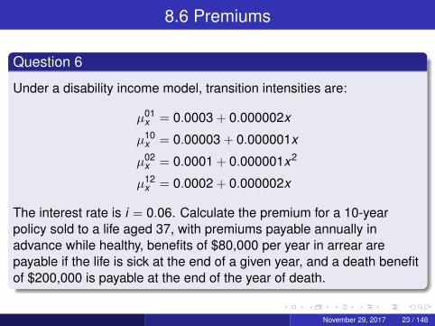
Question 6
Under a disability income model, transition intensities are:
µ01x = 0.0003 + 0.000002x
µ10x = 0.00003 + 0.000001x
µ02x = 0.0001 + 0.000001x2
µ12x = 0.0002 + 0.000002x
The interest rate is i = 0.06. Calculate the premium for a 10-yearpolicy sold to a life aged 37, with premiums payable annually inadvance while healthy, benefits of $80,000 per year in arrear arepayable if the life is sick at the end of a given year, and a death benefitof $200,000 is payable at the end of the year of death.
November 29, 2017 23 / 148
8.6 Premiums
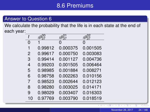
Answer to Question 6We calculate the probability that the life is in each state at the end ofeach year:
t tp0037 tp01
37 tp0237
0 1 0 01 0.99812 0.000375 0.0015052 0.99617 0.000750 0.0030833 0.99414 0.001127 0.0047364 0.99203 0.001505 0.0064645 0.98985 0.001884 0.0082716 0.98758 0.002263 0.0101567 0.98523 0.002644 0.0121238 0.98280 0.003025 0.0141719 0.98029 0.003407 0.01630310 0.97769 0.003790 0.018519
November 29, 2017 24 / 148
8.6 Premiums
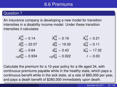
Question 7
An insurance company is developing a new model for transitionintensities in a disability income model. Under these transitionintensities it calculates
A0234 = 0.14 A
0244 = 0.19 A
1244 = 0.21
a0034 = 22.07 a00
44 = 19.30 a1044 = 0.11
a0134 = 0.64 a01
44 = 0.43 a1144 = 17.32
10p0034 = 0.934 10p01
34 = 0.022 δ = 0.03
Calculate the premium for a 10-year policy for a life aged 34, withcontinuous premiums payable while in the healthy state, which pays acontinuous benefit while in the sick state, at a rate of $80,000 per year,and pays a death benefit of $280,000 immediately upon death.
November 29, 2017 25 / 148
8.6 Premiums
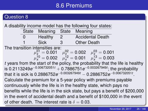
Question 8
A disability income model has the following four states:State Meaning State Meaning0 Healthy 2 Accidental Death1 Sick 3 Other Death
The transition intensities are:µ01
x = 0.001 µ02x = 0.002 µ03
x = 0.001µ10
x = 0.002 µ12x = 0.001 µ13
x = 0.003t years from the start of the policy, the probability that the life is healthyis 0.2113249e−0.006732051t + 0.7886751e−0.003267949t ; the probabilitythat it is sick is 0.2886752e−0.003267949t − 0.2886752e−0.006732051t .Calculate the premium for a 5-year policy with premiums payablecontinuously while the life is in the healthy state, which pays nobenefits while the life is in the sick state, but pays a benefit of $200,000in the event of accidental death and a benefit of $100,000 in the eventof other death. The interest rate is δ = 0.03.
November 29, 2017 26 / 148

8.6 Premiums
Question 9
(a) How does the premium in Question 8 change if there is a waitingperiod of 3 months but no off period for the sick state?(b) How does the premium in Question 8 change if there is a waitingperiod of 3 months and an off period of 6 months for the sick state?
November 29, 2017 27 / 148
8.7 Policy Values and Thiele’s Differential Equation
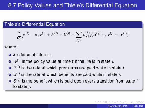
Thiele’s Differential Equationddt t
v (i) = δ tv (i) + P(i) − B(i) −∑j 6=i
µ(ij)x+t (S
(ij) +t v (j) −t v (i))
where:
δ is force of interest.
tv (i) is the policy value at time t if the life is in state i .P(i) is the rate at which premiums are paid while in state i .B(i) is the rate at which benefits are paid while in state i .S(ij) is the benefit which is paid upon every transition from state ito state j .
November 29, 2017 28 / 148
8.7 Policy Values and Thiele’s Differential Equation
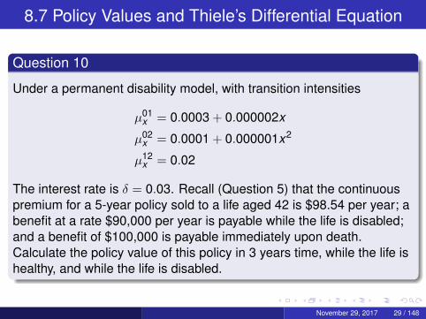
Question 10
Under a permanent disability model, with transition intensities
µ01x = 0.0003 + 0.000002x
µ02x = 0.0001 + 0.000001x2
µ12x = 0.02
The interest rate is δ = 0.03. Recall (Question 5) that the continuouspremium for a 5-year policy sold to a life aged 42 is $98.54 per year; abenefit at a rate $90,000 per year is payable while the life is disabled;and a benefit of $100,000 is payable immediately upon death.Calculate the policy value of this policy in 3 years time, while the life ishealthy, and while the life is disabled.
November 29, 2017 29 / 148
8.7 Policy Values and Thiele’s Differential Equation
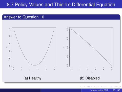
Answer to Question 10
0 1 2 3 4 5
−10
0−
80−
60−
40−
200
t
V
0 1 2 3 4 5
0e+
001e
+05
2e+
053e
+05
4e+
05
t
V
(a) Healthy (b) Disabled
November 29, 2017 30 / 148
8.8 Multiple Decrement Models
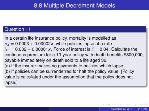
Question 11
In a certain life insurance policy, mortality is modelled asµx = 0.0003 + 0.00002x , while policies lapse at a rateλx = 0.002− 0.00001x . Force of interest is δ = 0.04. Calculate thecontinuous premium for a 10-year policy with death benefits $300,000,payable immediately on death sold to a life aged 36.(a) If the insurer makes no payments to policies which lapse.(b) If policies can be surrenderred for half the policy value. [Policyvalue is calculated under the assumption that the policy does notlapse.]
November 29, 2017 31 / 148
8.8 Multiple Decrement Models
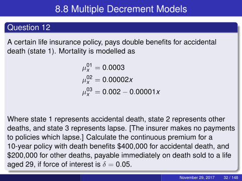
Question 12
A certain life insurance policy, pays double benefits for accidentaldeath (state 1). Mortality is modelled as
µ01x = 0.0003
µ02x = 0.00002x
µ03x = 0.002− 0.00001x
Where state 1 represents accidental death, state 2 represents otherdeaths, and state 3 represents lapse. [The insurer makes no paymentsto policies which lapse.] Calculate the continuous premium for a10-year policy with death benefits $400,000 for accidental death, and$200,000 for other deaths, payable immediately on death sold to a lifeaged 29, if force of interest is δ = 0.05.
November 29, 2017 32 / 148
8.9 Multiple Decrement Tables
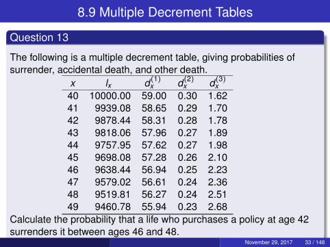
Question 13
The following is a multiple decrement table, giving probabilities ofsurrender, accidental death, and other death.
x lx d (1)x d (2)
x d (3)x
40 10000.00 59.00 0.30 1.6241 9939.08 58.65 0.29 1.7042 9878.44 58.31 0.28 1.7843 9818.06 57.96 0.27 1.8944 9757.95 57.62 0.27 1.9845 9698.08 57.28 0.26 2.1046 9638.44 56.94 0.25 2.2347 9579.02 56.61 0.24 2.3648 9519.81 56.27 0.24 2.5149 9460.78 55.94 0.23 2.68
Calculate the probability that a life who purchases a policy at age 42surrenders it between ages 46 and 48.
November 29, 2017 33 / 148
8.9 Multiple Decrement Tables
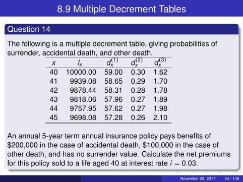
Question 14
The following is a multiple decrement table, giving probabilities ofsurrender, accidental death, and other death.
x lx d (1)x d (2)
x d (3)x
40 10000.00 59.00 0.30 1.6241 9939.08 58.65 0.29 1.7042 9878.44 58.31 0.28 1.7843 9818.06 57.96 0.27 1.8944 9757.95 57.62 0.27 1.9845 9698.08 57.28 0.26 2.10
An annual 5-year term annual insurance policy pays benefits of$200,000 in the case of accidental death, $100,000 in the case ofother death, and has no surrender value. Calculate the net premiumsfor this policy sold to a life aged 40 at interest rate i = 0.03.
November 29, 2017 34 / 148
8.9 Multiple Decrement Tables
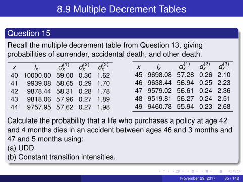
Question 15Recall the multiple decrement table from Question 13, givingprobabilities of surrender, accidental death, and other death.
x lx d (1)x d (2)
x d (3)x
40 10000.00 59.00 0.30 1.6241 9939.08 58.65 0.29 1.7042 9878.44 58.31 0.28 1.7843 9818.06 57.96 0.27 1.8944 9757.95 57.62 0.27 1.98
x lx d (1)x d (2)
x d (3)x
45 9698.08 57.28 0.26 2.1046 9638.44 56.94 0.25 2.2347 9579.02 56.61 0.24 2.3648 9519.81 56.27 0.24 2.5149 9460.78 55.94 0.23 2.68
Calculate the probability that a life who purchases a policy at age 42and 4 months dies in an accident between ages 46 and 3 months and47 and 5 months using:(a) UDD(b) Constant transition intensities.
November 29, 2017 35 / 148
8.10 Constructing a Multiple Decrement Table
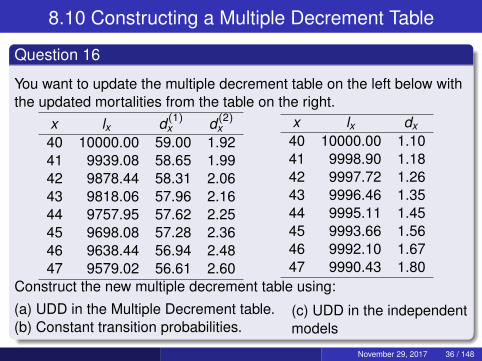
Question 16
You want to update the multiple decrement table on the left below withthe updated mortalities from the table on the right.
x lx d (1)x d (2)
x40 10000.00 59.00 1.9241 9939.08 58.65 1.9942 9878.44 58.31 2.0643 9818.06 57.96 2.1644 9757.95 57.62 2.2545 9698.08 57.28 2.3646 9638.44 56.94 2.4847 9579.02 56.61 2.60
x lx dx40 10000.00 1.1041 9998.90 1.1842 9997.72 1.2643 9996.46 1.3544 9995.11 1.4545 9993.66 1.5646 9992.10 1.6747 9990.43 1.80
Construct the new multiple decrement table using:
(a) UDD in the Multiple Decrement table.(b) Constant transition probabilities.
(c) UDD in the independentmodels
November 29, 2017 36 / 148
8.10 Constructing a Multiple Decrement Table
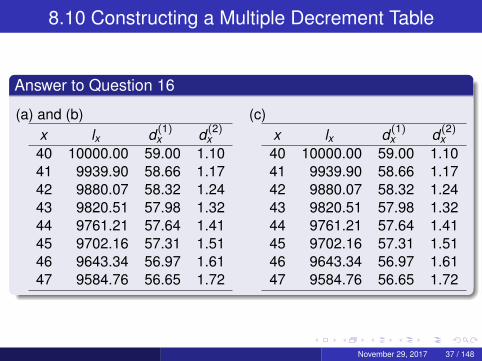
Answer to Question 16
(a) and (b)x lx d (1)
x d (2)x
40 10000.00 59.00 1.1041 9939.90 58.66 1.1742 9880.07 58.32 1.2443 9820.51 57.98 1.3244 9761.21 57.64 1.4145 9702.16 57.31 1.5146 9643.34 56.97 1.6147 9584.76 56.65 1.72
(c)x lx d (1)
x d (2)x
40 10000.00 59.00 1.1041 9939.90 58.66 1.1742 9880.07 58.32 1.2443 9820.51 57.98 1.3244 9761.21 57.64 1.4145 9702.16 57.31 1.5146 9643.34 56.97 1.6147 9584.76 56.65 1.72
November 29, 2017 37 / 148
9.2 Joint Life and Last Survivor Benefits
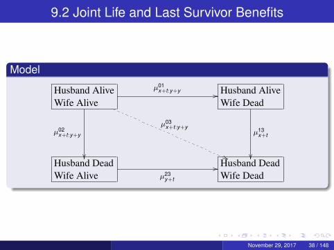
Model
Husband AliveWife Alive
µ01x+t :y+y //
µ03x+t :y+y
((
µ02x+t :y+y
��
Husband AliveWife Dead
µ13x+t
��Husband DeadWife Alive µ23
y+t
// Husband DeadWife Dead
November 29, 2017 38 / 148
9.2 Joint Life and Last Survivor Benefits
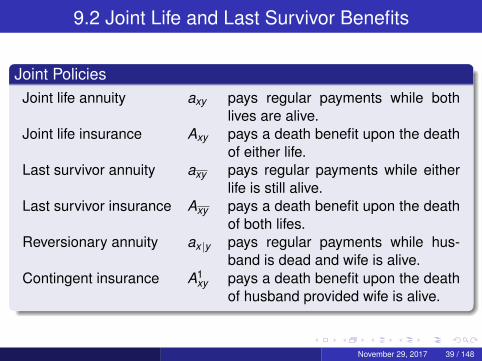
Joint PoliciesJoint life annuity axy pays regular payments while both
lives are alive.Joint life insurance Axy pays a death benefit upon the death
of either life.Last survivor annuity axy pays regular payments while either
life is still alive.Last survivor insurance Axy pays a death benefit upon the death
of both lifes.Reversionary annuity ax |y pays regular payments while hus-
band is dead and wife is alive.Contingent insurance A1
xy pays a death benefit upon the deathof husband provided wife is alive.
November 29, 2017 39 / 148
9.2 Joint Life and Last Survivor Benefits
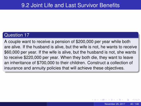
Question 17A couple want to receive a pension of $200,000 per year while bothare alive. If the husband is alive, but the wife is not, he wants to receive$60,000 per year. If the wife is alive, but the husband is not, she wantsto receive $220,000 per year. When they both die, they want to leavean inheritance of $700,000 to their children. Construct a collection ofinsurance and annuity policies that will achieve these objectives.
November 29, 2017 40 / 148

9.2 Joint Life and Last Survivor Benefits
Question 18
What are the advantages and disadvantages of a reversionary annuityover a standard life insurance policy, whose benefit could be used topurchase an annuity at the time the life dies.
November 29, 2017 41 / 148
9.2 Joint Life and Last Survivor Benefits
Formulae
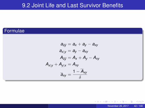
axy = ax + ay − axy
ax |y = ay − axy
Axy = Ax + Ay − Axy
Ax |y + Ay |x = Axy
axy =1− Axy
δ
November 29, 2017 42 / 148
9.2 Joint Life and Last Survivor Benefits
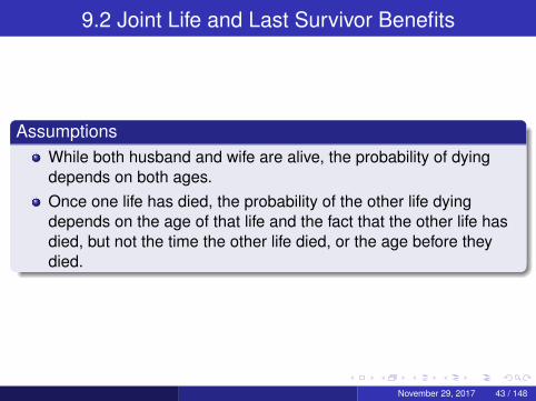
AssumptionsWhile both husband and wife are alive, the probability of dyingdepends on both ages.Once one life has died, the probability of the other life dyingdepends on the age of that life and the fact that the other life hasdied, but not the time the other life died, or the age before theydied.
November 29, 2017 43 / 148
9.3 Joint Life Notation
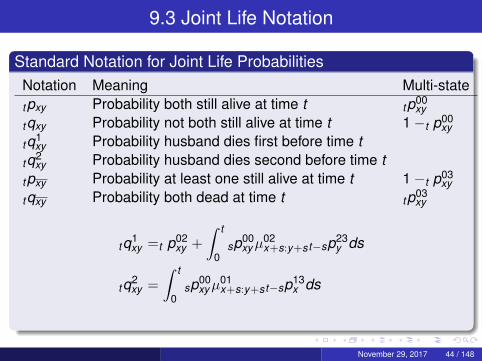
Standard Notation for Joint Life ProbabilitiesNotation Meaning Multi-statetpxy Probability both still alive at time t tp00
xy
tqxy Probability not both still alive at time t 1−t p00xy
tq1xy Probability husband dies first before time t
tq2xy Probability husband dies second before time t
tpxy Probability at least one still alive at time t 1−t p03xy
tqxy Probability both dead at time t tp03xy
tq1xy =t p02
xy +
∫ t
0sp00
xyµ02x+s:y+st−sp23
y ds
tq2xy =
∫ t
0sp00
xyµ01x+s:y+st−sp13
x ds
November 29, 2017 44 / 148

9.3 Joint Life Notation
Formulae
axy =
∫ ∞0
e−δt tp00xy dt
Axy =
∫ ∞0
e−δt tp00xy (µ01
x+t :y+t + µ02x+t :y+t )dt
axy =
∫ ∞0
e−δt (tp00xy +t p01
xy +t p02xy )dt
Axy =
∫ ∞0
e−δt (tp00xyµ
03x+t :y+t +t p01
xyµ13x+t +t p02
xyµ23y+t )dt
ax |y =
∫ ∞0
e−δt tp02xy dt
A1xy =
∫ ∞0
e−δt tp00xyµ
02x+t :y+tdt
November 29, 2017 45 / 148
9.4 Independent Future Lifetimes
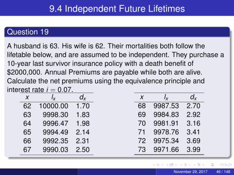
Question 19
A husband is 63. His wife is 62. Their mortalities both follow thelifetable below, and are assumed to be independent. They purchase a10-year last survivor insurance policy with a death benefit of$2000,000. Annual Premiums are payable while both are alive.Calculate the net premiums using the equivalence principle andinterest rate i = 0.07.
x lx dx62 10000.00 1.7063 9998.30 1.8364 9996.47 1.9865 9994.49 2.1466 9992.35 2.3167 9990.03 2.50
x lx dx68 9987.53 2.7069 9984.83 2.9270 9981.91 3.1671 9978.76 3.4172 9975.34 3.6973 9971.66 3.99
November 29, 2017 46 / 148
9.4 Independent Future Lifetimes
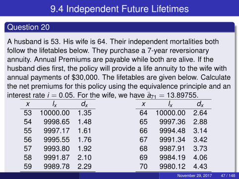
Question 20
A husband is 53. His wife is 64. Their independent mortalities bothfollow the lifetables below. They purchase a 7-year reversionaryannuity. Annual Premiums are payable while both are alive. If thehusband dies first, the policy will provide a life annuity to the wife withannual payments of $30,000. The lifetables are given below. Calculatethe net premiums for this policy using the equivalence principle and aninterest rate i = 0.05. For the wife, we have a71 = 13.89755.
x lx dx53 10000.00 1.3554 9998.65 1.4855 9997.17 1.6156 9995.55 1.7657 9993.80 1.9258 9991.87 2.1059 9989.78 2.29
x lx dx64 10000.00 2.6465 9997.36 2.8866 9994.48 3.1467 9991.34 3.4268 9987.91 3.7369 9984.19 4.0670 9980.12 4.43
November 29, 2017 47 / 148
9.4 Independent Future Lifetimes
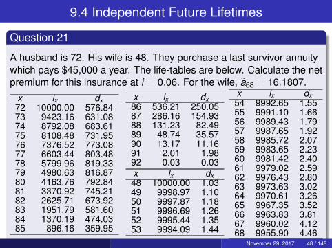
Question 21
A husband is 72. His wife is 48. They purchase a last survivor annuitywhich pays $45,000 a year. The life-tables are below. Calculate the netpremium for this insurance at i = 0.06. For the wife, a68 = 16.1807.
x lx dx72 10000.00 576.8473 9423.16 631.0874 8792.08 683.6175 8108.48 731.9576 7376.52 773.0877 6603.44 803.4878 5799.96 819.3379 4980.63 816.8780 4163.76 792.8481 3370.92 745.2182 2625.71 673.9283 1951.79 581.6084 1370.19 474.0385 896.16 359.95
x lx dx86 536.21 250.0587 286.16 154.9388 131.23 82.4989 48.74 35.5790 13.17 11.1691 2.01 1.9892 0.03 0.03x lx dx48 10000.00 1.0349 9998.97 1.1050 9997.87 1.1851 9996.69 1.2652 9995.44 1.3553 9994.09 1.44
x lx dx54 9992.65 1.5555 9991.10 1.6656 9989.43 1.7957 9987.65 1.9258 9985.72 2.0759 9983.65 2.2360 9981.42 2.4061 9979.02 2.5962 9976.43 2.8063 9973.63 3.0264 9970.61 3.2665 9967.35 3.5266 9963.83 3.8167 9960.02 4.1268 9955.90 4.46
November 29, 2017 48 / 148
9.4 Independent Future Lifetimes
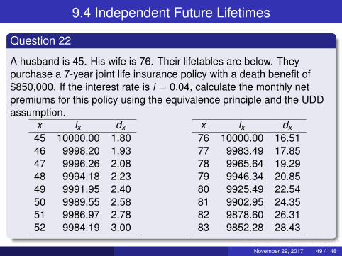
Question 22
A husband is 45. His wife is 76. Their lifetables are below. Theypurchase a 7-year joint life insurance policy with a death benefit of$850,000. If the interest rate is i = 0.04, calculate the monthly netpremiums for this policy using the equivalence principle and the UDDassumption.
x lx dx45 10000.00 1.8046 9998.20 1.9347 9996.26 2.0848 9994.18 2.2349 9991.95 2.4050 9989.55 2.5851 9986.97 2.7852 9984.19 3.00
x lx dx76 10000.00 16.5177 9983.49 17.8578 9965.64 19.2979 9946.34 20.8580 9925.49 22.5481 9902.95 24.3582 9878.60 26.3183 9852.28 28.43
November 29, 2017 49 / 148
9.6 A Model with Dependent Future Lifetimes
Why are joint lives not independent?Broken heart syndrome.Common accident or illness.Similar lifestyles.
November 29, 2017 50 / 148
9.6 A Model with Dependent Future Lifetimes
Question 23
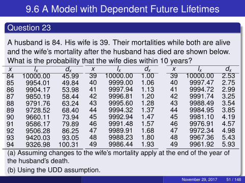
A husband is 84. His wife is 39. Their mortalities while both are aliveand the wife’s mortality after the husband has died are shown below.What is the probability that the wife dies within 10 years?x lx dx84 10000.00 45.9985 9954.01 49.8486 9904.17 53.9887 9850.19 58.4488 9791.76 63.2489 9728.52 68.4090 9660.11 73.9491 9586.17 79.8992 9506.28 86.2593 9420.03 93.0594 9326.98 100.31
x lx dx39 10000.00 1.0040 9999.00 1.0641 9997.94 1.1342 9996.81 1.2043 9995.60 1.2844 9994.32 1.3745 9992.94 1.4746 9991.48 1.5747 9989.91 1.6848 9988.23 1.8049 9986.44 1.93
x lx dx39 10000.00 2.5340 9997.47 2.7541 9994.72 2.9942 9991.74 3.2543 9988.49 3.5444 9984.95 3.8545 9981.10 4.1946 9976.91 4.5747 9972.34 4.9848 9967.36 5.4349 9961.92 5.93
(a) Assuming changes to the wife’s mortality apply at the end of the year ofthe husband’s death.(b) Using the UDD assumption.
November 29, 2017 51 / 148
9.6 A Model with Dependent Future Lifetimes
Question 24
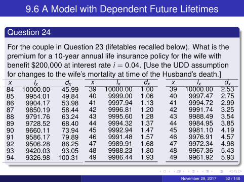
For the couple in Question 23 (lifetables recalled below). What is thepremium for a 10-year annual life insurance policy for the wife withbenefit $200,000 at interest rate i = 0.04. [Use the UDD assumptionfor changes to the wife’s mortality at time of the Husband’s death.]x lx dx84 10000.00 45.9985 9954.01 49.8486 9904.17 53.9887 9850.19 58.4488 9791.76 63.2489 9728.52 68.4090 9660.11 73.9491 9586.17 79.8992 9506.28 86.2593 9420.03 93.0594 9326.98 100.31
x lx dx39 10000.00 1.0040 9999.00 1.0641 9997.94 1.1342 9996.81 1.2043 9995.60 1.2844 9994.32 1.3745 9992.94 1.4746 9991.48 1.5747 9989.91 1.6848 9988.23 1.8049 9986.44 1.93
x lx dx39 10000.00 2.5340 9997.47 2.7541 9994.72 2.9942 9991.74 3.2543 9988.49 3.5444 9984.95 3.8545 9981.10 4.1946 9976.91 4.5747 9972.34 4.9848 9967.36 5.4349 9961.92 5.93
November 29, 2017 52 / 148
9.7 The Common Shock Model
Question 25
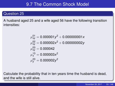
A husband aged 25 and a wife aged 56 have the following transitionintensities:
µ01xy = 0.000001y2 + 0.000000001x
µ02xy = 0.000002x2 + 0.000000002y
µ03xy = 0.000042
µ13x = 0.000003x2
µ23y = 0.000002y2
Calculate the probability that in ten years time the husband is dead,and the wife is still alive.
November 29, 2017 53 / 148
9.7 The Common Shock Model
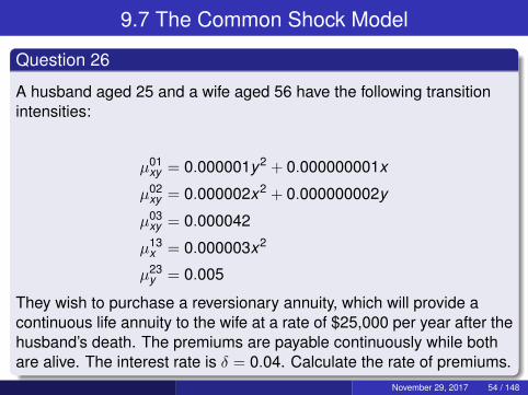
Question 26
A husband aged 25 and a wife aged 56 have the following transitionintensities:
µ01xy = 0.000001y2 + 0.000000001x
µ02xy = 0.000002x2 + 0.000000002y
µ03xy = 0.000042
µ13x = 0.000003x2
µ23y = 0.005
They wish to purchase a reversionary annuity, which will provide acontinuous life annuity to the wife at a rate of $25,000 per year after thehusband’s death. The premiums are payable continuously while bothare alive. The interest rate is δ = 0.04. Calculate the rate of premiums.
November 29, 2017 54 / 148
9.7 The Common Shock Model
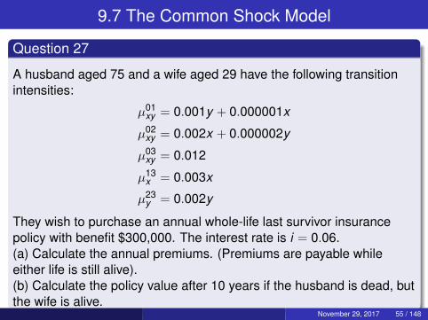
Question 27
A husband aged 75 and a wife aged 29 have the following transitionintensities:
µ01xy = 0.001y + 0.000001x
µ02xy = 0.002x + 0.000002y
µ03xy = 0.012
µ13x = 0.003x
µ23y = 0.002y
They wish to purchase an annual whole-life last survivor insurancepolicy with benefit $300,000. The interest rate is i = 0.06.(a) Calculate the annual premiums. (Premiums are payable whileeither life is still alive).(b) Calculate the policy value after 10 years if the husband is dead, butthe wife is alive.
November 29, 2017 55 / 148
SN 4.1 Mortality Improvement Modelling
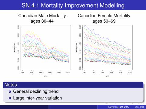
Canadian Male Mortality Canadian Female Mortalityages 30–44 ages 50–69
1960 1970 1980 1990 2000 2010
0.00
00.
001
0.00
20.
003
0.00
40.
005
year
Mor
talit
y R
ates
1960 1970 1980 1990 2000 2010
0.00
00.
005
0.01
00.
015
0.02
00.
025
yearM
orta
lity
Rat
es
NotesGeneral declining trendLarge inter-year variation
November 29, 2017 56 / 148

SN 4.1 Mortality Improvement ModellingCanadian Mortality Improvement
Male Female
1930 1940 1950 1960 1970 1980 1990 2000
3040
5060
7080
90
1930 1940 1950 1960 1970 1980 1990 2000
3040
5060
7080
90
Type of EffectYear effectsAge effectsCohort effects
November 29, 2017 57 / 148

SN 4.1 Mortality Improvement ModellingCanadian Mortality Improvement
Male Female
1930 1940 1950 1960 1970 1980 1990 2000
3040
5060
7080
90
1930 1940 1950 1960 1970 1980 1990 2000
3040
5060
7080
90
Type of EffectYear effectsAge effectsCohort effects
November 29, 2017 57 / 148
SN 4.2 Mortality Improvement Scales
Mortality Improvement ScalesDeterministic function for q(x , t) (Mortality at age x in year t).Generally obtained as product of q(x ,0) and scale function.Simplest are single-factor scale functions depending only on age:q(x , t) = q(x ,0)(1− φx )t
Decreasing mortality increases cost of annuities, increases cost oflife insurance.Longevity risk: risk of losses arising from misestimating futuremortality.More advanced models have improvement factors which are afunction of both age and year.
November 29, 2017 58 / 148
SN 4.2 Mortality Improvement Scales
Constructing Two-Dimensional Improvement ScalesFirst calculate smoothed mortality improvment factors (based onsmoothing log of mortality rate) for existing data.Calculate short term improvement factors from recent experience.Calculate long term improvement factors from whole experience.Decide when short term factors should revert to long term ones.Use smooth interpolation (e.g. cubic functions) to calculateintermediate term improvement factors.
Incorporating Both Age and Cohort EffectsUse the above interpolation method on age groups to get oneimprovement scale.Use the above interpolation method on cohort groups to get oneimprovement scale.Take the average of the two interpolated scales.
November 29, 2017 59 / 148
SN 4.2 Mortality Improvement Scales
Question 28
For males, our smoothed mortality improvment isφ(45,2000) = 0.01863027, ∂φ(x ,t)
∂t
∣∣∣x=45,t=2000
= 0.001077732,
φ(32,2000) = 0.03146243 and dφ(x+t ,t)dt
∣∣∣x=32,t=2000
= 0.001847864.
You decide that the long-term trend is φ(x , t) = 0.01 for all x between30 and 60, and that this trend should be used from 2025 onwards. Usethe interpolation method from the previous slide to calculateφ(45,2013)
November 29, 2017 60 / 148
Stochastic Mortality Scales
Why use Stochastic Mortality ScalesMortality rates have a lot of random fluctuation.Deterministic mortality scales can give good expected presentvalue, but don’t give enough information about the risks.Longevity risks are non-diversifiable. This means the samemortality applies to all policyholders, so it cannot be reduced byselling more policies. (See Chapter 11 of textbook).
November 29, 2017 61 / 148
SN 4.4 The Lee Carter Model
Central Death Rates
mx =qx∫ 1
0 tpx dt=
∫ 10 tpxµx+t dt∫ 1
0 tpx dt
Model
log(m(x , t)) = αx + βxKt + εx ,t
αx and βx depend only on x .Kt depends only on t .Kt is given by a stochastic process Kt = Kt−1 + c + σkZt where Ztare independant standard normal random variables.c and σk are estimated from the data.εx ,t is random fluctuation and is assumed negligible.We add the constraints
∑βx = 1 and
∑Kt = 0.
November 29, 2017 62 / 148
SN 4.4 The Lee Carter Model
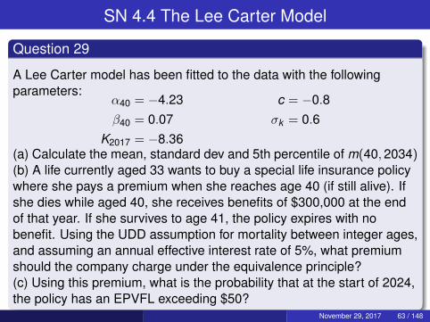
Question 29
A Lee Carter model has been fitted to the data with the followingparameters:
α40 = −4.23 c = −0.8β40 = 0.07 σk = 0.6
K2017 = −8.36(a) Calculate the mean, standard dev and 5th percentile of m(40,2034)(b) A life currently aged 33 wants to buy a special life insurance policywhere she pays a premium when she reaches age 40 (if still alive). Ifshe dies while aged 40, she receives benefits of $300,000 at the endof that year. If she survives to age 41, the policy expires with nobenefit. Using the UDD assumption for mortality between integer ages,and assuming an annual effective interest rate of 5%, what premiumshould the company charge under the equivalence principle?(c) Using this premium, what is the probability that at the start of 2024,the policy has an EPVFL exceeding $50?
November 29, 2017 63 / 148
SN 4.4 The Lee Carter Model
Problems with Lee Carter ModelDoes not fit data well.Does not account for cohort effects.Assumes effects perfectly correlated at different ages.
November 29, 2017 64 / 148
SN 4.5 Cairns-Blake-Dowd Models
Original Model
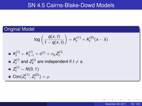
log(
q(x , t)1− q(x , t)
)= K (1)
t + K (2)t (x − x)
K (i)t = K (i)
t−1 + c(i) + σki Z(i)t
Z (i)t and Z (j)
s are independent if t 6= s.
Z (i)t ∼ N(0,1)
Cov(Z (1)t ,Z (2)
t ) = ρ.
November 29, 2017 65 / 148
SN 4.5 Cairns-Blake-Dowd Models
Question 30
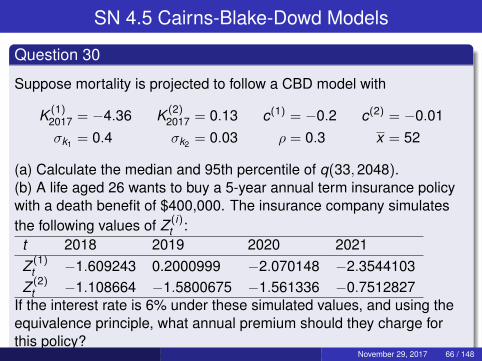
Suppose mortality is projected to follow a CBD model with
K (1)2017 = −4.36 K (2)
2017 = 0.13 c(1) = −0.2 c(2) = −0.01σk1 = 0.4 σk2 = 0.03 ρ = 0.3 x = 52
(a) Calculate the median and 95th percentile of q(33,2048).(b) A life aged 26 wants to buy a 5-year annual term insurance policywith a death benefit of $400,000. The insurance company simulatesthe following values of Z (i)
t :t 2018 2019 2020 2021Z (1)
t −1.609243 0.2000999 −2.070148 −2.3544103Z (2)
t −1.108664 −1.5800675 −1.561336 −0.7512827If the interest rate is 6% under these simulated values, and using theequivalence principle, what annual premium should they charge forthis policy?
November 29, 2017 66 / 148
SN 4.5 Cairns-Blake-Dowd Models
The CBD M7 model
log(
q(x , t)1− q(x , t)
)= K (1)
t + K (2)t (x − x) + K (3)
t ((x − x)2 − sx2) + Gt−x
RemarksFirst two terms are the same as for the original CBD model.Third term adds a quadratic age dependance.Fourth term gives a cohort effect time series. t − x is the year ofbirth of the cohort.Gt−x is usually fitted using an ARIMA model.
November 29, 2017 67 / 148
SN 4.7 Notes on Mortality Improvement Modelling
RemarksTypically use Monte Carlo Simulation to assess longevity risk.For each set of simulated q(x , t) values, we can calculate theactuarial value of annuities and benefits. We therefore get asample of actuarial values.Typically, we take the value for the whole portfolio, becausechanges to mortality are correlated between different age groups.Importance of age, year and cohort effects can vary betweenpopulations.This type of modelling requires a lot of data. It can be difficult tomodel for subpopulations.Policyholders tend to be wealthier and thus have first access toimprovements in mortality.
November 29, 2017 68 / 148
SN 4.7 Notes on Mortality Improvement Modelling
Further RemarksWhole-population models may underestimate longevity risk ifpolicyholder mortality improves faster than the population.Conversely, they may underestimate longevity risk ifimprovements to policyholder mortality slow down before the restof the population.Can generate deterministic scales from mean or median ofstochastic model.Other time series models can be used.Model selection is challenging, there is large parameteruncertainty, and all models fit badly.
November 29, 2017 69 / 148
LM 12.1 The Empirical Distribution
Question 31
Calculate the empirical distribution and cumulative hazard rate functionfor the following data set:
4 3 6 0 3 7 0 0 2 1 1 3 6 3 4
November 29, 2017 70 / 148
LM 12.1 The Empirical Distribution
Question 32
For the data set from the previous question,
4 3 6 0 3 7 0 0 2 1 1 3 6 3 4
compute a Nelson-Åalen estimate for the probability that a randomsample is larger than 5.
November 29, 2017 71 / 148
LM 12.2 The Empirical Distribution for Grouped Data
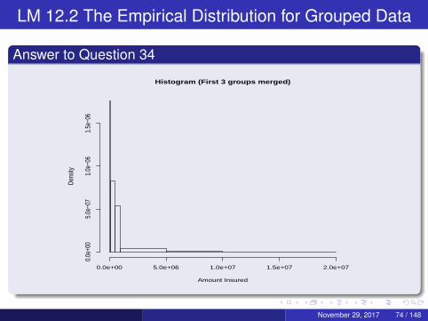
Question 33
An insurance company collects the following data on life insurancepolicies:
Amount Insured Number of PoliciesLess than $5,000 30$5,000–$20,000 52$20,000–$100,000 112$100,000–$500,000 364$500,000–$1,000,000 294$1,000,000–$5,000,000 186$5,000,000–$10,000,000 45More than $10,000,000 16
The government is proposing a tax on insurance policies for amountslarger than $300,000. Using the ogive to estimate the empiricaldistribution function, what is the probability that a random policy isaffected by this tax?
November 29, 2017 72 / 148
LM 12.2 The Empirical Distribution for Grouped Data
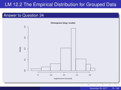
Question 34
Draw the histogram for the data from Question 33
November 29, 2017 73 / 148
LM 12.2 The Empirical Distribution for Grouped Data
Answer to Question 34
Histogram (First 3 groups merged)
Amount Insured
Dens
ity
0.0e+00 5.0e+06 1.0e+07 1.5e+07 2.0e+07
0.0e
+00
5.0e
−07
1.0e
−06
1.5e
−06
November 29, 2017 74 / 148
LM 12.2 The Empirical Distribution for Grouped Data
Answer to Question 34
Histogram (log−scale)
log(Amount Insured)
Dens
ity
8 10 12 14 16
0.0
0.1
0.2
0.3
0.4
November 29, 2017 75 / 148
LM 12.2 The Empirical Distribution for Grouped Data
Question 35
A sample of size 2,000 contains 1,700 observations that are at most6,000; 30 that are between 6,000 and 7,000; and 270 that are morethan 7,000. The total of the 30 observations between 6,000 and 7,000is 200,000. The value of E(X ∧ 6000) under the empirical distributionobtained from this data is 1,810. Calculate the value of E(X ∧ 7000)under the empirical distribution obtained from this data.
November 29, 2017 76 / 148
LM 12.2 The Empirical Distribution for Grouped Data
Question 36
A random sample of unknown size includes 36 observations between 0and 50, x observations between 50 and 150, y observations between150 and 250, 84 observations between 250 and 500, 80 observationsbetween 500 and 1,000, and no observations above 1,000.The ogive includes the values Fn(90) = 0.21 and Fn(210) = 0.51.Calculate x and y .
November 29, 2017 77 / 148
LM 12.2 The Empirical Distribution for Grouped Data
Question 37
Calculate the variance of the empirical survival function for groupeddata using the ogive.
November 29, 2017 78 / 148
LM 12.2 The Empirical Distribution for Grouped Data
Question 38
An insurance company receives 4,356 claims, of which 2,910 are lessthan $10,000, and 763 are between $10,000 and $100,000. Calculatea 95% confidence interval for the probability that a random claim islarger than $50,000.
November 29, 2017 79 / 148
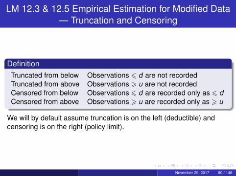
LM 12.3 & 12.5 Empirical Estimation for Modified Data— Truncation and Censoring
DefinitionTruncated from below Observations 6 d are not recordedTruncated from above Observations > u are not recordedCensored from below Observations 6 d are recorded only as 6 dCensored from above Observations > u are recorded only as > u
We will by default assume truncation is on the left (deductible) andcensoring is on the right (policy limit).
November 29, 2017 80 / 148
Example Data Set
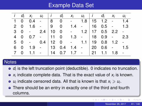
i di xi ui i di xi ui i di xi ui1 0 0.4 - 8 0 - 1.8 15 1.2 - 1.42 0 1.6 - 9 0 1.4 - 16 0.5 - 1.33 0 - 2.4 10 0 - 1.2 17 0.5 2.2 -4 0 0.7 - 11 0 1.3 - 18 0.9 - 2.35 0 - 0.4 12 0 - 1.1 19 0.8 1.2 -6 0 1.9 - 13 0.4 1.4 - 20 0.6 - 1.57 0 1.1 - 14 0.7 1.7 - 21 1.1 1.8 -
Notesdi is the left truncation point (deductible). 0 indicates no truncation.xi indicate complete data. That is the exact value of xi is known.ui indicate censored data. All that is known is that xi > ui .There should be an entry in exactly one of the third and fourthcolumns.
November 29, 2017 81 / 148

Kaplan-Meier Product-Limit Estimator
Notationyj Unique uncensored values sorted in increasing order
y1 < . . . < yksj Number of times yj occurs in the samplerj Size of risk set at yj . That is the number of samples i
such that di < yj < xi or di < yj < ui
Formulaerj = |{i |xi > rj}|+ |{i |ui > rj}| − |{i |di > rj}|rj = |{i |di < rj}| − |{i |ui < rj}| − |{i |xi < rj}|
Kaplan-Meier Product Limit-EstimatorFor yj−1 < t 6 yj :
S(t) =
j−1∏i=1
(1− si
ri
)November 29, 2017 82 / 148
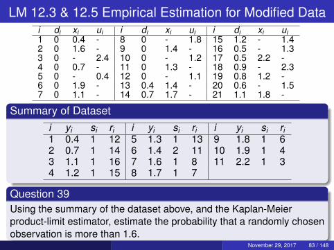
LM 12.3 & 12.5 Empirical Estimation for Modified Datai di xi ui i di xi ui i di xi ui1 0 0.4 - 8 0 - 1.8 15 1.2 - 1.42 0 1.6 - 9 0 1.4 - 16 0.5 - 1.33 0 - 2.4 10 0 - 1.2 17 0.5 2.2 -4 0 0.7 - 11 0 1.3 - 18 0.9 - 2.35 0 - 0.4 12 0 - 1.1 19 0.8 1.2 -6 0 1.9 - 13 0.4 1.4 - 20 0.6 - 1.57 0 1.1 - 14 0.7 1.7 - 21 1.1 1.8 -
Summary of Dataseti yi si ri i yi si ri i yi si ri1 0.4 1 12 5 1.3 1 13 9 1.8 1 62 0.7 1 14 6 1.4 2 11 10 1.9 1 43 1.1 1 16 7 1.6 1 8 11 2.2 1 34 1.2 1 15 8 1.7 1 7
Question 39Using the summary of the dataset above, and the Kaplan-Meierproduct-limit estimator, estimate the probability that a randomly chosenobservation is more than 1.6.
November 29, 2017 83 / 148
LM 12.3 & 12.5 Empirical Estimation for Modified Data
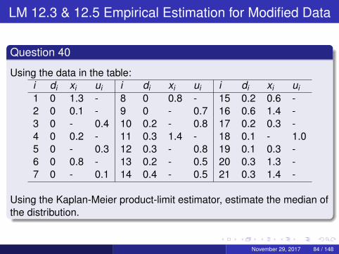
Question 40
Using the data in the table:i di xi ui i di xi ui i di xi ui1 0 1.3 - 8 0 0.8 - 15 0.2 0.6 -2 0 0.1 - 9 0 - 0.7 16 0.6 1.4 -3 0 - 0.4 10 0.2 - 0.8 17 0.2 0.3 -4 0 0.2 - 11 0.3 1.4 - 18 0.1 - 1.05 0 - 0.3 12 0.3 - 0.8 19 0.1 0.3 -6 0 0.8 - 13 0.2 - 0.5 20 0.3 1.3 -7 0 - 0.1 14 0.4 - 0.5 21 0.3 1.4 -
Using the Kaplan-Meier product-limit estimator, estimate the median ofthe distribution.
November 29, 2017 84 / 148
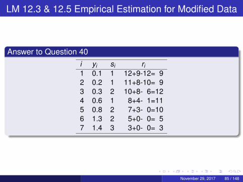
LM 12.3 & 12.5 Empirical Estimation for Modified Data
Answer to Question 40i yi si ri1 0.1 1 12+9-12= 92 0.2 1 11+8-10= 93 0.3 2 10+8- 6=124 0.6 1 8+4- 1=115 0.8 2 7+3- 0=106 1.3 2 5+0- 0= 57 1.4 3 3+0- 0= 3
November 29, 2017 85 / 148
LM 12.3 & 12.5 Empirical Estimation for Modified Data
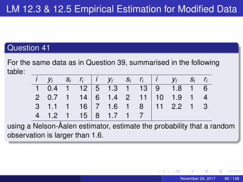
Question 41
For the same data as in Question 39, summarised in the followingtable:
i yi si ri i yi si ri i yi si ri1 0.4 1 12 5 1.3 1 13 9 1.8 1 62 0.7 1 14 6 1.4 2 11 10 1.9 1 43 1.1 1 16 7 1.6 1 8 11 2.2 1 34 1.2 1 15 8 1.7 1 7
using a Nelson-Åalen estimator, estimate the probability that a randomobservation is larger than 1.6.
November 29, 2017 86 / 148
LM 12.3 & 12.5 Empirical Estimation for Modified Data
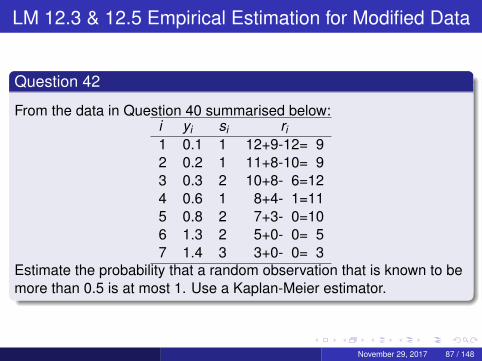
Question 42
From the data in Question 40 summarised below:i yi si ri1 0.1 1 12+9-12= 92 0.2 1 11+8-10= 93 0.3 2 10+8- 6=124 0.6 1 8+4- 1=115 0.8 2 7+3- 0=106 1.3 2 5+0- 0= 57 1.4 3 3+0- 0= 3
Estimate the probability that a random observation that is known to bemore than 0.5 is at most 1. Use a Kaplan-Meier estimator.
November 29, 2017 87 / 148
LM 12.3 & 12.5 Empirical Estimation for Modified Data
Question 43
Show that under the assumption that the sizes of the risk set and thepossible dying times are fixed, the Kaplan-Meier product-limit estimateis unbiassed and calculate its variance.
November 29, 2017 88 / 148
Greenwood’s Approximation
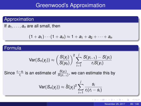
ApproximationIf a1, . . . ,an are all small, then
(1 + a1) · · · (1 + an) ≈ 1 + a1 + a2 + · · ·+ an
Formula
Var(Sn(yj)) ≈(
S(yj)
S(y0)
)2 j∑i=1
S(yi−1)− S(yi)
riS(yi)
Since ri−siri
is an estimate of S(yi )S(yi−1) , we can estimate this by
Var(Sn(yj)) ≈ S(yj)2
j∑i=1
si
ri(ri − si)
November 29, 2017 89 / 148
LM 12.3 & 12.5 Empirical Estimation for Modified Data
Question 44
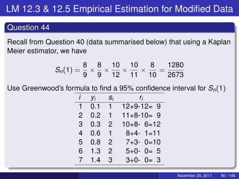
Recall from Question 40 (data summarised below) that using a KaplanMeier estimator, we have
Sn(1) =89× 8
9× 10
12× 10
11× 8
10=
12802673
Use Greenwood’s formula to find a 95% confidence interval for Sn(1)i yi si ri1 0.1 1 12+9-12= 92 0.2 1 11+8-10= 93 0.3 2 10+8- 6=124 0.6 1 8+4- 1=115 0.8 2 7+3- 0=106 1.3 2 5+0- 0= 57 1.4 3 3+0- 0= 3
November 29, 2017 90 / 148
Log-transformed Confidence Interval
ProblemThe usual method for constructing a confidence interval for S(x) maylead to impossible values (negative or more than 1).
SolutionInstead find a confidence interval for
log(− log(S(x)))
which has no impossible values.
November 29, 2017 91 / 148
Log-transformed Confidence Interval (Continued)
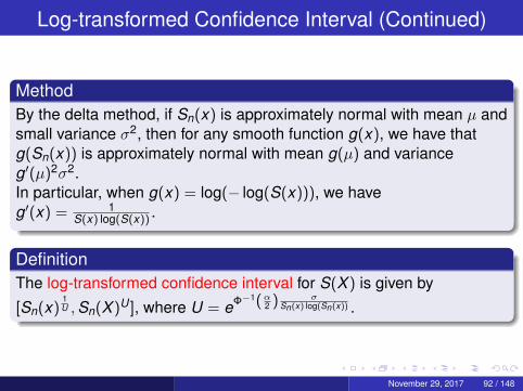
MethodBy the delta method, if Sn(x) is approximately normal with mean µ andsmall variance σ2, then for any smooth function g(x), we have thatg(Sn(x)) is approximately normal with mean g(µ) and varianceg′(µ)2σ2.In particular, when g(x) = log(− log(S(x))), we haveg′(x) = 1
S(x) log(S(x)) .
DefinitionThe log-transformed confidence interval for S(X ) is given by
[Sn(x)1U ,Sn(X )U ], where U = eΦ−1(α
2 ) σSn(x) log(Sn(x)) .
November 29, 2017 92 / 148
LM 12.3 & 12.5 Empirical Estimation for Modified Data
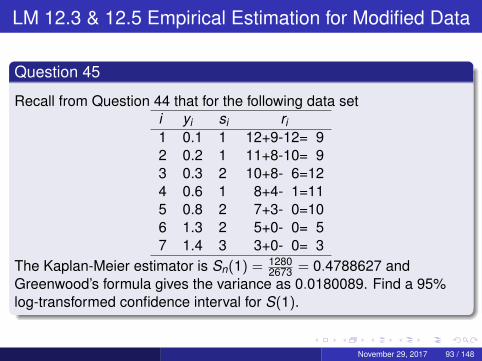
Question 45
Recall from Question 44 that for the following data seti yi si ri1 0.1 1 12+9-12= 92 0.2 1 11+8-10= 93 0.3 2 10+8- 6=124 0.6 1 8+4- 1=115 0.8 2 7+3- 0=106 1.3 2 5+0- 0= 57 1.4 3 3+0- 0= 3
The Kaplan-Meier estimator is Sn(1) = 12802673 = 0.4788627 and
Greenwood’s formula gives the variance as 0.0180089. Find a 95%log-transformed confidence interval for S(1).
November 29, 2017 93 / 148
LM 12.3 & 12.5 Empirical Estimation for Modified Data
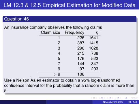
Question 46
An insurance company observes the following claimsClaim size Frequency ri
1 226 16412 387 14153 290 10284 215 7385 176 5237 144 3479 97 203
> 9 106Use a Nelson Åalen estimator to obtain a 95% log-transformedconfidence interval for the probability that a random claim is more than5.
November 29, 2017 94 / 148
LM 12.7 Approximations for Large Data Sets
AimConstruct a lifetable from data in a mortality study. For each individualthis data includes:
Age at entry. (This might either be when the policy was purchasedor when the study started if the policy was purchased before thistime.)Age at exit.Reason for exit (death or other). Other exits might be surrender ortermination of policy or end of study period.
November 29, 2017 95 / 148
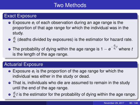
Two Methods
Exact ExposureExposure ei of each observation during an age range is theproportion of that age range for which the individual was in thestudy.diei
(deaths divided by exposures) is the estimator for hazard rate.
The probability of dying within the age range is 1− e−diei
t where tis the length of the age range.
Actuarial ExposureExposure ei is the proportion of the age range for which theindividual was either in the study or dead.That is, individuals who die are assumed to remain in the studyuntil the end of the age range.diei
t is the estimator for the probability of dying within the age range.
November 29, 2017 96 / 148
LM 12.7 Approximations for Large Data Sets
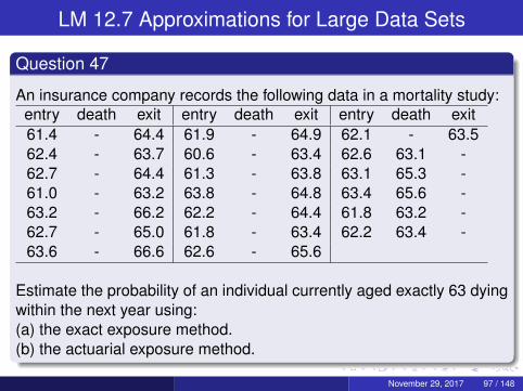
Question 47
An insurance company records the following data in a mortality study:entry death exit entry death exit entry death exit61.4 - 64.4 61.9 - 64.9 62.1 - 63.562.4 - 63.7 60.6 - 63.4 62.6 63.1 -62.7 - 64.4 61.3 - 63.8 63.1 65.3 -61.0 - 63.2 63.8 - 64.8 63.4 65.6 -63.2 - 66.2 62.2 - 64.4 61.8 63.2 -62.7 - 65.0 61.8 - 63.4 62.2 63.4 -63.6 - 66.6 62.6 - 65.6
Estimate the probability of an individual currently aged exactly 63 dyingwithin the next year using:(a) the exact exposure method.(b) the actuarial exposure method.
November 29, 2017 97 / 148
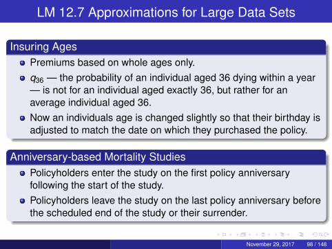
LM 12.7 Approximations for Large Data Sets
Insuring AgesPremiums based on whole ages only.q36 — the probability of an individual aged 36 dying within a year— is not for an individual aged exactly 36, but rather for anaverage individual aged 36.Now an individuals age is changed slightly so that their birthday isadjusted to match the date on which they purchased the policy.
Anniversary-based Mortality StudiesPolicyholders enter the study on the first policy anniversaryfollowing the start of the study.Policyholders leave the study on the last policy anniversary beforethe scheduled end of the study or their surrender.
November 29, 2017 98 / 148
LM 12.7 Approximations for Large Data Sets
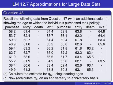
Question 48Recall the following data from Question 47 (with an additional columnshowing the age at which the individuals purchased their policy):purchase entry death exit purchase entry death exit
58.2 61.4 - 64.4 63.8 63.8 - 64.853.7 62.4 - 63.7 56.4 62.2 - 64.459.3 62.7 - 64.4 60.4 61.8 - 63.448.9 61.0 - 63.2 56.0 62.6 - 65.659.4 63.2 - 66.2 61.8 61.8 63.2 -62.7 62.7 - 65.0 62.2 62.2 63.4 -61.0 63.6 - 66.6 61.7 63.4 65.6 -55.2 61.9 - 64.9 55.0 62.1 - 63.538.4 60.6 - 63.4 52.4 62.6 63.1 -49.9 61.3 - 63.8 60.3 63.1 65.3 -
(a) Calculate the estimate for q63 using insuring ages.(b) Now recalculate q63 on an anniversary-to-anniversary basis.
November 29, 2017 99 / 148
LM 12.7 Approximations for Large Data Sets
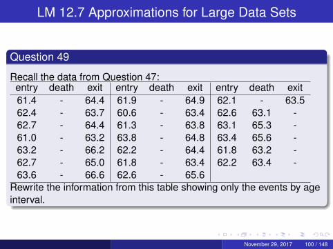
Question 49
Recall the data from Question 47:entry death exit entry death exit entry death exit61.4 - 64.4 61.9 - 64.9 62.1 - 63.562.4 - 63.7 60.6 - 63.4 62.6 63.1 -62.7 - 64.4 61.3 - 63.8 63.1 65.3 -61.0 - 63.2 63.8 - 64.8 63.4 65.6 -63.2 - 66.2 62.2 - 64.4 61.8 63.2 -62.7 - 65.0 61.8 - 63.4 62.2 63.4 -63.6 - 66.6 62.6 - 65.6
Rewrite the information from this table showing only the events by ageinterval.
November 29, 2017 100 / 148
LM 12.7 Approximations for Large Data Sets
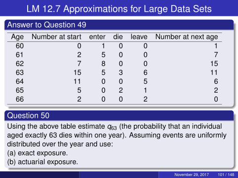
Answer to Question 49Age Number at start enter die leave Number at next age
60 0 1 0 0 161 2 5 0 0 762 7 8 0 0 1563 15 5 3 6 1164 11 0 0 5 665 5 0 2 1 266 2 0 0 2 0
Question 50Using the above table estimate q63 (the probability that an individualaged exactly 63 dies within one year). Assuming events are uniformlydistributed over the year and use:(a) exact exposure.(b) actuarial exposure.
November 29, 2017 101 / 148
LM 12.7 Approximations for Large Data Sets
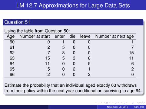
Question 51
Using the table from Question 50:Age Number at start enter die leave Number at next age
60 0 1 0 0 161 2 5 0 0 762 7 8 0 0 1563 15 5 3 6 1164 11 0 0 5 665 5 0 2 1 266 2 0 0 2 0
Estimate the probability that an individual aged exactly 63 withdrawsfrom their policy within the next year conditional on surviving to age 64.
November 29, 2017 102 / 148
LM 12.9 Estimation of Transition Intensities
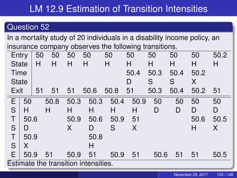
Question 52In a mortality study of 20 individuals in a disability income policy, aninsurance company observes the following transitions.Entry 50 50 50 50 50 50 50 50 50 50.2State H H H H H H H H H HTime 50.4 50.3 50.4 50.2State D S S XExit 51 51 51 50.6 50.8 51 50.3 50.4 50.2 51E 50 50.8 50.3 50.3 50.4 50.9 50 50 50 50S H H H H H H D D D DT 50.6 50.9 50.6 50.9 51 50.6 50.5S D X D S X H XT 50.9 50.8S X HE 50.9 51 50.9 51 50.9 51 50.6 51 51 50.5
Estimate the transition intensities.November 29, 2017 103 / 148

10.2 Introduction to Pensions
Reasons for Employers Offering PensionsCompetition for new employeesFacilitate retirement of older employees.Provide an incentive for employees to remain with theorganisation.Pressure from trade unions.Tax efficiencySocial Responsibility
November 29, 2017 104 / 148
Types of Pension Plan
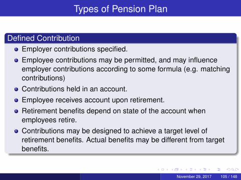
Defined ContributionEmployer contributions specified.Employee contributions may be permitted, and may influenceemployer contributions according to some formula (e.g. matchingcontributions)Contributions held in an account.Employee receives account upon retirement.Retirement benefits depend on state of the account whenemployees retire.Contributions may be designed to achieve a target level ofretirement benefits. Actual benefits may be different from targetbenefits.
November 29, 2017 105 / 148
Types of Pension Plan
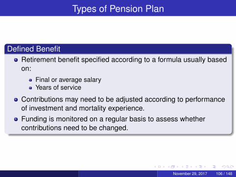
Defined BenefitRetirement benefit specified according to a formula usually basedon:
Final or average salaryYears of service
Contributions may need to be adjusted according to performanceof investment and mortality experience.Funding is monitored on a regular basis to assess whethercontributions need to be changed.
November 29, 2017 106 / 148
10.3 The Salary Scale Function
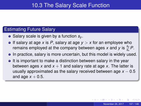
Estimating Future SalarySalary scale is given by a function sy .If salary at age x is P, salary at age y > x for an employee whoremains employed at the company between ages x and y is sy
sxP.
In practice, salary is more uncertain, but this model is widely used.It is important to make a distinction between salary in the yearbetween ages x and x + 1 and salary rate at age x . The latter isusually approximated as the salary received between age x − 0.5and age x + 0.5.
November 29, 2017 107 / 148
10.3 The Salary Scale Function
Question 53
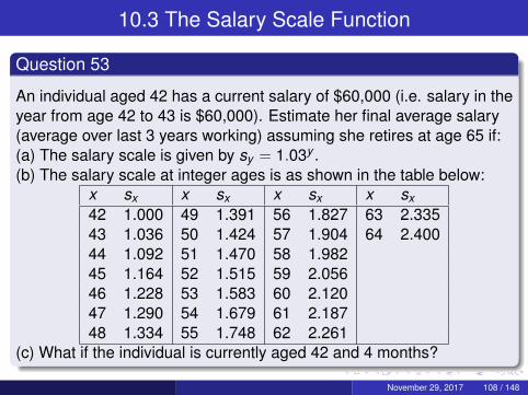
An individual aged 42 has a current salary of $60,000 (i.e. salary in theyear from age 42 to 43 is $60,000). Estimate her final average salary(average over last 3 years working) assuming she retires at age 65 if:(a) The salary scale is given by sy = 1.03y .(b) The salary scale at integer ages is as shown in the table below:
x sx x sx x sx x sx42 1.000 49 1.391 56 1.827 63 2.33543 1.036 50 1.424 57 1.904 64 2.40044 1.092 51 1.470 58 1.98245 1.164 52 1.515 59 2.05646 1.228 53 1.583 60 2.12047 1.290 54 1.679 61 2.18748 1.334 55 1.748 62 2.261
(c) What if the individual is currently aged 42 and 4 months?
November 29, 2017 108 / 148
10.4 Setting the DC Contribution
Question 54
An employer sets up a DC pension plan for its employees. The targetreplacement ratio is 60% of final average salary for an employee whoenters the plan at age exactly 30. Under the following assumptions:
At age 65, the employee will purchase a continuous life annuity,plus a continuous reversionary annuity valued at 50% of the lifeannuity.At age 65, the employee is married to someone aged 62.The salary scale is sy = 1.03y .Mortalities are independent and given by µx = 0.000002(1.093)x .A fixed percentage of salary is payable monthly in arrear.Contributions earn an annual rate of return of 6%.The value of a life annuity is based on a rate of interest of 4%.
Calculate the percentage of salary payable monthly.November 29, 2017 109 / 148
10.4 Setting the DC Contribution
Question 55
Recall from Question 54, that the rate of contribution was 20.74%.Calculate the actual replacement ratio achieved if the followingchanges are made to the assumptions:(a) At age 65, the employee is not married.(b) At age 65, the employee’s spouse is aged 73.(c) The rate of return on contributions is 7%.(d) Salary increases continuously at an annual rate of 5%.(e) At age 65, the employee purchases a whole life annuity, plus areversionary annuity for only 30% of the value.(f) The life annuities are valued using an interest rate of 3%.(g) The employee is in poor health at retirement, and has mortalitygiven by µx = 0.000002(1.143)x . [The employee’s spouse still hasmortality given by µx = 0.000002(1.093)x .]
November 29, 2017 110 / 148
10.5 The Service Table
Reasons for Early ExitWithdrawl — Leaving to take another job (or for other reasons).Early retirement.Disability retirement.Death.
November 29, 2017 111 / 148
10.5 The Service Table
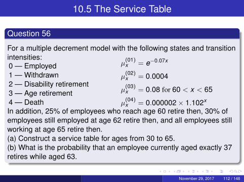
Question 56
For a multiple decrement model with the following states and transitionintensities:0 — Employed1 — Withdrawn2 — Disability retirement3 — Age retirement4 — Death
µ(01)x = e−0.07x
µ(02)x = 0.0004
µ(03)x = 0.08 for 60 < x < 65
µ(04)x = 0.000002× 1.102x
In addition, 25% of employees who reach age 60 retire then, 30% ofemployees still employed at age 62 retire then, and all employees stillworking at age 65 retire then.(a) Construct a service table for ages from 30 to 65.(b) What is the probability that an employee currently aged exactly 37retires while aged 63.
November 29, 2017 112 / 148
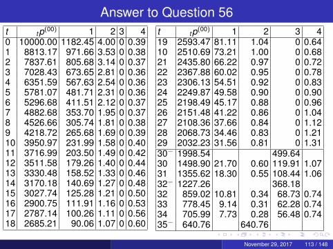
Answer to Question 56t tp(00) 1 2 3 40 10000.00 1182.45 4.00 0 0.391 8813.17 971.66 3.53 0 0.382 7837.61 805.68 3.14 0 0.373 7028.43 673.65 2.81 0 0.364 6351.59 567.63 2.54 0 0.365 5781.07 481.71 2.31 0 0.366 5296.68 411.51 2.12 0 0.377 4882.68 353.70 1.95 0 0.378 4526.66 305.74 1.81 0 0.389 4218.72 265.68 1.69 0 0.3910 3950.97 231.99 1.58 0 0.4011 3716.99 203.50 1.49 0 0.4212 3511.58 179.26 1.40 0 0.4413 3330.48 158.52 1.33 0 0.4614 3170.18 140.69 1.27 0 0.4815 3027.74 125.28 1.21 0 0.5016 2900.75 111.91 1.16 0 0.5317 2787.14 100.26 1.11 0 0.5618 2685.21 90.06 1.07 0 0.60
t tp(00) 1 2 3 419 2593.47 81.11 1.04 0 0.6410 2510.69 73.21 1.00 0 0.6821 2435.80 66.22 0.97 0 0.7222 2367.88 60.02 0.95 0 0.7823 2306.13 54.51 0.92 0 0.8324 2249.87 49.58 0.90 0 0.9025 2198.49 45.17 0.88 0 0.9626 2151.48 41.22 0.86 0 1.0427 2108.36 37.66 0.84 0 1.1228 2068.73 34.46 0.83 0 1.2129 2032.23 31.56 0.81 0 1.3130− 1998.54 499.6430 1498.90 21.70 0.60 119.91 1.0731 1355.62 18.30 0.55 108.44 1.0632− 1227.26 368.1832 859.02 10.81 0.34 68.73 0.7433 778.45 9.14 0.31 62.28 0.7434 705.99 7.73 0.28 56.48 0.7435− 640.76 640.76
November 29, 2017 113 / 148
10.6 Valuation of Benefits
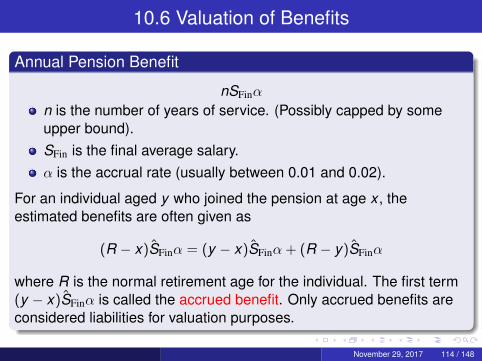
Annual Pension Benefit
nSFinα
n is the number of years of service. (Possibly capped by someupper bound).SFin is the final average salary.α is the accrual rate (usually between 0.01 and 0.02).
For an individual aged y who joined the pension at age x , theestimated benefits are often given as
(R − x)SFinα = (y − x)SFinα + (R − y)SFinα
where R is the normal retirement age for the individual. The first term(y − x)SFinα is called the accrued benefit. Only accrued benefits areconsidered liabilities for valuation purposes.
November 29, 2017 114 / 148
10.6 Valuation of Benefits
Projected vs. Current Unit MethodProjected Unit Method uses estimated future salary at retirement.Traditional or Current Unit Method uses current final averagesalary.
November 29, 2017 115 / 148
10.6 Valuation of Benefits
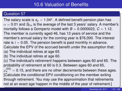
Question 57The salary scale is sy = 1.04y . A defined benefit pension plan hasα = 0.01 and SFin is the average of the last 3 years’ salary. A member’smortality follows a Gompertz model with B = 0.0000023, C = 1.12.The member is currently aged 46, has 13 years of service and themember’s annual salary for the coming year is $76,000. The interestrate is i = 0.05. The pension benefit is paid monthly in advance.Calculate the EPV of the accrued benefit under the assumption that:(a) The individual retires at age 65.(b) The individual retires at age 60.(c) The individual’s retirement happens between ages 60 and 65. Theprobability of retirement at 60 is 0.3. Between ages 60 and 65,µ
(03)x = 0.15, and there are no other decrements between these ages.
[Calculate the conditional EPV conditioning on the member exitingthrough retirement. You may use the approximation that retirementsnot at an exact age happen in the middle of the year of retirement.]
November 29, 2017 116 / 148
10.6 Valuation of Benefits
Question 58
An employee aged 43 has been working for a company for 15 years.The salary scale is sy = 1.05y . The employee’s salary last year was$75,000. If the employee withdraws from the pension plan, he receivesa deferred pension based on accrual rate 2%, with COLA of 2% peryear. He receives the pension starting from age 65 with paymentsmonthly in advance. The individual’s mortality is given byµ
(04)x = 0.000002× 1.102x . The interest rate is i = 0.04.
(a) Calculate the EPV of the pension benefits if he withdraws now.(b) Calculate the EPV of the accrued withdrawl benefits if the rate ofwithdrawl is µ(01)
x = e−0.07x .
November 29, 2017 117 / 148
10.6 Valuation of Benefits
Question 59
Let the salary scale be sy = 1.04y . A pension plan has benefit definedby α = 0.015 and SFin is the average of the last 3 years’ salary.Suppose a member’s mortality follows a Gompertz model withB = 0.0000023, C = 1.12. The member is currently aged 46 and has13 years of service, and a current annual salary of $45,000. The rateof withdrawl from the pension plan is µ(01)
x = e−0.07x . The individual willretire at age 60 with probability 0.3; will retire at rate µ(03)
x = 0.06between ages 60 and 65; and will retire at age 65 if still employed atthat age. The interest rate is i = 0.06 while the employee is employed.Once the employee exits the plan, the benefits are calculated at aninterest rate i = 0.05. The pension benefit is paid monthly in advance.Upon withdrawl, the employee receives a deferred pension with COLA2%. There is no death benefit. Calculate the EPV of the accruedbenefit of the employee.
November 29, 2017 118 / 148
10.6 Valuation of Benefits
Question 60
A pension plan offers a benefit of 4% of career average earnings peryear of service. The benefit is payable monthly in advance. Mortalityfollows a Gompertz model with B = 0.0000023, C = 1.12. The salaryscale is sy = 1.04y . One plan member aged 44 joined the plan 6 yearsago with a starting salary rate of $180,000. Withdrawls receive adeferred pension benefit from age 65, with COLA of 2%. The rate ofwithdrawl from the pension plan is µ(01)
x = e−0.07x . The individual willretire at age 60 with probability 0.3; will retire at rate µ(03)
x = 0.06between ages 60 and 65; and will retire at age 65 if still employed atthat age. The interest rate is i = 0.06 while the employee is employed.Once the employee exits the plan, the benefits are calculated at aninterest rate i = 0.05. There is no death benefit. Calculate the EPV ofthe accrued benefit.
November 29, 2017 119 / 148
10.7 Funding the Benefits
Funding DB Pension PlansEmployee pays fixed contribution (as percentage of salary).Employer pays the remaining costs of benefits.Employer contributions not usually specified in contract. Employerhas an incentive to keep its contributions smooth and predictable.Employer will usually establish a reserve level equal to the EPV ofaccrued liabilities, called Actuarial Liability.
Normal contribution Ct at start of year satisfies
tV + Ct = EPV of benefits for exits during the year + (1 + i)−11p00
x t+1V
November 29, 2017 120 / 148
10.7 Funding the Benefits
Question 61
An individual aged 45 has 26 years of service, and a last year’s salaryof $47,000. The salary scale is sy = 1.05y , and the accrual rate is0.02. The interest rate is i = 0.04. There is no death benefit. There areno exits other than death or retirement at age 65. Mortality follows aGompertz model with B = 0.0000076, C = 1.087. Calculate this year’semployer contribution to the plan using:(a) The Projected Unit Method.(b) The Traditional Unit Method.
November 29, 2017 121 / 148
10.7 Funding the Benefits
Question 62
Annual Pension benefits are 1% of final average salary over 3 yearsper year of service. The salary scale is sy = 1.06y . Mortality follows aGompertz model with B = 0.00000187, C = 1.130. The rate ofwithdrawl is µ01
x = 0.2e−0.04x . Withdrawl benefits take the form of adeferred pension with COLA 2%, beginning at age 65. The benefit fordeath while in service is 3 times the last year’s annual salary. Pensionbenefits are guaranteed for 5 years. Interest rates are 5%. Membersalive at age 60 retire then with probability 0.08. Members agedbetween 60 and 65 retire at a rate µ03
x = 0.1. Members who are stillemployed at age 65 all retire then. If a member aged 46 has 12 yearsof service and last year’s salary $87,000, and makes an annualcontribution of 4% of annual salary, calculate the employer’s annualcontribution to the pension plan on behalf of this member.
November 29, 2017 122 / 148
SN 5 Retiree Health BenefitsDifferences Between Retiree Health and Pension Benefits
Retiree Health Benefits are typically only offered to individualswho retire from the company.Usually Minimal Service RequirementsUsually not legally binding.Sometimes prefunded, sometimes paid from current income.Health benefits are not a linear function of years of service.Benefits do not depend on Salary.
Remarks on Retiree Health BenefitsUsually tops up government health-care provision.Usually claims are dealt with by a health insurance company.Costs to employers are the premiums.Premiums increase with age, and over time, usually aboveinflation.
November 29, 2017 123 / 148
SN 5 Retiree Health Benefits
Valuing Retirement Health BenefitsBenefits are a whole-life annuity with annual payments B(x , t) thepremium for an individual aged x in year t .We will assume interest rate is i , premiums are subject to inflationj and premiums increase by a factor c with age.We letaB(xr , t) = 1 + pxr (1 + j)c(1 + i)−1 + 2pxr (1 + j)2c2(1 + i)−2 + · · ·If we define 1 + i∗ = 1+i
c(1+j) , then aB(xr , t) = axr |i∗
If costs increase above the interest rate, i∗ will be negative.For an individual retiring at age xr at time t , the EPV of thebenefits is B(xr , t)axr |i∗ .We can use a linear method to calculate accrued benefit.We calculate the total accrued benefit by taking the expectationover time of retirement (using the service table).
November 29, 2017 124 / 148
SN 5 Retiree Health Benefits
Question 63
Why do we calculate the accrued benefits for each retirement age,rather than calculate total benefits first then calculate accrued value?
November 29, 2017 125 / 148
SN 5 Retiree Health Benefits
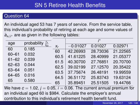
Question 64
An individual aged 53 has 7 years of service. From the service table,this individual’s probability of retiring at each age and some values ofaxr |i∗ are as given in the following tables:
age probability rxl53
60 0.18560–61 0.03261–62 0.03962–63 0.04463–64 0.05164–65 0.01665 0.580
i∗
xr −0.01027 0.01027 0.0297160 42.26993 28.73036 21.2256560.5 41.61225 28.40999 21.0537761.5 40.30700 27.76851 20.7070062.5 39.02199 27.12570 20.3542263.5 37.75674 26.48191 19.9955964.5 36.51172 25.83743 19.6312465 35.89451 25.51505 19.44766
We have c = 1.02, j = 0.05, i = 0.06. The current annual premium foran individual aged 60 is $984. Calculate the employer’s annualcontribution to this individual’s retirement health benefit fund.
November 29, 2017 126 / 148
12.3 Profit Testing a Term Insurance Policy
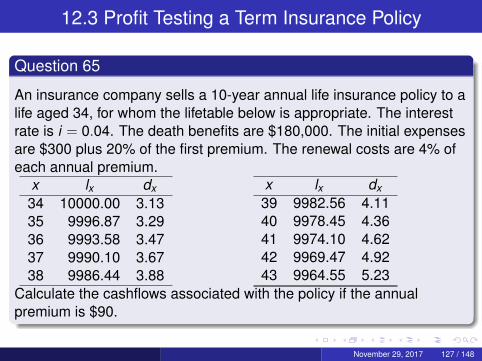
Question 65
An insurance company sells a 10-year annual life insurance policy to alife aged 34, for whom the lifetable below is appropriate. The interestrate is i = 0.04. The death benefits are $180,000. The initial expensesare $300 plus 20% of the first premium. The renewal costs are 4% ofeach annual premium.
x lx dx34 10000.00 3.1335 9996.87 3.2936 9993.58 3.4737 9990.10 3.6738 9986.44 3.88
x lx dx39 9982.56 4.1140 9978.45 4.3641 9974.10 4.6242 9969.47 4.9243 9964.55 5.23
Calculate the cashflows associated with the policy if the annualpremium is $90.
November 29, 2017 127 / 148
12.3 Profit Testing a Term Insurance Policy
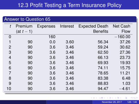
Answer to Question 65t Premium Expenses Interest Expected Death Net Cash
(at t − 1) Benefits Flow0 160 −160.001 90 0.0 3.60 56.34 37.262 90 3.6 3.46 59.24 30.623 90 3.6 3.46 62.50 27.364 90 3.6 3.46 66.13 23.735 90 3.6 3.46 69.93 19.936 90 3.6 3.46 74.11 15.757 90 3.6 3.46 78.65 11.218 90 3.6 3.46 83.38 6.489 90 3.6 3.46 88.83 1.03
10 90 3.6 3.46 94.47 −4.61
November 29, 2017 128 / 148
12.3 Profit Testing a Term Insurance Policy
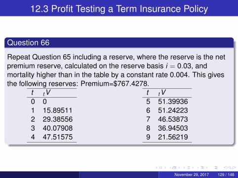
Question 66
Repeat Question 65 including a reserve, where the reserve is the netpremium reserve, calculated on the reserve basis i = 0.03, andmortality higher than in the table by a constant rate 0.004. This givesthe following reserves: Premium=$767.4278.
t tV0 01 15.895112 29.385563 40.079084 47.51575
t tV5 51.399366 51.242237 46.538738 36.945039 21.56219
November 29, 2017 129 / 148
12.3 Profit Testing a Term Insurance Policy
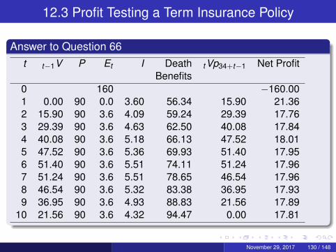
Answer to Question 66t t−1V P Et I Death tVp34+t−1 Net Profit
Benefits0 160 −160.001 0.00 90 0.0 3.60 56.34 15.90 21.362 15.90 90 3.6 4.09 59.24 29.39 17.763 29.39 90 3.6 4.63 62.50 40.08 17.844 40.08 90 3.6 5.18 66.13 47.52 18.015 47.52 90 3.6 5.36 69.93 51.40 17.956 51.40 90 3.6 5.51 74.11 51.24 17.967 51.24 90 3.6 5.51 78.65 46.54 17.968 46.54 90 3.6 5.32 83.38 36.95 17.939 36.95 90 3.6 4.93 88.83 21.56 17.89
10 21.56 90 3.6 4.32 94.47 0.00 17.81
November 29, 2017 130 / 148
12.3 Profit Testing a Term Insurance Policy
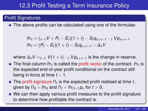
Profit SignaturesThe above profits can be calculated using one of the formulae:
Prt = (t−1V + Pt − Et )(1 + i)− Stqx+t−1 −t Vpx+t−1
Prt = (Pt − Et )(1 + i)− Stqx+t−1 −∆tV
where ∆tV =t−1 V (1 + i)−t Vpx+t−1 is the change in reserve.The final column Prt is called the profit vector of the contract. Prt isthe expected end-of-year profit conditional on the contract stillbeing in force at time t − 1.The profit signature Πt is the expected profit realised at time t ,given by Π0 = Pr0 and Πt = Prt t−1px for t > 0.We can then apply various profit measures to the profit signatureto determine how profitable the contract is.
November 29, 2017 131 / 148
12.3 Profit Testing a Term Insurance Policy
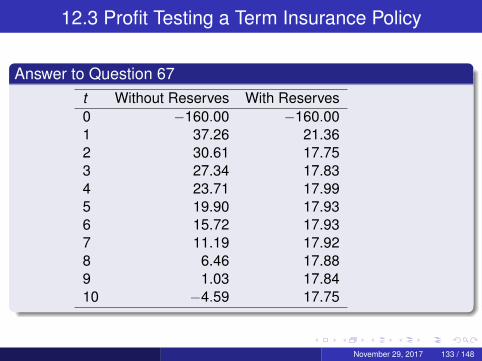
Question 67
Calculate the profit signatures for the contract in Question 65, both forthe original case and the case (Question 66) with reserves.
November 29, 2017 132 / 148
12.3 Profit Testing a Term Insurance Policy
Answer to Question 67t Without Reserves With Reserves0 −160.00 −160.001 37.26 21.362 30.61 17.753 27.34 17.834 23.71 17.995 19.90 17.936 15.72 17.937 11.19 17.928 6.46 17.889 1.03 17.8410 −4.59 17.75
November 29, 2017 133 / 148

12.4 Profit Testing Principles
Notes on Profit TestingEasy to adapt this to Multiple Decrement Models.Profit testing is usually applied to a portfolio of policies, rather thana single policy.We have replaced random variables by their expected values.This is called deterministic profit testing.The profit signature is used to assess profitability. The profit vectoris used for policies already in force.We will cover stochastic profit testing and profit testing formultiple-state models later.
November 29, 2017 134 / 148
12.5 Profit Measures
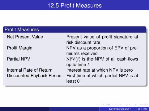
Profit MeasuresNet Present Value Present value of profit signature at
risk discount rateProfit Margin NPV as a proportion of EPV of pre-
miums receivedPartial NPV NPV(t) is the NPV of all cash-flows
up to time tInternal Rate of Return Interest rate at which NPV is zeroDiscounted Payback Period First time at which partial NPV is at
least 0
November 29, 2017 135 / 148
12.5 Profit Measures
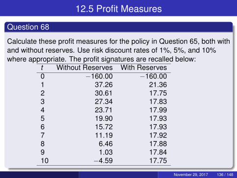
Question 68
Calculate these profit measures for the policy in Question 65, both withand without reserves. Use risk discount rates of 1%, 5%, and 10%where appropriate. The profit signatures are recalled below:
t Without Reserves With Reserves0 −160.00 −160.001 37.26 21.362 30.61 17.753 27.34 17.834 23.71 17.995 19.90 17.936 15.72 17.937 11.19 17.928 6.46 17.889 1.03 17.8410 −4.59 17.75
November 29, 2017 136 / 148
12.5 Profit Measures
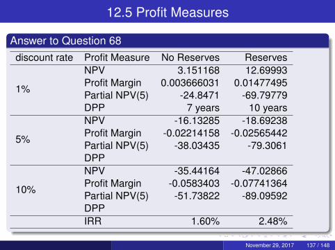
Answer to Question 68discount rate Profit Measure No Reserves Reserves
1%
NPV 3.151168 12.69993Profit Margin 0.003666031 0.01477495Partial NPV(5) -24.8471 -69.79779DPP 7 years 10 years
5%
NPV -16.13285 -18.69238Profit Margin -0.02214158 -0.02565442Partial NPV(5) -38.03435 -79.3061DPP
10%
NPV -35.44164 -47.02866Profit Margin -0.0583403 -0.07741364Partial NPV(5) -51.73822 -89.09592DPPIRR 1.60% 2.48%
November 29, 2017 137 / 148

12.6 Using the Profit Test to Calculate the Premium
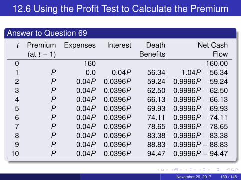
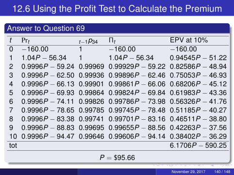
Question 69
For the policy in Question 65, calculate the premium that achieves arisk discount rate of 10%.
November 29, 2017 138 / 148
12.6 Using the Profit Test to Calculate the Premium
Answer to Question 69t Premium Expenses Interest Death Net Cash
(at t − 1) Benefits Flow0 160 −160.001 P 0.0 0.04P 56.34 1.04P − 56.342 P 0.04P 0.0396P 59.24 0.9996P − 59.243 P 0.04P 0.0396P 62.50 0.9996P − 62.504 P 0.04P 0.0396P 66.13 0.9996P − 66.135 P 0.04P 0.0396P 69.93 0.9996P − 69.936 P 0.04P 0.0396P 74.11 0.9996P − 74.117 P 0.04P 0.0396P 78.65 0.9996P − 78.658 P 0.04P 0.0396P 83.38 0.9996P − 83.389 P 0.04P 0.0396P 88.83 0.9996P − 88.83
10 P 0.04P 0.0396P 94.47 0.9996P − 94.47
November 29, 2017 139 / 148
12.6 Using the Profit Test to Calculate the Premium
Answer to Question 69t Prt t−1p34 Πt EPV at 10%0 −160.00 1 −160.00 −160.001 1.04P − 56.34 1 1.04P − 56.34 0.94545P − 51.222 0.9996P − 59.24 0.99969 0.99929P − 59.22 0.82586P − 48.943 0.9996P − 62.50 0.99936 0.99896P − 62.46 0.75053P − 46.934 0.9996P − 66.13 0.99901 0.99861P − 66.06 0.68206P − 45.125 0.9996P − 69.93 0.99864 0.99824P − 69.84 0.61983P − 43.366 0.9996P − 74.11 0.99826 0.99786P − 73.98 0.56326P − 41.767 0.9996P − 78.65 0.99785 0.99745P − 78.48 0.51185P − 40.278 0.9996P − 83.38 0.99741 0.99701P − 83.16 0.46511P − 38.809 0.9996P − 88.83 0.99695 0.99655P − 88.56 0.42263P − 37.5610 0.9996P − 94.47 0.99646 0.99606P − 94.14 0.38402P − 36.29tot 6.1706P − 590.25
P = $95.66
November 29, 2017 140 / 148
12.7 Using the Profit Test to Calculate Reserves
Question 70
Calculate the reserves for the policy in Question 65 so that no year hasa negative cash flow.
November 29, 2017 141 / 148
12.7 Using the Profit Test to Calculate Reserves
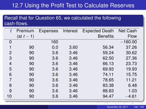
Recall that for Question 65, we calculated the followingcash-flows.
t Premium Expenses Interest Expected Death Net Cash(at t − 1) Benefits Flow
0 160 −160.001 90 0.0 3.60 56.34 37.262 90 3.6 3.46 59.24 30.623 90 3.6 3.46 62.50 27.364 90 3.6 3.46 66.13 23.735 90 3.6 3.46 69.93 19.936 90 3.6 3.46 74.11 15.757 90 3.6 3.46 78.65 11.218 90 3.6 3.46 83.38 6.489 90 3.6 3.46 88.83 1.03
10 90 3.6 3.46 94.47 −4.61
November 29, 2017 142 / 148
12.8 Profit Testing for Multiple-State Models
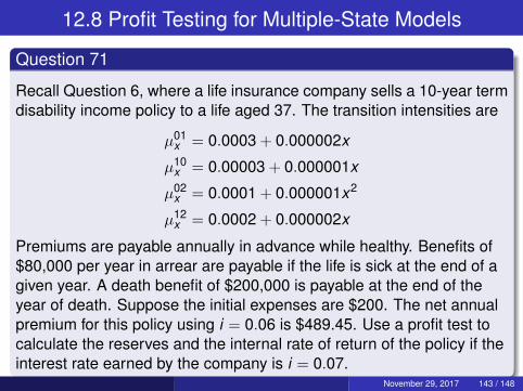
Question 71
Recall Question 6, where a life insurance company sells a 10-year termdisability income policy to a life aged 37. The transition intensities are
µ01x = 0.0003 + 0.000002x
µ10x = 0.00003 + 0.000001x
µ02x = 0.0001 + 0.000001x2
µ12x = 0.0002 + 0.000002x
Premiums are payable annually in advance while healthy. Benefits of$80,000 per year in arrear are payable if the life is sick at the end of agiven year. A death benefit of $200,000 is payable at the end of theyear of death. Suppose the initial expenses are $200. The net annualpremium for this policy using i = 0.06 is $489.45. Use a profit test tocalculate the reserves and the internal rate of return of the policy if theinterest rate earned by the company is i = 0.07.
November 29, 2017 143 / 148
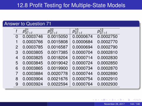
12.8 Profit Testing for Multiple-State Models
Answer to Question 71t p01
37+t p0237+t p10
37+t p1237+t
0 0.0003746 0.0015050 0.0000674 0.00027501 0.0003766 0.0015808 0.0000684 0.00027702 0.0003785 0.0016587 0.0000694 0.00027903 0.0003805 0.0017385 0.0000704 0.00028104 0.0003825 0.0018204 0.0000714 0.00028305 0.0003845 0.0019042 0.0000724 0.00028506 0.0003865 0.0019900 0.0000734 0.00028707 0.0003884 0.0020778 0.0000744 0.00028908 0.0003904 0.0021676 0.0000754 0.00029109 0.0003924 0.0022594 0.0000764 0.0002930
November 29, 2017 144 / 148
12.8 Profit Testing for Multiple-State Models
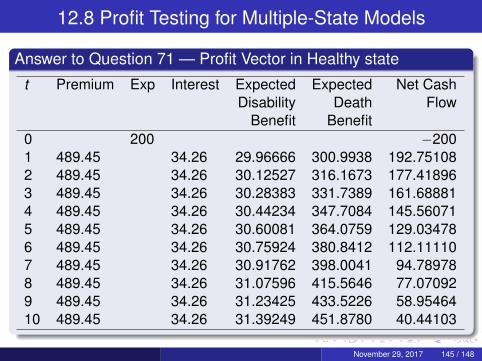
Answer to Question 71 — Profit Vector in Healthy state
t Premium Exp Interest Expected Expected Net CashDisability Death Flow
Benefit Benefit0 200 −2001 489.45 34.26 29.96666 300.9938 192.751082 489.45 34.26 30.12527 316.1673 177.418963 489.45 34.26 30.28383 331.7389 161.688814 489.45 34.26 30.44234 347.7084 145.560715 489.45 34.26 30.60081 364.0759 129.034786 489.45 34.26 30.75924 380.8412 112.111107 489.45 34.26 30.91762 398.0041 94.789788 489.45 34.26 31.07596 415.5646 77.070929 489.45 34.26 31.23425 433.5226 58.9546410 489.45 34.26 31.39249 451.8780 40.44103
November 29, 2017 145 / 148
12.8 Profit Testing for Multiple-State Models
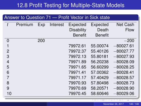
Answer to Question 71 — Profit Vector in Sick statet Premium Exp Interest Expected Expected Net Cash
Disability Death FlowBenefit Benefit
0 200 −2001 79972.61 55.00074 −80027.612 79972.37 55.40126 −80027.773 79972.13 55.80181 −80027.934 79971.89 56.20238 −80028.095 79971.65 56.60299 −80028.256 79971.41 57.00362 −80028.417 79971.17 57.40429 −80028.578 79970.93 57.80498 −80028.739 79970.69 58.20571 −80028.9010 79970.45 58.60646 −80029.06
November 29, 2017 146 / 148
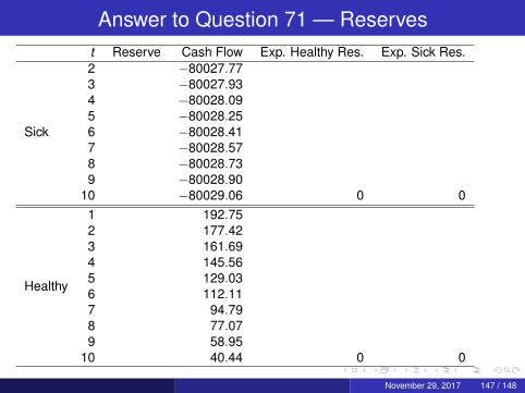
Answer to Question 71 — Reservest Reserve Cash Flow Exp. Healthy Res. Exp. Sick Res.
Sick
2 −80027.773 −80027.934 −80028.095 −80028.256 −80028.417 −80028.578 −80028.739 −80028.90
10 −80029.06 0 0
Healthy
1 192.752 177.423 161.694 145.565 129.036 112.117 94.798 77.079 58.95
10 40.44 0 0
November 29, 2017 147 / 148
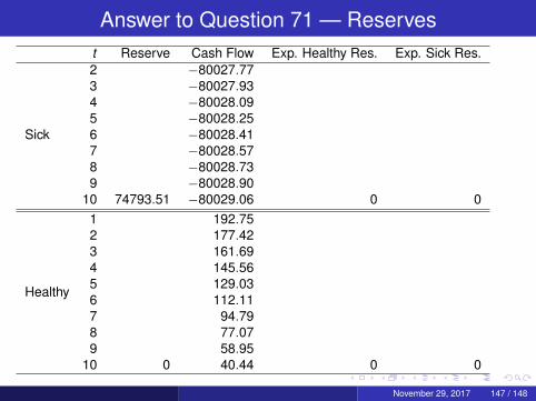
Answer to Question 71 — Reservest Reserve Cash Flow Exp. Healthy Res. Exp. Sick Res.
Sick
2 −80027.773 −80027.934 −80028.095 −80028.256 −80028.417 −80028.578 −80028.739 −80028.90
10 74793.51 −80029.06 0 0
Healthy
1 192.752 177.423 161.694 145.565 129.036 112.117 94.798 77.079 58.95
10 0 40.44 0 0
November 29, 2017 147 / 148
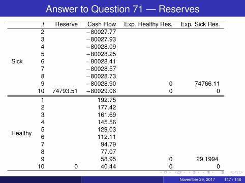
Answer to Question 71 — Reservest Reserve Cash Flow Exp. Healthy Res. Exp. Sick Res.
Sick
2 −80027.773 −80027.934 −80028.095 −80028.256 −80028.417 −80028.578 −80028.739 −80028.90 0 74766.11
10 74793.51 −80029.06 0 0
Healthy
1 192.752 177.423 161.694 145.565 129.036 112.117 94.798 77.079 58.95 0 29.1994
10 0 40.44 0 0
November 29, 2017 147 / 148
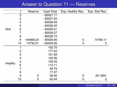
Answer to Question 71 — Reservest Reserve Cash Flow Exp. Healthy Res. Exp. Sick Res.
Sick
2 −80027.773 −80027.934 −80028.095 −80028.256 −80028.417 −80028.578 −80028.739 144668.23 −80028.90 0 74766.11
10 74793.51 −80029.06 0 0
Healthy
1 192.752 177.423 161.694 145.565 129.036 112.117 94.798 77.079 0 58.95 0 29.1994
10 0 40.44 0 0
November 29, 2017 147 / 148
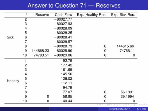
Answer to Question 71 — Reservest Reserve Cash Flow Exp. Healthy Res. Exp. Sick Res.
Sick
2 −80027.773 −80027.934 −80028.095 −80028.256 −80028.417 −80028.578 −80028.73 0 144615.669 144668.23 −80028.90 0 74766.11
10 74793.51 −80029.06 0 0
Healthy
1 192.752 177.423 161.694 145.565 129.036 112.117 94.798 77.07 0 56.18919 0 58.95 0 29.1994
10 0 40.44 0 0
November 29, 2017 147 / 148
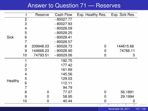
Answer to Question 71 — Reservest Reserve Cash Flow Exp. Healthy Res. Exp. Sick Res.
Sick
2 −80027.773 −80027.934 −80028.095 −80028.256 −80028.417 −80028.578 209948.03 −80028.73 0 144615.669 144668.23 −80028.90 0 74766.11
10 74793.51 −80029.06 0 0
Healthy
1 192.752 177.423 161.694 145.565 129.036 112.117 94.798 0 77.07 0 56.18919 0 58.95 0 29.1994
10 0 40.44 0 0
November 29, 2017 147 / 148
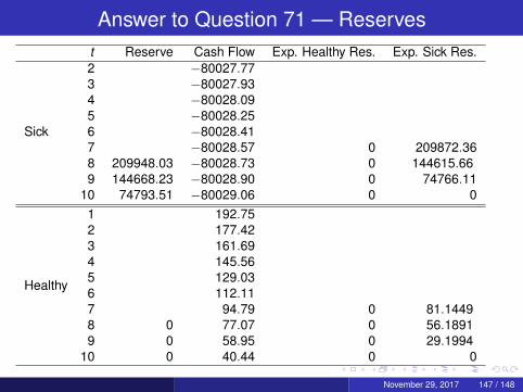
Answer to Question 71 — Reservest Reserve Cash Flow Exp. Healthy Res. Exp. Sick Res.
Sick
2 −80027.773 −80027.934 −80028.095 −80028.256 −80028.417 −80028.57 0 209872.368 209948.03 −80028.73 0 144615.669 144668.23 −80028.90 0 74766.11
10 74793.51 −80029.06 0 0
Healthy
1 192.752 177.423 161.694 145.565 129.036 112.117 94.79 0 81.14498 0 77.07 0 56.18919 0 58.95 0 29.1994
10 0 40.44 0 0
November 29, 2017 147 / 148

Answer to Question 71 — Reservest Reserve Cash Flow Exp. Healthy Res. Exp. Sick Res.
Sick
2 −80027.773 −80027.934 −80028.095 −80028.256 −80028.417 270935.45 −80028.57 0 209872.368 209948.03 −80028.73 0 144615.669 144668.23 −80028.90 0 74766.11
10 74793.51 −80029.06 0 0
Healthy
1 192.752 177.423 161.694 145.565 129.036 112.117 0 94.79 0 81.14498 0 77.07 0 56.18919 0 58.95 0 29.1994
10 0 40.44 0 0
November 29, 2017 147 / 148

Answer to Question 71 — Reservest Reserve Cash Flow Exp. Healthy Res. Exp. Sick Res.
Sick
2 −80027.773 −80027.934 −80028.095 −80028.256 −80028.41 0 270838.627 270935.45 −80028.57 0 209872.368 209948.03 −80028.73 0 144615.669 144668.23 −80028.90 0 74766.11
10 74793.51 −80029.06 0 0
Healthy
1 192.752 177.423 161.694 145.565 129.036 112.11 0 104.17477 0 94.79 0 81.14498 0 77.07 0 56.18919 0 58.95 0 29.1994
10 0 40.44 0 0
November 29, 2017 147 / 148
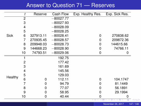
Answer to Question 71 — Reservest Reserve Cash Flow Exp. Healthy Res. Exp. Sick Res.
Sick
2 −80027.773 −80027.934 −80028.095 −80028.256 327913.11 −80028.41 0 270838.627 270935.45 −80028.57 0 209872.368 209948.03 −80028.73 0 144615.669 144668.23 −80028.90 0 74766.11
10 74793.51 −80029.06 0 0
Healthy
1 192.752 177.423 161.694 145.565 129.036 0 112.11 0 104.17477 0 94.79 0 81.14498 0 77.07 0 56.18919 0 58.95 0 29.1994
10 0 40.44 0 0
November 29, 2017 147 / 148

Answer to Question 71 — Reservest Reserve Cash Flow Exp. Healthy Res. Exp. Sick Res.
Sick
2 −80027.773 −80027.934 −80028.095 −80028.25 0 327796.906 327913.11 −80028.41 0 270838.627 270935.45 −80028.57 0 209872.368 209948.03 −80028.73 0 144615.669 144668.23 −80028.90 0 74766.11
10 74793.51 −80029.06 0 0
Healthy
1 192.752 177.423 161.694 145.565 129.03 0 125.42686 0 112.11 0 104.17477 0 94.79 0 81.14498 0 77.07 0 56.18919 0 58.95 0 29.1994
10 0 40.44 0 0
November 29, 2017 147 / 148
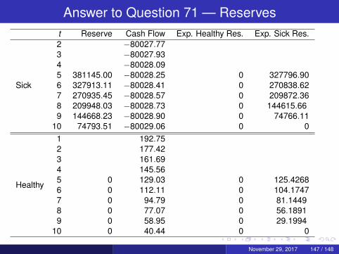
Answer to Question 71 — Reservest Reserve Cash Flow Exp. Healthy Res. Exp. Sick Res.
Sick
2 −80027.773 −80027.934 −80028.095 381145.00 −80028.25 0 327796.906 327913.11 −80028.41 0 270838.627 270935.45 −80028.57 0 209872.368 209948.03 −80028.73 0 144615.669 144668.23 −80028.90 0 74766.11
10 74793.51 −80029.06 0 0
Healthy
1 192.752 177.423 161.694 145.565 0 129.03 0 125.42686 0 112.11 0 104.17477 0 94.79 0 81.14498 0 77.07 0 56.18919 0 58.95 0 29.1994
10 0 40.44 0 0
November 29, 2017 147 / 148
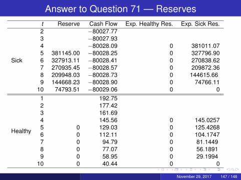
Answer to Question 71 — Reservest Reserve Cash Flow Exp. Healthy Res. Exp. Sick Res.
Sick
2 −80027.773 −80027.934 −80028.09 0 381011.075 381145.00 −80028.25 0 327796.906 327913.11 −80028.41 0 270838.627 270935.45 −80028.57 0 209872.368 209948.03 −80028.73 0 144615.669 144668.23 −80028.90 0 74766.11
10 74793.51 −80029.06 0 0
Healthy
1 192.752 177.423 161.694 145.56 0 145.02575 0 129.03 0 125.42686 0 112.11 0 104.17477 0 94.79 0 81.14498 0 77.07 0 56.18919 0 58.95 0 29.1994
10 0 40.44 0 0
November 29, 2017 147 / 148
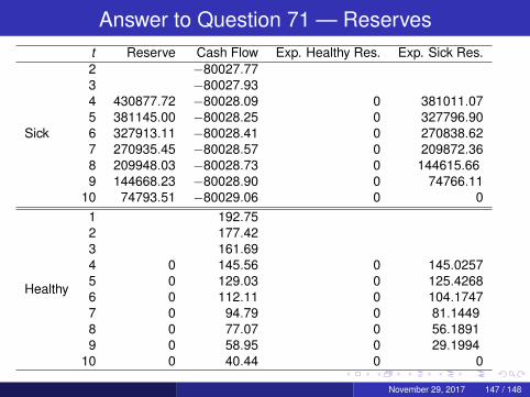
Answer to Question 71 — Reservest Reserve Cash Flow Exp. Healthy Res. Exp. Sick Res.
Sick
2 −80027.773 −80027.934 430877.72 −80028.09 0 381011.075 381145.00 −80028.25 0 327796.906 327913.11 −80028.41 0 270838.627 270935.45 −80028.57 0 209872.368 209948.03 −80028.73 0 144615.669 144668.23 −80028.90 0 74766.11
10 74793.51 −80029.06 0 0
Healthy
1 192.752 177.423 161.694 0 145.56 0 145.02575 0 129.03 0 125.42686 0 112.11 0 104.17477 0 94.79 0 81.14498 0 77.07 0 56.18919 0 58.95 0 29.1994
10 0 40.44 0 0
November 29, 2017 147 / 148
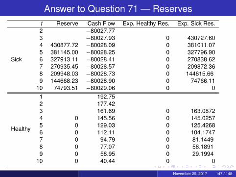
Answer to Question 71 — Reservest Reserve Cash Flow Exp. Healthy Res. Exp. Sick Res.
Sick
2 −80027.773 −80027.93 0 430727.604 430877.72 −80028.09 0 381011.075 381145.00 −80028.25 0 327796.906 327913.11 −80028.41 0 270838.627 270935.45 −80028.57 0 209872.368 209948.03 −80028.73 0 144615.669 144668.23 −80028.90 0 74766.11
10 74793.51 −80029.06 0 0
Healthy
1 192.752 177.423 161.69 0 163.08724 0 145.56 0 145.02575 0 129.03 0 125.42686 0 112.11 0 104.17477 0 94.79 0 81.14498 0 77.07 0 56.18919 0 58.95 0 29.1994
10 0 40.44 0 0
November 29, 2017 147 / 148
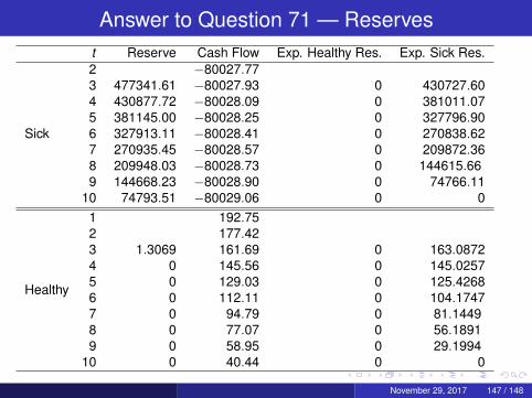
Answer to Question 71 — Reservest Reserve Cash Flow Exp. Healthy Res. Exp. Sick Res.
Sick
2 −80027.773 477341.61 −80027.93 0 430727.604 430877.72 −80028.09 0 381011.075 381145.00 −80028.25 0 327796.906 327913.11 −80028.41 0 270838.627 270935.45 −80028.57 0 209872.368 209948.03 −80028.73 0 144615.669 144668.23 −80028.90 0 74766.11
10 74793.51 −80029.06 0 0
Healthy
1 192.752 177.423 1.3069 161.69 0 163.08724 0 145.56 0 145.02575 0 129.03 0 125.42686 0 112.11 0 104.17477 0 94.79 0 81.14498 0 77.07 0 56.18919 0 58.95 0 29.1994
10 0 40.44 0 0
November 29, 2017 147 / 148
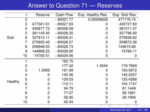
Answer to Question 71 — Reservest Reserve Cash Flow Exp. Healthy Res. Exp. Sick Res.
Sick
2 −80027.77 0.00008939 477176.743 477341.61 −80027.93 0 430727.604 430877.72 −80028.09 0 381011.075 381145.00 −80028.25 0 327796.906 327913.11 −80028.41 0 270838.627 270935.45 −80028.57 0 209872.368 209948.03 −80028.73 0 144615.669 144668.23 −80028.90 0 74766.11
10 74793.51 −80029.06 0 0
Healthy
1 192.752 177.42 1.3044 179.76693 1.3069 161.69 0 163.08724 0 145.56 0 145.02575 0 129.03 0 125.42686 0 112.11 0 104.17477 0 94.79 0 81.14498 0 77.07 0 56.18919 0 58.95 0 29.1994
10 0 40.44 0 0
November 29, 2017 147 / 148

Answer to Question 71 — Reservest Reserve Cash Flow Exp. Healthy Res. Exp. Sick Res.
Sick
2 520751.88 −80027.77 0.00008939 477176.743 477341.61 −80027.93 0 430727.604 430877.72 −80028.09 0 381011.075 381145.00 −80028.25 0 327796.906 327913.11 −80028.41 0 270838.627 270935.45 −80028.57 0 209872.368 209948.03 −80028.73 0 144615.669 144668.23 −80028.90 0 74766.11
10 74793.51 −80029.06 0 0
Healthy
1 192.752 3.4133 177.42 1.3044 179.76693 1.3069 161.69 0 163.08724 0 145.56 0 145.02575 0 129.03 0 125.42686 0 112.11 0 104.17477 0 94.79 0 81.14498 0 77.07 0 56.18919 0 58.95 0 29.1994
10 0 40.44 0 0
November 29, 2017 147 / 148

Answer to Question 71 — Reservest Reserve Cash Flow Exp. Healthy Res. Exp. Sick Res.
Sick
2 520751.88 −80027.77 0.00008939 477176.743 477341.61 −80027.93 0 430727.604 430877.72 −80028.09 0 381011.075 381145.00 −80028.25 0 327796.906 327913.11 −80028.41 0 270838.627 270935.45 −80028.57 0 209872.368 209948.03 −80028.73 0 144615.669 144668.23 −80028.90 0 74766.11
10 74793.51 −80029.06 0 0
Healthy
1 192.75 3.4069 195.07372 3.4133 177.42 1.3044 179.76693 1.3069 161.69 0 163.08724 0 145.56 0 145.02575 0 129.03 0 125.42686 0 112.11 0 104.17477 0 94.79 0 81.14498 0 77.07 0 56.18919 0 58.95 0 29.1994
10 0 40.44 0 0
November 29, 2017 147 / 148
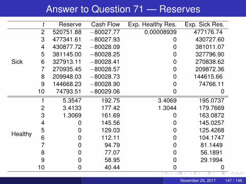
Answer to Question 71 — Reservest Reserve Cash Flow Exp. Healthy Res. Exp. Sick Res.
Sick
2 520751.88 −80027.77 0.00008939 477176.743 477341.61 −80027.93 0 430727.604 430877.72 −80028.09 0 381011.075 381145.00 −80028.25 0 327796.906 327913.11 −80028.41 0 270838.627 270935.45 −80028.57 0 209872.368 209948.03 −80028.73 0 144615.669 144668.23 −80028.90 0 74766.11
10 74793.51 −80029.06 0 0
Healthy
1 5.3547 192.75 3.4069 195.07372 3.4133 177.42 1.3044 179.76693 1.3069 161.69 0 163.08724 0 145.56 0 145.02575 0 129.03 0 125.42686 0 112.11 0 104.17477 0 94.79 0 81.14498 0 77.07 0 56.18919 0 58.95 0 29.1994
10 0 40.44 0 0
November 29, 2017 147 / 148
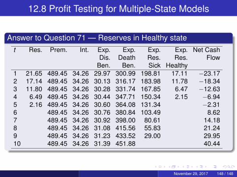
12.8 Profit Testing for Multiple-State Models
Answer to Question 71 — Reserves in Healthy statet Res. Prem. Int. Exp. Exp. Exp. Exp. Net Cash
Dis. Death Res. Res. FlowBen. Ben. Sick Healthy
1 21.65 489.45 34.26 29.97 300.99 198.81 17.11 −23.172 17.14 489.45 34.26 30.13 316.17 183.98 11.78 −18.343 11.80 489.45 34.26 30.28 331.74 167.85 6.47 −12.634 6.49 489.45 34.26 30.44 347.71 150.34 2.15 −6.945 2.16 489.45 34.26 30.60 364.08 131.34 −2.316 489.45 34.26 30.76 380.84 103.49 8.627 489.45 34.26 30.92 398.00 80.61 14.188 489.45 34.26 31.08 415.56 55.83 21.249 489.45 34.26 31.23 433.52 29.00 29.9510 489.45 34.26 31.39 451.88 40.44
November 29, 2017 148 / 148
Recommended


![Contingencies and provisioning[1]](https://img.pdfslide.us/doc/110x75/5457ed9faf795963388b5b66/contingencies-and-provisioning1.jpg)