Mathematical modelling of evapotranspiration byusing remote sensing and data miningLamya Neissi ( [email protected] )
Shahid Chamran University of AhvazMona Golabi
Shahid Chamran University of AhvazMohammad Albaji
Shahid Chamran University of AhvazAbd Ali Naseri
Shahid Chamran University of Ahvaz
Research Article
Keywords: Remote sensing, data mining, GIS, machine learning
Posted Date: April 5th, 2021
DOI: https://doi.org/10.21203/rs.3.rs-174771/v1
License: This work is licensed under a Creative Commons Attribution 4.0 International License. Read Full License

1
Mathematical modelling of evapotranspiration by using remote sensing and data mining 1
2
Lamya Neissi1, Mona Golabi2, Mohammad Albaji3, Abd Ali Naseri4 3
4
1Phd Student of Irrigation and Drainage, Department of Irrigation and Drainage, Faculty of 5
Water and Environmental Engineering, Shahid Chamran University of Ahvaz, Iran. E-mail: 6
8
2Assistance Professor, Department of Irrigation and Drainage, Faculty of Water and 9
Environmental Engineering, Shahid Chamran University of Ahvaz, Iran 10
Email: [email protected],[email protected] 11
12
*3 Assistance Professor, Department of Irrigation and Drainage, Faculty of Water and 13
Environmental Engineering, Shahid Chamran University of Ahvaz, Iran. 14
E-mail: [email protected]; [email protected] 15
16
17
4 Professor, Department of Irrigation and Drainage, Faculty of Water and Environmental 18
Engineering, Shahid Chamran University of Ahvaz, Iran. 19
E-mail: [email protected] 20
21
22
23
24

2
Abstract 25
Precise evaluation of evapotranspiration in an extended area is crucial for water requirement. By 26
using remote sensing evapotranspiration algorithms, many climatological variables are needed. 27
In case of using climatological variable measurements, many climatic stations must be 28
established in that specific area. By using data mining method integrated with remote sensing, 29
evapotranspiration can be calculated with high accuracy. A physical-based SEBAL 30
evapotranspiration algorithm was modeled by GIS model builder for ET calculations. Albedo, 31
emissivity, and Normalized Difference Water Index (NDWI) were considered as M5 decision 32
tree model inputs. Evapotranspiration was evaluated for 3 April 2020 to 17 September 2020 and 33
the equations were extracted in the M5 decision tree model and these equations were modeled in 34
GIS by using python scripts for 3 April 2020 to 17 September 2020. The results make clear that 35
the mathematical decision tree model can estimate the evapotranspiration gained by physical-36
based SEBAL algorithm in high accurately. 37
Keyword: Remote sensing; data mining; GIS; machine learning. 38
39
1. Introduction 40
Irrigation scheduling of crops can be done by using meteorological data for evapotranspiration 41
calculations. By using satellite images and different algorithms, evapotranspiration can be 42
estimated in an extended area and reach an accurate irrigation scheduling (Jaferian et al., 2019; 43
Song et al., 2018; Diarraa et al., 2017; Colaizzi et al., 2017; Anderson et al., 2012). 44
Evapotranspiration estimation is a complicated process. For estimating evapotranspiration, 45
different equations were obtained which can be used in different equations such as FAO-46
Penman–Monteith, Blaney-Criddle, etc. Ground observations represent the results for one 47
3
specific point in which high accuracy is needed to generalize them for extended region Hence 48
evaporation is different from station to station. By using remote sensing technologies, one can 49
reach acceptable and high accuracy for a specific extended region. By using satellite images as a 50
remote sensing technic, ground observations transformed to soft data. Among different methods 51
of data mining, the M5 decision tree was used to estimate the evapotranspiration in an extended 52
area (Gibert et al., 2018). 53
This research is intended to establish an applicable different linear relation by using the M5 54
decision tree between independent remote sensing parameters (albedo, emissivity, and 55
Normalized difference water index) with the dependent parameter (evapotranspiration) by using 56
data mining which is the most important innovation of this research. 57
Landsat8 satellite images and SEBAL algorithm were used for evapotranspiration estimation. 58
which was used in many evapotranspiration estimations and acceptable results obtained by these 59
researches (Mhawej et al., 2020; Elnmer et al., 2019; Kong et al., 2019; Ochege et al., 2019; 60
Gobbo et al., 2019; Kamali and Nazari, 2018). 61
Land surface temperature (LST) is one of input parameters for evapotranspiration estimation but 62
the spatial resolution of this band is 100m and the estimated evapotranspiration image by using 63
SEBAL algorithm by using this band has 100m spatial resolution. Which the other aim of this 64
research is to enhance spatial resolution by using the M5 decision tree. Input parameters have 65
30m spatial resolution and by applying the gained equations by the M5 decision tree, an 66
evapotranspiration map with higher spatial resolution can be obtained. 67
According to sugarcane plantation in an extended area in the southwest of Iran (more than 94000 68
ha), an extremely high volume of water is consumed in this section, so spatially enhancing 69

4
evapotranspiration estimation image, irrigation water scheduling can be calculated more 70
precisely. 71
72
2. Materials and methods 73
2.1. Study area 74
75
This study was conducted in the Amir-Kabir Agro-Industry Sugarcane fields. The Sugarcane 76
fields are located in the southwest of Iran (Figure1). The soil texture is clay-loam and annual 77
average evapotranspiration for 20 years was 3331.812 mm. The total area of cultivated sugarcane 78
in Khuzestan is over 84000 ha. Each farm has a low-pressure hydro flume irrigation system and 79
a subsurface drainage system with a 40m distance and 1.8 m depth for each drain tile. The total 80
irrigation water consumption is 3000 mm and the peak of irrigation water was applied in July. 81
82

5
83
Fig. 1. Amir-Kabir sugarcane Agro-Industry location area 84
85
2.2. Remote sensing 86
87
Landsat 8 OLI satellite images were the main data for remote sensing processes 88
(http://glovis.usgs.gov). Thermal bands have lower resolution compared to other optic bands. As 89
for Landsat8, band10 image represents a thermal band that provides less spatial resolution 90
(100m) but Thermal bands are critical for evapotranspiration estimation and Landsat8 has the 91
most appropriate thermal band for agricultural evapotranspiration estimation in a great variety 92

6
extended regions. Amir-Kabir agro-industry plantation with area of 14000 ha is extended enough 93
for evapotranspiration calculations by using remote sensing images. 94
95
2.3. Ground measurements 96
97
ET estimation requires meteorological data. Meteorological data were obtained from Amir-Kabir 98
agro-industry plantation local weather station. Weather data including Max and Min temperature, 99
the relative percentage of humidity, wind speed, and sunshine hours were used for 100
evapotranspiration calculations and Ref-et software was used for reference evapotranspiration 101
calculations. 102
103
2.4. SEBAL algorithm 104
105
The SEBAL algorithm was used to calculate the evapotranspiration (ET) of Sugarcane for the 106
Amir-Kabir agro-industry plantation. SEBAL algorithm uses thermal and multispectral digital 107
images of Landsat or other sensors to estimate the evapotranspiration (Bastiaanssen et al., 1998). 108
The ET calculation process is obtained by the amount of energy remained from the classical 109
equation of energy balance presented in equation (1): 110
λET = Rn − G – H (1)
111
7
Where λET is the latent heat flux in the atmospheric boundary layer (W/m2), Rn is the net 112
radiation (W/m2), H is the sensible heat flux (W/m2) and G is the soil heat flux (W/m2) (Allen et 113
al., 2002). 114
The net radiation (Rn) is computed by subtracting all outgoing radiant fluxes from all incoming 115
radiant fluxes. The soil heat flux (G) and sensible heat flux (H) are subtracted from the net 116
radiation flux at the surface Rn to compute the residual energy available for evapotranspiration 117
(λET) (Allen et al., 2002). The latent heat flux at the moment is converted into daily λET24 118
assuming a constant evaporative fraction (Ʌ) for 24 h calculated from the instantaneous energy 119
fluxes as observed in the satellite data as Eq. (2): 120
(2)
121
The daily actual evapotranspiration (ET24) can then be determined as Eq. (3): 122
(3)
Where Rn24 and G24 are the average net radiation for the day and daily soil heat flux (W/m2) 123
respectively which computed from raw products of instantaneous satellite spectral radiance, 124
vegetation indices, and satellite surface temperatures which are then expressed as average day 125
estimates (Singh et al., 2008). For this study, four cloud-free satellite images were obtained for 126

8
April 2019 and 2020. Actual evapotranspiration (ETa) maps in mm/day are generated by the 127
SEBAL algorithm for each day. 128
129
2.5. Data mining 130
Data science analysis Data Mining (DM) algorithms are the most fundamental components. 131
Certain DM techniques such as artificial neural networks, clustering, and case-based reasoning or 132
Bayesian networks have been applied in environmental modeling (Gibert et al., 2018). 133
Decision Tree methods uses the explanatory variables with higher discriminant power by 134
considering the response variable, then iteratively subdivide the training sample by building a 135
tree where the internal nodes are associated with the variables and its corresponding branches are 136
the possible values of the variable (Gibert et al., 2018). M5 Model Tree (introduced by Quinlan 137
in 1992), has linear regression functions at the leaf nodes, which develops a relationship between 138
input and output variables. Data are split into subsets and a decision tree is created. The data in 139
child nodes of splitting criterion depends on treating the standard deviation of the class values 140
and calculating the expected reduction in this error in consequence of testing each attribute at 141
that node. The standard deviation reduction (SDR) is calculated as Eq. (4) (Quinlan 1992): 142
143
(4)
144
Where T is a set of data that reaches the node, Ti is the subset of data that have the ith outcome 145
of the potential set and sd is the standard deviation (Rahimikhoob et al., 2013; Wang and Witten, 146

9
1997). the data in child nodes are purer due to a less standard deviation in comparison to parent 147
nodes. The M5 tree selects the one that maximizes the expected error reduction after scanning all 148
the possible splits. 149
150
If 151
152
153
154
155
156
157
158
159
160
161
Fig. 2. Structure of M5 decision tree (Models Y1–Y4 are linear regression models) 162
163
164
2.6. Model Inputs and Output 165
For estimating evapotranspiration by SEBAL algorithm, meteorological data are needed 166
including temperature, humidity, wind speed, etc. some inputs of SEBAL algorithm such as 167
albedo and emissivity are affected by the land surface temperature, so for using fewer variables 168
by data mining, albedo and emissivity were considered as inputs of M5 decision tree since these 169
two parameters are easy to get and better show the temperature variances. Also, transpiration 170
depends on the moisture of the plant. in data mining calculations, one vegetation index must 171
represent the plant moisture such as Normalized Difference Water Index (NDWI). So, albedo 172
and emissivity are represented as absorbed and transformed light to the atmosphere and NDWI is 173
1X
2X 2X
and and
≥ ? < ?
≥ ? ≥ ? < ? < ?
Then Then Then Then
1Y 2Y 3Y 4Y
Linear Model

10
represented as plant moisture. The main idea was to use the basic SEBAL equation (ET = Rn- G- 174
H) as a simple equation: ET = a(Albedo) – b(emissivity) – c(NDWI) and calculate the constant 175
values with M5 decision tree model. The three inputs of the M5 decision tree are explained 176
hereafter in more detail. 177
178
2.6.1. Evapotranspiration 179
One of the crucial parameters for evapotranspiration estimation is Land surface temperature 180
(LST) which Radiation and the exchange of energy flux between the earth's surface and 181
atmosphere depend on it (Weng et al., 2019). A physical model such as the SEBAL algorithm 182
has made it possible to estimate evapotranspiration for large areas. Surface biophysical 183
characteristics such as albedo, greenness, and wetness are among the most important parameters 184
affecting LST (Weng et al., 2019). The energy distribution is determined by albedo and 185
emissivity of the surface and atmosphere. previous studies show that surface emissivity strongly 186
correlates to vegetation cover (Griend and Owe, 1993; Rechid et al., 2009), vegetation also 187
strongly affects atmospheric properties through evapotranspiration (Gordon et al., 2005). 188
atmosphere emissivity is determined by atmospheric water vapor pressure (Staley and Jurica, 189
1972; Brutsaert, 1975). 190
191
2.6.2. Albedo 192
Albedo is a dimensionless diffuse reflectivity or reflecting power of a surface (Zhang et al., 193
2017) and is an important effective parameter on digital climate models and surface energy 194

11
balance equations (Zhang et al., 2017). Surface albedo is computed by correcting the αtoa for 195
atmospheric transmissivity as Eq. (5): 196
197
(5)
198
199
Where; α path_radiance is the average portion of the incoming solar radiation by considering all 200
bands that is back-scattered to the satellite before it reaches the earth’s surface, and τsw is the 201
atmospheric transmissivity (Allen et al., 2002). 202
203
2.6.3. Emissivity 204
205
The surface emissivity is the ratio of the actual radiation emitted by a surface to that emitted by a 206
black body at the same surface temperature (Allen et al., 2002). Surface emissivity is an 207
important variable for estimating land surface temperature and determining long-wave surface 208
energy balance (Mira et al., 2010). Sobrino et al. (2004) proposed emissivity based NDVI in 209
three different cases as Eq. (6): 210
211
(6)
212

12
Where εv is the vegetation canopy emissivity and εs is the bare soil emissivity; in this paper εv = 213
0.986 and εs = 0.973. the effect of the geometrical distribution of the natural surfaces is measured 214
as dε in Eq.6 . Pυ is the vegetation proportion obtained according to (Carlson and Ripley, 1997) 215
as Eq. (7): 216
217
(7)
218
The minimum value of the NDVI for bare soil over the study region is presented as NDVIS and 219
NDVIV is the highest NDVI for a fully vegetated pixel. The emissivity of land surfaces can differ 220
significantly by vegetation, surface moisture, and roughness (Nerry et al. 1988, Salisbury and 221
D’Aria 1992). 222
223
2.6.4. Vegetation Index 224
The NDWI spectral index which represents the crop moisture is the normalized difference water 225
index. NDWI has been used to estimate the equivalent water thickness of vegetation canopy 226
(Yilmaz et al., 2008). The NDWI considers two infrared bands with a central wavelength near 227
about 0.86 μm (NIR), and a central wavelength of about 1.24 μm (SWIR). The equation is 228
(Eq.8): 229
230
(8)
231

13
The M5 decision tree model takes Albedo, emissivity, and a vegetation index as input and after 232
the data mining process on these data, linear equations will be extracted. By inserting linear 233
equations, the evapotranspiration map was obtained as an output with higher spatial resolution. 234
Figure3 shows the flowchart of the M5 decision tree and SEBAL algorithm. 235
236
237
238
239
240
241
242
243
244
245
246
247
248
249
250

14
251
Fig. 3. Flowchart of the M5 decision tree and SEBAL algorithm 252
253
2.7. Model Validation 254
By using three inputs (albedo, emissivity, and NDWI) the accuracy of M5 decision tree was 255
evaluated. The accuracy of the M5 decision tree model and the final evapotranspiration map 256

15
which was combined with M5 decision tree was evaluated by correlation coefficient (R2), root 257
mean square errors (RMSE) and mean absolute errors (MAE) statistics (Eq. 9 to 11): 258
259
(9)
(10)
(11)
260
Where N is the number of data, ETo is the observed evaporation values calculated by the SEBAL 261
algorithm and ETp is the M5 decision tree model estimated evapotranspiration. 262
263
3. Results 264
265
3.1. M5 decision tree 266
For evapotranspiration estimation derivation M5 decision tree was used instead of SEBAL 267
physical-based model. By using decision tree for evapotranspiration estimation of two month, 268
different equations were extracted (Appendix1). The equations were obtained by using Albedo, 269
emissivity and Normalized difference vegetation index (NDWI) as model inputs. These three 270

16
input parameters were calculated from 6 June 2020 to 24 July 2020 and were considered as input 271
for each day of evapotranspiration estimation. 272
273
3.1.1. Inputs 274
3.1.1.1. Albedo 275
276
Albedo is the reflectance of solar energy from the earth’s surface. Albedo is said to determine 277
the amount of shortwave radiation to be absorbed by surfaces (Vargo et al., 2013). When 278
initial absorption of shortwave radiation is limited, it impacts the longwave energy radiated 279
by the earth’s surface, as well as energy availability for evapotranspiration and energy to be 280
converted to sensible heat. Ice, barren land, and sand have higher albedo, which causes 281
higher reflectance of shortwave radiation (Vargo et al., 2013). Vegetative land cover has a 282
lower albedo in comparison to barren land. 283
In this study albedo is one of model input parameters which was calculated for each image in 284
the study period. In the first growth stage of sugarcane, vegetative cover is very low and the 285
plant is not developed and canopy cover did not reach to its highest development. Figure 4 286
shows the albedo images as input parameters of the decision tree for the study duration. In 287
satellite images canopy cover area is much lower than soil area at the first growth stage 288
(figure 4, 3 April 2020, 12 May 2020). 289
290

17

18
291
Fig. 4. Albedo input images for M5 decision tree 292
293
At the end stage of sugarcane growth stage (24 July 2020, 17 September 2020) by developing 294
canopy cover of sugarcane most of the sun light absorbed by plant and less of the sun light 295
reflected to the atmosphere, therefore albedo amount is decreases. Calculated albedo images from 296
3 April till 17 September 2020 makes clear that by developing and growth of sugarcane plant 297
amount of albedo decreases and the canopy cover can affect the reflection of the sun light. 298
Calculated albedo images for input of M5 decision tree indicates that this parameter have an 299
acceptable spatial variability for evaluating evapotranspiration. 300
301
3.1.1.2. Emissivity 302
303
19
The emissivity of the surface of a material refers to the effectiveness of the surface in emitting 304
energy as thermal radiation (electromagnetic radiation with wavelength depending on the 305
temperature). Emissivity is mathematically defined as the ratio of the thermal radiation from the 306
surface to the radiation from an ideal black surface at the same temperature; the value varies 307
from 0 to 1. For C/SiC, the emissivity at 1600°C is ∼0.7, which is high (Alfano et al., 2009). 308
Emissivity as one input of the decision tree model related indirectly with Land Surface 309
Temperature (LST). Due to the increase of LST in the study period of sugarcane growth can 310
make the emissivity to increase. 311
Figure 5 shows the emissivity input parameter images for M5 decision tree model. Figure 5 312
indicates that at the first growth stage of sugarcane (figure5, 3 April 2020 and 12 May 2020) in 313
which the LST is low can make the emissivity to decrease considering less canopy cover and 314
more bare soil. 315
316
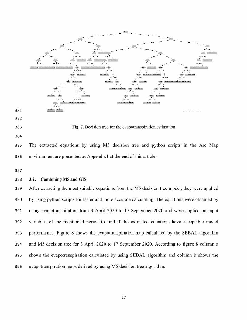
317

20

21
Fig. 5. Emissivity input images for M5 decision tree 318
319
In the end of sugarcane growth stage, the temperature increases which also makes the emissivity 320
to increase. Figure 5 makes clear that emissivity has suitable spatial variability which can make 321
the evaluation of evapotranspiration by using M5 decision tree with acceptable accuracy. 322
323
3.1.1.3. NDWI 324
325
The Normalized Difference Water Index (NDWI) (Gao, 1996) is a satellite-derived index from 326
the Near-Infrared (NIR) and Short Wave Infrared (SWIR) channels. The SWIR reflectance 327
reflects changes in both the vegetation water content and the spongy mesophyll structure in 328
vegetation canopies, while the NIR reflectance is affected by leaf internal structure and leaf dry 329
matter content but not by water content. The combination of the NIR with the SWIR removes 330
22
variations induced by leaf internal structure and leaf dry matter content, improving the accuracy 331
in retrieving the vegetation water content (Ceccato et al. 2001). The amount of water available in 332
the internal leaf structure largely controls the spectral reflectance in the SWIR interval of the 333
electromagnetic spectrum. SWIR reflectance is therefore negatively related to leaf water content 334
(Tucker, 1980). Its usefulness for drought monitoring and early warning has been demonstrated 335
in different studies (Gu et al., 2007; Ceccato et al., 2002). It is computed using the near infrared 336
(NIR) and the short wave infrared (SWIR) reflectance (Eq.8), which makes it sensitive to 337
changes in liquid water content and in spongy mesophyll of vegetation canopies (Gao, 1996 ; 338
Ceccato et al., 2001). 339
Figure 6 shows the NDWI input images for M5 decision tree. NDWI is considered as wetness 340
index of sugarcane. According to figure 6 NDWI varies in different growth stages and has wide 341
range of variability. In figure 6, 3 April 2020 and 12 May 2020 maximum and minimum amount 342
of NDWI differs spatially but due to early growth stage of the plant most of the cultivated area 343
are dry according to less irrigation water consumption. 344
Plant wetness status has effect on evapotranspiration, where plant with less wetness is under 345
water deficit stress and has less evapotranspiration and plant with high wetness index has high 346
evapotranspiration and this NDWI variability in different growth stages can obtain high accuracy 347
for evapotranspiration evaluation with data mining. 348
349
350
351
352

23

24

25
Fig. 6. NDWI input images for M5 decision tree 353
354
Also Figure 6 makes clear that in the end sugar cane growth stages most of the cultivated farms 355
have high NDWI index due to the peak of irrigation water requirement of sugarcane. 356
357
3.1.2. Output 358
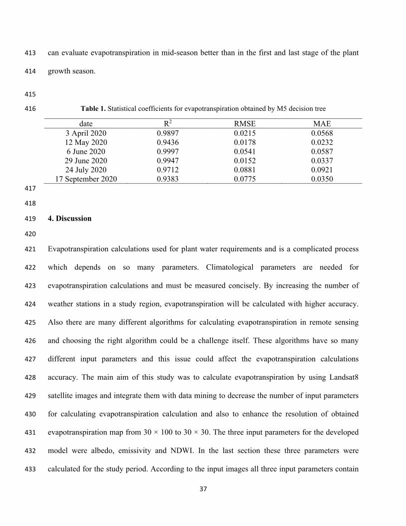
359
The values in parentheses under each label in the leaves indicate the number of segments 360
resulting from the corresponding threshold. The second value indicates the number of times a 361
misclassification occurred (Vieira et al., 2012) . 362

26
Figure 7 shows the decision tree for the evapotranspiration from 3 April 2020 to 17 September 363
2020. 45 different equations were extracted with a Correlation coefficient of 0.9947, Mean 364
absolute error and root mean squared error of 0.4101 and 0.5705, respectively . 365
By using fewer input parameters including albedo, emissivity, and NDWI, many 366
evapotranspiration equations were extracted. Figure 4 reveals that the albedo input variable was 367
located at the top of a decision tree which makes clear that albedo has high importance in 368
evapotranspiration estimation based on this decision tree. By considering the geographical 369
location of the study area, there is a high amount of receiving light in this area and the albedo 370
input variable was considered as absorbed light. Therefore, M5 decision tree divisions show that 371
the amount of absorbed light in this area has an important role in the evapotranspiration process 372
which most of the decision tree divisions were based on the albedo. NDWI variable is considered 373
as plant moisture which has an important role in evapotranspiration calculations after albedo 374
variable. This shows that the plant moisture has an important role in extracting the decision tree 375
equations beside the absorbed lights. 376
The emissivity variable was considered as the diffused light has less importance in the decision 377
tree divisions which by considering the geographical location of the study area it shows that most 378
of the received light was absorbed than diffused. 379
380
27
381
382
Fig. 7. Decision tree for the evapotranspiration estimation 383
384
The extracted equations by using M5 decision tree and python scripts in the Arc Map 385
environment are presented as Appendix1 at the end of this article. 386
387
3.2. Combining M5 and GIS 388
After extracting the most suitable equations from the M5 decision tree model, they were applied 389
by using python scripts for faster and more accurate calculating. The equations were obtained by 390
using evapotranspiration from 3 April 2020 to 17 September 2020 and were applied on input 391
variables of the mentioned period to find if the extracted equations have acceptable model 392
performance. Figure 8 shows the evapotranspiration map calculated by the SEBAL algorithm 393
and M5 decision tree for 3 April 2020 to 17 September 2020. According to figure 8 column a 394
shows the evapotranspiration calculated by using SEBAL algorithm and column b shows the 395
evapotranspiration maps derived by using M5 decision tree algorithm. 396

28
(a) (b)

29

30

31

32

33
397
Fig. 8. Evapotranspiration map calculated by SEBAL algorithm for column (a) and evapotranspiration 398
map calculated by M5 decision tree for column (b) 399
400
Figure 8 shows the results of the comparison between the SEBAL algorithm and M5 decision 401
tree for this two month study duration. Table 1 shows statistical coefficients for 3 April 2020 to 402
17 September 2020. According to figure 8 and table 1 by comparing the obtained results for 403
these two months, it could be possible to calculate evapotranspiration with fewer input. 404
Mathematical models can be used instead of physically-based models with acceptable accuracy. 405
406
407

34

35
R² = 0.9997
10
12
14
16
18
20
22
24
10 12 14 16 18 20 22 24
Evap
otr
an
pir
ati
on
d
eri
ved
by M
5
Evapotranpiration derived by SEBAL
6 June 2020

36
408
Fig. 9. Comparing the results between the SEBAL algorithm and M5 decision tree 409
410
According to Table 1, the calculated evapotranspiration for 6 and 29 June 2020 has obtained 411
better results than 17 September 2020. This is makes clear that the developed decision tree model 412
37
can evaluate evapotranspiration in mid-season better than in the first and last stage of the plant 413
growth season. 414
415
Table 1. Statistical coefficients for evapotranspiration obtained by M5 decision tree 416
date R2 RMSE MAE 3 April 2020 0.9897 0.0215 0.0568 12 May 2020 0.9436 0.0178 0.0232 6 June 2020 0.9997 0.0541 0.0587
29 June 2020 0.9947 0.0152 0.0337 24 July 2020 0.9712 0.0881 0.0921
17 September 2020 0.9383 0.0775 0.0350 417
418
4. Discussion 419
420
Evapotranspiration calculations used for plant water requirements and is a complicated process 421
which depends on so many parameters. Climatological parameters are needed for 422
evapotranspiration calculations and must be measured concisely. By increasing the number of 423
weather stations in a study region, evapotranspiration will be calculated with higher accuracy. 424
Also there are many different algorithms for calculating evapotranspiration in remote sensing 425
and choosing the right algorithm could be a challenge itself. These algorithms have so many 426
different input parameters and this issue could affect the evapotranspiration calculations 427
accuracy. The main aim of this study was to calculate evapotranspiration by using Landsat8 428
satellite images and integrate them with data mining to decrease the number of input parameters 429
for calculating evapotranspiration calculation and also to enhance the resolution of obtained 430
evapotranspiration map from 30 × 100 to 30 × 30. The three input parameters for the developed 431
model were albedo, emissivity and NDWI. In the last section these three parameters were 432
calculated for the study period. According to the input images all three input parameters contain 433

38
of acceptable variability and for better performance of data mining the input parameters should 434
have a suitable tolerance spatially and temporally. 435
The albedo input parameter or reflectivity represent the reflected light from the surface. The 436
reflected light from plant surface is much lesser than the soil surface. In the study region albedo 437
changes temporally and spatially in the cultivated area. In the first stage of plant growth most of 438
the light reflected to the atmosphere due to less developed canopy cover. By considering that the 439
plant need the light for photosynthesis and absorbs the light for this process, the absorbed light 440
effects on evapotranspiration and other life cycle processes of the plant. The albedo images 441
makes clear that during the growth season of the sugarcane the amount of absorbed light 442
increases, also the evapotranspiration increased in the study duration. This is indicate that the 443
absorbed light can effect on the evapotranspiration process. 444
Emissivity is the other input parameter of the decision tree model which related to LST and can 445
represent the temperature of the land surface cover because temperature of the environment can 446
effect on the plant evapotranspiration. Lansat8 satellite has a thermal band for calculating the 447
land surface temperature with resolution of 100m × 100m, so by using the calculated emissivity 448
instead of land surface temperature this resolution enhanced to 30m × 30m and without using the 449
thermal band and by using data mining decision tree method the resolution of evapotranspiration 450
map increases. 451
Wetness status of the plant and the environmental tensions can effect on evapotranspiration 452
process. NDWI can represent the water and wetness status of the sugarcane. This water index 453
differ spatially and temporally during the study season which can effect on the 454
evapotranspiration evaluation. 455

39
By using albedo as reflected light, emissivity representing the cover temperature and NDWI as 456
the water status of sugarcane, the evapotranspiration evaluated by using decision tree which in 457
the tree divisions started from the albedo input parameter and the albedo is the root of the 458
decision tree. By considering the location of the study area, the absorbed light has a significance 459
role in evapotranspiration evaluation. 460
Evapotranspiration calculated by using decision tree did not have a significance difference with 461
the evapotranspiration with calculated by using SEBAL algorithm. So by using data mining and 462
less input parameters evapotranspiration evaluated with acceptable accuracy and the resolution 463
of the evapotranspiration map enhanced to a higher resolution. 464
Also the main equation for calculating evapotranspiration in SEBAL algorithm is: λET = Rn – G 465
– H, which Rn is the net radiation (W/m2), G is the soil heat flux (W/m2) and H is the sensible 466
heat flux (W/m2). In this case albedo is considered as reflected light, emissivity is the land cover 467
temperature and NDWI is the water status of the land cover and the sugarcane. The main 468
equation obtained by the decision tree is: ET = (a×NDWI) – (b×Albedo) ± (c×emissivity). This 469
equation makes clear that evapotranspiration can be evaluated by using less input parameters and 470
indicate that water status of the plant can effect on evapotranspiration, when the water status is 471
suitable evapotranspiration increases and life mechanisms of the plant enhances. Also by 472
increasing the absorbed light, albedo decreases, hence the absorbed light has direct effect on the 473
plant evapotranspiration. The emissivity depends on land surface cover. Surfaces with soil cover 474
have lower emissivity comparing with plant cover surfaces. In plant cover surfaces with high 475
emissivity, evapotranspiration increases and soil surfaces with lower emissivity, 476
evapotranspiration decreases. So the main obtained equation conforms with the study region 477
40
conditions and it is suggested that apply this method to other case studies to find out if this 478
method could be used in a wide region. 479
480
5. Conclusion 481
482
This study discovered that by using less input parameters and selecting the right parameters, 483
evapotranspiration could be evaluated by using decision tree method and obtain acceptable 484
results. This is makes clear that indirect parameters related to evapotranspiration can be 485
considered as the main input parameters. The emissivity can represent the land canopy 486
temperature and due to low resolution of thermal band of Landsat satellite, the resolution of 487
evaluated evapotranspiration map enhanced to a higher resolution. Also the main equation for 488
calculating evapotranspiration in SEBAL algorithm is: λET = Rn – G – H, which Rn is the net 489
radiation (W/m2), G is the soil heat flux (W/m2) and H is the sensible heat flux (W/m2). In this 490
case albedo is considered as reflected light, emissivity is the land cover temperature and NDWI 491
is the water status of the land cover and the sugarcane. The obtained decision tree equations 492
(Appendix 1) show that the evapotranspiration could be calculated as: ET = (a×NDWI) – 493
(b×Albedo) ± (c×emissivity). This equation shows that evapotranspiration can be calculated by 494
using this three simple satellite parameters and by subtracting plant water status from reflected 495
light and addition or subtraction of emissivity (depend on land cover condition) with acceptable 496
accuracy. 497
6.Acknowledgments 498
We are grateful to the Research Council of Shahid Chamran University of Ahvaz for financial support 499
(GN:SCU.WI98.281). 500

41
Ethical Approval 501
Not applicable 502
Consent to participate 503
Consent was obtained from all individual participants included in the study. 504
Consent to publish 505
The participant has consented to the submission of the case report to the journal. 506
Author contribution 507
All authors contributed to the study conception and design. Material preparation, data collection and 508
analysis were performed by [Lamya Neissi], [Mona Golabi], [Mohammad Albaji] and [AbdAli Naseri]. 509
The first draft of the manuscript was written by [Lamya Neissi] and [Mohammad Albaji] and all authors 510
commented on previous versions of the manuscript. All authors read and approved the final manuscript. 511
Funding 512
This study was funded by “Shahid Chamran University of Ahvaz”. 513
Competing Interests 514
The authors declare that there are no competing interests. 515
Availability of data and materials 516
Data will be made available on request. 517
518
519
Appendix 1. Results of M5 decision tree by using WEKA 520
=== Run information === 521
522
Scheme: weka.classifiers.trees.M5P -M 4.0 523
Relation: mor_seb98all 524
Instances: 27425 525
Attributes: 4 526

42
ET 527
e 528
Albedo 529
NDWI 530
Test mode: split 66.0% train, remainder test 531
532
=== Classifier model (full training set) === 533
534
M5 pruned model tree: 535
(using smoothed linear models) 536
537
Albedo <= 0.204 : 538
| Albedo <= 0.151 : 539
| | Albedo <= 0.129 : 540
| | | Albedo <= 0.117 : 541
| | | | NDWI <= 0.341 : LM1 (815/6.818%) 542
| | | | NDWI > 0.341 : LM2 (815/7.497%) 543
| | | Albedo > 0.117 : 544
| | | | NDWI <= 0.333 : LM3 (956/7.92%) 545
| | | | NDWI > 0.333 : LM4 (1281/8.64%) 546
| | Albedo > 0.129 : 547
| | | NDWI <= 0.342 : 548
| | | | Albedo <= 0.14 : LM5 (1178/8.78%) 549
| | | | Albedo > 0.14 : 550
| | | | | NDWI <= 0.235 : 551
| | | | | | NDWI <= 0.167 : 552

43
| | | | | | | NDWI <= -0.02 : 553
| | | | | | | | NDWI <= -0.085 : LM6 (3/3.644%) 554
| | | | | | | | NDWI > -0.085 : 555
| | | | | | | | | NDWI <= -0.05 : 556
| | | | | | | | | | NDWI <= -0.072 : LM7 (5/3.555%) 557
| | | | | | | | | | NDWI > -0.072 : LM8 (2/0.446%) 558
| | | | | | | | | NDWI > -0.05 : LM9 (2/6.276%) 559
| | | | | | | NDWI > -0.02 : 560
| | | | | | | | NDWI <= 0.096 : 561
| | | | | | | | | e <= 0.986 : LM10 (15/8.895%) 562
| | | | | | | | | e > 0.986 : LM11 (5/18.952%) 563
| | | | | | | | NDWI > 0.096 : LM12 (25/9.36%) 564
| | | | | | NDWI > 0.167 : LM13 (156/10.421%) 565
| | | | | NDWI > 0.235 : LM14 (847/9.33%) 566
| | | NDWI > 0.342 : LM15 (1537/8.955%) 567
| Albedo > 0.151 : 568
| | NDWI <= 0.163 : 569
| | | NDWI <= -0.04 : 570
| | | | Albedo <= 0.192 : LM16 (227/12.545%) 571
| | | | Albedo > 0.192 : LM17 (106/15.817%) 572
| | | NDWI > -0.04 : LM18 (638/15.027%) 573
| | NDWI > 0.163 : LM19 (2160/11.455%) 574
Albedo > 0.204 : 575
| Albedo <= 0.473 : 576
| | Albedo <= 0.289 : 577
| | | NDWI <= -0.032 : 578

44
| | | | Albedo <= 0.257 : LM20 (1395/11.794%) 579
| | | | Albedo > 0.257 : 580
| | | | | Albedo <= 0.277 : LM21 (475/10.112%) 581
| | | | | Albedo > 0.277 : 582
| | | | | | e <= 0.986 : LM22 (82/6.868%) 583
| | | | | | e > 0.986 : 584
| | | | | | | NDWI <= -0.08 : LM23 (8/15.464%) 585
| | | | | | | NDWI > -0.08 : LM24 (29/12.01%) 586
| | | NDWI > -0.032 : LM25 (870/13.578%) 587
| | Albedo > 0.289 : 588
| | | Albedo <= 0.44 : 589
| | | | Albedo <= 0.423 : 590
| | | | | Albedo <= 0.413 : 591
| | | | | | NDWI <= 0.192 : 592
| | | | | | | Albedo <= 0.397 : 593
| | | | | | | | NDWI <= -0.058 : 594
| | | | | | | | | NDWI <= -0.069 : LM26 (10/4.238%) 595
| | | | | | | | | NDWI > -0.069 : LM27 (10/7.923%) 596
| | | | | | | | NDWI > -0.058 : LM28 (78/6.443%) 597
| | | | | | | Albedo > 0.397 : LM29 (88/6.305%) 598
| | | | | | NDWI > 0.192 : LM30 (308/4.57%) 599
| | | | | Albedo > 0.413 : LM31 (884/5.649%) 600
| | | | Albedo > 0.423 : LM32 (3457/6.851%) 601
| | | Albedo > 0.44 : 602
| | | | Albedo <= 0.457 : 603
| | | | | Albedo <= 0.446 : LM33 (1320/8.562%) 604

45
| | | | | Albedo > 0.446 : 605
| | | | | | e <= 0.986 : 606
| | | | | | | NDWI <= 0.207 : 607
| | | | | | | | NDWI <= 0.15 : 608
| | | | | | | | | NDWI <= 0.013 : LM34 (17/8.381%) 609
| | | | | | | | | NDWI > 0.013 : LM35 (55/11.725%) 610
| | | | | | | | NDWI > 0.15 : LM36 (286/11.244%) 611
| | | | | | | NDWI > 0.207 : LM37 (842/9.677%) 612
| | | | | | e > 0.986 : LM38 (568/7.121%) 613
| | | | Albedo > 0.457 : 614
| | | | | NDWI <= 0.171 : 615
| | | | | | NDWI <= -0.006 : LM39 (75/9.192%) 616
| | | | | | NDWI > -0.006 : LM40 (240/13.092%) 617
| | | | | NDWI > 0.171 : LM41 (1255/11.086%) 618
| Albedo > 0.473 : 619
| | NDWI <= 0.03 : 620
| | | Albedo <= 0.539 : 621
| | | | NDWI <= -0.011 : LM42 (819/9.273%) 622
| | | | NDWI > -0.011 : LM43 (537/13.975%) 623
| | | Albedo > 0.539 : LM44 (1322/11.007%) 624
| | NDWI > 0.03 : LM45 (1622/14.193%) 625
626
LM num: 1 627
ET = 62.4554 * e - 40.9371 * Albedo + 3.5279 * NDWI - 36.812 628
LM num: 2 629
ET = 69.1966 * e - 27.917 * Albedo + 5.3461 * NDWI - 45.4675 630

46
LM num: 3 631
ET = 0.4648 * e - 51.5918 * Albedo + 3.0445 * NDWI + 25.9698 632
LM num: 4 633
ET = 0.4648 * e - 50.1522 * Albedo + 6.1156 * NDWI + 24.8416 634
LM num: 5 635
ET = -31.1566 * e - 35.1227 * Albedo + 2.3982 * NDWI + 55.2954 636
LM num: 6 637
ET = -66.7867 * e - 80.9495 * Albedo + 15.0298 * NDWI + 96.6672 638
LM num: 7 639
ET = -66.7867 * e - 72.1864 * Albedo + 10.3921 * NDWI + 95.0887 640
LM num: 8 641
ET = -66.7867 * e - 73.3542 * Albedo + 9.4739 * NDWI + 95.1753 642
LM num: 9 643
ET = -66.7867 * e - 73.3542 * Albedo + 16.5157 * NDWI + 95.7477 644
LM num: 10 645
ET = -82426.9336 * e - 30.3958 * Albedo + 6.4124 * NDWI + 81296.754 646
LM num: 11 647
ET = -123607.0987 * e - 61.18 * Albedo + 6.0168 * NDWI + 121904.8793 648
LM num: 12 649
ET = -63.3351 * e - 30.3958 * Albedo + 3.0525 * NDWI + 85.8885 650
LM num: 13 651
ET = -8.246 * e - 39.8119 * Albedo + 0.8923 * NDWI + 33.5089 652
LM num: 14 653
ET = -0.4868 * e - 39.1115 * Albedo + 2.1969 * NDWI + 25.5099 654
LM num: 15 655
ET = -0.3901 * e - 41.7322 * Albedo + 6.8336 * NDWI + 24.2244 656

47
LM num: 16 657
ET = -83.1605 * e - 49.7803 * Albedo + 23.2742 * NDWI + 108.0703 658
LM num: 17 659
ET = -87.9133 * e - 8.3548 * Albedo + 2.6068 * NDWI + 102.9809 660
LM num: 18 661
ET = -25.3822 * e - 49.3935 * Albedo + 3.8507 * NDWI + 51.0969 662
LM num: 19 663
ET = 18.7019 * e - 42.39 * Albedo + 3.6584 * NDWI + 6.5261 664
LM num: 20 665
ET = -0.115 * e - 29.1976 * Albedo + 19.9745 * NDWI + 21.8428 666
LM num: 21 667
ET = -0.115 * e - 31.297 * Albedo + 19.9953 * NDWI + 22.261 668
LM num: 22 669
ET = -0.115 * e - 24.5096 * Albedo + 17.6309 * NDWI + 19.9878 670
LM num: 23 671
ET = -0.115 * e - 15.2947 * Albedo + 30.3915 * NDWI + 17.6678 672
LM num: 24 673
ET = -0.115 * e - 46.3871 * Albedo + 21.6422 * NDWI + 26.5724 674
LM num: 25 675
ET = -0.115 * e - 40.3798 * Albedo + 5.6154 * NDWI + 24.3707 676
LM num: 26 677
ET = 96664.8109 * e - 21.6461 * Albedo + 17.9463 * NDWI - 95292.9134 678
LM num: 27 679
ET = 4.8502 * e - 15.8725 * Albedo + 17.9463 * NDWI + 12.3265 680
LM num: 28 681
ET = 20.024 * e - 28.4493 * Albedo + 12.197 * NDWI + 0.9958 682

48
LM num: 29 683
ET = 0.7932 * e - 34.6546 * Albedo + 0.4622 * NDWI + 24.4417 684
LM num: 30 685
ET = 0.6011 * e - 1.2633 * Albedo + 0.3513 * NDWI + 11.2269 686
LM num: 31 687
ET = 0.1805 * e - 25.6532 * Albedo + 2.8913 * NDWI + 20.8266 688
LM num: 32 689
ET = -4.7214 * e - 37.1299 * Albedo + 1.8818 * NDWI + 30.7137 690
LM num: 33 691
ET = 0.393 * e - 33.092 * Albedo + 1.007 * NDWI + 24.0881 692
LM num: 34 693
ET = -15.7311 * e - 71.7375 * Albedo + 18.4013 * NDWI + 56.4027 694
LM num: 35 695
ET = -5.8303 * e - 12.8159 * Albedo + 3.2245 * NDWI + 20.7655 696
LM num: 36 697
ET = -200350.1463 * e - 2.409 * Albedo + 3.9492 * NDWI + 197556.0172 698
LM num: 37 699
ET = 1.4974 * e - 23.349 * Albedo + 0.0716 * NDWI + 18.7703 700
LM num: 38 701
ET = 168543.6701 * e - 32.0044 * Albedo - 1.6346 * NDWI - 166160.355 702
LM num: 39 703
ET = -2.7899 * e - 28.2191 * Albedo + 14.267 * NDWI + 23.4984 704
LM num: 40 705
ET = 1.3557 * e - 36.5223 * Albedo + 4.9728 * NDWI + 24.2026 706
LM num: 41 707
ET = 1.2782 * e - 41.2456 * Albedo + 0.0655 * NDWI + 27.2176 708

49
LM num: 42 709
ET = -0.1192 * e - 26.2217 * Albedo + 13.76 * NDWI + 19.92 710
LM num: 43 711
ET = -0.1192 * e - 26.8974 * Albedo + 14.2941 * NDWI + 20.6799 712
LM num: 44 713
ET = -0.1192 * e - 30.449 * Albedo + 21.5442 * NDWI + 22.4928 714
LM num: 45 715
ET = -0.1654 * e - 32.2564 * Albedo + 1.5478 * NDWI + 24.0679 716
Number of Rules : 45 717
Time taken to build model: 1.44 seconds 718
=== Evaluation on test split === 719
Time taken to test model on test split: 0.02 seconds 720
=== Summary === 721
Correlation coefficient 0.9947 722
Mean absolute error 0.4101 723
Root mean squared error 0.5705 724
Relative absolute error 8.1455 % 725
Root relative squared error 10.2988 % 726
Total Number of Instances 9324 727
728
729
730
Reference 731
732
Alfano , D., Scatteia, L., Cantoni, S., Balat-Pichelin, M., 2009. Emissivity and catalycity measurements on SiC-733
coated carbon fibre reinforced silicon carbide composite. Journal of the European Ceramic Society. 29(10): 2045-734
2051. 735
736

50
Allen, R., Tasumi, M., Trezza, R., 2002. SEBAL (Surface Energy Balance Algorithms for Land)-Advanced Training 737
and User’s Manual-Idaho Implementation, Version 1.0. 738
Anderson, M.C., Allen, R.G., Morse, A., Kustas, W.P., 2012. Use of Landsat thermal imagery in monitoring 739
evapotranspiration and managing water resources. Remote Sens. Environ. 122, 50–65. 740
Bastiaanssen, W., Menenti, M., Feddes, R., Holtslag, A., 1998. A remote sensing surface energy balance algorithm 741
for land (SEBAL). 1. Formulation. Jhyd. 212, 198–212. 742
743
Brutsaert, W., 1975. On a derivable formula for long-wave radiation from clear skies. Water Resour. Res. 11, 742–744
744. 745
746
Carlson, T.N., Ripley, D.A., 1997. On the relation between NDVI, fractional vegetation cover, and leaf area index. 747
Remote Sens. Environ. 62, 241–252. 748
749
Colaizzi, P.D., O’Shaughnessya, S.A., Evetta, S.R., Mounceb, R.B., 2017. Crop evapotranspiration calculation using 750
infrared thermometers aboard center pivots. Agri. Water Manag. 187, 173–189. 751
752
Diarraa, A., Jarlan, L., Er-Rakic, S., Le Pageb, M., Aouadec, G., Tavernierb, A., Bouletb, G., Ezzahard, J., Merlinb, 753
O., Khabbaa, S., 2017. Performance of the two-source energy budget (TSEB) model for the monitoring of 754
evapotranspiration over irrigated annual crops in North Africa. Agri. Water Manag. 193, 71–88. 755
756
Elnmer, A., Khadr, M., Kanae, S., Tawfik, A., 2019. Mapping daily and seasonally evapotranspiration using remote 757
sensing techniques over the Nile delta. Agri. Water Manag. 213, 682-692. ISSN 0378-3774, 758
https://doi.org/10.1016/j.agwat.2018.11.009. 759
Feng, H., Zou, B., 2019. A greening world enhances the surface-air temperature difference. Sci. Tot. Environ. 658, 760
385–394. 761
Gibert, K., Izquierdo, Joaquí., Sànchez-Marrè, M., Hamilton, S.H., Rodríguez-Roda, I., Holmes, G., 2018. Which 762
method to use? An assessment of data mining methods in Environmental Data Science. Environ. Model. Software. 763
110, 3-27. doi: https://doi.org/10.1016/j.envsoft.2018.09.021. 764
765
Gobbo, S., Lo Presti, S., Martello, M., Panunzi, L., Berti, A., Morari, F., 2019. Integrating SEBAL with in-Field 766
Crop Water Status Measurement for Precision Irrigation Applications—A Case Study. Remote Sens. 11, 2069. 767
768
Gordon, L.J., Steffen, W., Jönsson, B.F., Folke, C., Falkenmark, M., Johannessen, Å., 2005. Human modification of 769
global water vapor flows from the land surface. Proc. Natl. Acad. Sci. U. S. A. 102, 7612–7617. 770
771
Griend, A.A.V.d., Owe, M., 1993. On the relationship between thermal emissivity and the normalized difference 772
vegetation index for natural surfaces. Int. J. Remote Sens. 16, 1119–1131. 773
774
Jaferian, v., Toghraie, D., Pourfattah, F., Ali Akbari, O., Talebizadehsardari, P., 2019. Numerical investigation of 775
the effect of water/Al O nanofluid on heat transfer in trapezoidal, sinusoidal and stepped microchannels. Int. J. Num. 776
Methods for Heat & Fluid Flow. DOI: 10.1108/HFF-05-2019-0377. 777
778

51
Kamali, M.I., Nazari R., 2018. Determination of maize water requirement using remote sensing data and SEBAL 779
algorithm. Agri. Water Manag. 209, 197-205. ISSN 0378-3774, https://doi.org/10.1016/j.agwat.2018.07.035. 780
781
Kong, J., Hu, Y., Yang, L., Shan, Z., Wang, Y., 2019. Estimation of evapotranspiration for the blown-sand region in 782
the Ordos basin based on the SEBAL model. Int. J. Remote Sens. 40, 5-6, 1945-783
1965, DOI: 10.1080/01431161.2018.1508919. 784
785
Mhawej, M., Elias, G., Nasrallah, A., Faour , G., 2020. Dynamic calibration for better SEBALI ET estimations: 786
Validations and recommendations. Agri. Water Manag. 230, 105955. ISSN 0378-787
3774 ,https://doi.org/10.1016/j.agwat.2019.105955. 788
789
Mira, M., E. Valor, V. Caselles, E. Rubio, C. Coll, J. M. Galve, R. Niclos, J. M. Sanchez, Boluda, R., 2010. "Soil 790
Moisture Effect on Thermal Infrared (8-13-mu m) Emissivity." Ieee Transactions on Geosci. Remote Sens. 48(5), 791
2251-60. doi: Doi 10.1109/Tgrs.2009.2039143. 792
793
Nerry, F., Labed, J., and Stoll, M. P., 1988. Emissivity signatures in the thermal IR band for remote sensing: 794
calibration procedure and method of measurements. Appl. Optics. 27, 758–764. 795
796
Ochege, F.U., Luo, G., Obeta, M.C., Owusu, G., Duulatov, E., Cao, L., Nsengiyumva, J.B., 2019. Mapping 797
evapotranspiration variability over a complex oasis-desert ecosystem based on automated calibration of Landsat 7 798
ETM+ data in SEBAL. GISci. Remote Sens. 56(8), 1305-1332. DOI: 10.1080/15481603.2019.1643531. 799
Quinlan, J.R., 1992. Learning with continuous classes. In: Proceedings of Australian Joint Conference on Artificial 800
Intelligence (Singapore: World Scientific Press). 343–348. 801
802
Rahimikhoob, A., Asadi, M., Mashal, M., 2013. A comparison between conventional and M5 model tree methods 803
for converting pan evaporation to reference evapotranspiration for semi-arid region. Water Resour. Manag. 27(14), 804
4815– 4826. 805
806
Rechid, D., Raddatz, T.J., Jacob, D., 2009. Parameterization of snow-free land surface albedo as a function of 807
vegetation phenology based on MODIS data and applied in climate modelling. Theor. Appl. Climatol. 95, 245–255. 808
809
Salisbury, W., and D’ArÌ´a, D. M., 1992. Emissivity of terrestrial materials in the 8–14 mm atmospheric window. 810
Remote Sens. Environ. 42, 83–106. 811
Singh, R.K., Irmak, A., Irmak, S., Martin, D.L., 2008. Application of SEBAL model for mapping evapotranspiration 812
and estimating surface energy fluxes in south-central Nebraska. J. Irrig. Drain. Eng. 134(3), 273–285. 813
814
Sobrino, J.A., Jiménez-Muñoz, J.C., Paolini, L., 2004. Land surface temperature retrieval from LANDSAT TM5. 815
Remote Sensing of Environment. 90, 434–440. 816
Song, L., Liu, S., Kustas, W.P., Nieto, H., Sun, L., Xu, Z., Skaggs, T.H., Yang, Y., Ma, M., Xu, T., Tang, X., Li, Q., 817
2018. Monitoring and validating spatially and temporally continuous daily evaporation and transpiration at river 818
basin scale. Remote Sens. Environ. 219, 72–88. 819
Staley, D.O., Jurica, G.M., 1972. Effective atmospheric emissivity under clear skies. J. Appl. Meteorol. 11, 349–820
356. 821 822

52
Vieira, M.A., Formaggio, A.R., Rennó, C.D., Atzberger, C., Aguiar, D.A., Mello, M.P., 2012. Object Based Image 823
Analysis and Data Mining applied to a remotely sensed Landsat time-series to map sugarcane over large areas. 824
Remote Sens. Environ.123, 553–562. 825
826
Wang, Y., Witten, I.H., 1997. Induction of model trees for predicting continuous lasses. In: Proceedings of the 827
Poster Papers of the European Conference on Machine Learning. University of Economics, Faculty of Informatics 828
and Statistics, Prague. 829
830
Weng, Q., Karimi Firozjaei, M., Kiavarz, M., Alavipanah, S.K., Hamzeh, S., 2019. Normalizing land surface 831
temperature for environmental parameters in mountainous and urban areas of a cold semi-arid climate. Sci. Tot. 832
Environ. 650, 515–529. 833
Yilmaz, M.T., Hunt Jr., E.R., Jackson, T.J., 2008. Remote sensing of vegetation water content from equivalent water 834
thickness using satellite imagery. Remote Sens. Environ. 112 (5), 2514–2522. 835
http://www.sciencedirect.com/science/article/pii/ S0034425707004798. 836
837
Vargo, J., Habeeb, D., Stone, B., 2013. The importance of land cover change across urban-rural typologies for 838
climate modeling. J. Environ. Manage. 114, 243-252. 839
840
841
Gao, B.-C. 1996. NDWI - A normalized difference water index for remote sensing of vegetation liquid water from 842 space. Remote Sensing of Environment 58: 257-266. 843
844
Ceccato, P., Flasse, S., Tarantola, S., Jacquemond, S., and Gregoire, J.M. 2001. Detecting vegetation water content 845 using reflectance in the optical domain. Remote Sensing of Environment 77: 22–33. 846
847
Tucker, C. J. 1980. Remote sensing of leaf water content in the near infrared. Remote Sensing of Environment 10: 848 23-32. 849
850
Gu, Y., Hunt, E., Wardlow, B., Basara, J.B., Brown, J.F., Verdin, J.P. 2008. Evaluation of MODIS NDVI and 851 NDWI for vegetation drought monitoring using Oklahoma Mesonet soil moisture data. Geophysical Research 852
Letters 35. 853
854 855
856 857

Figures
Figure 1
Amir-Kabir sugarcane Agro-Industry location area

Figure 2
Structure of M5 decision tree (Models Y1–Y4 are linear regression models)

Figure 3
Flowchart of the M5 decision tree and SEBAL algorithm

Figure 4
Albedo input images for M5 decision tree

Figure 5
Emissivity input images for M5 decision tree
Figure 6
NDWI input images for M5 decision tree
Figure 7
Decision tree for the evapotranspiration estimation

Figure 8
Evapotranspiration map calculated by SEBAL algorithm for column (a) and evapotranspiration mapcalculated by M5 decision tree for column (b)
Figure 9
Comparing the results between the SEBAL algorithm and M5 decision tree
Supplementary Files

This is a list of supplementary �les associated with this preprint. Click to download.
CombiningadecisiontreewithGIS.docx
Recommended