Mathematical Biology and
Ecology Lecture Notes
Dr Ruth E. Baker
Michaelmas Term 2011
Contents
1 Introduction 5
1.1 References . . . . . . . . . . . . . . . . . . . . . . . . . . . . . . . . . . . . . 6
2 Spatially independent models for a single species 7
2.1 Continuous population models for single species . . . . . . . . . . . . . . . . 7
2.1.1 Investigating the dynamics . . . . . . . . . . . . . . . . . . . . . . . 8
2.1.2 Linearising about a stationary point . . . . . . . . . . . . . . . . . . 11
2.1.3 Insect outbreak model . . . . . . . . . . . . . . . . . . . . . . . . . . 12
2.1.4 Harvesting a single natural population . . . . . . . . . . . . . . . . . 15
2.2 Discrete population models for a single species . . . . . . . . . . . . . . . . 18
2.2.1 Linear stability . . . . . . . . . . . . . . . . . . . . . . . . . . . . . . 20
2.2.2 Further investigation . . . . . . . . . . . . . . . . . . . . . . . . . . . 20
2.2.3 The wider context . . . . . . . . . . . . . . . . . . . . . . . . . . . . 25
3 Continuous population models: interacting species 27
3.1 Predator-prey models . . . . . . . . . . . . . . . . . . . . . . . . . . . . . . 27
3.1.1 Finite predation . . . . . . . . . . . . . . . . . . . . . . . . . . . . . 29
3.2 A look at global behaviour . . . . . . . . . . . . . . . . . . . . . . . . . . . . 30
3.2.1 Nullclines . . . . . . . . . . . . . . . . . . . . . . . . . . . . . . . . . 31
3.2.2 The Poincare-Bendixson Theorem . . . . . . . . . . . . . . . . . . . 31
3.3 Competitive exclusion . . . . . . . . . . . . . . . . . . . . . . . . . . . . . . 32
3.4 Mutualism (symbiosis) . . . . . . . . . . . . . . . . . . . . . . . . . . . . . . 35
3.5 Interacting discrete models . . . . . . . . . . . . . . . . . . . . . . . . . . . 35
4 Enzyme kinetics 36
4.1 The Law of Mass Action . . . . . . . . . . . . . . . . . . . . . . . . . . . . . 36
4.2 Michaelis-Menten kinetics . . . . . . . . . . . . . . . . . . . . . . . . . . . . 37
4.2.1 Non-dimensionalisation . . . . . . . . . . . . . . . . . . . . . . . . . 38
4.2.2 Singular perturbation investigation . . . . . . . . . . . . . . . . . . . 38
4.3 More complex systems . . . . . . . . . . . . . . . . . . . . . . . . . . . . . . 40
4.3.1 Several enzyme reactions and the pseudo-steady state hypothesis . . 40
4.3.2 Allosteric enzymes . . . . . . . . . . . . . . . . . . . . . . . . . . . . 41
4.3.3 Autocatalysis and activator-inhibitor systems . . . . . . . . . . . . . 41
2

CONTENTS 3
5 Introduction to spatial variation 43
5.1 Derivation of the reaction-diffusion equations . . . . . . . . . . . . . . . . . 44
5.2 Chemotaxis . . . . . . . . . . . . . . . . . . . . . . . . . . . . . . . . . . . . 46
6 Travelling waves 48
6.1 Fisher’s equation: an investigation . . . . . . . . . . . . . . . . . . . . . . . 48
6.1.1 Key points . . . . . . . . . . . . . . . . . . . . . . . . . . . . . . . . 48
6.1.2 Existence and the phase plane . . . . . . . . . . . . . . . . . . . . . 50
6.1.3 Relation between the travelling wave speed and initial conditions . . 53
6.2 Models of epidemics . . . . . . . . . . . . . . . . . . . . . . . . . . . . . . . 54
6.2.1 The SIR model . . . . . . . . . . . . . . . . . . . . . . . . . . . . . . 55
6.2.2 An SIR model with spatial heterogeneity . . . . . . . . . . . . . . . 56
7 Pattern formation 59
7.1 Minimum domains for spatial structure . . . . . . . . . . . . . . . . . . . . 59
7.1.1 Domain size . . . . . . . . . . . . . . . . . . . . . . . . . . . . . . . . 60
7.2 Diffusion-driven instability . . . . . . . . . . . . . . . . . . . . . . . . . . . . 61
7.2.1 Linear analysis . . . . . . . . . . . . . . . . . . . . . . . . . . . . . . 62
7.3 Detailed study of the conditions for a Turing instability . . . . . . . . . . . 65
7.3.1 Stability without diffusion . . . . . . . . . . . . . . . . . . . . . . . . 65
7.3.2 Instability with diffusion . . . . . . . . . . . . . . . . . . . . . . . . . 66
7.3.3 Summary . . . . . . . . . . . . . . . . . . . . . . . . . . . . . . . . . 67
7.3.4 The threshold of a Turing instability. . . . . . . . . . . . . . . . . . . 68
7.4 Extended example 1 . . . . . . . . . . . . . . . . . . . . . . . . . . . . . . . 68
7.4.1 The influence of domain size . . . . . . . . . . . . . . . . . . . . . . 69
7.5 Extended example 2 . . . . . . . . . . . . . . . . . . . . . . . . . . . . . . . 69
8 Excitable systems: nerve pulses 72
8.1 Background . . . . . . . . . . . . . . . . . . . . . . . . . . . . . . . . . . . . 72
8.1.1 Resistance . . . . . . . . . . . . . . . . . . . . . . . . . . . . . . . . . 73
8.1.2 Capacitance . . . . . . . . . . . . . . . . . . . . . . . . . . . . . . . . 73
8.2 Deducing the Fitzhugh Nagumo equations . . . . . . . . . . . . . . . . . . 74
8.2.1 Space-clamped axon . . . . . . . . . . . . . . . . . . . . . . . . . . . 74
8.3 A brief look at the Fitzhugh Nagumo equations . . . . . . . . . . . . . . . . 76
8.3.1 The (n, v) phase plane . . . . . . . . . . . . . . . . . . . . . . . . . . 76
8.4 Modelling the propagation of nerve signals . . . . . . . . . . . . . . . . . . . 78
8.4.1 The cable model . . . . . . . . . . . . . . . . . . . . . . . . . . . . . 78
A The phase plane 81
A.1 Properties of the phase plane portrait . . . . . . . . . . . . . . . . . . . . . 82
A.2 Equilibrium points . . . . . . . . . . . . . . . . . . . . . . . . . . . . . . . . 82
A.2.1 Equilibrium points: further properties . . . . . . . . . . . . . . . . . 83
A.3 Summary . . . . . . . . . . . . . . . . . . . . . . . . . . . . . . . . . . . . . 84
A.4 Investigating solutions of the linearised equations . . . . . . . . . . . . . . . 84
A.4.1 Case I . . . . . . . . . . . . . . . . . . . . . . . . . . . . . . . . . . . 85

CONTENTS 4
A.4.2 Case II . . . . . . . . . . . . . . . . . . . . . . . . . . . . . . . . . . 87
A.4.3 Case III . . . . . . . . . . . . . . . . . . . . . . . . . . . . . . . . . . 87
A.5 Linear stability . . . . . . . . . . . . . . . . . . . . . . . . . . . . . . . . . . 90
A.5.1 Technical point . . . . . . . . . . . . . . . . . . . . . . . . . . . . . . 90
A.6 Summary . . . . . . . . . . . . . . . . . . . . . . . . . . . . . . . . . . . . . 91
Chapter 1
Introduction
An outline for this course.
• We will observe that many phenomena in ecology, biology and biochemistry can be
modelled mathematically.
• We will initially focus on systems where the spatial variation is not present or, at
least, not important. Therefore only the temporal evolution needs to be captured
in equations and this typically (but not exclusively) leads to difference equations
and/or ordinary differential equations.
• We are inevitably confronted with systems of non-linear difference or ordinary dif-
ferential equations, and thus we will study analytical techniques for extracting in-
formation from such equations.
• We will proceed to consider systems where there is explicit spatial variation. Then
models of the system must additionally incorporate spatial effects.
• In ecological and biological contexts the main physical phenomenon governing the
spatial variation is typically, but again not exclusively, diffusion. Thus we are in-
variably required to consider parabolic partial differential equations. Mathematical
techniques will be developed to study such systems.
• These studies will be in the context of ecological, biological and biochemical appli-
cations. In particular we will draw examples from:
– enzyme dynamics and other biochemical reactions;
– epidemics;
– interaction ecological populations, such as predator-prey models;
– biological pattern formation mechanisms;
– chemotaxis;
– the propagation of an advantageous gene through a population;
– nerve pulses and their propagation.
5

Chapter 1. Introduction 6
1.1 References
The main references for this lecture course will be:
• J. D. Murray, Mathematical Biology, 3rd edition, Volume I [8].
• J. D. Murray, Mathematical Biology, 3rd edition, Volume II [9].
Other useful references include (but are no means compulsory):
• J. P. Keener and J. Sneyd, Mathematical Physiology [7].
• L. Edelstein-Keshet, Mathematical Models in Biology [2].
• N. F. Britton, Essential Mathematical Biology [1].

Chapter 2
Spatially independent models for a
single species
In this chapter we consider modelling a single species in cases where spatial variation is not
present or is not important. In this case we can simply examine the temporal evolution
of the system.
References.
• J. D. Murray, Mathematical Biology, 3rd edition, Volume I, Chapter 1 and Chapter
2 [8].
• L. Edelstein-Keshet, Mathematical Models in Biology, Chapter 1, Chapter 2 and
Chapter 6 [2].
• N. F. Britton, Essential Mathematical Biology, Chapter 1 [1].
2.1 Continuous population models for single species
A core feature of population dynamics models is the conservation of population number,
i.e.
rate of increase of population = birth rate− death rate (2.1)
+ rate of immigration − rate of emigration.
We will make the assumption the system is closed and thus there is no immigration or
emigration.
Let N(t) denote the population at time t. Equation (2.1) becomes
dN
dt= f(N) = Ng(N), (2.2)
where g(N) is defined to be the intrinsic growth rate. Examples include:
7

Chapter 2. Spatially independent models for a single species 8
The Malthus model. This model can be written as:
g(N) = b− ddef= r, (2.3)
where b and d are constant birth and death rates. Thus
dN
dt= rN, (2.4)
and hence
N(t) = N0ert. (2.5)
The Verhulst model. This model is also known as the logistic growth model:
g(N) = r
(
1− N
K
)
. (2.6)
Definition. In the logistic growth equation, r is defined to be the linear birth rate
and K is defined to be the carrying capacity.
For N ≪ K, we havedN
dt≃ rN ⇒ N ≃ N0e
rt. (2.7)
However, as N tends towards K,dN
dt→ 0, (2.8)
the growth rate tends to zero.
We havedN
dt= rN
(
1− N
K
)
, (2.9)
and hence
N(t) =N0Ke
rt
K +N0(ert − 1)→ K as t→ ∞. (2.10)
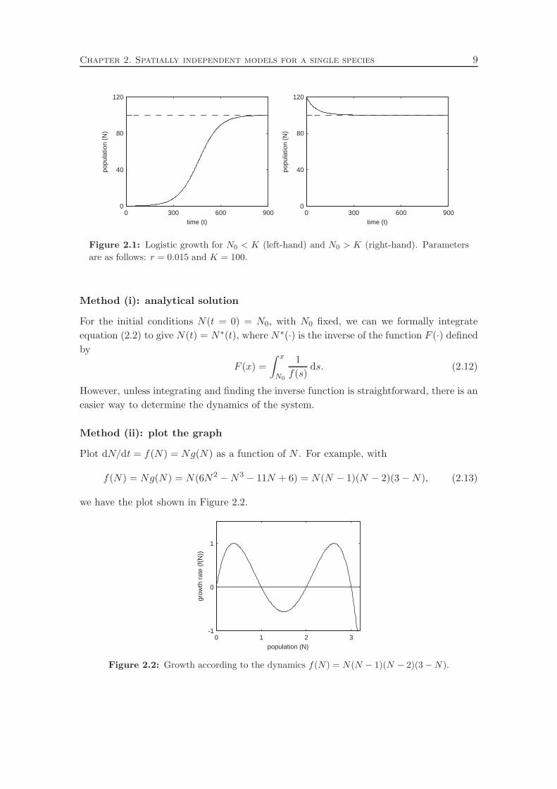
Sketching N(t) against time yields solution as plotted in Figure 2.1: we see that solutions
always monotonically relaxes to K as t→ ∞.
Aside. The logistic growth model has been observed to give very good fits to popula-
tion data in numerous, disparate, scenarios ranging from bacteria and yeast to rats and
sheep [8].
2.1.1 Investigating the dynamics
There are two techniques we can use to investigate the model
dN
dt= f(N) = Ng(N). (2.11)
Chapter 2. Spatially independent models for a single species 9
0 300 600 9000
40
80
120
time (t)
popu
latio
n (N
)
0 300 600 9000
40
80
120
time (t)
popu
latio
n (N
)
Figure 2.1: Logistic growth for N0 < K (left-hand) and N0 > K (right-hand). Parameters
are as follows: r = 0.015 and K = 100.
Method (i): analytical solution
For the initial conditions N(t = 0) = N0, with N0 fixed, we can we formally integrate
equation (2.2) to give N(t) = N∗(t), where N∗(·) is the inverse of the function F (·) definedby
F (x) =
∫ x
N0
1
f(s)ds. (2.12)
However, unless integrating and finding the inverse function is straightforward, there is an
easier way to determine the dynamics of the system.
Method (ii): plot the graph
Plot dN/dt = f(N) = Ng(N) as a function of N . For example, with
f(N) = Ng(N) = N(6N2 −N3 − 11N + 6) = N(N − 1)(N − 2)(3 −N), (2.13)
we have the plot shown in Figure 2.2.
0 1 2 3-1
0
1
population (N)
grow
th r
ate
(f(N
))
Figure 2.2: Growth according to the dynamics f(N) = N(N − 1)(N − 2)(3−N).

Chapter 2. Spatially independent models for a single species 10
Note 1. For a given initial condition, N0, the system will tend to the nearest root of
f(N) = Ng(N) in the direction of f(N0). The value of |N(t)| will tend to infinity with
large time if no such root exists.
For f(N) = Ng(N) = N(N − 1)(N − 2)(3 −N), we have:
• when N0 ∈ (0, 2] the large time asymptote is N(∞) = 1;
• for N0 > 2 the large time asymptote is N(∞) = 3;
• N(t) = 0 ∀t if N(0) = 0.
Note 2. On more than one occasion we will have a choice between using a graphical
method and an analytical method, as seen above. The most appropriate method to use
is highly dependent on context. The graphical method, Method (ii), quickly and simply
gives the large time behaviour of the system and stability information (see below). The
analytical method, Method (i), is often significantly more cumbersome, but yields all
information, at a detailed quantitative level, about the system.
Definition. A stationary point, also known as an equilibrium point, is a point where
the dynamics does not change in time. Thus in our specific context of dN/dt = f(N) =
Ng(N), the stationary points are the roots of f(N) = 0.
Example. For dN/dt = f(N) = Ng(N) = N(N − 1)(N − 2)(3 − N), the stationary
points are
N = 0, 1, 2, 3. (2.14)
Definition. A stationary point is stable if a solution starting sufficiently close to the
stationary point remains close to the stationary point.
Non-examinable. A rigorous definition is as follows. Let NN0(t) denote the solution
to dN/dt = f(N) = Ng(N) with initial condition N(t = 0) = N0. A stationary point,
Ns, is stable if, and only if, for all ǫ > 0 there exists a δ such that if |Ns −N0| < δ then
|NN0(t)−Ns| < ǫ.
Exercise. Use Figure 2.2 to deduce which of stationary points of the system
dN
dt= f(N) = Ng(N) = N(N − 1)(N − 2)(3 −N), (2.15)
are stable.
Solution. Figure 2.2 shows that both Ns = 1 and Ns = 3 are stable.

Chapter 2. Spatially independent models for a single species 11
2.1.2 Linearising about a stationary point
Suppose Ns is a stationary point of dN/dt = f(N) and make a small perturbation about
Ns:
N(t) = Ns + n(t), n(t) ≪ Ns. (2.16)
We have, by using a Taylor expansion of f(N) and denoting ′ = d/dN , that
f(N(t)) = f(Ns + n(t)) = f(Ns) + n(t)f ′(Ns) +1
2n(t)2f ′′(Ns) + . . . , (2.17)
and hence
dn
dt=dN
dt= f(N(t)) = f(Ns) + n(t)f ′(Ns) +
1
2n(t)2f ′′(Ns) + . . . (2.18)
The linearisation of dN/dt = f(N) about the stationary point Ns is given by neglecting
higher order (and thus smaller) terms to give
dn
dt= f ′(Ns)n(t).
The solution to this linear system is simply
n(t) = n(t = 0) exp
[
tdf
dN(Ns)
]
. (2.19)
Definition. Let Ns denote a stationary point of dN/dt = f(N), and let
n(t) = n(t = 0) exp
[
tdf
dN(Ns)
]
, (2.20)
be the solution of the linearisation about Ns. Then Ns is linearly stable if n(t) → 0 as
t→ ∞. In other words, Ns is linearly stable if
df
dN(Ns) < 0. (2.21)
Exercise. By algebraic means, deduce which stationary points of the system
dN
dt= f(N) = Ng(N) = N(N − 1)(N − 2)(3−N), (2.22)
are linearly stable. Can your answer be deduced graphically?
Solution. Differentiating f(N) with respect to N gives
f ′(N) = 2− 22N + 18N2 − 4N3, (2.23)
and hence f ′(0) = 6 (unstable), f ′(1) = −8 (stable) etc.
Consider the graph of f(N) to deduce stability graphically—steady states with negative
gradient are linearly stable c.f. Figure 2.2.

Chapter 2. Spatially independent models for a single species 12
0 1 2-1
0
1
population (N)
grow
th r
ate
(f(N
))
Figure 2.3: Growth according to the dynamics f(N) = (1−N)3.
Exercise. Find a function f(N) such that dN/dt = f(N) has a stationary point which
is stable and not linearly stable.
Solution. The function
f(N) = (1−N)3, (2.24)
gives f ′(1) = 0 and is therefore not linearly stable (see Figure 2.3).
2.1.3 Insect outbreak model
First introduced by Ludwig in 1978, the model supposes budworm population dynamics
to be modelled by the following equation:
dN
dt= rBN
(
1− N
KB
)
− p(N), p(N)def=
BN2
A2 +N2. (2.25)
The function p(N) is taken to represent the effect upon the population of predation by
birds. Plotting p(N) as a function of N gives the graph shown in Figure 2.4.
0 250 5000.0
0.1
0.2
0.3
0.4
0.5
population (N)
pred
atio
n ra
te (
p(N
))
Figure 2.4: Predation, p(N), in the insect outbreak model. Parameters are as follows:
A = 150, B = 0.5.

Chapter 2. Spatially independent models for a single species 13
Non-dimensionsionalisation
Let
N = N∗u, t = Tτ, (2.26)
where N∗, N have units of biomass, and t, T have units of time, with N∗, T constant.
Then
N∗
T
du
dτ= rBN
∗u
(
1− N∗u
KB
)
− B(N∗)2u2
A2 + (N∗)2u2, (2.27)
⇒ du
dτ= rBTu
(
1− N∗u
KB
)
− BTN∗u2
A2 + (N∗)2u2. (2.28)
Hence with
N∗ = A, T =A
B, r = rBT =
rBA
B, q =
KB
N∗=KB
A, (2.29)
we havedu
dτ= ru
(
1− u
q
)
− u2
1 + u2def= f(u; r, q). (2.30)
Thus we have reduced the number of parameters in our model from four to two, which
substantially simplifies our subsequent study.
Steady states
The steady states are given by the solutions of
ru
(
1− u
q
)
− u2
1 + u2= 0. (2.31)
Clearly u = 0 is a steady state. We proceed graphically to consider the other steady states
which are given by the intersection of the graphs
f1(u) = r
(
1− u
q
)
and f2(u) =u
1 + u2. (2.32)
The top left plot of Figure 2.5 shows plots of f1(u) and f2(u) for different values of r and
q. We see that, depending on the values of r and q, we have either one or three non-zero
steady states. Noting thatdf(u; r, q)
du
∣∣∣∣u=0
= r > 0, (2.33)
typical plots of du/dτ vs. u are shown in Figure 2.5 for a range of values of r and q.
Definition. A system displaying hysteresis exhibits a response to the increase of a
driving variable which is not precisely reversed as the driving variable is decreased.
Remark. Hysteresis is remarkably common. Examples include ferromagnetism and
elasticity, amongst others. See http://en.wikipedia.org/wiki/Hysteresis for more
details.

Chapter 2. Spatially independent models for a single species 14
0 10 200.0
0.2
0.4
0.6
scaled population (u)
f 1(u)
/ f2(u
)
0 5 10-0.2
0.0
0.2
scaled population (u)
f(u;
r,q)
0 5 10-0.2
0.0
0.2
scaled population (u)
f(u;
r,q)
0 5 10
0.0
0.2
0.4
0.6
scaled population (u)
f(u;
r,q)
Figure 2.5: Dynamics of the non-dimensional insect outbreak model. Top left: plots of
the functions f1(u) (dashed line) and f2(u) (solid line) with parameters r = 0.2, 0.4, 0.6,
q = 10, 15, 20, respectively. Top right: plot of f(u; r, q) with parameters r = 0.6, q = 0.6.
Bottom left: plot of f(u; r, q) with parameters r = 0.6, q = 6. Bottom right: plot of f(u; r, q)
with parameters r = 0.6, q = 10.
Extended Exercise
• Fix r = 0.6. Explain how the large time asymptote of u, and hence N , changes as
one slowly increases q from q ≪ 1 to q ≫ 1 and then one decreases q from q ≫ 1 to
q ≪ 1. In particular, show that hysteresis is present. Note for this value of r, there
are three non-zero stationary points for q ∈ (q1, q2) with 1 < q1 < q2 < 10.
Solution. For small values of q there is only one non-zero steady state, S1. As q is
increased past q1, three non-zero steady states exist, S1, S2, S3, but the system stays
at S1. As q is increased further, past q2, the upper steady state S3 is all that remains
and hence the system moves to S3. If q is now decreased past q2, three non-zero
steady states (S1, S2, S3) exist but the system remains at S3 until q is decreased
past q1.
Figure 2.6 shows f(u; r, q) for different values of q. The dashed line shows a plot for
q = q1 whilst the dash-dotted line shows a plot for q = q2.
• What is the biological interpretation of the presence of hysteresis in this model?

Chapter 2. Spatially independent models for a single species 15
0 5 10-0.4
-0.2
0.0
0.2
0.4
scaled population (u)
du/d
τ
5.5 6.0 6.5 7.00
1
2
3
4
5
q
u*
Figure 2.6: Left-hand plot: du/dτ = f(u; r, q) in the non-dimensional insect outbreak model
as q is varied. For small q there is one, small, steady state, for q ∈ (q1, q2) there are three
non-zero steady states and for large q there is one, large, steady state. Right-hand plot: the
steady states plotted as a function of the parameter q reveals the hysteresis loop.
Solution. If the carrying capacity, q, is accidentally manipulated such that an out-
break occurs (S1 → S3) then reversing this change is not sufficient to reverse the
outbreak.
2.1.4 Harvesting a single natural population
We wish to consider a simple model for the maximum sustainable yield. Suppose, in the
absence of harvesting, we have
dN
dt= rN
(
1− N
K
)
. (2.34)
We consider a perturbation from the non-zero steady state, N = K. Thus we write
N = K + n, and find, on linearising,
dn
dt= −rn ⇒ n = n0e
−rt. (2.35)
Hence the system returns to equilibrium on a timescale of TR(0) = O(1/r).
We consider two cases for harvesting:
• constant yield, Y ;
• constant effort, E.
Constant yield
For a constant yield, Y = Y0, our equations are
dN
dt= rN
(
1− N
K
)
− Y0def= f(N ;Y0). (2.36)

Chapter 2. Spatially independent models for a single species 16
0 25 50 75 100-0.3
-0.2
-0.1
0.0
0.1
0.2
0.3
population (N)
f Y0(N
)
Figure 2.7: Dynamics of the constant yield model for Y0 = 0.00, 0.15, 0.30. As Y0 is increased
beyond a critical value the steady states disappear and N → 0 in finite time. Parameters are
as follows: K = 100 and r = 0.01.
Plotting dN/dt as a function of N reveals (see Figure 2.7) that the steady states disappear
as Y0 is increased beyond a critical value, and then N → 0 in finite time.
The steady states are given by the solutions of
rN∗ − rN∗2
K− Y0 = 0 ⇒ N∗ =
r ±√
r2 − 4rY0/K
2r/K. (2.37)
Therefore extinction will occur once
Y0 >rK
4. (2.38)
Constant effort
For harvesting at constant effort our equations are
dN
dt= rN
(
1− N
K
)
− ENdef= f(N ;E) = N(r − E)− rN2
K, (2.39)
where the yield is Y (E) = EN . The question is: how do we maximise Y (E) such that the
stationary state still recovers?
The steady states, N∗, are such that f(N∗;E) = 0 (see Figure 2.8). Thus
N∗(E) =(r −E)K
r=
(
1− E
r
)
K, (2.40)
and hence
Y ∗(E) = EN∗(E) =
(
1− E
r
)
KE. (2.41)
Thus the maximum yield, and corresponding value of N∗, are given by the value of E such
that∂Y ∗
∂E= 0 ⇒ E =
r
2, Y ∗
max =rK
4, N∗
max =K
2. (2.42)

Chapter 2. Spatially independent models for a single species 17
Linearising about the stationary state N∗(E) we have N = N∗(E) + n with
dn
dt≃ fE(N
∗) +df(N ;E)
dN
∣∣∣∣N=N∗
n+ . . . = −(r − E)n + . . . , (2.43)
and hence the recovery time is given by
TR(E) ≃ O(
1
r − E
)
. (2.44)
Defining the recovery time to be the time for a perturbation to decrease by a factor of e
according to the linearised equations about the non-zero steady state, then
TR(0) =1
r, TR(E) =
1
r − E. (2.45)
Hence, at the maximum yield state,
TR(E) =2
rsince E =
r
2at maximum yield. (2.46)
As we measure Y it is useful to rewrite E in terms of Y to give the ratio of recovery times
in terms of the yield Y (E) and the maximum yield YM :
TR(Y )
TR(0)=
2
1±√
1− YYM
. (2.47)
Derivation. At steady state, we have
K
rE2 −KE + Y ∗ = 0 as Y ∗ = EN∗ = KE
(
1− E
r
)
. (2.48)
This gives
E =r ± r
√
1− 4Y ∗/Kr
2⇒ r − E =
r
2
[
1∓√
1− Y ∗
Y ∗M
]
. (2.49)
Substituting into equation (2.45) gives the required result.
Plotting TR(Y )/TR(0) as a function of Y/YM yields some interesting observations, as
shown in Figure 2.8.
Note. As TR increases the population recovers less quickly, and therefore spends more
time away from the steady state, N∗. The biological implication is that, in order to
maintain a constant yield, E must be increased. This, in turn, implies TR increases,
resulting in a positive feedback loop that can have disastrous consequences upon the
population.

Chapter 2. Spatially independent models for a single species 18
0 25 50 75 1000.0
0.1
0.2
0.3
population (N)
0.0 0.2 0.4 0.6 0.8 1.00
5
10
15
Y / YM
TR(Y
) / T
R(0
)
Figure 2.8: Dynamics of the constant effort model. The left-hand plot shows the logistic
growth curve (solid line) and the yield, Y = EN (dashed lines), for two values of E. The
right-hand plot shows the ratio of recovery times, TR(Y )/TR(0), with the negative root plotted
as a dashed line and the positive root as a solid line. Parameters are as follows: K = 100 and
r = 0.01.
2.2 Discrete population models for a single species
When there is no overlap in population numbers between each generation, we have a
discrete model:
Nt+1 = Ntf(Nt) = H(Nt). (2.50)
A simple example is
Nt+1 = rNt, (2.51)
which implies
Nt = rtN0 →
∞ r > 1
N0 r = 1
0 r < 1
. (2.52)
Definition. An equilibrium point, N∗, for a discrete population model satisfies
N∗ = N∗f(N∗) = H(N∗). (2.53)
Such a point is often known as a fixed point.
An extension of the simple model, equation (2.51), called the Ricker model includes a
reduction of the growth rate for large Nt:
Nt+1 = Nt exp
[
r
(
1− Nt
K
)]
, r > 0 K > 0, (2.54)
or, in non-dimensionalised form,
ut+1 = ut exp [r (1− ut)]def= H(ut). (2.55)
We can start developing an idea of how this system evolves in time via cobwebbing, a
graphical technique, as shown in Figure 2.9.

Chapter 2. Spatially independent models for a single species 19
0 50 100 150 2000
50
100
150
Nt
Nt+
1
0 2 4 6 8 100
30
60
90
120
generation (t)
popu
latio
n (N
t)
Figure 2.9: Dynamics of the Ricker model. The left-hand plot shows a plot of Nt+1 =
Nt exp [r (1−Nt/K)] alongside Nt+1 = Nt with the cobwebbing technique shown. The right-
hand plot shows Nt for successive generation times t = 1, 2, . . . , 10. Parameters are as follows:
N0 = 5, r = 1.5 and K = 100.
In particular, it is clear that the behaviour sufficiently close to a fixed point, u∗, depends
on the value of H ′(u∗). For example:
• −1 < H ′(u∗) < 0
• H ′(u∗) = −1

Chapter 2. Spatially independent models for a single species 20
• H ′(u∗) < −1
2.2.1 Linear stability
More generally, to consider the stability of an equilibrium point algebraically, rather than
graphically, we write
ut = u∗ + vt, (2.56)
where u∗ is an equilibrium value. Note that u∗ is time-independent and satisfies u∗ =
H(u∗). Hence
ut+1 = u∗ + vt+1 = H(u∗ + vt) = H(u∗) + vtH′(u∗) + o(v2t ). (2.57)
Consequently, we have
vt+1 = H ′(u∗)vt where H ′(u∗) is a constant, independent of t, (2.58)
and thus
vt =[H ′(u∗)
]tv0. (2.59)
This in turn enforces stability if |H ′(u∗)| < 1 and instability if |H ′(u∗)| > 1.
Definition. A discrete population model is linearly stable if |H ′(u∗)| < 1.
2.2.2 Further investigation
The equations are not as simple as they seem. For example, from what we have seen thus
far, the discrete time logistic model seems innocuous enough.
Nt+1 = rNt
(
1− Nt
K
)
, r > 0 K > 0. (2.60)
If we put in enough effort, one could be forgiven for thinking that the use of cobwebbing
will give a simple representation of solutions of this equation. However, the effects of
increasing r are stunning. Figure 2.10 shows examples of cobwebbing when r = 1.5 and
r = 4.0.
It should now be clear that even this simple equation does not always yield a simple
solution! How do we investigate such a complicated system in more detail?

Chapter 2. Spatially independent models for a single species 21
0 20 40 60 80 1000
10
20
30
40
Nt
Nt+
1
0 20 40 60 80 1000
50
100
Nt
Nt+
1
Figure 2.10: Dynamics of the discrete logistic model. The left-hand plot shows results for
r = 1.5 whilst the right-hand plot shows results for r = 4.0. Other parameters are as follows:
N0 = 5 and K = 100.
Definition. A bifurcation point is, in the current context, a point in parameter space
where the number of equilibrium points, or their stability properties, or both, change.
We proceed to take a closer look at the non-dimensional discrete logistic growth model:
ut+1 = rut (1− ut) = H(ut), (2.61)
for different values of the parameter r, and, in particular, we seek the values where the
number or stability nature of the equilibrium points change. Note that we have equilibrium
points at u∗ = 0 and u∗ = (r − 1)/r, and that H ′(u) = r − 2ru.
For 0 < r < 1, we have:
• u∗ = 0 is a stable steady state since |H ′(0)| = |r| < 1;
• the equilibrium point at u∗ = (r − 1)/r is unstable. It is also unreachable, and thus
irrelevant, for physical initial conditions with u0 ≥ 0.
For 1 < r < 3 we have:
• u∗ = 0 is an unstable steady state since |H ′(0)| = |r| > 1;
• u∗ = (r − 1)/r is an stable steady state since |H ′((r − 1)/r)| = |2− r| < 1.
In Figure 2.11 we plot this on a diagram of steady states, as a function of r, with stable
steady states indicated by solid lines and unstable steady states by dashed lines.
When r = 1 we have (r − 1)/r = 0, so both equilibrium points are at u∗ = 0, with
H ′(u∗ = 0) = 1. Clearly we have a switch in the stability properties of the equilibrium
points, and thus r = 1 is a bifurcation point.

Chapter 2. Spatially independent models for a single species 22
0 1 2 3
0.0
0.2
0.4
0.6
0.8
r
u*
Figure 2.11: Bifurcation diagram for the non-dimensional discrete logistic model. The non-
zero steady state is given, for r > 1, by N∗ = (r − 1)/r.
What happens for r > 3? We have equilibrium points at u∗ = 0, u = (r − 1)/r and
H ′(u∗ = (r − 1)/r) < −1; both equilibrium points are unstable. Hence if the system
approaches one of these equilibrium points the approach is only transient; it quickly moves
away. We have a switch in the stability properties of the equilibrium points, and thus r = 3
is a bifurcation point.
To consider the dynamics of this system once r > 3 we consider
ut+2 = H(ut+1) = H [H(ut)]def= H2(ut) = r [rut(1− ut)] [1− rut(1− ut)] . (2.62)
Figure 2.12 shows H2(ut) for r = 2.5 and r = 3.5 and demonstrates the additional steady
states that arise as r is increased past r = 3.
0.0 0.2 0.4 0.6 0.8 1.00.0
0.2
0.4
0.6
0.8
1.0
ut
u t+2
0.0 0.2 0.4 0.6 0.8 1.00.0
0.2
0.4
0.6
0.8
1.0
ut
u t+2
Figure 2.12: Dynamics of the non-dimensional discrete logistic model in terms of every
second iteration. The left-hand plot shows results for r = 2.5 whilst the right-hand plot shows
results for r = 3.5.
Note. The fixed points of H2 satisfy u∗2 = H2(u∗2), which is a quartic equation in u∗2.
However, we know two solutions, the fixed pointsH(·), i.e. 0 and (r−1)/r. Using standard

Chapter 2. Spatially independent models for a single species 23
techniques we can reduce the quartic to a quadratic, which can be solved to reveal the
further fixed points of H2, namely
u∗2 =r + 1
2r± 1
2r
[(r − 1)2 − 4
]1/2. (2.63)
These roots exist if (r − 1)2 > 4, i.e. r > 3.
Definition. The mth composition of the function H is given by
Hm(u)def= [H ·H . . .H ·H]︸ ︷︷ ︸
m times
(u). (2.64)
Definition. A point u is periodic of period m for the function H if
Hm(u) = u, Hi(u) 6= u, i ∈ 1, 2, . . . m− 1. (2.65)
Thus the points
u∗2 =r + 1
2r± 1
2r
[(r − 1)2 − 4
]1/2, (2.66)
are points of period 2 for the function H.
Problem. Show that the u∗2 are stable with respect to the function H2 for r > 3,
(r − 3) ≪ 1.
Let
u0def=
r + 1
2r± 1
2r
[(r − 1)2 − 4
]1/2, u1 = H(u0), u2 = H2(u0), (2.67)
and let
λ =∂
∂u[H2(u)] |u=u0
. (2.68)
Then
λ =∂
∂u[H ·H(u)] |u=u0
= H ′(u0)H′(u1). (2.69)
Thus for stability we require |H ′(u0)H′(u1)| < 1.
Exercise. Finish the problem: show that the steady states
u∗2 =r + 1
2r± 1
2r
[(r − 1)2 − 4
]1/2, (2.70)
are stable for the dynamical system ut+1 = H2(ut), with r > 3, (r − 3) ≪ 1.

Chapter 2. Spatially independent models for a single species 24
Exercise. Suppose u0 is an equilibrium point of period m for the function H. Show
that u0 is stable if
Πm−1i=0
[H ′(ui)
]< 1, (2.71)
where ui = Hi(u0) for i ∈ 1, 2, . . . ,m− 1.
Solution. Defining λ in a similar manner as before, we have
λ =∂
∂uHm(u)
∣∣∣∣u=u0
, (2.72)
=∂
∂u[H(Q(u)]
∣∣∣∣u=u0
, where Q(u) = Hm−1(u), (2.73)
= H ′(Q(u))∂Q
∂u
∣∣∣∣u=u0
, (2.74)
= H ′(um−1)∂
∂uHm−1
∣∣∣∣u=u0
. (2.75)
Hence, by iteration, we have the result.
We plot the fixed points of H2, which we now know to be stable, in addition to the fixed
points of H1, in Figure 2.13. The upper branch, u∗2U , is given by the positive root of
equation (2.70) whilst the lower branch, u∗2L, is given by the negative root. We have
u∗2L = H(u∗2U ), u∗2U = H(u∗2L). Thus a stable, period 2, oscillation is present, at least for
(r − 3) ≪ 1. Any solution which gets sufficiently close to either u∗2U or u∗2L stays close.
0 1 2 3
0.0
0.2
0.4
0.6
0.8
1.0
r
u*
Figure 2.13: Bifurcation diagram for the non-dimensional discrete logistic model with inclu-
sion of the period 2 solutions.
For higher values of r, there is a bifurcation point for H2; we can then find a stable
fixed point for H4(u) : : H2[H2(u)] in a similar manner. Increasing r further there is a
bifurcation point for H4(u). Again, we are encountering a level of complexity which is too
much to deal with our current method.
To bring further understanding to this complex system, we note the following definition.

Chapter 2. Spatially independent models for a single species 25
Definition. An orbit generated by the point u0 are the points u0, u1, u2, , u3, . . .where ui = Hi(u) = H(ui−1).
We are primarily interested in the large time behaviour of these systems in the context of
biological applications. Thus, for a fixed value of r, we start with a reasonable initial seed,
say u∗ = 0.5, and plot the large time asymptote of the orbit of u∗, ie. the points Hi(u∗)
once i is sufficiently large for there to be no transients. This gives an intriguing plot; see
Figure 2.14.
3.0 3.2 3.4 3.6 3.8 4.00.0
0.2
0.4
0.6
0.8
1.0
r
u*
Figure 2.14: The orbit diagram of the logistic map. For each value of r ∈ [3, 4] along
horizontal axis, points on the large time orbits of the logistic map are plotted.
In particular, we have regions where, for r fixed, there are three points along the ver-
tical corresponding to period 3 oscillations. This means any period of oscillation exists
and we have a chaotic system. This can be proved using Sharkovskii’s theorem. See P.
Glendinning, Stability, Instability and Chaos [4] for more details on chaos and chaotic
systems.
Note. A common discrete population model in mathematical biology is
Nt+1 =rNt
1 + aN bt
. (2.76)
Models of this form for the Colorado beetle are within the periodic regimes, while Nichol-
son’s blowfly model is in the chaotic regime [8].
2.2.3 The wider context
In investigating the system
ut+1 = rut (1− ut)def= H(ut), (2.77)
we have explored a very simple equation which, in general, exhibits greatly different be-
haviours with only a small change in initial conditions or parameters (i.e. linear growth
rate, r). Such sensitivity is a hallmark feature of chaotic dynamics. In particular, it makes
Chapter 2. Spatially independent models for a single species 26
prediction very difficult. There will always be errors in a model’s formalism, initial condi-
tions and parameters and, in general, there is no readily discernible pattern in the way the
model behaves. Thus, assuming the real system behaviour is also chaotic, using statistical
techniques to extract a pattern of behaviour to thus enable an extrapolation to predict
future behaviour is also fraught with difficulty. Attempting to make accurate predictions
with models containing chaos is an active area of research, as is developing techniques to
analyse seemingly random data to see if such data can be explained by a simple chaotic
dynamical system.
Chapter 3
Continuous population models:
interacting species
In this chapter we consider interacting populations, but again in the case where spatial
variation is not important. Appendix A contains relevant information for phase plane
analysis that may be useful.
References.
• J. D. Murray, Mathematical Biology, 3rd edition, Volume I, Chapter 3 [8].
• L. Edelstein-Keshet, Mathematical Models in Biology, Chapter 6 [2].
• N. F. Britton, Essential Mathematical Biology, Chapter 2 [1].
There are three main forms of interaction:
Predator-prey An upsurge in population I (prey) induces a growth in population II
(predator). An upsurge in population II (predator) induces a decline in population
I (prey).
Competition An upsurge in either population induces a decline in the other.
Symbiosis An upsurge in either population induces an increase in the other.
Of course, there are other possible interactions, such as cannibalism, especially with the
“adult” of a species preying on the young, and parasitism.
3.1 Predator-prey models
The most common predator-prey model is the Lotka-Volterra model. With N the number
of prey and P the number of predators, this model can be written
dN
dt= aN − bNP, (3.1)
dP
dt= cNP − dP, (3.2)
27

Chapter 3. Continuous population models: interacting species 28
with a, b, c, d positive parameters and c < b. Non-dimensionalising with u = (c/d)N ,
v = (b/a)P , τ = at and α = d/a, we have
1
1/a
d
c
du
dτ=ad
cu− bd
c
a
buv ⇒ du
dτ= u− uv = u(1− v) ≡ f(u, v), (3.3)
1
1/a
a
b
dv
dτ= c
d
c
a
buv − d
a
bv, ⇒ dv
dτ= α(uv − v) = αv(u− 1) ≡ g(u, v), (3.4)
There are stationary points at (u, v) = (0, 0) and (u, v) = (1, 1).
Exercise. Find the stability of the stationary points (u, v) = (0, 0) and (u, v) = (1, 1).
The Jacobian, J , is given by
J =
(
fu fvgu gv
)
=
(
1− v −uαv α(u− 1)
)
. (3.5)
At (0, 0) we have
J =
(
1 0
0 −α
)
, (3.6)
with eigenvalues 1, −α. Therefore the steady state (0, 0) is an unstable saddle.
At (1, 1) we have
J =
(
0 −1
α 0
)
, (3.7)
with eigenvalues ±i√α. Therefore the steady state (1, 1) is a centre (not linearly stable).
These equations are special; we can integrate them once, as follows, to find a conserved
constant:du
dv=
u(1 − v)
α(u− 1)v⇒
∫u− 1
udu =
∫1− v
αv. (3.8)
Hence
H = const = αu+ v − α lnu− ln v. (3.9)
This can be rewritten as (ev
v
)(eu
u
)α
= eH , (3.10)
from which we can rapidly deduce that the trajectories in the (u, v) plane take the form
shown in Figure 3.1. Thus u and v oscillate in time, though not in phase, and hence we
have a prediction; predators and prey population numbers oscillate out of phase. There
are often observations of this e.g. hare-lynx interactions.

Chapter 3. Continuous population models: interacting species 29
0.0 1.0 2.0 3.0 4.0 5.00.0
1.0
2.0
3.0
4.0
5.0
u
v
0 4 8 12 160.0
1.0
2.0
Time
popu
latio
n
uv
Figure 3.1: Dynamics of the non-dimensional Lotka-Volterra system for α = 1.095 and
H = 2.1, 2.4, 3.0, 4.0. The left-hand plot shows the dynamics in the (u, v) phase plane whilst
the right-hand plot shows the temporal evolution of u and v.
3.1.1 Finite predation
The common predator-prey model assumes that as N → ∞ the rate of predation per
predator becomes unbounded, as does the rate of increase of the predator’s population.
However, with an abundance of food, these quantities will saturate rather than become
unbounded. Thus, a more realistic incorporation of an abundance of prey requires a refine-
ment of the Lotka-Volterra model. A suitable, simple, model for predator-prey interactions
under such circumstances would be (after a non-dimensionalisation)
du
dτ= f(u, v) = u(1− u)− auv
d+ u, (3.11)
dv
dτ= g(u, v) = bv
(
1− v
u
)
, (3.12)
where a, b, d are positive constants. Note the effect of predation per predator saturates
at high levels of u whereas the predator levels are finite at large levels of prey and drop
exceedingly rapidly in the absence of prey.
There is one non-trivial equilibrium point, (u∗, v∗), satisfying
v∗ = u∗ where (1− u∗) =au∗
d+ u∗, (3.13)
and hence
u∗ =1
2
[
−(a+ d− 1) +√
(a+ d− 1)2 + 4d]
. (3.14)
The Jacobian at (u∗, v∗) is
J =
(
fu fvgu gv
)∣∣∣∣∣(u∗,v∗)
, (3.15)
where
fu(u∗, v∗) = 1− 2u∗ − au∗
d+ u∗+
au∗v∗
(d+ u∗)2= −u∗ + a(u∗)2
(d+ u∗)2. (3.16)

Chapter 3. Continuous population models: interacting species 30
fv(u∗, v∗) = − au∗
d+ u∗, (3.17)
gu(u∗, v∗) =
b(v∗)2
(u∗)2= b, (3.18)
gv(u∗, v∗) = b
(
1− 2v∗
u∗
)
= −b. (3.19)
The eigenvalues satisfy
(λ− fu)(λ− gv)− fvgu = 0 ⇒ λ2 − (fu + gv)λ+ (fugv − fvgu) = 0, (3.20)
and hence
λ2 − αλ+ β = 0 ⇒ λ =α±
√
α2 − 4β
2, (3.21)
where
α = −u∗ + a(u∗)2
(u∗ + d)2− b, β = b
(
u∗ − a(u∗)2
(u∗ + d)2− (u∗ − 1)
)
. (3.22)
Note that
β = 1− a(u∗)2
(u∗ + d)2= 1− u∗(1− u∗)
(u∗ + d)=
(u∗ + d)− u∗ + (u∗)2
u∗ + d=d+ (u∗)2
d+ u∗> 0. (3.23)
Thus, if α < 0 the eigenvalues λ are such that we have either:
• a stable node (α2 − 4β > 0);
• stable focus (α2 − 4β < 0);
at the equilibrium point (u∗, v∗).
If α > 0 we have an unstable equilibrium point at (u∗, v∗).
3.2 A look at global behaviour
This previous section illustrated local dynamics: we have conditions for when the dynamics
will stably remain close to the non-trivial equilibrium point. One is also often interested
in the global dynamics. However, determining the global dynamics of a system, away
from its equilibrium points, is a much more difficult problem compared to ascertaining the
local dynamics, sufficiently close to the equilibrium points. For specific parameter values,
one can readily solve the ordinary differential equations to consider the behaviour of the
system. One is also interested in the general properties of the global behaviour. This is
more difficult, and we will consider one possible approach below.
There are many potential tools available: nullcline analysis, the Poincare-Bendixson The-
orem, the Poincare Index and the Bendixson-Dulac Criterion. The Poincare-Bendixson
Theorem is a useful tool for proving that limit cycles must exist, while Poincare indices
and the Bendixson-Dulac Criterion are useful tools for proving a limit cycle cannot exist.

Chapter 3. Continuous population models: interacting species 31
We will briefly consider nullclines and the Poincare-Bendixson Theorem in detail. Please
refer to P. Glendinning, Stability, Instability and Chaos: An Introduction to the Theory
of Nonlinear Differential Equations [4], or D. W. Jordan and P. Smith, Mathematical
Techniques: An Introduction for Engineering, Mathematical and Physical Sciences [6], for
further details than considered here.
3.2.1 Nullclines
Definition. Consider the equations
du
dt= f(u, v),
dv
dt= g(u, v). (3.24)
The nullclines are the curves in the phase plane where f(u, v) = 0 and g(u, v) = 0.
Reconsider
du
dτ= f(u, v) = u(1− u)− auv
d+ u, (3.25)
dv
dτ= g(u, v) = bv
(
1− v
u
)
. (3.26)
The u nullclines are given by
f(u, v) ≡ 0 ⇒ u ≡ 0 and v =1
a(1− u)(u+ d). (3.27)
The v nullclines are given by
g(u, v) ≡ 0 ⇒ v ≡ 0 and v = u. (3.28)
A sketch of the nullclines and the behaviour of the phase plane trajectories is shown in
Figure 3.2.
3.2.2 The Poincare-Bendixson Theorem
For a system of two first order ordinary differential equations, consider a closed bounded
region D. Suppose a positive half path, H, lies entirely within D. Then one of the
following is true:
1. H is a closed trajectory, e.g. a limit cycle;
2. H asymptotically tends to a closed trajectory, e.g. a limit cycle;
3. H terminates on a stationary point.
Therefore, if D does not have a stationary point then there must be a limit cycle.
For a proof see P. Glendinning, Stability, Instability and Chaos: An Introduction to the
Theory of Nonlinear Differential Equations [4].

Chapter 3. Continuous population models: interacting species 32
0.0 0.2 0.4 0.6 0.8 1.00.0
0.2
0.4
0.6
0.8
1.0
u
v
Figure 3.2: The (u, v) phase-plane for the finite predation model when the steady state is
stable. The u nullclines are plotted in red and the v nullclines in green. Trajectories for a
number of different initial conditions are shown as dashed lines. Parameters are as follows:
a = 2.0, b = 0.1, d = 2.0.
Exercise. Explain why α > 0 in the previous example (see equation (3.22)) implies
we have limit cycle dynamics. What does this mean in terms of the population levels of
predator and prey?
Solution. For α > 0 the steady state is an unstable node or spiral. Further, we can find a
simple, closed boundary curve, C, in the positive quadrant of the (u, v) plane, such that
on C phase trajectories always point into the domain, D, enclosed by C. Applying the
Poincare-Benedixon Theorem to the domain gives the existence of a limit cycle. See J. D.
Murray, Mathematical Biology Volume I [8] (Chapter 3.4) for more details.
3.3 Competitive exclusion
We consider an ordinary differential equation model of two competitors. An example might
be populations of red squirrels and grey squirrels [8]. Here, both populations compete for
the same resources and a typical model for their dynamics is
dN1
dt= r1N1
(
1− N1
K1− b12
N2
K1
)
, (3.29)
dN2
dt= r2N2
(
1− N2
K2− b21
N1
K2
)
, (3.30)
where K1, K2, r1, r2, b12, b21 are positive constants. Let us associate N1 with red squirrels
and N2 with grey squirrels in our example.
In particular, given a range of parameter values and some initial values for N1 and N2 at
the time t = 0, we would typically like to know if the final outcome is one of the following
possibilities:
• the reds become extinct, leaving the greys;

Chapter 3. Continuous population models: interacting species 33
• the greys become extinct, leaving the reds;
• both reds and greys become extinct;
• the reds and greys co-exist. If this system is perturbed in any way will the reds and
greys continue to coexist?
After a non-dimensionalisation (exercise) we have
u′1 = u1(1− u1 − α12u2)def= f1(u1, u2), (3.31)
u′2 = ρu2(1− u2 − α21u1)def= f2(u1, u2), (3.32)
where ρ = r2/r1.
The stationary states are
(u∗1, u∗2) = (0, 0), (u∗1, u
∗2) = (1, 0), (u∗1, u
∗2) = (0, 1), (3.33)
and
(u∗1, u∗2) =
1
1− α12α21(1− α12, 1− α21), (3.34)
if α12 < 1 and α21 < 1 or α12 > 1 and α21 > 1.
The Jacobian is
J =
(
1− 2u1 − α12u2 −α12u1−ρα21u2 ρ(1− 2u2 − α21u1)
)
. (3.35)
It is a straightforward application of phase plane techniques to investigate the nature of
these equilibrium points:
Steady state (u∗1, u∗2) = (0, 0).
J− λI =
(
1− λ 0
0 ρ− λ
)
⇒ λ = 1, ρ. (3.36)
Therefore (0, 0) is an unstable node.
Steady state (u∗1, u∗2) = (1, 0).
J− λI =
(
−1− λ −α12
0 ρ(1− α21)− λ
)
⇒ λ = −1, ρ(1− α21). (3.37)
Therefore (1, 0) is a stable node if α21 > 1 and a saddle point if α21 < 1.
Steady state (u∗1, u∗2) = (0, 1).
J− λI =
(
1− α12 − λ 0
−ρα21 −ρ− λ
)
⇒ λ = −ρ, 1− α12. (3.38)
Therefore (0, 1) is a stable node if α12 > 1 and a saddle point if α12 < 1.

Chapter 3. Continuous population models: interacting species 34
Steady state (u∗1, u∗2) =
11−α12α21
(1− α12, 1− α21).
J− λI =1
1− α12α21
(
α21 − 1− λ α12(α12 − 1)
ρα21(α21 − 1) ρ(α21 − 1)− λ
)
. (3.39)
Stability depends on α12 and α21.
There are several different possible behaviours. The totality of all behaviours of the above
model is reflected in how one can arrange the nullclines within the positive quadrant.
However, for competing populations these straight line nullclines have negative gradients.
Figure 3.3 shows the model behaviour for different sets of parameter values.
0.0 0.4 0.8 1.20.0
0.4
0.8
1.2
u1
u 2
0.0 0.4 0.8 1.20.0
0.4
0.8
1.2
u1
u 2
0.0 0.4 0.8 1.20.0
0.4
0.8
1.2
u1
u 2
0.0 0.4 0.8 1.20.0
0.4
0.8
1.2
u1
u 2
Figure 3.3: Dynamics of the non-dimensional competitive exclusion system. Top left: α12 =
0.8 < 1, α21 = 1.2 > 1 and u2 is excluded. Top right: α12 = 1.2 > 1, α21 = 0.8 < 1 and u1 is
excluded. Bottom left: α12 = 1.2 > 1, α21 = 1.2 > 1 and exclusion is dependent on the initial
conditions. Bottom right: α12 = 0.8 < 1, α21 = 0.8 < 1 and we have coexistence. The stable
steady states are marked with ∗’s and ρ = 1.0 in all cases. The red lines indicate f1 ≡ 0 whilst
the green lines indicate f2 ≡ 0.
Note. In ecology the concept of competitive exclusion is that two species competing for
exactly the same resources cannot stably coexist. One of the two competitors will always
have an ever so slight advantage over the other that leads to extinction of the second
competitor in the long run (or evolution into distinct ecological niches).

Chapter 3. Continuous population models: interacting species 35
3.4 Mutualism (symbiosis)
We consider the same ordinary differential equation model for two competitors, i.e.
dN1
dt= r1N1
(
1− N1
K1+ b12
N2
K1
)
, (3.40)
dN2
dt= r2N2
(
1− N2
K2+ b21
N1
K2
)
, (3.41)
where K1, K2, r1, r2, b12, b21 are positive constants or, after non-dimensionalisation,
u′1 = u1(1− u1 + α12u2)def= f1(u1, u2), (3.42)
u′2 = ρu2(1− u2 + α21u1)def= f2(u1, u2). (3.43)
In symbiosis, the straight line nullclines will have positive gradients leading to the following
two possible behaviours shown in Figure 3.4.
0.0 0.4 0.8 1.20.0
0.4
0.8
1.2
u1
u 2
0.0 0.4 0.8 1.20.0
0.4
0.8
1.2
u1
u 2
Figure 3.4: Dynamics of the non-dimensional symbiotic system. The left-hand figure shows
population explosion (α12 = 0.6 = α21) whilst the right-hand figure shows population coex-
istence (α12 = 0.1 = α21). The stable steady states are marked with ∗’s and ρ = 1.0 in all
cases. The red lines indicate f1 ≡ 0 whilst the green lines indicate f2 ≡ 0.
3.5 Interacting discrete models
It is also possible, and sometimes useful, to consider interacting discrete models which
take the form
ut+1 = f(ut, vt), (3.44)
vt+1 = g(ut, vt), (3.45)
and possess steady states at the solutions of
u∗ = f(u∗, v∗), v∗ = g(u∗, v∗). (3.46)
It is interesting and relevant to study the linear stability of these equilibrium points, and
the global dynamics, but we do not have time to pursue this here.
Chapter 4
Enzyme kinetics
In this chapter we consider enzyme kinetics, which can be thought of as a particular case
of an interacting species model. In all cases here we will neglect spatial variation.
Throughout, we will consider the m chemical species C1, . . . , Cm.
• The concentration of Ci, denoted ci, is defined to be the number of molecules of Ci
per unit volume.
• A standard unit of concentration is moles m−3, often abbreviated to mol m−3. Recall
that 1 mole = 6.023 × 10²³ molecules.
References.
• J. D. Murray, Mathematical Biology, 3rd edition, Volume I, Chapter 6 [8].
• J. P. Keener and J. Sneyd, Mathematical Physiology, Chapter 1 [7].
4.1 The Law of Mass Action
Suppose C1, . . . , Cm undergo the reaction
λ1C1 + λ2C2 + . . .+ λmCm
kfGGGGGGBF GGGGGG
kbν1C1 + ν2C2 + . . .+ νmCm. (4.1)
The Law of Mass Action states that the forward reaction proceeds at rate
kf cλ1
1 cλ2
2 . . . cλm
m , (4.2)
while the back reaction proceeds at the rate
kbcν11 c
ν22 . . . cνmm , (4.3)
where kf and kb are dimensional constants that must be determined empirically.
36

Chapter 4. Enzyme kinetics 37
Note 1. Strictly, to treat kf , kb above as constant, we have to assume that the tem-
perature is constant. This is a very good approximation for most biochemical reactions
occurring in, for example, physiological systems. However, if one wanted to model re-
actions that produce extensive heat for example, burning petrol, one must include the
temperature dependence in kf and kb and subsequently keep track of how hot the sys-
tem gets as the reaction proceeds. This generally makes the modelling significantly more
difficult. Below we assume that we are dealing with systems where the temperature is
approximately constant as the reaction proceeds.
Note 2. The Law of Mass Action for chemical reactions can be derived from statistical
mechanics under quite general conditions (see for example L. E. Riechl, A Modern Course
in Statistical Physics [11]).
Note 3. As we will see later, the Law of Mass Action is also used in biological scenarios to
write down equations describing, for example, the interactions of people infected with, and
people susceptible to, a pathogen during an epidemic. However, in such circumstances its
validity must be taken as an assumption of the modelling; in such scenarios one cannot rely
on thermodynamic/statistical mechanical arguments to justify the Law of Mass Action.
4.2 Michaelis-Menten kinetics
Michaelis-Menten kinetics approximately describe the dynamics of a number of enzyme
systems. The reactions are
S + Ek1
GGGGGGBF GGGGGG
k−1
SE, (4.4)
SEk2
GGGGGGA P + E. (4.5)
Letting c denoting the concentration of the complex SE, and s, e, p denoting the con-
centrations of S, E, P , respectively, we have, from the Law of Mass Action, the following
ordinary differential equations:
ds
dt= −k1se+ k−1c, (4.6)
dc
dt= k1se− k−1c− k2c, (4.7)
de
dt= −k1se+ k−1c+ k2c, (4.8)
dp
dt= k2c. (4.9)
Note that the equation for p decouples and hence we can neglect it initially.
The initial conditions are:
s(0) = s0, e(0) = e0 ≪ s0, c(0) = 0, p(0) = 0. (4.10)

Chapter 4. Enzyme kinetics 38
Key Point. In systems described by the Law of Mass Action, linear combinations of
the variables are often conserved. In this example we have
d
dt(e+ c) = 0 ⇒ e = e0 − c, (4.11)
and hence the equations simplify to:
ds
dt= −k1(e0 − c)s+ k−1c, (4.12)
dc
dt= k1(e0 − c)s − (k−1 + k2)c, (4.13)
with the determination of p readily achievable once we have the dynamics of s and c.
4.2.1 Non-dimensionalisation
We non-dimensionalise as follows:
τ = k1e0t, u =s
s0, v =
c
e0, λ =
k2k1s0
, ǫdef=
e0s0
≪ 1, Kdef=
k−1 + k2k1s0
, (4.14)
which yields
u′ = −u+ (u+K − λ)v, (4.15)
ǫv′ = u− (u+K)v, (4.16)
where u(0) = 1, v(0) = 0 and ǫ≪ 1. Normally ǫ ∼ 10−6. Setting ǫ = 0 yields
v =u
u+K, (4.17)
which is inconsistent with the initial conditions. Thus we have a singular perturbation
problem; there must be a (boundary) region with respect to the time variable around t = 0
where v′ ≁ O(1). Indeed for the initial conditions given we find v′(0) ∼ O(1/ǫ), with u(0),
v(0) ≤ O(1). This gives us the scaling we need for a singular perturbation investigation.
4.2.2 Singular perturbation investigation
We consider
σ =τ
ǫ, (4.18)
with
u(τ, ǫ) = u(σ, ǫ) = u0(σ) + ǫu1(σ) + . . . , (4.19)
v(τ, ǫ) = v(σ, ǫ) = v0(σ) + ǫv1(σ) + . . . . (4.20)
Proceeding in the usual way, we find that u0, v0 satisfy
du0dσ
= 0 ⇒ u0 = constant = 1, (4.21)
anddv0dσ
= u0 − (1 +K)v0 = 1− (1 +K)v0 ⇒ v0 =1− e−(1+K)σ
1 +K, (4.22)

Chapter 4. Enzyme kinetics 39
which gives us the inner solution.
To find the outer solution we expand
u(τ, ǫ) = u0(τ) + ǫu1(τ) + . . . , (4.23)
v(τ, ǫ) = v0(τ) + ǫv1(τ) + . . . , (4.24)
within the equations
u′ = −u+ (u+K − λ)v, (4.25)
ǫv′ = u− (u+K)v, (4.26)
to find thatdu0dτ
= −u0 + (u0 +K − λ)v0, (4.27)
and
0 = u0 − (u0 +K)v0. (4.28)
This gives
v0 =u0
u0 +Kand
du0dτ
= − λu0u0 +K
. (4.29)
In order to match the solutions as σ → ∞ and τ → 0 we require
limσ→∞
u0 = limτ→0
u0 = 1 and limσ→∞
v0 = limτ→0
v0 =1
1 +K. (4.30)
Thus the solution looks like that shown in Figure 4.1.
0.0 0.1 0.2 0.30.0
0.2
0.4
0.6
0.8
1.0
time (τ)
conc
entr
atio
n
0.0 0.5 1.0 1.50.0
0.2
0.4
0.6
0.8
1.0
time (τ)
conc
entr
atio
n
Figure 4.1: Numerical solution of the non-dimensional Michaelis-Menten equations clearly
illustrating the two different time scales. The u dynamics are indicated by the solid line and
the v dynamics by the dashed line. Parameters are ǫ = 0.01, K = 0.1 and λ = 1.0.

Chapter 4. Enzyme kinetics 40
Often the initial, fast, transient is not seen or modelled and one considers just the outer
equations with a suitably adjusted initial condition (ultimately determined from consis-
tency/matching with the inner solution). Thus one often uses Michaelis-Menten kinetics
where the equations are simply:
du
dt= − λu
u+Kwith u(0) = 1 and v =
u
u+K. (4.31)
Definition. We have, approximately, that dv/dτ ≃ 0 using Michaelis-Menten kinet-
ics. Taking the temporal dynamics to be trivial,
dv
dτ≃ 0, (4.32)
when the time derivative is fast, i.e. of the form
ǫdv
dτ= g(u, v), (4.33)
where ǫ ≪ 1, g(u, v) ∼ O(1), is known as the pseudo-steady state hypothesis and is a
common assumption in the literature. We have seen its validity in the case of enzyme
kinetics about at least away from the inner region.
Note. One must remember that the Michaelis-Menten kinetics derived above are a very
useful approximation, but that they hinge on the validity of the Law of Mass Action.
Even in simple biological systems the Law of Mass Action may breakdown. One (of
many) reasons, and one that is potentially relevant at the sub-cellular level, is that the
system in question has too few reactant molecules to justify the statistical mechanical
assumptions underlying the Lass of Mass Action. Another reason is that the reactants are
not well-mixed, but vary spatially as well as temporally. We will see what happens in this
case later in the course.
4.3 More complex systems
Here we consider a number of other simple systems involving enzymatic reactions. In
each case the Law of Mass Action is used to write down a system of ordinary differential
equations describing the dynamics of the various reactants. See J. Keener and J. Sneyd,
Mathematical Physiology [7], for more details.
4.3.1 Several enzyme reactions and the pseudo-steady state hypothesis
We can have multiple enzymes. In general the system of equations reduces to
u′ = f(u, v1, . . . , vn), (4.34)
ǫiv′i = gi(u, v1, . . . , vn), (4.35)

Chapter 4. Enzyme kinetics 41
for i ∈ 1, . . . , n, while the pseudo-steady state hypothesis gives a single ordinary differ-
ential equation
u′ = f(u, v1(u), . . . , vn(u)), (4.36)
where v1(u), . . . , vn(u) are the appropriate roots of the equations
gi(u, v1, . . . , vn) = 0, i ∈ 1, . . . , n. (4.37)
4.3.2 Allosteric enzymes
Here the binding of one substrate molecule at one site affects the binding of another
substrate molecules at other sites. A typical reaction scheme is:
S + Ek1
GGGGGGBF GGGGGG
k−1
C1
k2GGGGGGA P + E (4.38)
S + C1
k3GGGGGGBF GGGGGG
k−3
C2
k4GGGGGGA C1 + E. (4.39)
Further details on the investigation of such systems can be found in J. D. Murray, Mathe-
matical Biology Volume I [8], and J. P. Keener and J. Sneyd, Mathematical Physiology [7].
4.3.3 Autocatalysis and activator-inhibitor systems
Here a molecule catalyses its own production. The simplest example is the reaction scheme
A+Bk→ 2B, (4.40)
though of course the positive feedback in autocatalysis is usually ameliorated by inhibition
from another molecule. This leads to an example of an activator-inhibitor system which
have a very rich behaviour. Other examples of these systems are given below.
Example 1
This model qualitatively incorporates activation and inhibition:
du
dt=
a
b+ v− cu, (4.41)
dv
dt= du− ev. (4.42)
Example 2
This model is commonly referred to as the Gierer-Meinhardt model [3]:
du
dt= a− bu+
u2
v, (4.43)
dv
dt= u2 − v. (4.44)

Chapter 4. Enzyme kinetics 42
Example 3
This model is commonly referred to as the Thomas model [8]. Proposed in 1975, it is an
empirical model based on a specific reaction involving uric acid and oxygen:
du
dt= a− u− ρR(u, v), (4.45)
dv
dt= α(b− v)− ρR(u, v), (4.46)
where
R(u, v) =uv
1 + u+Ku2, (4.47)
represents the interactive uptake.

Chapter 5
Introduction to spatial variation
We have initially considered biological, biochemical and ecological phenomena with neg-
ligible spatial variation. This is, however, often not the case. Consider a biochemical
reaction as an example. Suppose this reaction is occurring among solutes in a relatively
large, unstirred solution. Then the dynamics of the system is not only governed by the dy-
namics of the rate at which the biochemical react, but also by the fact there can be spatial
variation in solute concentrations, which entails that diffusion of the reactants can occur.
Thus modelling such a system requires taking into account both reaction and diffusion.
We have a similar problem for population and ecological models when we wish to incor-
porate the tendency of a species to spread into a region it has not previously populated.
Key examples include modelling ecological invasions, where one species invades another’s
territory (as with grey and red squirrels in the UK [10]), or modelling the spread of dis-
ease. In some, though by no means all, of these ecological and disease-spread models the
appropriate transport mechanism is again diffusion, once more requiring that we model
both reaction and diffusion in a spatially varying system.
In addition, motile cells can move in response to external influences, such as chemical
concentrations, light, mechanical stress and electric fields, among others. Of particular
interest is modelling when motile cells respond to gradients in chemical concentrations, a
process known as chemotaxis, and we will also consider this scenario.
Thus, in the following chapters, we will study how to model such phenomena and how
(when possible) to solve the resulting equations in detail, for various models motivated
from biology, biochemistry and ecology.
References.
• J. D. Murray, Mathematical Biology Volume I, Chapter 11 [8].
• N. F. Britton, Essential Mathematical Biology, Chapter 5 [1].
43

Chapter 5. Introduction to spatial variation 44
5.1 Derivation of the reaction-diffusion equations
Let i ∈ 1, . . . ,m. Suppose the chemical species Ci, of concentration ci, is undergoing a
reaction such that, in the absence of diffusion, one has
dcidt
= Ri(c1, c2, . . . , cm). (5.1)
Recall that Ri(c1, c2, . . . , cm) is the total rate of production/destruction of Ci per unit
volume, i.e. it is the rate of change of the concentration ci.
Let t denote time, and x denote the position vector of a point in space. We define
• c(x, t) to be the concentration of (say) a chemical (typically measured in mol m−3).
• q(x, t) to be the flux of the same chemical (typically measured in mol m−2 s−1).
Recall that the flux of a chemical is defined to be such that, for a given infinitesimal
surface element of area dS and unit normal n, the amount of chemical flowing through
the surface element in an infinitesimal time interval, of duration dt, is given by
n · q dSdt. (5.2)
Definition. Fick’s Law of Diffusion relates the flux q to the gradient of c via
q = −D∇c, (5.3)
where D, the diffusion coefficient, is independent of c and ∇c.
Bringing this together, we have, for any closed volume V (fixed in time and space), with
bounding surface ∂V ,
d
dt
∫
Vci dV = −
∫
∂Vq · ndS +
∫
VRi(c1, c2, . . . , cm) dV, i ∈ 1, . . . ,m. (5.4)
Hence
d
dt
∫
Vci dV =
∫
V∇ · q dV +
∫
VRi(c1, c2, . . . , cm) dV (5.5)
=
∫
V∇ · (D∇ci) +Ri(c1, c2, . . . , cm) dV, (5.6)

Chapter 5. Introduction to spatial variation 45
and thus for any closed volume, V , with surface ∂V , one has∫
V
∂ci∂t
−∇ · (D∇ci)−Ri
dV = 0, i ∈ 1, ...,m. (5.7)
Hence∂ci∂t
= ∇ · (D∇ci) +Ri, x ∈ D, (5.8)
which constitutes a system of reaction-diffusion equations for the m chemical species in
the finite domain D. Such equations must be supplemented with initial and boundary
conditions for each of the m chemicals.
Warning. Given, for example, that∫ 2π
0cos θ dθ = 0 6⇒ cos θ = 0, θ ∈ [0, 2π], (5.9)
are you sure one can deduce equation (5.8)?
Suppose∂ci∂t
−∇ · (D∇ci)−Ri 6= 0, (5.10)
at some x = x∗. Without loss of generality, we can assume the above expression is positive
i.e. the left-hand side of equation (5.10) is positive.
Then ∃ ǫ > 0 such that∂ci∂t
−∇ · (D∇ci)−Ri > 0, (5.11)
for all x ∈ Bǫ(x∗).
In this case ∫
Bǫ(x∗)
[∂ci∂t
−∇ · (D∇ci)−Ri
]
dV > 0, (5.12)
contradicting our original assumption, equation (5.7).
Hence our initial supposition is false and equation (5.8) holds for x ∈ D.
Remark. With one species, with a constant diffusion coefficient, in the absence of reac-
tions, we have the diffusion equation which in one dimension reduces to
∂c
∂t= D
∂2c
∂x2. (5.13)
For a given length scale, L, and diffusion coefficient, D, the timescale of the system is T =
L2/D. For a cell, L ∼ 10−5m = 10−3cm, and for a typical protein D ∼ 10−7cm2s−1 would
not be unreasonable. Thus the timescale for diffusion to homogenise spatial gradients of
this protein within a cell is
T ∼ L2
D∼ 10−6 cm2
10−7 cm2 s−1 ∼ 10 s, (5.14)
therefore we can often neglect diffusion in a cell. However, as the scale doubles the time
scale squares e.g. L× 10 ⇒ T × 100 and L× 100 ⇒ T × 104.

Chapter 5. Introduction to spatial variation 46
Note. The above derivation generalises to situations more general than modelling chem-
ical or biochemical diffusion. For example, let I(x, y, t) denote the number of infected
people per unit area. Assume the infectives, on average, spread out via a random walk
mechanism and interact with susceptibles, as described in Section (6.2.1). One has that
the flux of infectives, qI , is given by
qI = −DI∇I, (5.15)
whereDI is a constant, with dimensions of (length)2 (time)−1. Thus, one has, via precisely
the same ideas and arguments as above, that
∂I
∂t= ∇ · (DI∇I) + rIS − aI, (5.16)
where S(x, y, t) is the number of susceptibles per unit area, and r and a have the same
interpretation as in Section 6.2.1.
Fisher’s Equation. A very common example is the combination of logistic growth and
diffusion which, in one spatial dimension, gives rise to Fisher’s Equation:
∂u
∂t= D
∂2u
∂x2+ ru
(
1− u
K
)
, (5.17)
which was first proposed to model the spread of an advantageous gene through a popula-
tion. See Section 6.1 for more details.
5.2 Chemotaxis
As briefly mentioned earlier, motile cells can move in response to gradients in chemical
concentrations, a process known as chemotaxis. This leads to slightly more complicated
transport equations, as we shall see.
The diffusive flux for the population density of the cells, n, is as previously: JD = −D∇n.The flux due to chemotaxis (assuming it is an attractant rather than a repellent) is taken
to be of the form:
JC = nχ(a)∇a = n∇Φ(a), (5.18)
where a is the chemical concentration and Φ(a) increases monotonically with a. Clearly
χ(a) = Φ′(a); the cells move in response to a gradient of the chemical in the direction in
which the function Φ(a) is increasing at the fastest rate.
Thus the total flux is
JD + JC = −D∇n+ nχ(a)∇a. (5.19)
Combining the transport of the motile cells, together with a term describing their repro-
duction and/or death, plus an equation for the chemical which also diffuses and, typically,

Chapter 5. Introduction to spatial variation 47
is secreted and degrades leads to the following equations
∂n
∂t= ∇ · (D∇n)−∇ · (nχ(a)∇a) + f(n, a), (5.20)
∂a
∂t= ∇ · (Da∇a) + λn− µa. (5.21)
In the above the above f(n, a) is often taken to be a logistic growth term while the function
χ(a) describing the chemotaxis has many forms, including
χ(a) =χ0
a, (5.22)
χ(a) =χ0
(k + a)2, (5.23)
where the latter represents a receptor law, with Φ(a) taking a Michaelis-Menten form [5].
Chapter 6
Travelling waves
Certain types of models can be seen to display wave-type behaviour. Here we will be
interested in travelling waves, those that travel without change in shape and at constant
speed.
References.
• J. D. Murray, Mathematical Biology Volume I, Chapter 13 [8].
• J. D. Murray, Mathematical Biology Volume II, Chapter 1 [9].
• N. F. Britton, Essential Mathematical Biology, Chapter 5 [1].
6.1 Fisher’s equation: an investigation
Fisher’s equation, after suitable non-dimensionalisation, is
∂β
∂t=∂2β
∂z2+ β(1− β), (6.1)
where β, z, t are all non-dimensionalised variables.
Clearly the solution of these equations will depend on the initial and boundary conditions
we impose. We state these conditions for the time being as
β(z, t) → β±∞ as z → ±∞ and β(z, τ = 0) = β0(z), (6.2)
where β±∞, β0, are constants.
6.1.1 Key points
• We will investigate whether such a wave solution exists for the above equations which
propagates without a change in shape and at a constant (but as yet unknown) speed
v. Such wave solutions are defined to be travelling wave solutions.
48

Chapter 6. Travelling waves 49
• The investigation of the potential existence of a travelling wave solution will be
substantially easier to investigate on performing the transformation to the moving
coordinate frame y = z − vτ as, by the definition of a travelling wave, the wave
profile will be independent of time in a frame moving at speed v.
• Using the chain rule and noting that we seek a solution that is time independent
with respect to the y variable, we have
∂β
∂t=∂β
∂y
∂y
∂t+∂β
∂τ
∂τ
∂tand
∂β
∂z=∂β
∂y
∂y
∂z+∂β
∂τ
∂τ
∂z, (6.3)
i.e.∂
∂t7→ −v ∂
∂y+
∂
∂τand
∂
∂z7→ ∂
∂y. (6.4)
Assuming β = β(y) so that ∂β/∂τ = 0 the partial differential equation, (6.1), reduces
to
β′′ + vβ′ + β(1 − β) = 0 where ′ =d
dy. (6.5)
• One must choose appropriate boundary conditions at ±∞ for the travelling wave
equations. These are the same as the boundary conditions for the full partial differ-
ential equation (but rewritten in terms of y), i.e.
β(y) → β±∞ as y → ±∞, (6.6)
where β±∞, are the same constants as specified in equation (6.2).
• One must have that β+∞, β−∞ only take the values zero or unity:
∫∞
−∞
[β′′ + vβ′ + β(1− β)
]dy = 0, (6.7)
gives[β′ + vβ
]∞
−∞+
∫∞
−∞
β(1− β)dy = 0. (6.8)
If we want β → constant as y → ±∞ and β, β′ finite for ∀y we must have either
β → 0 or β → 1 as y → ∞ and similarly for y → −∞.
• With the boundary conditions (β(−∞), β(∞)) = (1, 0), we physically anticipate
v > 0.
Indeed there are no solutions of the Fisher travelling wave equations for these bound-
ary conditions and v ≤ 0.

Chapter 6. Travelling waves 50
• Solutions to equations (6.1) and (6.2) are unique. The proof would be an exercise
in the theory of partial differential equations.
• The solutions of the travelling wave equations are not unique. One may have solu-
tions for different values of the unknown v. Also, if β(y) solves (6.5) for any fixed
value of v then, for the same value of v, so does β(y +A), where A is any constant.
For both v and A fixed the solution of the travelling wave equations are normally
unique.
• Note that the solutions of the travelling wave equations, (6.5), can only possibly
be solutions of the full partial differential equation, when considered on an infi-
nite domain. [Realistically one requires that the length scale of variation of the
system in question is much less than the length scale of the physical domain for
a travelling wave to (have the potential to) be an excellent approximation to the
reaction-diffusion wave solutions on the physical, i.e. finite, domain].
• One “loses” the partial differential equation initial conditions associated with (6.1)
and (6.2). The solution of the travelling wave equations given above for β are only
a solution of the full partial differential equation, (6.1), for all time if the travelling
wave solution is consistent with the initial conditions specified in (6.2).
• However, often (or rather usually!), one finds that for a particular choice of v the
solutions of the full partial differential equation system, (6.1) and (6.2), tend, as
t → ∞, to a solution of the travelling wave equations (6.5), with fixed v and A, for
a very large class of initial conditions.
• The Russian mathematician Kolmogorov proved that solutions of the full partial
differential equation system, (6.1) and (6.2), do indeed tend, as t→ ∞, to a solution
of the travelling wave equations for v = 2 for a large class of initial conditions.
6.1.2 Existence and the phase plane
We will investigate the existence of solutions of Fisher’s equation, equation (6.5), with the
boundary conditions (β(−∞), β(∞)) = (1, 0) and v > 0, by means of an extended exercise
involving the phase plane (β′, β).
Consider the travelling wave equation
d2β
dy2+ v
dβ
dy+ β(1− β) = 0, (6.9)
with v > 0 and the boundary conditions (β(−∞), β(∞)) = (1, 0).
Exercise 1. Show that the stationary point at (β, β′) = (1, 0) is always a saddle point
and the stationary point at (β, β′) = (0, 0) is a stable node for v ≥ 2 and a stable focus
for v < 2.

Chapter 6. Travelling waves 51
Solution. Writing β′ = γ gives
d
dy
(
β
γ
)
=d
dy
(
β
β′
)
=
(
γ
−vγ − β(1 − β)
)
. (6.10)
The Jacobian, J , is given by
J =
(∂f∂β
∂f∂γ
∂g∂β
∂g∂γ
)
=
(
0 1
−1 + 2β −v
)
. (6.11)
At (0, 0) we have
det(J − λI) = det
(
−λ 1
−1 −v − λ
)
⇒ λ2 + vλ+ 1 = 0, (6.12)
and hence
λ =−v ±
√v2 − 4
2. (6.13)
Therefore:
• if v < 2 we have λ = −v/2± iµ and hence a stable spiral;
• if v > 2 we have λ = −v/2± µ and hence a stable node;
• if v = 2 we have λ = −1 and hence a stable node.
At (1, 0) we have
det(J − λI) = det
(
−λ 1
1 −v − λ
)
⇒ λ2 + vλ− 1 = 0, (6.14)
and hence
λ =−v ±
√v2 + 4
2. (6.15)
Therefore (1, 0) is a saddle point.
Exercise 2. Explain why solutions of Fisher’s travelling wave equations must tend to
phase plane stationary points as y → ±∞. Hence explain why solutions of (6.9) with
v < 2 are unphysical.
Solution. (β, γ) ≡ (β, β′) will change as y increases, unless at a stationary point. Therefore
they will keep moving along a phase space trajectory as y → ∞ unless the y → ∞ limit
evolves to a stationary point.
To satisfy limy→0 β(y) = 0, we need to be on a phase space trajectory which “stops” at
β = 0. Therefore we must be on a phase space trajectory which tends to a stationary
point with β = 0 as y → ∞.
Hence we must tend to (0, 0) as y → ∞ to satisfy limy→∞ β(y) = 0 as y → ∞.
An analogous argument holds as y → −∞.
If v < 2 then β < 0 at some point on the trajectory which is unphysical:

Chapter 6. Travelling waves 52
Exercise 3. Show that the gradient of the unstable manifold at (β, β′) = (1, 0) is given
by1
2
(
−v +√
v2 + 4)
. (6.16)
Sketch the qualitative form of the phase plane trajectories near to the stationary points
for v ≥ 2.
Solution. We require the eigenvectors of the Jacobian at (1, 0):
(
0 1
1 −v
)(
1
q±
)
= λ±
(
1
q±
)
⇒ q± = λ± and 1− vq± = λ±q±. (6.17)
Hence
v± =
(1
12
[
−v ±√v2 + 4
]
)
. (6.18)
Exercise 4. Explain why any physically relevant phase plane trajectory must leave
(β, β′) = (1, 0) on the unstable manifold pointing in the direction of decreasing β.
Solution. Recall that, close to the stationary point,
(
β
γ
)
−(
β∗
γ∗
)
= a−eλ−yv− + a+e
λ+yv+. (6.19)
The solution moves away from the saddle along the unstable manifold, which corresponds
to a−.

Chapter 6. Travelling waves 53
Exercise 5. Consider v ≥ 2. With γdef= β′ show that for β ∈ (0, 1] the phase plane
trajectories, with gradientdγ
dβ= −v − β(1 − β)
γ, (6.20)
satisfy the constraint dγ/dβ < −1 whenever γ = −β.
Solution.dγ
dβ
∣∣∣∣β=−γ
= −v + (1− β) ≤ (−v + 2)− (1 + β) < −1. (6.21)
Exercise 6. Hence show that with v ≥ 2 the unstable manifold leaving (β, β′) = (1, 0)
and entering the region β′ < 0, β < 1 enters, and can never leave, the region
R def= (β, γ) | γ ≤ 0, β ∈ [0, 1], γ ≥ β. (6.22)
Solution. Along L1 = (β, γ) | γ = 0, β ∈ (0, 1) the trajectories point vertically into Ras ∣
∣∣∣
dγ
dβ
∣∣∣∣→ ∞ as we approach L1 and γ′ = −β(1− β) < 0. (6.23)
Along L2 = (β, γ) | β = 1, γ ∈ (−1, 0) we have
dγ
dβ
∣∣∣∣L2
= −v − β(1− β)
γ= −v < 0. (6.24)
Hence trajectories that enter R cannot leave. There any trajectory must end at a station-
ary point and trajectories are forced to the point (β, γ) = (0, 0).
Exercise 7. Thus prove that that there exists a monotonic solution, with β ≥ 0, to
equation (6.9) for every value of v ≥ 2 and, with v ≥ 2 fixed, the phase space trajectory
is unique.
Solution. The above analysis is valid for v ≥ 2. For v fixed a trajectory enters the region
R along the unstable manifold (only one unstable manifold enters R). The solution is
monotonic as γ < 0 throughout R.
Figure 6.1 shows the results of numerical simulation of the Fisher equation (6.1) with
initial and boundary conditions given by (6.2) at a series of time points.
6.1.3 Relation between the travelling wave speed and initial conditions
We have seen that, for v fixed, the phase space trajectory of Fisher’s travelling wave
equation is unique. The non-uniqueness associated with the fact that if β(y) solves Fisher’s
travelling wave equation then so does β(y + A) for A constant simply corresponds to a
shift along the phase space trajectory. This, in turn, corresponds simply to translation of
the travelling wave.

Chapter 6. Travelling waves 54
0 50 100 1500.0
0.2
0.4
0.6
0.8
1.0
z
β
Figure 6.1: Solution of the Fisher equation (6.1) with initial and boundary conditions given
by (6.2) at times t = 10, 20, 30, 40, 50.
Key question. Do solutions of the full system, equations (6.1) and (6.2), actually evolve
to a travelling wave solution, and if so, what is its speed?
Non-Examinable: initial conditions of compact support
Kolmogorov considered the equation
∂ψ
∂τ=∂2ψ
∂z2+ ψ(1 − ψ), (6.25)
with the boundary conditions
ψ(z, τ) → 1 as z → −∞ and ψ(z, τ) → 0 as z → ∞, (6.26)
and non-negative initial conditions satisfying the following: there is a K, with 0 < K <∞,
such that
ψ(z, τ = 0) = 0 for z > K and ψ(z, τ = 0) = 1 for z < −K. (6.27)
He proved that ψ(z, τ) tends to a Fisher travelling wave solution with v = 2 as t→ ∞.
This can be applied to equations (6.1) and (6.2) providing the initial conditions are non-
negative and the initial condition for β satisfies the above constraint, i.e. there is a K,
with 0 < K <∞, such that
β(z, τ = 0) = 0 for z > K and β(z, τ = 0) = 1 for z < −K. (6.28)
Under such constraints β also tends to a Fisher travelling wave solution with v = 2.
6.2 Models of epidemics
The study of infectious diseases has a long history and there are numerous detailed models
of a variety of epidemics and epizootics (i.e. animal epidemics). We can only possibly
scratch the surface. In the following, we consider a simple, framework model but even this
is capable of highlighting general comments about epidemics and, in fact, approximately
describes some specific epidemics.

Chapter 6. Travelling waves 55
6.2.1 The SIR model
Consider a disease for which the population can be placed into three compartments:
• the susceptible compartment, S, who can catch the disease;
• the infective compartment, I, who have and transmit the disease;
• the removed compartment, R, who have been isolated, or who have recovered and
are immune to the disease, or have died due to the disease during the course of the
epidemic.
Assumptions
• The epidemic is of short duration course so that the population is constant (counting
those who have died due to the disease during the course of the epidemic).
• The disease has a negligible incubation period.
• If a person contracts the disease and recovers, they are immune (and hence remain
in the removed compartment).
• The numbers involved are sufficiently large to justify a continuum approximation.
• The ‘dynamics’ of the disease can be described by applying the Law of Mass Action
to:
S + Ir−→ 2I, I
a−→ R. (6.29)
The model
Then the equations describing the time evolution of numbers in the susceptible, infective
and removed compartments are given by
dS
dt= −rIS, (6.30)
dI
dt= rIS − aI, (6.31)
dR
dt= aI, (6.32)
subject to
S(t = 0) = S0, I(t = 0) = I0, R(t = 0) = 0. (6.33)
Note thatd
dt(S + I +R) = 0 =⇒ S + I +R = S0 + I0. (6.34)
Key questions in an epidemic situation are, given r, a, S0 and I0,

Chapter 6. Travelling waves 56
1. Will the disease spread, i.e. will the number of infectives increase, at least in the
short-term?
Solution.
dS
dt= −rIS ⇒ S is decreasing and therefore S ≤ S0. (6.35)
dI
dt= I(rS − a) < I(rS0 − a). (6.36)
Therefore, if S0 < a/r the infectives never increase, at least initially.
2. If the disease spreads, what will be the maximum number of infectives at any given
time?
Solution.dI
dS= −(rS − a)
rS= −1 +
ρ
Swhere ρ
def=
a
r. (6.37)
Integrating gives
I + S − ρ lnS = I0 + S0 − ρ lnS0, (6.38)
and so, noting that dI/dS = 0 for S = ρ, the maximum number of infectives is given
by
Imax =
I0 S0 ≤ ρ
I0 + S0 − ρ lnS0 − ρ ln ρ− ρ S0 > ρ. (6.39)
3. How many people in total catch the disease?
Solution. From 2, I → 0 as t → ∞. Therefore the total number who catch the
disease is
R(∞) = N0 − S(∞)− I(∞) = N0 − S(∞), (6.40)
where S(∞) < S0 is the root of
S∞ − ρ lnS∞ = N0 − ρ lnS0, (6.41)
obtained by setting S = S∞ and N0 = I0 + S0 in equation (6.38).
6.2.2 An SIR model with spatial heterogeneity
We consider an application to fox rabies. We will make the same assumptions as for the
standard SIR model, plus:
• healthy, i.e. susceptible, foxes are territorial and, on average, do not move from their
territories;
• rabid, i.e. infective, foxes undergo behavioural changes and migrate randomly, with
an effective, constant, diffusion coefficient D;
• rabies is fatal, so that infected foxes do not return to the susceptible compartment
but die, and hence the removed compartment does not migrate.

Chapter 6. Travelling waves 57
0 20 40 60 80 1000
20
40
60
80
100
S
I
Figure 6.2: Numerical solution of the SIR model, equations (6.30)-(6.32), where the solid
lines indicate the phase trajectories and the dashed line S + I = S0 + I0. Parameters are as
follows: r = 0.01 and a = 0.25.
Taking into account rabid foxes’ random motion, the SIR equations become
∂S
∂t= −rIS, (6.42)
∂I
∂t= D∇2I + rIS − aI, (6.43)
∂R
∂t= aI. (6.44)
The I and S equations decouple, and we consider these in more detail. We assume
a one-dimensional spatial domain x ∈ (−∞,∞) and apply the following scalings/non-
dimensionalisations,
I∗ =I
S0, S∗ =
S
S0, x∗ =
√
D
rS0x, t∗ = rS0t, λ =
a
rS0, (6.45)
where S0 is the population density in the absence of rabies, to obtain
∂S
∂t= −IS, (6.46)
∂I
∂t= ∇2I + I(S − λ), (6.47)
where asterisks have been dropped for convenience in the final expression.
Travelling waves
We seek travelling wave solutions with
S(x, t) = S(y), I(x, t) = I(y), y = x− ct, c > 0, (6.48)
which results in the system
0 = cS′ − IS, (6.49)
0 = I ′′ + cI ′ + I(S − λ), (6.50)

Chapter 6. Travelling waves 58
where ′ = d/dy.
We assume λ = a/(rS0) < 1 below. This is equivalent to the condition for disease spread
in the earlier SIR model.
Boundary conditions
We assume a healthy population as y → ∞:
S → 1 and I → 0, (6.51)
and as y → −∞ we require
I → 0. (6.52)
Bound on travelling wave speed
We write S = 1− P and linearise about the wavefront:
−cP ′ − I = 0 and I ′′ + cI ′ + I(1 − λ). (6.53)
The I equation decouples and analysis of this equation gives a stable focus at (I, I ′) = (0, 0)
if the eigenvalues
µ =−c±
√
c2 − 4(1− λ)
2, (6.54)
are complex. This requires
c ≥ 2√1− λ. (6.55)
Severity of epidemic
S(∞) is a measure of the severity of the epidemic. We have I = cS′/S and therefore
d
dy(I ′ + cI) + cS′
(S − λ
S
)
= 0. (6.56)
Therefore
(I ′ + cI) + c(S − λ lnS) = constant = c, (6.57)
by evaluating the equation as y → ∞.
In this case
S(−∞)− λ lnS(−∞) = 1, where S(−∞) < 1, (6.58)
gives the severity of the epidemic.
Further comments on travelling wave speed
Typically, the wave evolves to have minimum wave speed:
c ≃ cmin. (6.59)

Chapter 7
Pattern formation
Examples of the importance of spatial pattern and structure can be seen just about every-
where in the natural world. Here we will be concerned with building and analysing models
which can generate patterns; understanding how self-organising principles may lead to the
generation of shape and form.
References.
• J. D. Murray, Mathematical Biology Volume II, Chapter 2 and Chapter 3 [9].
• N. F. Britton, Essential Mathematical Biology, Chapter 7 [1].
7.1 Minimum domains for spatial structure
Consider the non-dimensionalised, one dimensional, budworm model, but with a diffusive
spatial structure:
ut = Duxx + f(u), where f(u) = ru
(
1− u
q
)
− u2
1 + u2. (7.1)
We also suppose that exterior to our domain conditions are very hostile to budworm so
that we have the boundary conditions
u(0, t) = 0, u(L, t) = 0, (7.2)
where L > 0 is the size of the domain. Note that f ′(0) = r > 0.
Question. Clearly u = 0 is a solution. However, if we start with a small initial distri-
bution of budworm, will we end up with no budworm, or an outbreak of budworm? In
particular, how does this depend on the domain size?
Solution. For initial conditions with 0 ≤ u(x, t = 0) ≪ 1, sufficiently small, we can
approximate f(u) by f ′(0)u at least while u(x, t) remains small. Thus our equations are,
approximately,
ut = Duxx + f ′(0)u, u(0, t) = 0, u(L, t) = 0. (7.3)
59

Chapter 7. Pattern formation 60
We look for a solution of the form (invoking completeness of Fourier series):
u(x, t) =∞∑
n=1
an(t) sin(nπx
L
)
. (7.4)
This gives that the time-dependent coefficients satisfy
dandt
=Dn2π2
L2an + f ′(0)an = σnan, (7.5)
and hence
u(x, t) =
∞∑
n=1
a(0)n exp
[(
f ′(0)− Dn2π2
L2
)
t
]
sin(nπx
L
)
. (7.6)
For the solution to decay to zero, we require that all Fourier modes decay to zero as t→ ∞,
and hence we require that
σn < 0 ∀n ⇒ f ′(0)− Dn2π2
L2< 0 ∀n, (7.7)
and thus that
f ′(0) <Dn2π2
L2⇒ L ≤
[Dπ2
f ′(0)
]def= Lcrit. (7.8)
Hence there is a critical lengthscale, Lcrit, beyond which an outburst of budworm is possible
in a spatially distributed system.
7.1.1 Domain size
On first inspection one probably should be surprised to see that Lcrit increases linearly
with the diffusion coefficient, i.e. diffusion is destabilising the zero steady state.
We can further investigate how the nature of a steady state pattern depends on the
diffusion coefficient. Suppose L > Lcrit and that the steady state pattern is of the form:
We therefore have
0 = Duxx + f(u). (7.9)
Multiplying by ux and integrating with respect to x, we have
0 =
∫
Duxuxx dx+
∫
uxf(u) dx. (7.10)

Chapter 7. Pattern formation 61
Thus we have
1
2Du2x + F (u) = constant = F (umax) where F ′(u) = f(u). (7.11)
We can therefore find a relation between L, D, integrals of
F (u)def=
∫ u
0f(y) dy, (7.12)
and max(u), the size of the outbreak, as follows:
ux = −(
2
D
) 1
2 √
F (umax)− F (u) since x > 0 and therefore ux < 0. (7.13)
Integrating, gives
2
∫ L/2
0dx = −(2D)
1
2
∫ 0
umax
1√
F (umax)− F (u)du, (7.14)
and hence
L = (2D)1
2
∫ umax
0
1√
F (umax)− F (u)du. (7.15)
Therefore umax is a function of L/√2D and the root of equation (7.15).
0.0 0.5 1.0 1.5 2.0 2.5 3.0 3.50
5
10
15
20
um
L
Figure 7.1: Numerical simulation of the um-L space, equation (7.15) with r = 0.6, q = 6.2
and D = 0.1.
7.2 Diffusion-driven instability
Consider a two component system
ut = Du∇2u+ f(u, v), (7.16)
vt = Dv∇2v + g(u, v), (7.17)

Chapter 7. Pattern formation 62
for x ∈ Ω, t ∈ [0,∞) and Ω bounded.
The initial conditions are
u(x, 0) = u0(x), v(x, 0) = v0(x), (7.18)
and the boundary conditions are either Dirichlet, i.e.
u = uB , v = vB, x ∈ ∂Ω, (7.19)
or homogeneous Neumann, i.e.
n · ∇u = 0, n · ∇v = 0, for x ∈ ∂Ω, (7.20)
where n is the outward pointing normal on ∂Ω.
Definition. Patterns are stable, time-independent, spatially heterogeneous solutions
of equations (7.16)-(7.17).
Definition. A diffusion-driven instability, also referred to as a Turing instability,
occurs when a steady state, stable in the absence of diffusion, goes unstable when
diffusion is present.
Remark. Diffusion-driven instabilities, in particular, can drive pattern formation in
chemical systems and there is significant, but not necessarily conclusive, evidence that it
can drive pattern formation in a variety of biological systems. A key point is that this
mechanism can drive the system from close to a homogeneous steady state to a state with
spatial pattern and structure. The fact that diffusion is responsible for this is initially quite
surprisingly. Diffusion, in isolation, disperses a pattern; yet diffusion, when in combination
with the kinetic terms, often can drive a system towards a state with spatial structure.
7.2.1 Linear analysis
We wish to understand when a diffusion-driven instability occurs. Using vector and matrix
notation we define
u =
(
u
v
)
, F (u) =
(
f(u, v)
g(u, v)
)
, D =
(
Du 0
0 Dv
)
, (7.21)
and write the problem with homogeneous Neumann boundary conditions as follows:
ut = D∇2u+ F (u), (7.22)
i.e.
∂
∂t
(
u
v
)
=
(
Du 0
0 Dv
)
∇2
(
u
v
)
+
(
f(u, v)
g(u, v)
)
, (7.23)
with
n · ∇u = 0, x ∈ ∂Ω, (7.24)

Chapter 7. Pattern formation 63
i.e.
n.∇u = 0 = n.∇v x ∈ ∂Ω. (7.25)
Let u∗ be such that F (u∗) = 0. Implicit in this definition is the assumption that u∗ is a
constant vector.
Let w = u− u∗ with |w| ≪ 1. Then we have
∂w
∂t= D∇2w + F (u∗) + Jw + higher order terms, (7.26)
where
J =
(∂f∂u
∂f∂v
∂g∂u
∂g∂v
)∣∣∣∣∣u=u∗
, (7.27)
is the Jacobian of F evaluated at u = u∗. Note that J is a constant matrix.
Neglecting higher order terms in |w|, we have the equation
wt = D∇2w + Jw, n · ∇w = 0, x ∈ ∂Ω. (7.28)
This is a linear equation and so we look for a solution in the form of a linear sum of
separable solutions. To do this, we first need to consider a general separable solution
given by
w(x, t) = A(t)p(x), (7.29)
where A(t) is a scalar function of time. Substituting this into equation (7.28) yields
1
A
dA
dtp = D∇2p+ Jp. (7.30)
Clearly to proceed, with p dependent on x only, we require A/A to be time independent.
It must also be independent of x as A is a function of time only. Thus A/A is constant.
We take A = λA, where λ is as yet an undetermined constant. Thus
A = A0 exp(λt), (7.31)
for A0 6= 0 constant. Hence we require that our separable solution is such that
[λp− Jp−D∇2p
]= 0. (7.32)
Suppose p satisfies the equation
∇2p+ k2p = 0, n · ∇p = 0, x ∈ ∂Ω, (7.33)
where k ∈ R. This is motivated by the fact in one-dimensional on a bounded domain, we
have p′′+k2p = 0; the solutions are trigonometric functions which means one immediately
has a Fourier series when writing the sum of separable solutions.

Chapter 7. Pattern formation 64
Then we have[λp− Jp+Dk2p
]= 0, (7.34)
and thus[λI − J +Dk2
]p = 0, (7.35)
with |p| not identically zero. Hence
det[λI − J + k2D
]= 0. (7.36)
This can be rewritten as
det
(
λ− fu +Duk2 −fv
−gu λ− gv +Dvk2
)
= 0, (7.37)
which gives the following quadratic in λ:
λ2 +[(Du +Dv)k
2 − (fu + gv)]λ+ h(k2) = 0, (7.38)
where
h(k2) = DuDvk4 − (Dvfu +Dugv)k
2 + (fugv − gufv). (7.39)
Note 1. Fixing model parameters and functions (i.e. fixing Du, Dv, f , g), we have an
equation which gives λ as a function of k2.
Note 2. Thus, for any k2 such that equation (7.33) possesses a solution, denoted pk(x)
below, we can find a λ = λ(k2) and hence a general separable solution of the form
A0eλ(k2)tpk(x). (7.40)
The most general solution formed by the sum of separable solutions is therefore
∑
k2
A0(k2)eλ(k
2)tpk(x), (7.41)
if there are countable k2 for which equation (7.33) possesses a solution. Otherwise the
general solution formed by the sum of separable solutions is of the form∫
A0(k2)eλ(k
2)tpk2(x) dk2, (7.42)
where k2 is the integration variable.
Unstable points
If, for any k2 such that equation (7.33) possesses a solution, we find Re(λ(k2)) > 0 then:
• u∗ is (linearly) unstable and perturbations from the stationary state will grow;
• while the perturbations are small, the linear analysis remains valid; thus the per-
turbations keep growing until the linear analysis is invalid and the full non-linear
dynamics comes into play;
Chapter 7. Pattern formation 65
• a small perturbation from the steady state develops into a growing spatially hetero-
geneous solution which subsequently seeds spatially heterogeneous behaviour of the
full non-linear model;
• a spatially heterogeneous pattern can emerge from the system from a starting point
which is homogeneous to a very good approximation.
Stable points
If, for all k2 such that equation (7.33) possesses a solution, we find Re(λ(k2)) < 0 then:
• u∗ is (linearly) stable and perturbations from the stationary state do not grow;
• patterning will not emerge from perturbing the homogeneous steady state solution
u∗;
• the solution will decay back to the homogeneous solution1.
7.3 Detailed study of the conditions for a Turing instability
For a Turing instability we require the homogeneous steady state to be stable without
diffusion and unstable with diffusion present. Here we analyse the requirements for each
of these conditions to be satisfied.
7.3.1 Stability without diffusion
We firstly require that in the absence of diffusion the system is stable. This is equivalent
to
Re(λ(0)) < 0, (7.43)
for all solutions of λ(0), as setting k2 = 0 removes the diffusion-driven term in equation
(7.36) and the preceding equations.
We have that λ(0) satisfies
λ(0)2 − [fu + gv]λ(0) + [fugv − fvgu] = 0. (7.44)
Insisting that Re(λ(0) < 0) gives us the conditions
fu + gv < 0 (7.45)
fugv − fvgu > 0. (7.46)
1Technical point: Strictly, this conclusion requires completeness of the separable solutions. This can
be readily shown in 1D on bounded domains. (Solutions of p′′ + k2p = 0 on bounded domains with
Neumann conditions are trigonometric functions and completeness is inherited from the completeness of
Fourier series). Even if completeness of the separable solutions is not clear, numerical simulations of the
full equations are highly indicative and do not, for the models typically encountered, contradict the linear
analysis results. With enough effort and neglecting any biological constraints on model parameters and
functions, one may well be able to find Du, Dv, f, g where there was such a discrepancy but that is not
the point of biological modelling.

Chapter 7. Pattern formation 66
The simplest way of deducing (7.45) and (7.46) is by brute force.
The roots of the quadratic are given by
λ(0)± =(fu + gv)±
√
(fu + gv)2 − 4(fugv − fvgu)
2. (7.47)
7.3.2 Instability with diffusion
Now consider the effects of diffusion. In addition to Re(λ(0)) < 0, we are required to
show, for diffusion-driven instability, that there exists k2 such that
Re(λ(k2)) > 0, (7.48)
so that diffusion does indeed drive an instability.
We have that λ(k2) satisfies
λ2 +[(Du +Dv)k
2 − (fu + gv)]λ+ h(k2) = 0, (7.49)
where
h(k2) = DuDvk4 − (Dvfu +Dugv)k
2 + (fugv − gufv), (7.50)
and
α = (fu + gv)− (Du +Dv)k2 < 0. (7.51)
Thus Re(λ(k2)) > 0 requires that
Re(
α±√
α2 − 4h(k2))
> 0 ⇒ h(k2) < 0. (7.52)
Hence we must find k2 such that
h(k2) = DuDvk4 − (Dvfu +Dugv)k
2 + (fugv − gufv) < 0, (7.53)
so that we have k2 ∈ [k2−, k2+] where h(k
2±) = 0. Figure 7.2 shows a plot of a caricature
h(k2).
This gives us that we have an instability whenever
k2 ∈[
A−√A2 −B
2DuDv,A+
√A2 −B
2DuDv
]
=[k2−, k
2+
], (7.54)
where
A = Dvfu +Dugv and B = 4DuDv(fugv − gufv) > 0, (7.55)
and there exists a solution of the following
∇2p+ k2p = 0, n · ∇p = 0, x ∈ ∂Ω, (7.56)
for k2 in the above range.

Chapter 7. Pattern formation 67
0.0 1.0 2.0 3.0 4.0-2.0
-1.0
0.0
1.0
2.0
k2
h(k2 )
Figure 7.2: A plot of a caricature h(k2).
Insisting that k is real and non-zero (we have considered the k = 0 case above) we have
A > 0 and A2 −B > 0, (7.57)
which gives us that when Re(λ(k2)) > 0, the following conditions hold:
A > 0 : Dvfu +Dugv > 0, (7.58)
A2 −B > 0 : (Dvfu +Dugv) > 2√
DuDv(fugv − fvgu). (7.59)
7.3.3 Summary
We have found that a diffusion-driven instability can occur when conditions (7.45), (7.46),
(7.58), (7.59) hold whereupon the separable solutions, with k2 within the range (7.54) and
for which there is a solution to equation (7.33), will drive the instability.
Key point 1. Note that constraints (7.45) and (7.58) immediately gives us that Du 6=D2. Thus one cannot have a diffusion-driven instability with identical diffusion coefficients.
Key point 2. From constraints (7.45), (7.46), (7.58) the signs of fu, gv must be such
that J takes the form
J =
(
+ +
− −
)
or
(
+ −+ −
)
or
(
− −+ +
)
or
(
− +
− +
)
. (7.60)
Key point 3. A Turing instability typically occurs via long-range inhibition, short-range
activation. In more detail, suppose
J =
(
+ −+ −
)
. (7.61)
Chapter 7. Pattern formation 68
Then we have fu > 0 and gv < 0 by the signs of J . In this case Dvfu+Dugv > 0 ⇒ D2 >
Du. Hence the activator has a lower diffusion coefficient and spreads less quickly than the
inhibitor.
7.3.4 The threshold of a Turing instability.
The threshold is defined such that equation (7.39), i.e.
DuDvk4c − (Dvfu +Dugv)k
2c + (fugv − gufv) = 0, (7.62)
has a single root, k2c .
Thus we additionally require
A2 = B i.e. (Dvfu +Dugv)2 = 4DuDv(fugv − gufv) > 0, (7.63)
whereupon
k2c =A
2DuDv=Dvfu +Dugv
2DuDv. (7.64)
Strictly one also requires that a solution exists for
∇2p+ k2p = 0, n · ∇p = 0, x ∈ ∂Ω, (7.65)
when k2 = k2c . However, the above value of k2c is typically an excellent approximation.
7.4 Extended example 1
Consider the one-dimensional case:
ut = Duuxx + f(u, v), (7.66)
vt = Dvvxx + g(u, v), (7.67)
for x ∈ [0, L], t ∈ [0,∞) and zero flux boundary conditions at x = 0 and x = L.
The analogue of
∇2p+ k2p = 0, n · ∇p = 0, x ∈ ∂Ω, (7.68)
is
pxx + k2p = 0, p′(0) = p′(L) = 0, (7.69)
which gives us that
pk(x) = Ak cos (kx) , k =nπ
L, n ∈ 1, 2, . . ., (7.70)
where Ak is k-dependent in general but independent of t and x.
Thus the separable solution is of the form∑
k
Akeλ(k2)t cos (kx) , (7.71)
where the sum is over the allowed values of k i.e.
k =nπ
L, n ∈ 1, 2, . . .. (7.72)

Chapter 7. Pattern formation 69
Activator
distance (x)
time
(t)
0 20 40 60 800
100
200
300
400
1
2
3
4
5
Inhibitor
distance (x)
time
(t)
0 20 40 60 800
100
200
300
400
7
9
11
Figure 7.3: Numerical simulation of the Gierer-Meinhardt model for pattern formation.
7.4.1 The influence of domain size
If the smallest allowed value of k2 = π2/L2 is such that
k2 =π2
L2>A+
√A2 −B
2DuDv= k2+, (7.73)
then we cannot have a Turing instability.
Thus for very small domains there is no pattern formation via a Turing mechanism.
However, if one slowly increases the size of the domain, then L increases and the above
constraint eventually breaks down and the homogeneous steady state destabilises leading
to spatial heterogeneity.
This pattern formation mechanism has been observed in chemical systems. It is regularly
hypothesised to be present in biological systems (e.g. animal coat markings, fish markings,
the interaction of gene products at a cellular level, the formation of ecological patchiness)
though the evidence is not conclusive at the moment.
7.5 Extended example 2
Consider the two-dimensional case with spatial coordinates x = (x, y)T , x ∈ [0, a], y ∈[0, b], and zero flux boundary conditions. We find that the allowed values of k2 are
k2m,n =
[m2π2
a2+n2π2
b2
]
, (7.74)
with
pm,n(x) = Am,n cos(mπx
a
)
cos(nπy
b
)
, n,m ∈ 0, 1, 2, . . ., (7.75)
excluding the case where n, m are both zero.

Chapter 7. Pattern formation 70
Suppose the domain is long and thin, b≪ a. We may have a Turing instability if
k2m,n =
[m2π2
a2+n2π2
b2
]
∈[k2−, k
2+
]where h(k2±) = 0. (7.76)
For b sufficiently small, this requires n = 0 and therefore no spatial variation in the y
direction.
This means we have that the seed for pattern formation predicted by the linear analysis
is a separable solution which is “stripes”; this typically invokes a striped pattern once the
non-linear dynamics sets in.
For a large rectangular domain, b ∼ a sufficiently large, it is clear that a Turing instability
can be initiated with n, m > 0. This means we have that the seed for pattern formation
predicted by the linear analysis is a separable solution which is “spots”. This typically
invokes a spotted pattern once the non-linear dynamics sets in.
0 2 4 6 8 100
2
4
6
8
10
0 2 4 6 8 100
2
4
6
8
10
Figure 7.4: Changes in patterning as the domain shape changes.
Figure 7.4 shows how domain size may affect the patterns formed. On the left-hand side
the domain is long and thin and only a striped pattern results, whilst the on the right-hand
side the domain is large enough to admit patterning in both directions.
Suppose we have a domain which changes its aspect ratio from rectangular to long and
thin. Then we have the following possibilities:

Chapter 7. Pattern formation 71
This leads to an interesting prediction, in the context of animal coat markings, that if it
is indeed driven by a Turing instability, then one should not expect to see an animal with
a striped body and a spotted tail.
Figure 7.5: Animal coat markings which are consistent with the predictions of pattern
formation by a Turing instability.
Common observation is consistent with such a prediction (see Figure 7.5) but one should
not expect universal laws in the realms of biology as one does in physics (see Figure
7.6). More generally, this analysis has applications in modelling numerous chemical and
biochemical reactions, in vibrating plate theory, and studies of patchiness in ecology and
modelling gene interactions.
Figure 7.6: Animal coat markings which are inconsistent with the predictions of pattern
formation by a Turing instability.
Chapter 8
Excitable systems: nerve pulses
Many cells communicate with one another via nerve impulses, also known as action po-
tentials. Action potentials are brief changes in the membrane potential of a cell produced
by the flow of ionic current across the cell membrane. Such type of communication is not
limited to neurons by make occur in other cells, for example cardiac and muscle cells.
See http://en.wikipedia.org/wiki/Action_potential and related links for more de-
tails.
References.
• J. P. Keener and J. Sneyd, Mathematical Physiology, Chapter 4 and Chapter 8 [7].
8.1 Background
Here we outline the background physics required to write down a model to describe a
nerve impulse. Firstly, we note that:
• numerous fundamental particles, ions and molecules have an electric charge, e.g. the
electron, e−, and the sodium ion, Na+;
• it is an empirical fact that total charge is conserved;
• electric charges exert electrical forces on one another such that like charges repel and
unlike charges attract. The electric potential, denoted V , is the potential energy of
a unit of charge due to such forces and is measured in volts;
• a concentration of positive particles has a large positive potential, while a concen-
tration of negative particles has a large, but negative potential;
• electric current is defined to be the rate of flow of electric charge, measured in Amps.
72

Chapter 8. Excitable systems: nerve pulses 73
8.1.1 Resistance
Ohms Law, ∆V = IR, holds in most situations, where ∆V is the change in potential, I is
the current flowing and R, which may depend on material properties and geometries but
not on I nor V is the resistance.
Key point. Suppose one uses a wire of low resistance to connect a region with a con-
centration of positive charges to a region with a concentration of negative charges. The
charges will, very quickly, flow onto/off the wire until the potential is constant and there
is no further flow of charge.
8.1.2 Capacitance
A simple example of capacitor is two conducting plates, separated by an insulator, for
example, an air gap.
Connecting a battery to the plates, as illustrated, using wires of low resistance leads to
charge flowing onto/off the plates. It will equilibrate (very quickly!); let Qeqm denote the
difference in the total value of the charge stored on the two plates. The capacitance of the
plates, C, is defined to be
C =Qeqm
V> 0, (8.1)
where C is a constant, independent of V . Thus the higher the capacitance, the better the
plates are at storing charge, for a given potential.

Chapter 8. Excitable systems: nerve pulses 74
Suppose now the potential is a function of time, V = V (t). Charge will flow on and off the
plates in response to time dependent changes in V (t). If the time for a significant change
in V (t) is far longer than the time it takes for the difference in the total value of the charge
stored on the two plates, Q, to reach its equilibrium value, Qeqm, as is essentially always
the case, one has
Q = Qeqm = CV (t). (8.2)
Hence, the current, J , i.e. the rate of flow of charge on/off the plates is given by
J = Q = CV . (8.3)
8.2 Deducing the Fitzhugh Nagumo equations
An axon is a part of nerve cell:
dendrites
nucleus
soma (cell body)
axon
synapse
axon terminals
dendrite of
another cell
direction of signal propagation
The nerve signal along the axon is, in essence, a propagating pulse in the potential dif-
ference across the plasma (i.e. outer) membrane of the axon. This potential difference,
V , arises due to the preferential permeability of the axon plasma membrane which allows
potassium and sodium ions, K+ and Na+, to pass through the membrane at rates which
differ between the two ions and vary with V . In the rest state, V = Vrest ≃ −70mV
(millivolts); in a nerve signal pulse in V rises to a peak of ∼ 15mV. It is this pulse we are
interested in modelling.
The geometry of the axon can be treated as a cylindrical tube. An axon is axisymmetric,
so we have no θ dependence in any of our models of the axon.
8.2.1 Space-clamped axon
A common, simplifying, experimental scenario is to space-clamp the axon, i.e. to place a
conducting wire along the axon’s axis of symmetry.

Chapter 8. Excitable systems: nerve pulses 75
• The interior of the axon will quickly equilibrate, and there will be no spatial variation
in the potential difference, nor any current, along the inside of the axon.
• Thus, by conservation of charge, the total current flowing across the axon membrane
must be zero.
• Note that any changes in the interior due to, for example the axon allowing K+
and Na+ to pass through its membrane, will occur on a much slower timescale and
hence one has that the interior of the space-clamped axon has no spatial variation
in its potential difference, no current flowing along the inside of the axon, and, most
importantly, the total current flowing through the axon membrane is zero.
The basic model for the space-clamped axon plasma membrane potential is given by
0 = total transmembrane current per unit area,
= cdV
dt+ INa + IK + I0 + Iapplied(t), (8.4)
where
• Iapplied(t) is the applied current, i.e. the current injected through the axon plasma
membrane in the experiment, which is only function of time in most experimental
set-ups. We will take Iapplied(t) = 0 below.

Chapter 8. Excitable systems: nerve pulses 76
• cdV/dt is the capacitance current through a unit area of the membrane. Recall:
Rate of flow on/off capacitor = C dV/dt.
Therefore rate of flow of charge per unit area of membrane = cdV/dt where c is the
membrane capacitance per unit area.
• INa, IK are the voltage dependent Na+ and K+ currents. I0 is a voltage dependent
background current.
These currents actually take complicated forms involving numerous other variables
which satisfy complex equations, that can be simplified, if somewhat crudely. An
excellent account is given in T. F. Weiss, Cellular Biophysics [12].
The resulting equations written in terms of the non-dimensional variables v = (V −Vrest)/|Vrest| and τ = t/T where T = 6 ms, the time scale of a typical nerve pulse,
are
ǫdv
dτ= Av(δ − v)(v − 1)− n, (8.5)
dn
dτ= −γn+ v, (8.6)
where A, γ, ǫ, δ are positive parameters such that A, γ ∼ O(1), 0 < ǫ≪ δ ≪ 1.
Key point. The spatially independent behaviour of a space-clamped axon is approxi-
mated by the above Fitzhugh Nagumo equations, (8.5)-(8.6).
8.3 A brief look at the Fitzhugh Nagumo equations
We have
ǫdv
dτ= Av(δ − v)(v − 1)− n, (8.7)
dn
dτ= −γn+ v, (8.8)
where A, γ, ǫ, δ are positive parameters such that A, γ ∼ O(1), 0 < ǫ≪ δ ≪ 1.
8.3.1 The (n, v) phase plane
The nullclines of equations (8.5)-(8.6) are the lines where v = 0 and n = 0. A plot of the
nullclines separates the (v, n) phase plane into four regions, as shown in Figure 8.1.
There are several things to note about the dynamics.
• There is one stationary point which is a stable focus.
• Thus, with initial conditions sufficiently close to the stationary point, the system
evolves to the stationary point in a simple manner.

Chapter 8. Excitable systems: nerve pulses 77
-0.5 0.0 0.5 1.0 1.5
0.00
0.05
0.10
0.15
0.20
v
n
Figure 8.1: The phase plane for the Fitzhugh-Nagumo equations with the v nullcline shown
in red and the n nullcline in green. The trajectories for two different initial perturbations
from the steady state are shown as dashed lines. Parameters are as follows: A = 1, γ = 0.5,
δ = 0.1 and ǫ = 0.001.
• Consider initial conditions with n ∼ 0, but v increased sufficiently. The system does
not simply relax back to the equilibrium. However, one can understand how the
qualitative behavioural of the system by considering the phase plane.
• We anticipate that v = (V −Vrest)/|Vrest| behaves in the manner shown in Figure 8.2
for a sufficiently large perturbation in v.
0.0 0.2 0.4 0.6 0.8 1.0-0.4
0.0
0.4
0.8
1.2
time (t)1.0 1.5 2.0 2.5
-0.01
0.00
0.01
time (t)
Figure 8.2: Solutions of the Fitzhugh Nagumo equations with v dynamics indicated by the
solid line and n dynamics by the dashed line. The right-hand figure shows the oscillations
that arise for large t. Parameters are as follows: A = 1, γ = 0.5, δ = 0.1 and ǫ = 0.01.
• This is essentially a nerve pulse (although because of the space clamping all the
nerve axon is firing at once).
Definition. A system which, for a sufficiently large perturbation from a stationary
point, undergoes a large change before eventually returning to the same stationary
point is referred to as excitable.

Chapter 8. Excitable systems: nerve pulses 78
8.4 Modelling the propagation of nerve signals
In the following, we generalise the ideas we have seen for modelling the plasma membrane
potential of an axon to scenarios where this potential can vary along the axon.
8.4.1 The cable model
In the model we are about to develop we make following assumptions.
• The cell membrane is a cylindrical membrane separating two conductors of electric
current, namely the extracellular and intracellular mediums. These are assumed to
be homogeneous and to obey Ohm’s law.
• The model has no θ dependence.
• A circuit theory description of current and voltages is adequate, i.e. quasi-static
terms of Maxwell’s equations are adequate; for example, electromagnetic radiation
effects are totally negligible.
• Currents flow through the membrane in the radial direction only.
• Currents flow through the extracellular medium in the axial direction only and the
potential in the extracellular medium is a function of z only. Similarly for the
potential in the intracellular medium.
These assumptions are appropriate for unmyelinated nerve axons. Deriving the model
requires considering the following variables:
• Ie(z, t) – external current;
• Ii(z, t) – internal current;
• J(z, t) – total current through the membrance per unit length;
• Jion(z, t) – total ion current through the membrance per unit area;
• V (z, t) = Vi(z, t)− Ve(z, t) – transmembrane potential;
• ri – internal resistance per unit length;
• re – external resistance per unit length;
• C – membrane capacitance per unit area.

Chapter 8. Excitable systems: nerve pulses 79
Consider the axial current in the extracellular medium, which has resistance re per unit
length. We have
Ve(z + dz)− Ve(z) = −reIe(z)dz ⇒ reIe(z) = −∂Ve∂z
, (8.9)
where the minus sign appears because of the convention that positive current is a flow of
positive charges in the direction of increasing z. Hence, if Ve(z+dz) > Ve(z) then positive
charges flow in the direction of decreasing z giving a negative current. Similarly,
riIi(z) = −∂Vi∂z
. (8.10)
Using conservation of current, we have
Ie(z + dz, t)− Ie(z, t) = J(z, t)dz = Ii(z, t)− Ii(z + dz, t), (8.11)
which gives
J(z, t) = −∂Ii∂z
=∂Ie∂z
. (8.12)
Hence
J =1
ri
∂2Vi∂z2
= − 1
re
∂2Ve∂z2
, (8.13)
and so∂2V
∂z2= (ri + re)J. (8.14)
Putting this all together gives
0 = −∂(Ii + Ie)
∂z=
∂
∂z
(1
re
∂Ve∂z
+1
ri
∂Vi∂z
)
=
(re + rireri
)∂2Ve∂z2
+1
ri
∂2V
∂z2, (8.15)
and so
0 =1
ri
∂2V
∂z2−(re + riri
)∂Ie∂z
=1
ri
(∂2V
∂z2+ (re + ri)J(z, t)
)
. (8.16)

Chapter 8. Excitable systems: nerve pulses 80
We also have that
J(z, t) = 2πa
(
Jion(V, z, t) + C∂V
∂t
)
, (8.17)
and finally, therefore,
1
2πa(ri + re)
∂2V
∂z2= C
∂V
∂t+ Jion(V, z, t). (8.18)
This gives an equation relating the cell plasma membrane potential, V , to the currents
across the cell plasma membrane due to the flow of ions, Jion(V, z, t).
Note 1. Note even though, physically, there is no diffusion, we still have a parabolic
partial differential equation, so the techniques we have previously studied are readily
applicable.
Note 2. From the above equation one can model cell plasma membrane potentials given
suitable initial and boundary conditions, and a suitable expression for Jion(z, t).
We use the same expression for Jion(z, t), i.e. the expression for INa + IK + I0 as in the
Fitzhugh Nagumo model of a space-clamped axon.
Thus with v = (V − Vrest)/|Vrest| and x = Kz, where K is a constant, we have
ǫ∂v
∂τ= ǫ2
∂2v
∂x2+Av(δ − v)(v − 1)− n, (8.19)
dn
dτ= −γn+ v, (8.20)
where 0 < A, γ ∼ O(1), 0 < ǫ ≪ δ ≪ 1.
Note that K has been chosen so that the coefficient infront of the vxx term is ǫ2. This
means, with respect to such variables, the front of the nerve pulse is extremely sharp.
Hence, for such a scaling to exist, the extent of the nerve pulse must be less than ǫL, where
L is the length of the axon; this constraint holds true for typical parameter estimates. The
reason for the choice of this scaling is simply mathematical convenience in a travelling wave
analysis.
We are interested in nerve pulses, so we take the boundary conditions to be n, v → 0 as
x→ ±∞.
We thus again have a system of parabolic partial differential equations to solve, and we
are particularly interested in travelling pulse solutions. This entails that a travelling wave
analysis would be most insightful. With the travelling wave coordinate y = x − cτ and
v(y) = v(x, τ), n(y) = n(x, τ), we obtain
ǫ2d2v
dy2+ ǫc
dv
dy+Av(δ − v)(v − 1)− n = 0, (8.21)
cdn
dy− γn+ v = 0. (8.22)
We have 0 < A ∼ O(1), 0 < γ−1, δ, ǫ ≪ 1. One can readily investigate these ordinary
differential equations to find that the travelling wave speed is unique, giving a unique
prediction for the speed of a nerve pulse in terms of biophysical parameters.
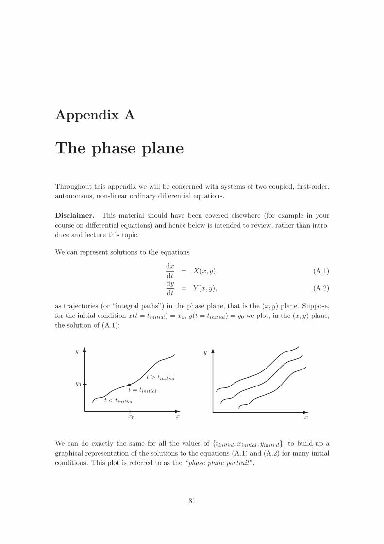
Appendix A
The phase plane
Throughout this appendix we will be concerned with systems of two coupled, first-order,
autonomous, non-linear ordinary differential equations.
Disclaimer. This material should have been covered elsewhere (for example in your
course on differential equations) and hence below is intended to review, rather than intro-
duce and lecture this topic.
We can represent solutions to the equations
dx
dt= X(x, y), (A.1)
dy
dt= Y (x, y), (A.2)
as trajectories (or “integral paths”) in the phase plane, that is the (x, y) plane. Suppose,
for the initial condition x(t = tinitial) = x0, y(t = tinitial) = y0 we plot, in the (x, y) plane,
the solution of (A.1):
We can do exactly the same for all the values of tinitial, xinitial, yinitial, to build-up a
graphical representation of the solutions to the equations (A.1) and (A.2) for many initial
conditions. This plot is referred to as the “phase plane portrait”.
81

Chapter A. The phase plane 82
A.1 Properties of the phase plane portrait
The gradient of the integral path through the point (x0, y0) is given by
dy
dx=
dy
dt
/dx
dt=
(Y (x, y)
X(x, y)
)∣∣∣∣(x0,y0)
=Y (x0, y0)
X(x0, y0). (A.3)
Key point 1. Note that if Y (x0, y0) = 0 and X(x0, y0) 6= 0 then
(dy
dx
)∣∣∣∣(x0,y0)
= 0, (A.4)
which corresponds to a horizontal line segments in the phase plane.
Key point 2. If Y (x0, y0) 6= 0 and X(x0, y0) = 0 then
∣∣∣∣
dy
dx
∣∣∣∣→ ∞ as (x, y) → (x0, y0), (A.5)
which corresponds to a vertical line segment in the phase plane.
Key point 3. Assuming that either X(x0, y0) 6= 0 or Y (x0, y0) 6= 0, then two path
integral curves do not cross at the point (x0, y0). This is because under these circumstances
dy/dx takes a unique value, i.e. the following is not possible:
A.2 Equilibrium points
Definition. A point in the phase plane where X(x0, y0) = Y (x0, y0) = 0 is defined
to be an equilibrium point, or equivalently, a stationary point.
The reason for the above definition is because if (x, y) = (x0, y0) then both dx/dt and
dy/dt are zero, and hence (x, y) do not change as t increases; hence x(t), y(t) remain at
(x0, y0) for all time.

Chapter A. The phase plane 83
Key point 1. Integral curves cannot cross at points which are not equilibrium points.
Key point 2. If an integral path ends it must end on a stationary point.
Key point 3. As we shall see below, equilibrium points are only approached as t→ ∞or t→ −∞.
However, what about the gradient of integral paths at (x0, y0)? We informally have
dy
dx=
0
0, (A.6)
which is not uniquely defined—the value ultimately depends on the details of how quickly
X(x, y) and Y (x, y) approach zero as (x, y) → (x0, y0), and this generally depends on the
direction upon which (x, y) approaches (x0, y0).
A.2.1 Equilibrium points: further properties
Suppose the equations (A.1) and (A.2) have an equilibrium point at (x0, y0). Thus
X(x0, y0) = Y (x0, y0) = 0. To determine the behaviour of integral paths close to the
equilibrium point we write
x = x0 + x, y = y0 + y, (A.7)
where it is assumed that x, y are sufficiently small to allow the approximations that we
will make below.
By Taylor expansion, we have
X(x, y) = X(x0 + x, y0 + y) = X(x0, y0) + x∂X
∂x(x0, y0) + y
∂X
∂y(x0, y0) + h.o.t.
= x∂X
∂x(x0, y0) + y
∂X
∂y(x0, y0) + h.o.t., (A.8)
using the fact X(x0, y0) = 0. Similarly, we have
Y (x, y) = Y (x0 + x, y0 + y) = Y (x0, y0) + x∂Y
∂x(x0, y0) + y
∂Y
∂y(x0, y0) + h.o.t.,
= x∂X
∂x(x0, y0) + y
∂X
∂y(x0, y0) + h.o.t. (A.9)
Note that x0 and y0 are constant, and hence have zero time derivative. Hence, by use
of Taylor expansions and neglecting higher orders (i.e. taking x, y sufficiently small), we
can neglect terms of the order O(xy, x2, y2
)and hence we can write equations (A.1) and
(A.2) in the form
du
dt=
(∂X∂x (x0, y0)
∂X∂y (x0, y0)
∂Y∂x (x0, y0)
∂Y∂y (x0, y0)
)
udef= Ju where u
def=
(
x
y
)
. (A.10)

Chapter A. The phase plane 84
Definition. The matrix
J =
(∂X∂x (x0, y0)
∂X∂y (x0, y0)
∂Y∂x (x0, y0)
∂Y∂y (x0, y0)
)
, (A.11)
is defined to be the Jacobian matrix at the equilibrium point (x0, y0).
A.3 Summary
The key points thus far are as follows.
1. We have taken the full non-linear equation system, (A.1) and (A.2), and expanded
about one of its (possibly many) equilibrium points taken to be located at (x0, y0),
using Taylor expansions of X(x, y), Y (x, y).
2. We assume that we are sufficiently close to (x0, y0) to enable us to only consider
linear terms of the order of (x− x0), (y − y0).
3. In this way, we obtain a set of two coupled, linear, autonomous ordinary differential
equations, i.e. equation (A.10) above, which in principle we can solve!
4. This procedure is sometimes referred to as “a linearisation of equations (A.1) and
(A.2) about the point (x0, y0)”.
5. In virtually all cases the behaviour of the linearised system is the same as the be-
haviour of the full non-linear equations sufficiently close to the point (x0, y0). In this
respect one should note that the statement immediately above can be formulated
more rigorously and proved for all the types of stationary points except:
• centre type equilibrium points, i.e. case [3c] below;
• the degenerate cases where λ1 = 0 and/or λ2 = 0, which are briefly mentioned in
item 2 on page (87). These stationary points can be considered non-examinable.
The relevant theorem is “Hartmann’s theorem”, as discussed further in P. Glendin-
ning, Stability, Instability and Chaos [4].
6. However, one should also note that the solution of the linearised equations may
behave substantially differently from the solutions of the full non-linear equations,
(A.1) and (A.2), sufficiently far from (x0, y0).
A.4 Investigating solutions of the linearised equations
We now have a set of two coupled, linear, autonomous ordinary differential equations,
(A.10). It is useful to look for a solution of the form
u = u0eλt, (A.12)
Chapter A. The phase plane 85
for some constant, λ. Substituting this into equation (A.10) we obtain
λu0eλt = Ju0e
λt i.e. (J − λI)u0 = 0. (A.13)
For a non-zero solution, we must have u0 6= (0, 0) and hence we require
det (J − λI) = 0, (A.14)
where I is the 2× 2 identity matrix.
This quadratic equation has two roots for λ, denoted λ1, λ2, which are possibly equal and
possibly complex; these are, of course, the eigenvalues of J evaluated at the point (x0, y0).
A.4.1 Case I
λ1, λ2 real, with λ1 6= 0, λ2 6= 0, λ1 6= λ2. Without loss of generality we take λ2 > λ1below.
We have two distinct, real eigenvalues. Let the corresponding eigenvectors be denoted by
e1 and e2. We thus have
Je1 = λ1e1, Je2 = λ2e2. (A.15)
We seek a solution of the form
u = A1e1 +A2e2. (A.16)
Substituting this into equation (A.10), we find, by comparing coefficients of e1 and e2,
thatdA1
dt= λ1A1,
dA2
dt= λ2A2, (A.17)
and hence
A1 = A1(t = 0)eλ1t, A2 = A2(t = 0)eλ2t. (A.18)
Thus we have (
x
y
)
def= u = A1(t = 0)eλ1te1 +A2(t = 0)eλ2te2, (A.19)
which gives us a representation of the solution of (A.10) for general initial conditions. This
information is best displayed graphically, and we do so below according to the values of
λ2, λ1.
Note. The equilibrium point i.e. (x, y) = (0, 0) can only be reached either as t→ ∞ or
t→ −∞.
1. λ1 < λ2 < 0. The phase plot of the linearised equations in the (x, y) plane looks
like one of the two possibilities in Figure A.1.
Definition. An equilibrium point which results in this case is called a stable
node, with the word “stable” referring to the fact that integral paths enter the
node, i.e. the equilibrium point at (0, 0).
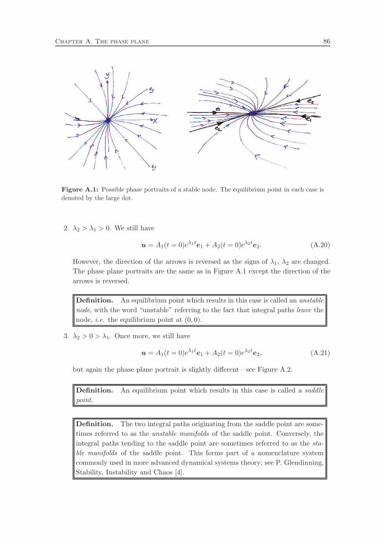
Chapter A. The phase plane 86
Figure A.1: Possible phase portraits of a stable node. The equilibrium point in each case is
denoted by the large dot.
2. λ2 > λ1 > 0. We still have
u = A1(t = 0)eλ1te1 +A2(t = 0)eλ2te2. (A.20)
However, the direction of the arrows is reversed as the signs of λ1, λ2 are changed.
The phase plane portraits are the same as in Figure A.1 except the direction of the
arrows is reversed.
Definition. An equilibrium point which results in this case is called an unstable
node, with the word “unstable” referring to the fact that integral paths leave the
node, i.e. the equilibrium point at (0, 0).
3. λ2 > 0 > λ1. Once more, we still have
u = A1(t = 0)eλ1te1 +A2(t = 0)eλ2te2, (A.21)
but again the phase plane portrait is slightly different—see Figure A.2.
Definition. An equilibrium point which results in this case is called a saddle
point.
Definition. The two integral paths originating from the saddle point are some-
times referred to as the unstable manifolds of the saddle point. Conversely, the
integral paths tending to the saddle point are sometimes referred to as the sta-
ble manifolds of the saddle point. This forms part of a nomenclature system
commonly used in more advanced dynamical systems theory; see P. Glendinning,
Stability, Instability and Chaos [4].

Chapter A. The phase plane 87
Figure A.2: The phase portrait of a saddle point. The equilibrium point is denoted by the
large dot.
A.4.2 Case II
λ2, λ1 real. One, or more, of the following also holds:
λ2 = λ1, λ1 = 0, λ2 = 0. (A.22)
We typically will not encounter these degenerate cases in this course. We briefly note
that behaviour of the full equations, (A.1), can be highly nontrivial when the linearisation
reduces to these degenerate cases. Further details of such cases can be found in P. Glendin-
ning, Stability, Instability and Chaos [4], which is on the reading list for this course. When
λ1, λ2 = 0, Hartmann’s theorem doesn’t hold.
A.4.3 Case III
λ2, λ1 complex. The complex eigenvalues of a real matrix always occur in complex conju-
gate pairs. Thus we take, without loss of generality,
λ1 = a− ib = λ∗2, λ2 = a+ ib = λ∗1, (A.23)
where a, b real, b 6= 0, and ∗ denotes the complex conjugate.
We also have two associated complex eigenvectors e1, e2, satisfying
Je1 = λ1e1, Je2 = λ2e2, (A.24)
which are complex conjugates of each other, i.e. e1 = e∗2.
Using the same idea as in Case I above, we have
u = A1(t = 0)eλ1te1 +A2(t = 0)eλ2te2, (A.25)
though now, in general, A1(t = 0), λ1, e1, A2(t = 0), λ2, e2 are complex, and hence so is
u.

Chapter A. The phase plane 88
Restricting u to be real gives
u = A1(t = 0)eλ1te1 +A∗1(t = 0)eλ2te2 = A1(t = 0)eλ1te1 + (A1(t = 0)eλ1te1)
∗, (A.26)
and this is real, as for any complex number z, we have z + z∗ ∈ R.
After some algebra this reduces to
u = eat [M cos(bt) +K sin(bt)] = eat
[(
M1
M2
)
cos(bt) +
(
K1
K2
)
sin(bt)
]
, (A.27)
whereM = (M1,M2)T , K = (K1,K2)
T are real, constant vectors, which can be expressed
in terms of A1(t = 0), A2(t = 0) and the components of the eigenvectors e1 and e2.
Equivalently, we have
x = eat [cos(bt)M1 + sin(bt)K1] , y = eat [cos(bt)M2 + sin(bt)K2] , (A.28)
where M1, M2, K1, K2 are real constants.
1. a > 0. We have x, y are, overall, increasing exponentially but are oscillating too.
For, example, with K1 = 0, M1 = 1 we have x = eat cos(bt), which looks like:
Note that the overall growth of x is exponential at rate a. Thus, in general, the
phase plane portrait looks like one of the examples shows in Figure A.3.
Note. The sense of the rotation, clockwise or anti-clockwise, is easily determined
by calculating dy/dt when y = 0 or dx/dt when x = 0.
Definition. An equilibrium point which results in the above, is called an un-
stable spiral or, equivalently, an unstable focus. The word “unstable” refers to
the fact that integral paths leave the equilibrium point.

Chapter A. The phase plane 89
Figure A.3: Possible phase portraits of a focus. The equilibrium point in each case is denoted
by the large dot.
2. a < 0. This is the same as 1. except now the phase plane portrait arrows point
towards the equilibrium point as x and y are exponentially decaying as time increases
rather than exponentially growing.
Definition. An equilibrium point which results in this case is called a stable
spiral or, equivalently, a stable focus. The word “stable” refers to the fact that
integral paths enter the equilibrium point.
3. a = 0. Thus we have λ2 = −ib = −λ1, b 6= 0, b real, and
x = [cos(bt)M1 + sin(bt)K1] , y = [cos(bt)M2 + sin(bt)K2] , (A.29)
where M1, M2, K1, K2 are constants. Note that
K2x−K1y = L cos(bt), −M2x+M1y = L sin(bt), (A.30)
where L = K2M1 − K1M2. Letting x∗ = K2x − K1y and y∗ = −M2x +M1y, we
have
(x∗)2 + (y∗)2 = L2, (A.31)
i.e. a circle in the (x∗, y∗) plane, enclosing the origin, which is equivalent to, in
general, a closed ellipse, in the (x, y) plane enclosing the origin.
Note. As with 3. above, the sense of the rotation, clockwise or anti-clockwise, is
easily determined by calculating dy/dt when y = 0 or dx/dt when x = 0.
Definition. An equilibrium point which results in this case, is called a centre.
A centre is an example of a limit cycle.

Chapter A. The phase plane 90
Definition. A limit cycle is an integral path which is closed (and which does not
have any equilibrium points).
A.5 Linear stability
Definition. An equilibrium point is linearly stable if the real parts of both eigenvalues
λ1, λ2 are negative.
From the expressions for u above, for example
u = A1(t = 0)eλ1te1 +A2(t = 0)eλ2te2, (A.32)
when λ1, λ2 real, we see that any perturbation away from the equilibrium decays back to
the equilibrium point.
Definition. An equilibrium point is linearly unstable if the real parts of at least one
of the eigenvalues λ1, λ2 is positive (and the other is non-zero).
Other situations are in general governed by the non-linear behaviour of the full equations
and we do not need to consider them here.
A.5.1 Technical point
The behaviour of the linearised equations and the behaviour of the non-linear equations
sufficiently close to the equilibrium point are guaranteed to be the same for any of the
equilibrium points [I 1-3], [III 1,2] or [II] with λ1 = λ2 6= 0. All these equilibrium points are
such that Re(λ1) Re(λ2) 6= 0. This is the essence of Hartmann’s theorem. This guarantee
does not hold for centres, or the equilibrium points described in [II] with λ1λ2 = 0.
The underlying reasons for this are as follows.
• First, note from the above that integral paths which meet the equilibrium point
can either grow/decay at exponential rate Re(λ1), or exponential rate Re(λ2), or
consist of the sum of two such terms. Second, note that in the above we took a
Taylor expansion. Including higher order terms in this Taylor expansion can lead to
a small correction for the rate of exponential decay towards or growth away from
the stationary point exhibited by the integral paths. These corrections tend to zero
as one approaches the equilibrium point.
• Consider the centre equilibrium point, which has Re(λ1) = Re(λ2) = 0, and an
exponential growth/decay of zero. If the corrections arising from the Taylor series are
always positive, the exponential growth/decay rate of all integral paths sufficiently
near the stationary point is always (slightly) positive. Hence these integral paths
grow exponentially away from the stationary point. However, b is non-zero, so x and
y are still oscillating. Hence one has the non-linear equations behave like a stable
focus.

Chapter A. The phase plane 91
• If Re(λ1), Re(λ2) 6= 0, then for all integral paths reaching the stationary point, the
above mentioned corrections, sufficiently close to the equilibrium point, are negligi-
ble, e.g. they cannot change exponential growth into exponential decay or vice-versa.
This allows one to show that stationary points with Re(λ1) Re(λ2) 6= 0 are guar-
anteed to have the same behaviour for the linearised and the non-linear equations
sufficiently close to the equilibrium point.
A.6 Summary
We will typically only encounter stationary points [I 1-3], [III 1-3]. Of these stationary
points, all but centres exhibit the same behaviour for the linearised and the non-linear
equations sufficiently close to the equilibrium point as plotted above and in D. W. Jordan
and P. Smith, Mathematical Techniques [6].

Bibliography
[1] N. F. Britton. Essential Mathematical Biology. Springer Undergraduate Mathematics
Series. Springer, 2005.
[2] L. Edelstein-Keshet. Mathematical Models in Biology. SIAM Classics in Applied
Mathematics, 2005.
[3] A. Gierer and H. Meinhardt. A theory of biological pattern formation. Kybernetik,
12:30–39, 1972.
[4] P. Glendinning. Stability, Instability and Chaos: An Introduction to the Theory of
Nonlinear Differential Equations. Cambridge Texts in Applied Mathematics, 1999.
[5] T. Hillen and K. Painter. A user’s guide to PDE models for chemotaxis. J. Math.
Biol., 58(1):183–217, 2009.
[6] D. W. Jordan and P. Smith. Mathematical Techniques: An Introduction for the En-
gineering, Physical and Mathematical Sciences. Oxford University Press, 3rd edition,
2002.
[7] J. P. Keener and J. Sneyd. Mathematical Physiology, volume 8 of Interdisciplinary
Applied Mathematics. Springer, New York, 1st edition, 1998.
[8] J. D. Murray. Mathematical Biology I: An Introduction, volume I. Springer-Verlag,
3rd edition, 2003.
[9] J. D. Murray. Mathematical Biology II: Spatial Models and Biochemical Applications,
volume II. Springer-Verlag, 3rd edition, 2003.
[10] A. Okubo, P. K. Maini, M. H. Williamson, and J. D. Murray. On the spread of the
grey squirrel in Great Britain. Proc. R. Soc. Lond. B, 238(1291):113–125, 1989.
[11] L. E. Reichl. A Modern Course in Statistical Physics. Wiley-VCH, 3rd edition, 2009.
[12] T. F. Weiss. Cellular Biophysics, volume 2. MIT Press, 1996.
92
Recommended

![Mathematical Models in Biology - Bio · PDF fileMathematical Models in Biology ... J.D., Mathematical Biology, Springer, 1989, [19] Edelstein-Keshet, Leah, Mathematical models in biology,](https://img.pdfslide.us/doc/110x75/5ab3fe3b7f8b9a7c5b8b587a/mathematical-models-in-biology-bio-models-in-biology-jd-mathematical-biology.jpg)