Master's Thesis in Structural Engineering
Material properties of concrete
used in skewed concrete
bridges
Author: Ahmed Saad
Surpervisor LNU: Johan Vessby
Examinar, LNU: Björn Johannesson
Course Code: 4BY35E
Semester: Spring 2016, 15 credits
Linnaeus University, Faculty of Technology

III
Abstract
This thesis has discussed both properties and geometry of concrete slabs used in
bridges.
It gave understanding on behavior of concrete in both tension and compression zones
and how crack propagates in specimens by presenting both theory of fracture and
performing concrete tests like tension splitting, uniaxial compression and uniaxial
tension tests.
Furthermore, it supported experimental tests with finite elements modelling for each
test, and illustrated both boundary conditions and loads.
The thesis has used ARAMIS cameras to observe crack propagations in all
experimental tests, and its first study at LNU that emphasized on Brazilian test,
because of importance of this test to describe both crushing and cracking behavior of
concrete under loading.
It’s an excellent opportunity to understand how concrete and steel behave
individually and in combination with each other, and to understand fracture process
zone, and this has been discussed in theory chapter.
The geometry change that could affect stresses distributions has also described in
literature and modelled to give good idea on how to model slabs in different angles in
the methodology chapter.
Thus, thesis will use finite elements program (Abaqus) to model both experimental
specimens and concrete slabs without reinforcement to emphasize on concrete
behavior and skewness effect. This means studying both properties of concrete and
geometry of concrete slabs. This thesis has expanded experimental tests and chose
bridges as an application.
Key words: crack, skew slab, RCC slabs, fracture process zone, uniaxial
compression test, uniaxial tension test, Brazilian splitting tension test, modelling
linear behavior of concrete, bridges.

IV
Acknowledgement
This thesis is for a degree of Master of Science in structural engineering program at
the department of Building technology at Linnaeus University.
My great thanks and appreciation to all those who supported me and helped me to
success in this thesis and program, to mention my supervisor Professor Johan Vessby
and our laboratory supervisor Mr. Bertil Enquit.
My great thanks as well to my colleagues in the department of Building engineering
who were nice and helpful.
Ahmed Saad
Växjö 25th of May 2016
V
Table of Notations and Abbreviations
Symbol Definition
𝑓𝑐𝑡𝑚 Mean concrete tensile strength(28 days) [MPa]
𝑓𝑐𝑐𝑚 Mean concrete compressive strength (28 days) [MPa]
𝑓𝑓𝑡𝑚 Mean flexural strength [MPa]
Ecsm Secant modulus of elasticitiy [GPa]
Ec𝑦𝑚 Young’s modulus of elascticity [GPa]
ε Strain, difference in shape of elongation or shrinkage
divided by undeformerd total length , unitless
𝐾𝐼𝑐 Fracture toughness [N/m]
𝑓′ Mean concrete compressive strength (28 days) [MPa]
𝐺𝑐 Fractute energy [J/ 𝑚2]
lcℎ Chateristic fracture zone process length[mm]
l𝑝 Fracture zone process length [mm]
𝑓𝑏𝑘 is tensile strength for splitting tension test based on
(Brazilian test) in [MPa]
𝑓𝑐𝑡 tensile strength of direct tension test in MPa, 𝑓𝑏 is tensile
strength for splitting tension test (brazilian test) [MPa]
∝F Unitless coffiecent depends on aggregate maximum size
𝑓𝑏𝑘 is characteristic tensile strength for splitting tension test
(Brazilian test) [MPa],
𝑓𝑐𝑘 is characteristic concrete compressive strength in [Mpa]
fctk characteristic direct tensile strength [MPa] (Olukun)
𝐸′ Young’s modulus of elasticity [GPa]
VI
Table of contents
1. INTRODUCTION.......................................................................................................... 1
1.1 BACKGROUND ................................................................................................................................... 2 1.2 AIM AND PURPOSE ................................................................................................................................ 7 1.3 HYPOTHESIS AND LIMITATIONS ............................................................................................................. 7 1.4 RELIABILITY, VALIDITY AND OBJECTIVITY ............................................................................................ 7
2. LITERATURE REVIEW ............................................................................................. 8
2.1. EFFECT OF INCREASE IN THE SKEW ANGLE IN STATIC BEHAVIOR FOR BRIDGES ..................................... 8 2.1.1 Deflection...................................................................................................................................... 8 2.1.2 Crack and ultimate load ............................................................................................................... 9
2.2 RCC SLABS BEHAVIOR AND THEIR MATERIAL PROPERTIES. ................................................................... 9
3. THEORY ...................................................................................................................... 11
3.1 CONCRETE MATERIAL.......................................................................................................................... 11 3.2 STEEL MATERIAL ................................................................................................................................. 14 3.3 REINFORCED CEMENTOUS CONCRETE (RCC) BEHAVIOR .................................................................... 14 3.4 CRACK GROWTH ON CONCRETE SUBJECTED TO TENSION ..................................................................... 15 3.5 CRACKS IN RCC SLABS AND CONCRETE .............................................................................................. 18
3.5.1 Concrete material matrix ............................................................................................................ 18 3.5.2 Fracture mechanics theory and equations .................................................................................. 19 3.5.3 Empirical relation between strength parameters in concrete ..................................................... 21 3.5.4 Equations for evaluation of experimental test ............................................................................ 23 3.5.5 Stresses in Brazilian test ............................................................................................................. 24
4. METHOD ..................................................................................................................... 26
4.1 EXPERIMENTAL TESTS ......................................................................................................................... 26 4.1.1 Brazilian splitting tension (brazilin test) .................................................................................... 27 4.1.2 Uniaxial compression test ........................................................................................................... 27 4.1.3 Direct uniaxial tension test ......................................................................................................... 28
4.2 FINITE ELEMENT MODELLING (FEM) ................................................................................................... 29 4.2.1 Linear behavior of concrete in FEM .......................................................................................... 29
4.3 ANALYTICAL METHOD ......................................................................................................................... 30 4.4 STRESSES AT CORNERS OF SLABS WITH GEOMETRY CHANGE ............................................................... 30
5. RESULTS ..................................................................................................................... 31
5.1 EXPERIMENTAL AND CRACK PROPAGATIONS RESULTS ........................................................................ 31 5.1.1 Brazilian splitting tension test .................................................................................................... 31 5.1.2 Uniaxial compression test ........................................................................................................... 34 5.1.3 Direct uniaxial Tension Test ....................................................................................................... 37 5.1.4 Overall observed data for experimental tests ............................................................................. 41
5.2 FEM MODELLING RESULLTS .............................................................................................................. 41 5.2.1 Brazilian Splitting Tension Test modelling ................................................................................. 41 5.2.2 Uniaxial compression test modelling .......................................................................................... 43 5.2.3 Direct uniaxial tension Test modelling ...................................................................................... 46 5.2.4 Stresses modelling in slabs ......................................................................................................... 47
6. ANALYSIS ................................................................................................................... 49
6.1 BRAZILIAN SPLITTING TEST ................................................................................................................. 49 6.2 UNIAXIAL COMPRESSION TEST ............................................................................................................ 51 6.3 DIRECT UNIAXIAL TENSION TEST ......................................................................................................... 53 6.4 STRESSES IN CONCRETE SLABS WITH GEOMETRY CHANGE ................................................................... 53
7. DISCUSSION ............................................................................................................... 55

VII
8. CONCLUSION ............................................................................................................ 56
9. FUTURE WORK ......................................................................................................... 57
9.1.1 The smeared crack concrete model............................................................................................. 57 9.1.2 Concrete damage plasticity ........................................................................................................ 57
REFERENCES ................................................................................................................. 59
APPENDIXES .................................................................................................................. 61
1
Ahmed Saad
1. Introduction
Nowadays, it’s important to have reliable infrastructure that could withstand
the human needs, this infrastructure is important in any country, however
infrastructure examples could be found as roads, bridges, tunnels, dams, etc.
The bridge is one of important structural elements in our infrastructure,
however, first bridge found was Arkadiko bridge in Greece which is oldest
arch bridges in the world, it has been built back to 13th century BC, and
Danyang–Kunshan grand bridge in China, is one of longest bridges in the
world, with total distance of 165 km.
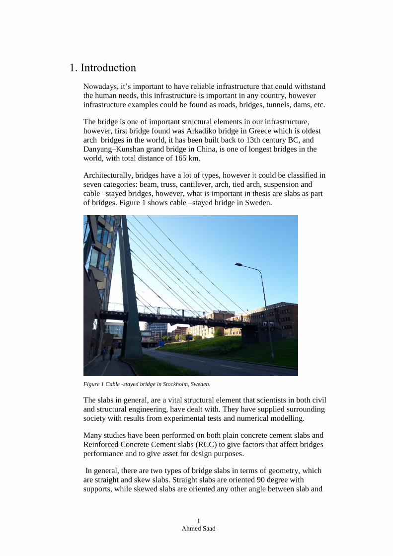
Architecturally, bridges have a lot of types, however it could be classified in
seven categories: beam, truss, cantilever, arch, tied arch, suspension and
cable –stayed bridges, however, what is important in thesis are slabs as part
of bridges. Figure 1 shows cable –stayed bridge in Sweden.
Figure 1 Cable -stayed bridge in Stockholm, Sweden.
The slabs in general, are a vital structural element that scientists in both civil
and structural engineering, have dealt with. They have supplied surrounding
society with results from experimental tests and numerical modelling.
Many studies have been performed on both plain concrete cement slabs and
Reinforced Concrete Cement slabs (RCC) to give factors that affect bridges
performance and to give asset for design purposes.
In general, there are two types of bridge slabs in terms of geometry, which
are straight and skew slabs. Straight slabs are oriented 90 degree with
supports, while skewed slabs are oriented any other angle between slab and

2
Ahmed Saad
supports. Skew slabs are the most common in practice because they fit the
best to the landscape.
A lot of studies have been performed for these two types of slabs, especially
the skew ones, including loadings in different positions of slabs, modellings
that includes both grillage and finite element method (FEM), grillage
method is much practical and easy using stiffness matrices and degree of
skewness for bridge slabs.
Furthermore, both static, dynamic and material analysis have been taken in
many tests all over the world, to give us good idea about environmental
impacts, stresses, and strains, and even vibrations, all that to study the
behavior of these slabs.
However, this thesis will use finite elements program (Abaqus) to model
both experimental specimens and concrete slabs without reinforcement to
emphasize on concrete behavior and skewness effect.This means studying
both properties of concrete and geometry of concrete slabs. This thesis has
expanded experimental tests and chose bridges as an application.
1.1 Background
Skew slabs are very popular due its geometry flexibility to obstructions in
real sites.
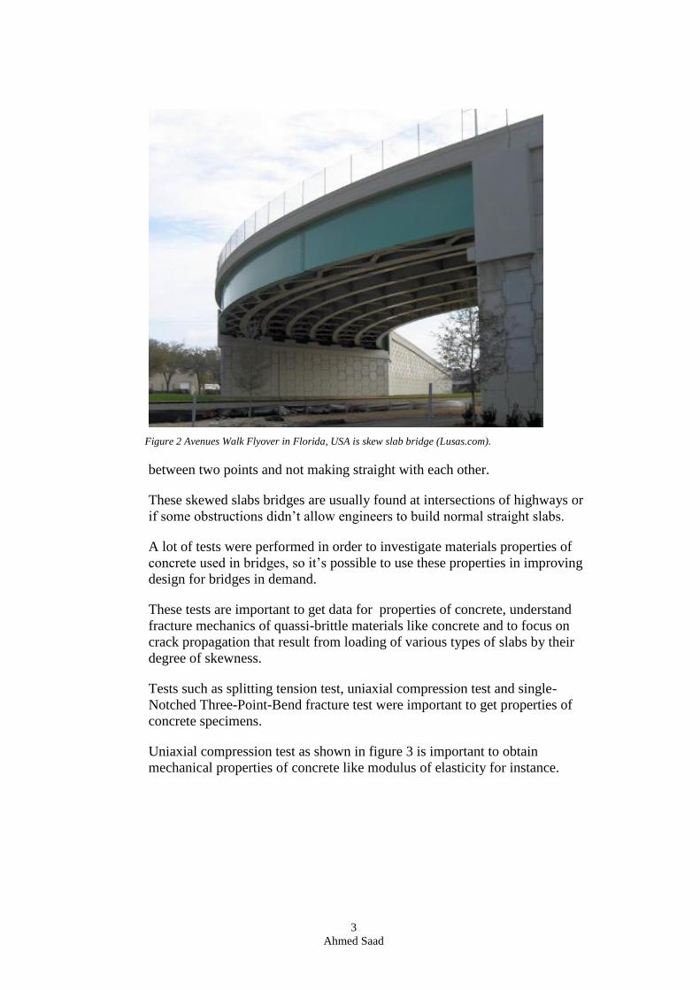
The increasing of population will require building more roads and highways,
and this will result that more intersections will be built, as seen in figure 2,
that shows typical skew slab bridge that connect road
3
Ahmed Saad
Figure 2 Avenues Walk Flyover in Florida, USA is skew slab bridge (Lusas.com).
between two points and not making straight with each other.
These skewed slabs bridges are usually found at intersections of highways or
if some obstructions didn’t allow engineers to build normal straight slabs.
A lot of tests were performed in order to investigate materials properties of
concrete used in bridges, so it’s possible to use these properties in improving
design for bridges in demand.
These tests are important to get data for properties of concrete, understand
fracture mechanics of quassi-brittle materials like concrete and to focus on
crack propagation that result from loading of various types of slabs by their
degree of skewness.
Tests such as splitting tension test, uniaxial compression test and single-
Notched Three-Point-Bend fracture test were important to get properties of
concrete specimens.
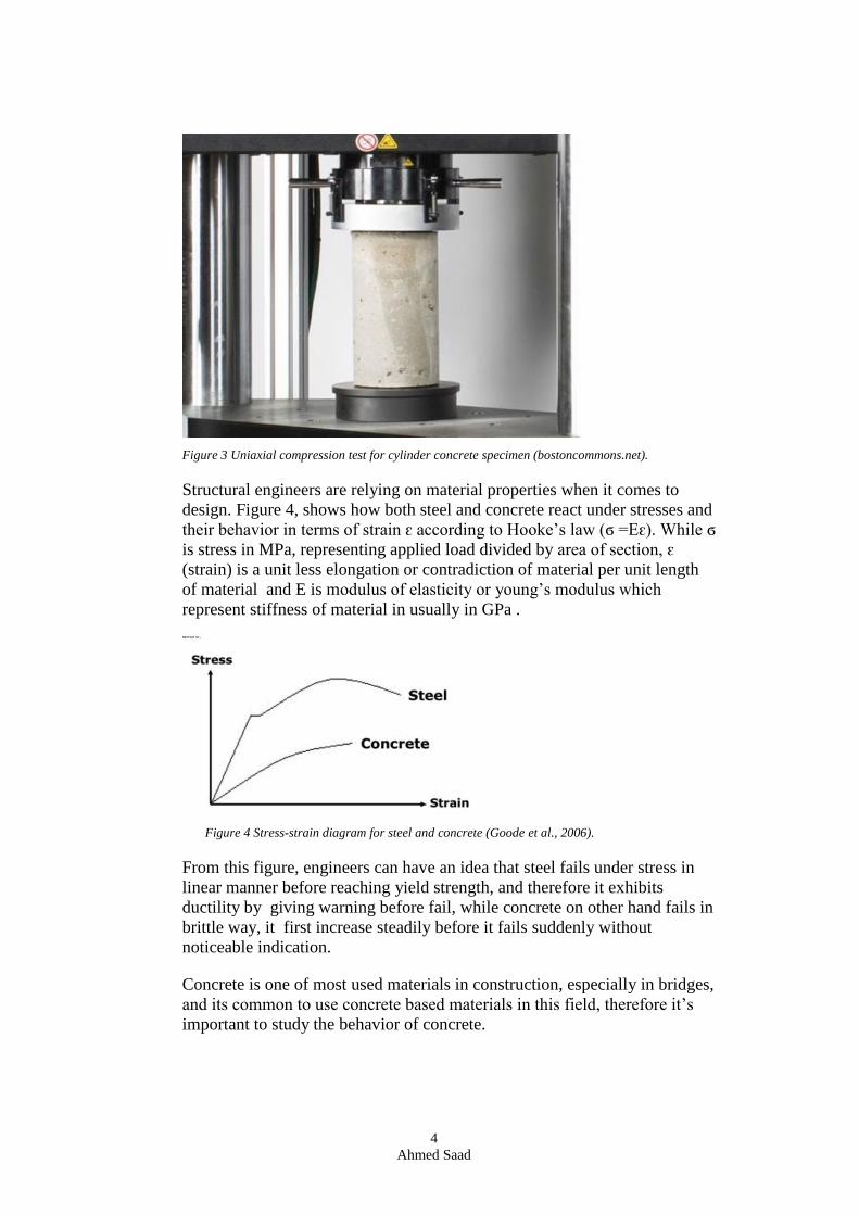
Uniaxial compression test as shown in figure 3 is important to obtain
mechanical properties of concrete like modulus of elasticity for instance.
4
Ahmed Saad
Figure 3 Uniaxial compression test for cylinder concrete specimen (bostoncommons.net).
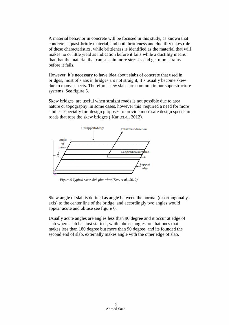
Structural engineers are relying on material properties when it comes to
design. Figure 4, shows how both steel and concrete react under stresses and
their behavior in terms of strain ԑ according to Hooke’s law (ϭ =Eԑ). While ϭ
is stress in MPa, representing applied load divided by area of section, ԑ
(strain) is a unit less elongation or contradiction of material per unit length
of material and E is modulus of elasticity or young’s modulus which
represent stiffness of material in usually in GPa .
Figure 4 Stress-strain diagram for steel and concrete (Goode et al., 2006).
From this figure, engineers can have an idea that steel fails under stress in
linear manner before reaching yield strength, and therefore it exhibits
ductility by giving warning before fail, while concrete on other hand fails in
brittle way, it first increase steadily before it fails suddenly without
noticeable indication.
Concrete is one of most used materials in construction, especially in bridges,
and its common to use concrete based materials in this field, therefore it’s
important to study the behavior of concrete.
5
Ahmed Saad
A material behavior in concrete will be focused in this study, as known that
concrete is quasi-brittle material, and both brittleness and ductility takes role
of these characteristics, while brittleness is identified as the material that will
makes no or little yield as indication before it fails while a ductility means
that that the material that can sustain more stresses and get more strains
before it fails.
However, it’s necessary to have idea about slabs of concrete that used in
bridges, most of slabs in bridges are not straight, it’s usually become skew
due to many aspects. Therefore skew slabs are common in our superstructure
systems. See figure 5.
Skew bridges are useful when straight roads is not possible due to area
nature or topography ,in some cases, however this required a need for more
studies especially for design purposes to provide more safe design speeds in
roads that tops the skew bridges ( Kar ,et.al, 2012).
Figure 5 Typical skew slab plan view (Kar, et al., 2012).
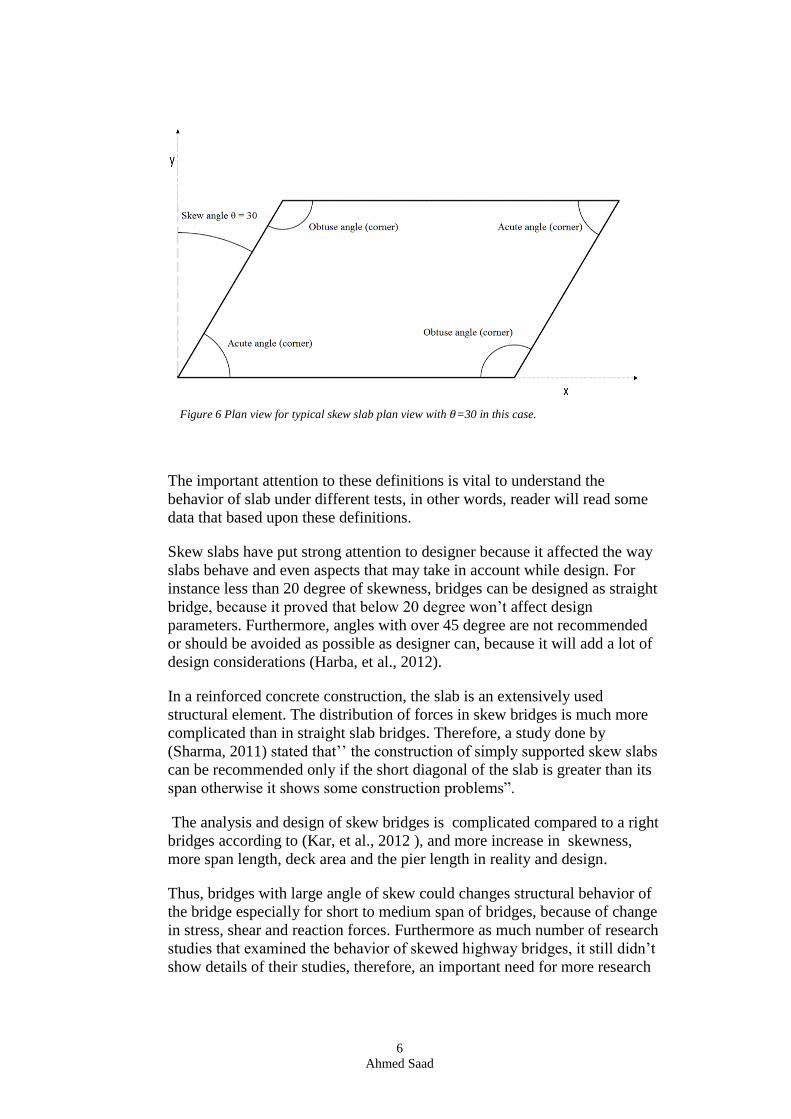
Skew angle of slab is defined as angle between the normal (or orthogonal y-
axis) to the center line of the bridge, and accordingly two angles would
appear acute and obtuse see figure 6.
Usually acute angles are angles less than 90 degree and it occur at edge of
slab where slab has just started , while obtuse angles are that ones that
makes less than 180 degree but more than 90 degree and its founded the
second end of slab, externally makes angle with the other edge of slab.
6
Ahmed Saad
Figure 6 Plan view for typical skew slab plan view with 𝜃=30 in this case.
The important attention to these definitions is vital to understand the
behavior of slab under different tests, in other words, reader will read some
data that based upon these definitions.
Skew slabs have put strong attention to designer because it affected the way
slabs behave and even aspects that may take in account while design. For
instance less than 20 degree of skewness, bridges can be designed as straight
bridge, because it proved that below 20 degree won’t affect design
parameters. Furthermore, angles with over 45 degree are not recommended
or should be avoided as possible as designer can, because it will add a lot of
design considerations (Harba, et al., 2012).
In a reinforced concrete construction, the slab is an extensively used
structural element. The distribution of forces in skew bridges is much more
complicated than in straight slab bridges. Therefore, a study done by
(Sharma, 2011) stated that’’ the construction of simply supported skew slabs
can be recommended only if the short diagonal of the slab is greater than its
span otherwise it shows some construction problems”.
The analysis and design of skew bridges is complicated compared to a right
bridges according to (Kar, et al., 2012 ), and more increase in skewness,
more span length, deck area and the pier length in reality and design.
Thus, bridges with large angle of skew could changes structural behavior of
the bridge especially for short to medium span of bridges, because of change
in stress, shear and reaction forces. Furthermore as much number of research
studies that examined the behavior of skewed highway bridges, it still didn’t
show details of their studies, therefore, an important need for more research
7
Ahmed Saad
to study the effect of skew angle on the performance of highway bridges is
significantly required.
While skewed bridges are increasingly popular in roads and highways, many
questions need additional research for better understanding to their
performance and to provide additional scientific grounds for super structural
design for more safe, comfortable and economic bridges.
1.2 Aim and Purpose
The aim of this study is to analyze the material properties for straight and
skew concrete based slabs, and to investigate failure behavior, stress
concentration in different positions of materials.
To accomplish this both compression and tension tests will be processed for
the specimens to figure out behavior phenomenon such as cracks.
The purpose is to understand properties of materials used in bridges, and to
analyze larger elements like skewed bridges to be able to capture stresses
concentrations and cracking in those types.
1.3 Hypothesis and Limitations
The hypothesis for this study is to focus on behavior of tension capacity of
concrete that is usually used in bridges. The work is limited to certain test
conditions, class of concrete and specimens performed at laboratory of LNU,
and are frequently used in bridges.
Furthermore, only finite element software Abaqus will be used for the
analysis, and linear elastic material properties will be used, and
reinforcement bars will not be included in the analysis.
1.4 Reliability, validity and objectivity
The study is based on some experimental data from laboratory tests in
Linnaeus University, and the validity of the data will be based on design
mix that follows standards according to EC, however, design mix that given
by supplier and laboratory conditions during experiments are factors that
were very hard to control them.
8
Ahmed Saad
2. Literature Review
In this section, there will be an illustration of previous studies and
importance of studying the effect of both material and geometry of RCC
bridges.
As known that as many non-straight slabs in bridges caused a need for the
study of behavior for RCC slabs due to skewness which has begun many
years ago.
For instance, early studies have utilized the least work method to analyze
stresses in slabs. Later ,The design of skewed concrete slab bridges using the
equivalent-beam method (Massicotte, et al., 2012) is described in scientific
paper, through calculating bending moment and shear forces in first stage
according to research by (Pandey, et al., 2014), however, scientists have
studied both static and dynamic factors affecting bridges, reader can get
more information by reading dynamic effects like what (Bisadi, et al., 2013)
have wrote and other researchers, which is not introduced in this study.
This study will take misses stresses on corners of non-reinforced concrete
slabs and other factors are not included.
2.1. Effect of increase in the skew angle in static behavior for bridges
A study by (kar, et al., 2012), has discussed that when the skew angle
increased, the stresses in terms of magnitude and distribution will be
different from those in a straight slab.
Furthermore, a lot of study cases has been performed to analyze this effect,
for instance applied loads transfer has a direct proportion with rigidity of
paths this load will take, even a lot of studies about skewness effect on
reactions, moments, shear, deflections and cracks have been discussed with
both (Sindhu B.V.et al, 2013) and (Miah, et al., 2005).
However this study is discussing only deflection and cracks phenomena in
this section, and only misses stresses on corners of non-reinforced linear
slabs will be obtained by modelling program (Abaqus) in the method
section.
2.1.1 Deflection
A study by (Miah, et al., 2005) has proved that the maximum deflection that
occur for skewed slab regardless loading types (whether point or
concentrated load) has noticed to be more when degree of skewness has
increased.
9
Ahmed Saad
Furthermore, a study done by (Sindhu, et al., 2013) has showed a lot of
experimental data analysis to study the effect of skewness on deflection and
other factors, reader can see this interesting study by looking through
reference.
2.1.2 Crack and ultimate load
Same study done by (Miah, et al., 2005) showed that ultimate load when the
crack happen was less when degree of skewness has increased.
Ultimate load is defined as load that applied to slabs until they collapse, so
it has been proved that due to skewness effect, slabs are no longer capable to
sustain same loads as straight slabs.
This effect has been investigated by scientists by applying both distributed
and point loads to slabs in different degree of skewness according to (Bisadi,
et al., 2013).
2.2 RCC slabs behavior and their material properties.
Reinforced concrete slabs are structural materials that became very popular
in construction, however these elements work in both ductile and brittle
manner, this attitude has encouraged scientists to identify many ways to
study this behavior using both experimental and finite element modelling to
figure out how it works.
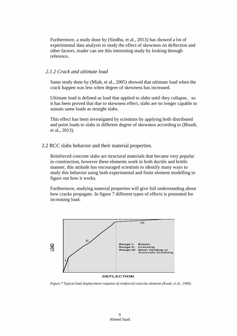
Furthermore, studying material properties will give full understanding about
how cracks propagate. In figure 7 different types of effects is presented for
increasing load.
Figure 7 Typical load displacement response of reinforced concrete elements (Kwak, et al., 1990).
10
Ahmed Saad
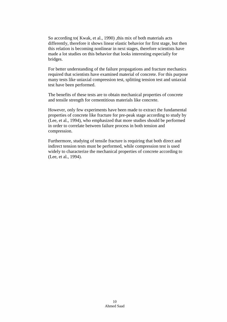
So according to( Kwak, et al., 1990) ,this mix of both materials acts
differently, therefore it shows linear elastic behavior for first stage, but then
this relation is becoming nonlinear in next stages, therefore scientists have
made a lot studies on this behavior that looks interesting especially for
bridges.
For better understanding of the failure propagations and fracture mechanics
required that scientists have examined material of concrete. For this purpose
many tests like uniaxial compression test, splitting tension test and uniaxial
test have been performed.
The benefits of these tests are to obtain mechanical properties of concrete
and tensile strength for cementitious materials like concrete.
However, only few experiments have been made to extract the fundamental
properties of concrete like fracture for pre-peak stage according to study by
(Lee, et al., 1994), who emphasized that more studies should be performed
in order to correlate between failure process in both tension and
compression.
Furthermore, studying of tensile fracture is requiring that both direct and
indirect tension tests must be performed, while compression test is used
widely to characterize the mechanical properties of concrete according to
(Lee, et al., 1994).
11
Ahmed Saad
3. Theory
In the two previous chapters, many scientific terms have been identified,
giving the reader background about bridges in terms of both geometry and
material.
Hence there is a need for understanding material properties, and how crack
propagate depending on concrete properties.
Therefore, understanding properties is very important to understand crack
propagation and stress concentration in real RCC slabs in bridges.
3.1 Concrete material
RCC slabs have two major components, steel and concrete. Concrete as
main component of slabs is giving a very good idea about how this mixture
would affect the behavior of slabs in both tension and compression.
Concrete is a quasi-brittle material which is different than steel that act as
elastic-plastic or even ductile material.
Concrete is a material that has a compromised mixture of different types of
materials, and that is why its referred to as a heterogeneous material, it
contains water, cement, sand, coarse aggregate, and these components have
a design mix that vary from design mix to another depending on the required
compressive strength that should be met.
This strength is measured after 28 days which is different between cylinder
and cube specimens, for instance C30/37 means that characteristic
compressive strength 𝑓𝑐𝑘 =30 MPa for cylinder and 37 MPa for cube,
according to Eurocode 2 and EN 206-1, according to (Banforth, 2000).
However, mean compressive strength for C30/37 after 28 days, for both
cylinder and cube are 38 and 47 MPa accordingly.
Concrete has a lot of classes and table 1 has illustrated the most used classes
according to Euro code 2
12
Ahmed Saad
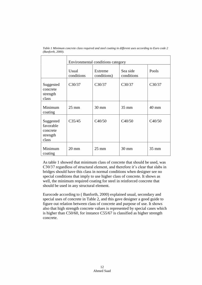
Table 1 Minimum concrete class required and steel coating in different uses according to Euro code 2
(Banforth, 2000).
Environmental conditions category
Usual
conditions
Extreme
conditions)
Sea side
conditions
Pools
Suggested
concrete
strength
class
C30/37 C30/37 C30/37 C30/37
Minimum
coating
25 mm 30 mm 35 mm 40 mm
Suggested
favorable
concrete
strength
class
C35/45 C40/50 C40/50 C40/50
Minimum
coating
20 mm 25 mm 30 mm 35 mm
As table 1 showed that minimum class of concrete that should be used, was
C30/37 regardless of structural element, and therefore it’s clear that slabs in
bridges should have this class in normal conditions when designer see no
special conditions that imply to use higher class of concrete. It shows as
well, the minimum required coating for steel in reinforced concrete that
should be used in any structural element.
Eurocode according to ( Banforth, 2000) explained usual, secondary and
special uses of concrete in Table 2, and this gave designer a good guide to
figure out relation between class of concrete and purpose of use. It shows
also that high strength concrete values is represented by special cases which
is higher than C50/60, for instance C55/67 is classified as higher strength
concrete.
13
Ahmed Saad
Table 2 Relation between purpose of use and class of concrete according to Euro code 2 (Banforth, 2000).
Usual uses C30/37 C35/45 C40/50 C45/55 C50/60
Secondary
uses
C12/15 C16/20 C20/25 C25/30 -----------
Special
uses
C55/67 C60/75 C70/85 C80/95 C90/105
Concrete has a very sensitive characteristics, for instance it has two major
characteristic measures, compression and tension strengths.
These two strengths acting in a way different than another, for instance its
tension strength is approximately one tenth its compression strength.
Therefore its capable or maximum tension is very important for design of
bridges or where else structural element, (Karihaloo, 2001).
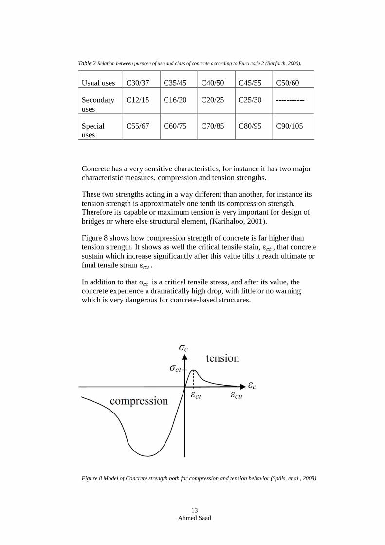
Figure 8 shows how compression strength of concrete is far higher than
tension strength. It shows as well the critical tensile stain, ԑ𝑐𝑡 , that concrete
sustain which increase significantly after this value tills it reach ultimate or
final tensile strain ԑ𝑐𝑢 .
In addition to that ϭ𝑐𝑡 is a critical tensile stress, and after its value, the
concrete experience a dramatically high drop, with little or no warning
which is very dangerous for concrete-based structures.
Figure 8 Model of Concrete strength both for compression and tension behavior (Spåls, et al., 2008).
14
Ahmed Saad
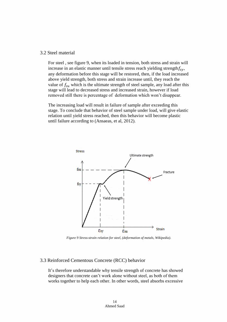
3.2 Steel material
For steel , see figure 9, when its loaded in tension, both stress and strain will
increase in an elastic manner until tensile stress reach yielding strength𝑓𝑠𝑦,
any deformation before this stage will be restored, then, if the load increased
above yield strength, both stress and strain increase until, they reach the
value of 𝑓𝑠𝑢 which is the ultimate strength of steel sample, any load after this
stage will lead to decreased stress and increased strain, however if load
removed still there is percentage of deformation which won’t disappear.
The increasing load will result in failure of sample after exceeding this
stage. To conclude that behavior of steel sample under load, will give elastic
relation until yield stress reached, then this behavior will become plastic
until failure according to (Ansaeas, et al, 2012).
Figure 9 Stress-strain relation for steel, (deformation of metals, Wikipedia).
3.3 Reinforced Cementous Concrete (RCC) behavior
It’s therefore understandable why tensile strength of concrete has showed
designers that concrete can’t work alone without steel, as both of them
works together to help each other. In other words, steel absorbs excessive
15
Ahmed Saad
tension stresses that concrete couldn’t withstand, and concrete protect steel
from buckling when reinforced concrete slabs experience compression
stresses.
Thus, in general, in reinforced concrete slabs, both steel and concrete works
in a linear relation until stresses reaches tensile strength of concrete which is
the weaker in this case.
Thereafter, the relation become non-linear and crack starts to propagate in
concrete (because concrete has weak tensile strength) in the next stage.
However, the value of when sample at second stage fails is not easy to be
predicted due to the fact that rest of sample stiffness try to minimize or slow
down crack propagation, and this phenomena is called tension stiffening
effect according to (Spåls et al., 2008).
Its therefore became an important to know what’s actually happen for both
concrete and steel when loading takes place.
3.4 Crack growth on concrete subjected to tension
Concrete behavior has encouraged scientists to study the behavior of
concrete under both compression and tension, and they concluded that
concrete behave in gradual drop after reaching its compressive strength, and
therefore it fails when exceeding its stress softening stage.
Tensile strength for concrete, on other hand, is much less than its
compressive strength and it fails in sudden manner, when it’s exceeding the
stage of strain softening (Deb, 2000).
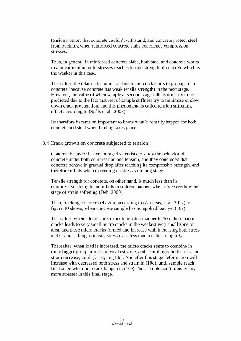
Then, tracking concrete behavior, according to (Ansaeas, et al, 2012) as
figure 10 shows, when concrete sample has no applied load yet (10a).
Thereafter, when a load starts to act in tension manner in 10b, then macro
cracks leads to very small micro cracks in the weakest very small zone or
area, and these micro cracks formed and increase with increasing both stress
and strain, as long as tensile stress ϭ𝑡 is less than tensile strength 𝑓𝑡 .
Thereafter, when load is increased, the micro cracks starts to combine in
more bigger group or mass in weakest zone, and accordingly both stress and
strain increase, until 𝑓𝑡 =ϭ𝑡 in (10c). And after this stage deformation will
increase with decreased both stress and strain in (10d), until sample reach
final stage when full crack happen in (10e).Thus sample can’t transfer any
more stresses in this final stage.
16
Ahmed Saad
Figure 10 Concrete specimen in tension with cases (a) no load and sample is perfect (b) stress less
than tension strength (c) stress equal to tensile strength (d) stress exceeded tensile stress (e) no more
stresses for completely cracked specimen (Ansnaes, et al., 2012)
Hence, scientists have classified all possible ways that crack could propagate
which are opening, sliding and tearing modes, according to (Karihaloo,
2001).
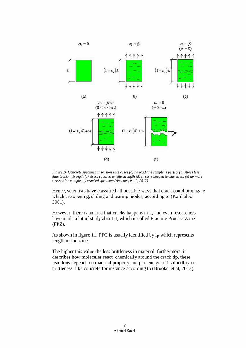
However, there is an area that cracks happens in it, and even researchers
have made a lot of study about it, which is called Fracture Process Zone
(FPZ).
As shown in figure 11, FPC is usually identified by lP which represents
length of the zone.
The higher this value the less brittleness in material, furthermore, it
describes how molecules react chemically around the crack tip, these
reactions depends on material property and percentage of its ductility or
brittleness, like concrete for instance according to (Brooks, et al, 2013).
17
Ahmed Saad
Figure 11 Fracture process zone is occurring in (BCD) zone (Karihaloo, 2001).
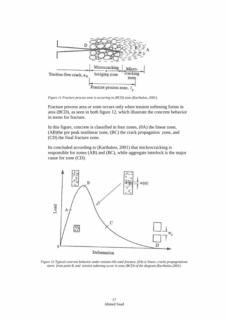
Fracture process area or zone occurs only when tension softening forms in
area (BCD), as seen in both figure 12, which illustrate the concrete behavior
in terms for fracture.
In this figure, concrete is classified in four zones, (0A) the linear zone,
(AB)the pre peak nonlinear zone, (BC) the crack propagation zone, and
(CD) the final fracture zone.
Its concluded according to (Karihaloo, 2001) that mickrocracking is
responsible for zones (AB) and (BC), while aggregate interlock is the major
cause for zone (CD).
Figure 12 Typical concrete behavior under tension tills total fracture, (0A) is linear, cracks propagrtations
starts from point B, and tension softening occur in zone (BCD) of the diagram (Karihaloo,2001).
18
Ahmed Saad
3.5 Cracks in RCC slabs and concrete
Concrete and steel behave in different ways when load is applied, while steel
act as ductile due to yielding and in almost linear manner, concrete, behaves,
in nonlinear relation between stress and strain, when subjected for large
tensional forces.
Cracks will develop due tension stresses, and, scientists have studied cracks
in many ways.
Cracks in concrete have many reasons, and they are classified into two
major classes: before-hardening and after- hardening.
There are many sub classes under both categories, however this study is
discussing only after-hardening cracks with reason of applied mechanical
loading (Kelly, 1964)
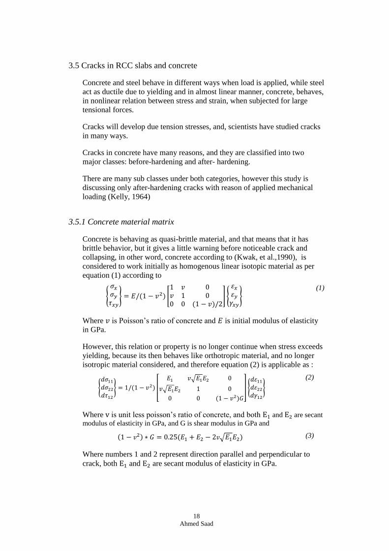
3.5.1 Concrete material matrix
Concrete is behaving as quasi-brittle material, and that means that it has
brittle behavior, but it gives a little warning before noticeable crack and
collapsing, in other word, concrete according to (Kwak, et al.,1990), is
considered to work initially as homogenous linear isotopic material as per
equation (1) according to
{
𝜎𝑥
𝜎𝑦
𝜏𝑥𝑦
} = 𝐸/(1 − 𝑣2) [1 𝑣 0𝑣 1 00 0 (1 − 𝑣)/2
] {
𝜀𝑥
𝜀𝑦
𝛾𝑥𝑦
} (1)
Where 𝑣 is Poisson’s ratio of concrete and 𝐸 is initial modulus of elasticity
in GPa.
However, this relation or property is no longer continue when stress exceeds
yielding, because its then behaves like orthotropic material, and no longer
isotropic material considered, and therefore equation (2) is applicable as :
{
𝑑𝜎11
𝑑𝜎22
𝑑𝜏12
} = 1/(1 − 𝑣2) [
𝐸1 𝑣√𝐸1𝐸2 0
𝑣√𝐸1𝐸2 1 0
0 0 (1 − 𝑣2)𝐺
] {
𝑑𝜀11
𝑑𝜀22
𝑑𝛾12
}
(2)
Where v is unit less poisson’s ratio of concrete, and both E1 and E2 are secant
modulus of elasticity in GPa, and G is shear modulus in GPa and
(1 − 𝑣2) ∗ 𝐺 = 0.25(𝐸1 + 𝐸2 − 2𝑣√𝐸1𝐸2) (3)
Where numbers 1 and 2 represent direction parallel and perpendicular to
crack, both E1 and E2 are secant modulus of elasticity in GPa.
19
Ahmed Saad
There are more equations to represent proper matrix for concrete when
cracks from loads occurred, and reader can read more from (Kwak, 1990).
3.5.2 Fracture mechanics theory and equations
Scientists have investigated crack in many aspects, for instance through
studying its physical and mechanical behavior on infinitesimal references,
and they identified both modes in which crack occur, as well as crack
fracture zone, and they concluded that crack happen in three modes :
opening ,sliding and tearing modes (Karihaloo,2001).
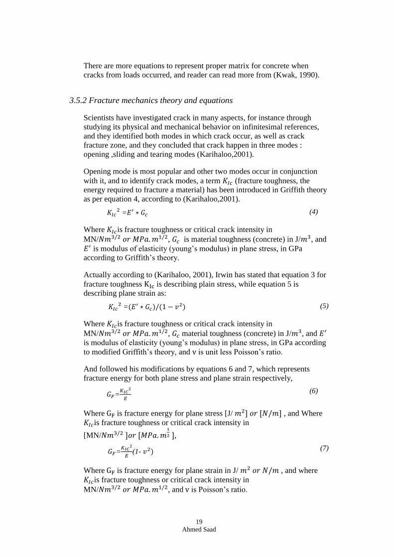
Opening mode is most popular and other two modes occur in conjunction
with it, and to identify crack modes, a term 𝐾𝐼𝑐 (fracture toughness, the
energy required to fracture a material) has been introduced in Griffith theory
as per equation 4, according to (Karihaloo,2001).
𝐾𝐼𝑐2 =𝐸′ ∗ 𝐺𝑐 (4)
Where 𝐾𝐼𝑐is fracture toughness or critical crack intensity in
MN/𝑁𝑚3/2 𝑜𝑟 𝑀𝑃𝑎. 𝑚1/2, 𝐺𝑐 is material toughness (concrete) in J/𝑚3, and
𝐸′ is modulus of elasticity (young’s modulus) in plane stress, in GPa
according to Griffith’s theory.
Actually according to (Karihaloo, 2001), Irwin has stated that equation 3 for
fracture toughness KIc is describing plain stress, while equation 5 is
describing plane strain as:
𝐾𝐼𝑐2 =(𝐸′ ∗ 𝐺𝑐)/(1 − 𝑣2) (5)
Where 𝐾𝐼𝑐is fracture toughness or critical crack intensity in
MN/𝑁𝑚3/2 𝑜𝑟 𝑀𝑃𝑎. 𝑚1/2, 𝐺𝑐 material toughness (concrete) in J/𝑚3, and 𝐸′
is modulus of elasticity (young’s modulus) in plane stress, in GPa according
to modified Griffith’s theory, and v is unit less Poisson’s ratio.
And followed his modifications by equations 6 and 7, which represents
fracture energy for both plane stress and plane strain respectively,
𝐺𝐹=𝐾𝐼𝐶
2
𝐸
(6)
Where GF is fracture energy for plane stress [J/ 𝑚2] 𝑜𝑟 [𝑁/𝑚] , and Where
𝐾𝐼𝑐is fracture toughness or critical crack intensity in
[MN/𝑁𝑚3/2 ]𝑜𝑟 [𝑀𝑃𝑎. 𝑚1
2 ],
𝐺𝐹=𝐾𝐼𝐶
2
𝐸(1- 𝑣2)
(7)
Where GF is fracture energy for plane strain in J/ 𝑚2 𝑜𝑟 𝑁/𝑚 , and where
𝐾𝐼𝑐is fracture toughness or critical crack intensity in
MN/𝑁𝑚3/2 𝑜𝑟 𝑀𝑃𝑎. 𝑚1/2, and v is Poisson’s ratio.
20
Ahmed Saad
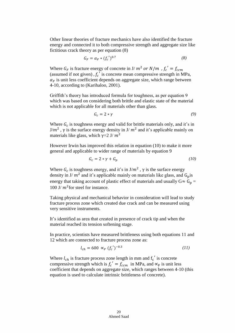
Other linear theories of fracture mechanics have also identified the fracture
energy and connected it to both compressive strength and aggregate size like
fictitious crack theory as per equation (8)
𝐺𝐹 = 𝛼𝐹 ∗ (𝑓𝑐′)0.7 (8)
Where 𝐺𝐹 is fracture energy of concrete in J/ 𝑚2 𝑜𝑟 𝑁/𝑚 , 𝑓𝑐′ = 𝑓𝑐𝑐𝑚
(assumed if not given) , 𝑓𝑐′ is concrete mean compressive strength in MPa,
𝛼𝐹 is unit less coefficient depends on aggregate size, which range between
4-10, according to (Karihaloo, 2001).
Griffith’s theory has introduced formula for toughness, as per equation 9
which was based on considering both brittle and elastic state of the material
which is not applicable for all materials other than glass.
𝐺𝑐 = 2 ∗ 𝛾 (9)
Where 𝐺𝑐 is toughness energy and valid for brittle materials only, and it’s in
J/𝑚2 , γ is the surface energy density in J/ 𝑚2 and it’s applicable mainly on
materials like glass, which γ=2 J/ 𝑚2
However Irwin has improved this relation in equation (10) to make it more
general and applicable to wider range of materials by equation 9
𝐺𝑐 = 2 ∗ 𝛾 + 𝐺𝑝 (10)
Where 𝐺𝑐 is toughness energy, and it’s in J/𝑚2 , γ is the surface energy
density in J/ 𝑚2 and it’s applicable mainly on materials like glass, and Gpis
energy that taking account of plastic effect of materials and usually G≈ Gp =
100 J/ 𝑚2for steel for instance.
Taking physical and mechanical behavior in consideration will lead to study
fracture process zone which created due crack and can be measured using
very sensitive instruments.
It’s identified as area that created in presence of crack tip and when the
material reached its tension softening stage.
In practice, scientists have measured brittleness using both equations 11 and
12 which are connected to fracture process zone as:
𝑙𝑐ℎ = 600 ∝𝐹 (𝑓𝑐′)−0.3 (11)
Where 𝑙𝑐ℎ is fracture process zone length in mm and fc′ is concrete
compressive strength which is 𝑓𝑐′ = 𝑓𝑐𝑐𝑚 in MPa, and ∝F is unit less
coefficient that depends on aggregate size, which ranges between 4-10 (this
equation is used to calculate intrinsic brittleness of concrete).
21
Ahmed Saad
Intrinsic brittleness means that the brittleness is given priority as property
because it’s inherent property of concrete unlike extrinsic properties that
could be due to temporary conditions.
So, the observation that compressive strength increase by decreasing 𝑙𝑐ℎ ,
while the relation was observed that both 𝑙𝑐ℎ and ∝F will increase if any one
of them increased and vice versa.
It has been noticed also that 𝑙𝑐ℎ is similar to 𝑙𝑝 in both magnitude and
definition as per equation 12
𝑙𝑝 = (𝐸′ ∗ 𝐺𝐹)/𝑓𝑡′2
(12)
Where 𝑙𝑝 is fracture process zone length which equal to between (200-500
mm for normal concrete less than 50 MPa), 𝐺𝐹 is fracture energy in J/
𝑚2 𝑜𝑟 𝑁/𝑚, 𝐸′ is modulus of elasticity (young’s modulus) in plane stress
according to Griffith’s theory, GPa, and 𝑓𝑡′ is uniaxial tensile strength limit
of the material, or attained tensile strength of material in MPa, and its
equivalent to concrete mean tensile strength 𝑓𝑐𝑡𝑚 , 𝑓𝑡′ = 𝑓𝑐𝑡𝑚 (assumed if
not given).
3.5.3 Empirical relation between strength parameters in concrete
In practice, there are many ways to simulate cracks growth by finite
elements modelling using discrete, and smeared modelling, and measuring
cracks experimentally by crack tip opening displacement (CTOD) which is
used to measure a wide range of materials whether, elastic-plastic or quasi-
brittle like concrete, or by using R-curve which represents crack growth
resistance curve (Karihaloo, 2001).
However, these methods require special instruments that not available for
this study.
Note here that sometimes, special abbreviations will be used in this section
and next one to ease understating the equations like 𝑓𝑐𝑡𝑚
and 𝑓𝑐𝑐𝑡 for shorting
the meaning.
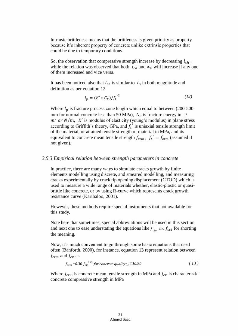
Now, it’s much convenient to go through some basic equations that used
often (Banforth, 2000), for instance, equation 13 represent relation between
𝑓𝑐𝑡𝑚 and 𝑓𝑐𝑘 as
𝑓𝑐𝑡𝑚=0.30 𝑓𝑐𝑘2/3
for concrete quality ≤ C50/60 ( 13 )
Where 𝑓𝑐𝑡𝑚 is concrete mean tensile strength in MPa and 𝑓𝑐𝑘 is characteristic
concrete compressive strength in MPa
22
Ahmed Saad
So, from 𝑓𝑐𝑡𝑚 it’s easy to obtain mean flexural 𝑓𝑓𝑡𝑚 as per equation (14),
according to (Banforth, 2000)
𝑓𝑓𝑡𝑚 = ℎ𝑖𝑔ℎ𝑒𝑟 𝑜𝑓 {(1.6 −
ℎ
1000) 𝑓𝑐𝑡𝑚
𝑓𝑐𝑡𝑚
(14)
Where both fftm and fctm are in MPa, fftm is concrete mean tensile strength
and fftm is concrete mean flexural strength.
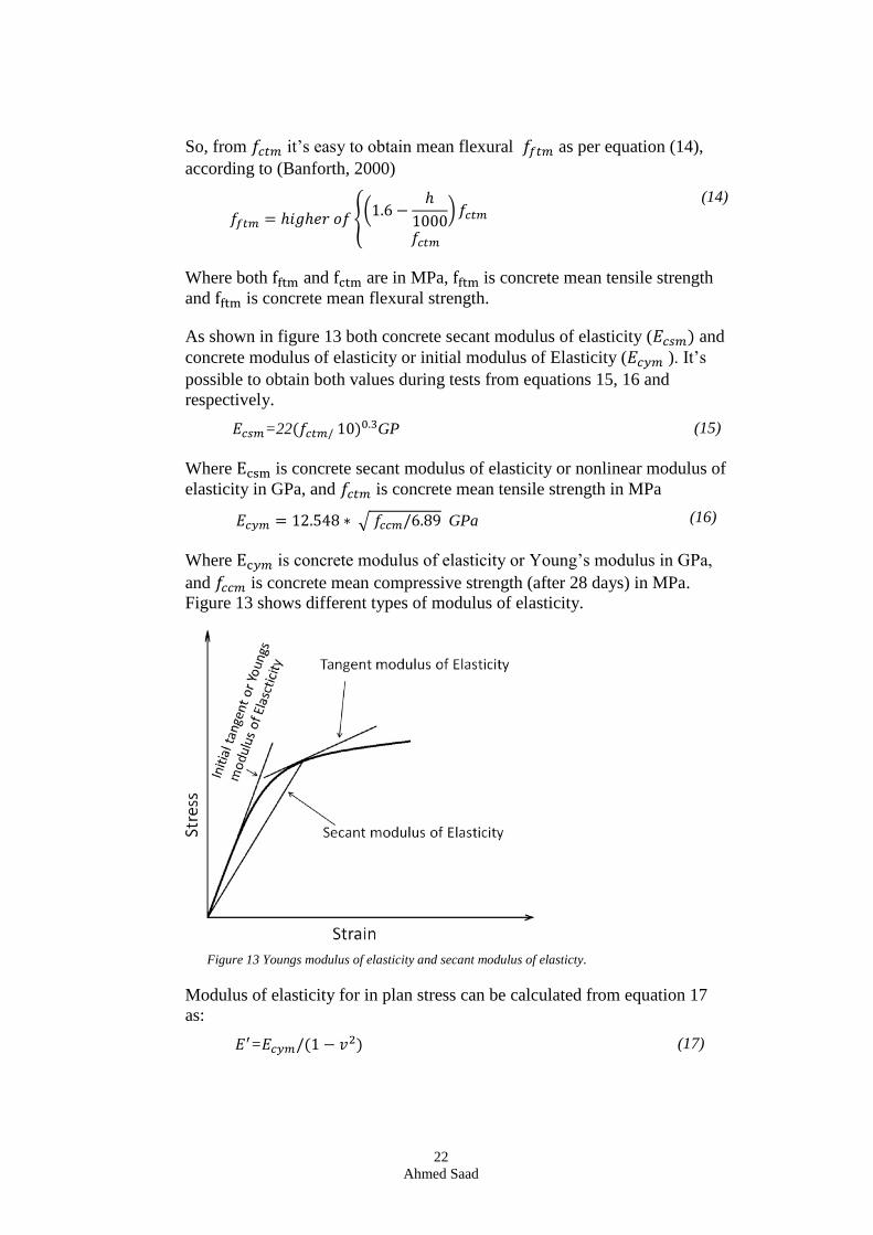
As shown in figure 13 both concrete secant modulus of elasticity (𝐸𝑐𝑠𝑚) and
concrete modulus of elasticity or initial modulus of Elasticity (𝐸𝑐𝑦𝑚 ). It’s
possible to obtain both values during tests from equations 15, 16 and
respectively.
𝐸𝑐𝑠𝑚=22(𝑓𝑐𝑡𝑚/ 10)0.3GP (15)
Where Ecsm is concrete secant modulus of elasticity or nonlinear modulus of
elasticity in GPa, and 𝑓𝑐𝑡𝑚 is concrete mean tensile strength in MPa
𝐸𝑐𝑦𝑚 = 12.548 ∗ √ 𝑓𝑐𝑐𝑚/6.89 GPa (16)
Where Ec𝑦𝑚 is concrete modulus of elasticity or Young’s modulus in GPa,
and 𝑓𝑐𝑐𝑚 is concrete mean compressive strength (after 28 days) in MPa.
Figure 13 shows different types of modulus of elasticity.
Figure 13 Youngs modulus of elasticity and secant modulus of elasticty.
Modulus of elasticity for in plan stress can be calculated from equation 17
as:
𝐸′=𝐸𝑐𝑦𝑚/(1 − 𝑣2) (17)
23
Ahmed Saad
Where 𝐸′ is modulus of elasticity (young’s modulus) in plane stress
according to Griffith’s theory 𝑣 is unit less Poisson’s ratio.
3.5.4 Equations for evaluation of experimental test
According to (Banforth, 2000), compression tests for cylinder specimens are
using basic equation (18)
𝑓𝑐𝑐𝑡 = 𝐹/𝐴 (18)
Where 𝑓𝑐𝑐𝑡 is compressive strength based on test in MPa, 𝐹 is failure load, A
is cross-sectional area of sample and equal to 𝜋r2 for cylinder in meter, r is
radius of cylinder for a sample in meter.
Direct tension test for cylinder test is using equations (19) and (20)
𝑓𝑐𝑡𝑡 = 𝐹/𝐴 (19)
Where 𝑓𝑐𝑡𝑡 is tensile strength based on test in MPa, 𝐹 is failure load, A is
cross-sectional area of sample and equal to bd for rectangular, b and are
dimensions parameters for rectangular shape cross-section in meter..
ε= ΔL/L (20)
Where ε is longitudinal strain and its unit less, ΔL is change of sample
length in meter; L is original length in meter.
Equation (20) is applicable also to both compression and tension tests.
Tension splitting test is using equation (21),
𝑓𝑏𝑡=2F/𝜋𝐷𝐿 (21)
Where 𝑓𝑏𝑡 is tensile strength for splitting tension test based on (Brazilian
test) in MPa, F is failure load, D is specimen diameter in m, L is specimen
length in m.
Theoretical value of tensile strength of direct can be computed from for
splitting tension test by equation (22), according to (Banforth, 2000)
𝑓𝑐𝑡=0.9 𝑓𝑏𝑡 (22)
Where 𝑓𝑐𝑡 is tensile strength of direct tension test in MPa, 𝑓𝑏𝑡 is tensile
strength for splitting tension test (Brazilian test) in MPa
Relation between tension splitting strength and compressive strength
according to Olukun, (Riera, et al., 2014), can be shown in equation 23 as:
𝑓𝑏𝑘=0.295 (𝑓𝑐𝑘 )0.69 (23)
24
Ahmed Saad
Where 𝑓𝑏𝑘 is characteristic tensile strength for splitting tension test
(Brazilian test) in MPa, and 𝑓𝑐𝑘 is characteristic concrete compressive
strength in MPa
Olukun has written another relation to represent both characteristic direct
tensile strength fctk and characteristic compressive strength 𝑓𝑐𝑘 as:
𝑓𝑐𝑡𝑘=2.017 +0.068 𝑓𝑐𝑘 (24)
Where fctk is characteristic direct tensile strength in MPa, and 𝑓𝑐𝑘 is
characteristic compressive strength in MPa.
And even relation between fctk and 𝑓𝑐𝑘 can be checked in range by equation
25 as:
0.95(𝑓𝑐𝑘/ 𝑓𝑐0 )2/3 ≤ 𝑓𝑐𝑡𝑘 ≤ 1.85(𝑓𝑐𝑘/ 𝑓𝑐0 )
2/3 (25)
Where fctk is characteristic direct tensile strength in MPa, and 𝑓𝑐𝑘 is
characteristic compressive strength in MPa, and fc0 = 10 MPa (constant).
3.5.5 Stresses in Brazilian test
To calculate stresses and shear in any given point or any point at path that
locates in the circle-shape specimen of Brazilian tension test with applied
load infinitesimal or very small area, equation 27 is applicable according
Dr.h.c.H ,(TUW)as
𝜎𝑥=2P/πl⌊(𝑅 − 𝑦)𝑥2/𝑟14 + (𝑅 + 𝑦)𝑥2/𝑟2
4− 1/𝑑⌋
𝜎𝑦=- 2P/πl⌊(𝑅 − 𝑦)3/𝑟14 + (𝑅 + 𝑦)3/𝑟2
4− 1/𝑑⌋
𝜎𝑥𝑦=2P/πl∗ ⌊(𝑅 − 𝑦)2𝑥 /𝑟14 + (𝑅 + 𝑦)2𝑥 /𝑟2
4⌋
(26)
Where 𝜎𝑥 is normal stress in x-direction in MPa, 𝜎𝑦 is normal stress in y-
direction in MPa, and 𝜎𝑥𝑦 is shear stress in MPa, 𝑟1 and 𝑟2 are distance
between top and bottom of y-axis from point accordingly, R is radius of
Brazilian disc, d is diameter of disc, y is coordinate of point over y-axis, and
P and l are load in kN and depth of Brazilian tension splitting specimen in
m. See figure 14.
25
Ahmed Saad
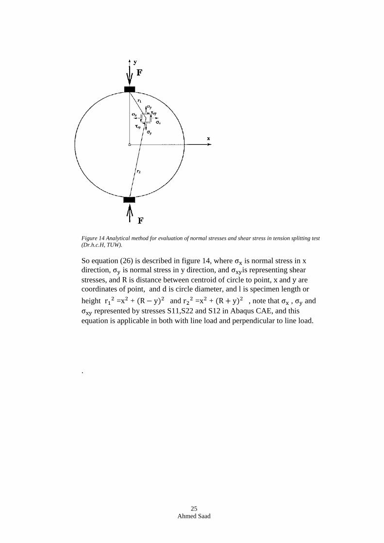
Figure 14 Analytical method for evaluation of normal stresses and shear stress in tension splitting test
(Dr.h.c.H, TUW).
So equation (26) is described in figure 14, where σx is normal stress in x
direction, σy is normal stress in y direction, and σxyis representing shear
stresses, and R is distance between centroid of circle to point, x and y are
coordinates of point, and d is circle diameter, and l is specimen length or
height r12 =x2 + (R − y)2 and r2
2 =x2 + (R + y)2 , note that σx , σy and
σxy represented by stresses S11,S22 and S12 in Abaqus CAE, and this
equation is applicable in both with line load and perpendicular to line load.
.
26
Ahmed Saad
4. Method
In bridges, there are many ways to investigate both stresses and cracks
propagation in terms of both materials and geometry, and this thesis will
focus on some useful methods to do that.
According to Eurocode 2, both splitting tension test and uniaxial tension test
have been used and the result was that tensile strength that obtained from
uniaxial tension test was 90% of that obtained by splitting tension test.
However, uniaxial tension test is not enough alone because of the fact that
concrete has low tensile strength, and therefore it’s sensitive to test
conditions like eccentricity.
For cracks control, tension tests are very important to be done because they
are deciding the weakest property of concrete that cause the cracks.
However, compression test is vital test that could give important mechanical
properties for concrete, for instance modulus of elasticity.
In this study, all of three tests: uniaxial compression, uniaxial tension and
splitting tension tests will be performed in LNU laboratory and modelled
using FE modeling. Furthermore, modeling for concrete slab similar to that
used in bridges will be simulated using Abaqus.
4.1 Experimental tests
To understand the behavior of concrete slab under loading, some
experiments on laboratory can be done on very small specimens: cylinder
compression test, dog-bone direct tension test, flexural test, CTOD test
(crack tip opening displacement) and Brazilian tension splitting test.
However, some tests will be excluded from this study and only uniaxial
compression, tension and splitting tension tests will be performed.
For the purpose of understanding the mechanical material properties of
concrete in bridges, three tests: uniaxial compression, tension and splitting
tension tests will be performed to understand failure pattern, stress and
strains for every test.
It’s important to mention that the surface that researcher is interested to
study, must be sprayed before with both black and white spray, see
appendix. This give dense visible texture or surface of black particles that
ARAMIS cameras can observe, see figure 20 in the results chapter.
All experimental tests were observed by ARAMIS cameras system that
gives shots to specimen in terms of stages, and program (GOM Correlate
Professional V8 SR1) has been used to process the results, see figures 25, 30
27
Ahmed Saad
and appendix 4. The set-up was up to 500 stages, these excellent cameras
could record specimen situation for almost all particles in surface that
researcher interested for any specimen.
Furthermore, digital caliber has been used in all tests to measure in accurate
manner, see appendix. All experimental tests will be performed using MTS-
810, see appendix.
4.1.1 Brazilian splitting tension (brazilin test)
A cylinder- specimen will be examined under loading until failure using
MTS-810, and same class used in bridges.
Very thin teflon piece will be used between loading platen and specimen to
smooth out and minimize surface stress.
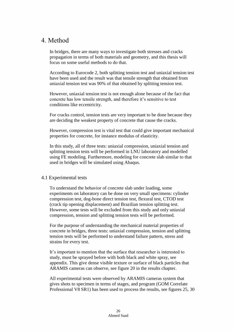
Time, displacement control rate (0.5 mm/min) and load will be recorded for
each specimen. Thereafter, tensile strength will be calculated. Figure 15
shows sectional plan for test and boundary conditions
.
Figure 15 Sectional plan view for tension splitting (Brazilian test).
4.1.2 Uniaxial compression test
Uniaxial compression test will be performed for cylinder specimens until
failure.
A fiber board of 3 mm will be used between loading platen and specimen,
to absorb any uneven surface due to mistakes of manufacturing.
28
Ahmed Saad
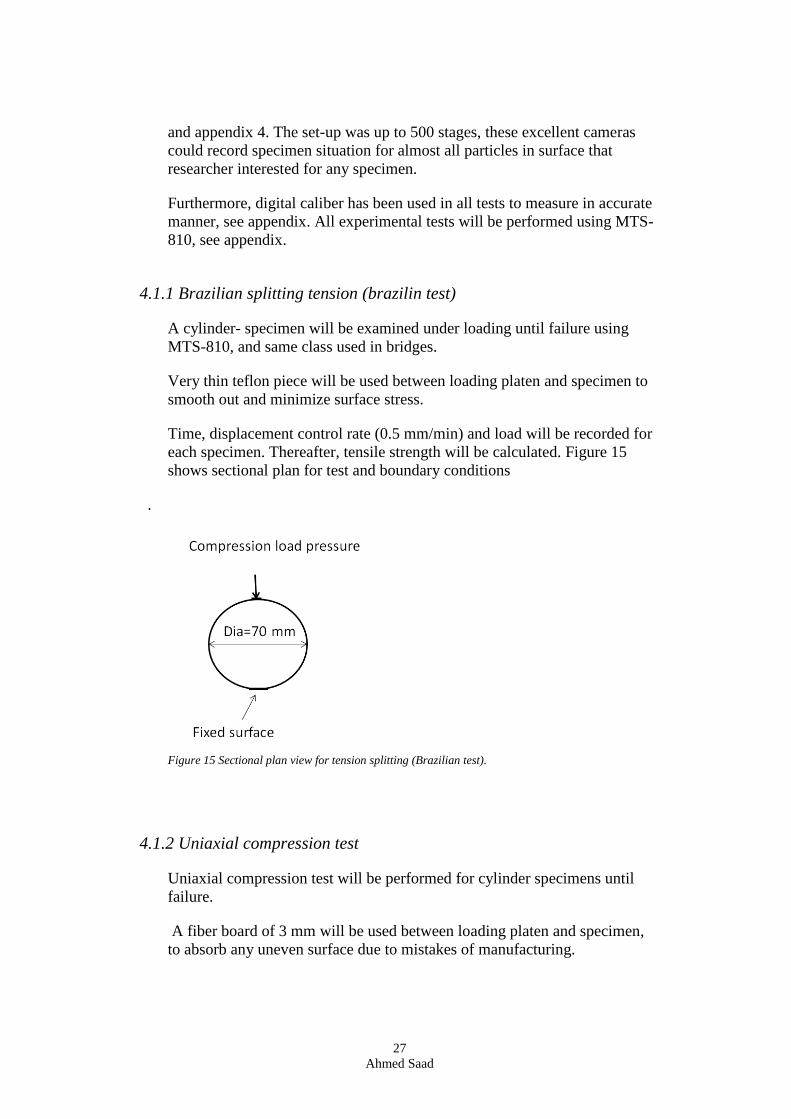
Time, displacement control rate (0.5-0.8 mm/min), and load will be recorded
for each specimen. Thereafter, uniaxial compressive strength will be
calculated. Figure 16 shows sectional plan for test and boundary conditions.
Figure 16 Sectional plan view for compression test.
4.1.3 Direct uniaxial tension test
Uniaxial tension test will be performed for a dog-bone specimen until
failure. This will be performed in the laboratory of LNU using same class of
concrete C30/37 or (C32/40) locally, which is same class that used in
bridges by machine MTS-810 material test system.
An embedded steel bars will be used to transfer load to concrete specimen
and some reinforcements will be provided for both ends of specimen to
support embedded bars and to protect from the effect of shear stress that
could happen for such shape.
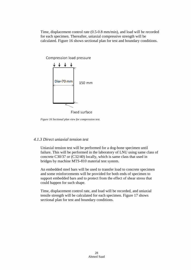
Time, displacement control rate, and load will be recorded, and uniaxial
tensile strength will be calculated for each specimen. Figure 17 shows
sectional plan for test and boundary conditions.
29
Ahmed Saad
Figure 17 Sectional plan view for uniaxial tension test.
4.2 Finite element modelling (FEM)
Concrete is a heterogeneous material and it reacts in both linear and non-
linear way to applied load, so a finite element modelling to simulate
concrete is used in both cases based on purpose of study.
Finite element modelling is general method that used the basis of dividing
materials into elements called finite elements.
In this study, only linear modelling for concrete slab will be simulated for
different skew angles using Abaqus, so Misses stresses will be known at
each corner for every slab. This modelling will give idea about geometry
part.
4.2.1 Linear behavior of concrete in FEM
To simulate reinforced concrete structures or concrete structures, some basic
parameters should be used such as modulus of elasticity (Young’s modulus)
and Poisons ratio, as well geometry and load in kN/m2 or MPa.
30
Ahmed Saad
The load may be applied in different ways depending on purpose. However,
linear behavior approach using Abaqus , is good to define stresses
distribution in slabs and other concrete structures and give preliminary study
to measure crack propagation. Although, this approach is not adequate to
represent real behavior of concrete and how cracks propagates due to
existing of softening in fracture process zone and other parameters.
4.3 Analytical method
To understand the concept of cracks and what will happen to material
(concrete in this case), an analytical method using equations (26) will be
compared with Abaqus results to study normal stresses and shear stresses in
some specimens (Brazilian test specimens).
4.4 Stresses at corners of slabs with geometry change
Stresses in four angles in corners will be investigated to study and compare
skewness on stresses in slabs of bridges. This will be done by modelling of
slabs 1*2 m2 using Abaqus CAE. Thus, this is for a purpose to model slabs
in different angles in bridge system.
31
Ahmed Saad
5. Results
5.1 Experimental and crack propagations results
5.1.1 Brazilian splitting tension test
The Brazilaian splitting tension test is test that give strength of concrete
when its subjected for compression .
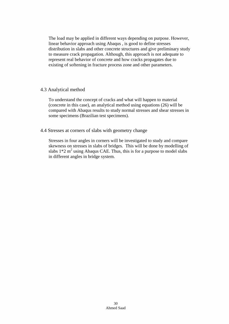
The experiment has been performed for several specimens under loading
using MTS-810 , see figure 18.
Figure 18 Setup for splitting tension test (Brazilian).
This test is one efficient way to study the behavior of concrete structures
because it shows the attitude of concrete cylinder with no effect of
eccentricity, therefore it’s more accurate.
Three specimens have been tested, see table 3 and using equation (21),
fbt=2F/πDL , for instance for first specimen, represents
fbt=30*103/( 𝜋*(69.63/2)*153.4*106) = 1.787*106 [N/ 𝑀2], or1.787
Its displacement control loading that have been used in all tests and actually
splitting tension test was calibrated by rate of 0.5 mm/min, actually its very
slow loading because crack propagations occur at very small value in
concrete compared with compression failure.
32
Ahmed Saad
Table 3 Brazilian Splitting tension test for specimens with different classes
Spec.
Sr.No.
Specimen
dimensions(average
diameter, length)
mm
Ultimate
load
(kN)
Displacement
control rate
(mm/min.)
Measured
Tensile
stress/
strength
MPa
1 (69.63,153.45) 30 0.5 1.787
2 (69.89,152.25) 54.14 0.5 3.239
3 (69.77,153.13) 48.64 0.5 2.898
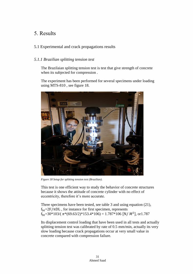
This test has been done using teflon pieces in both top and bottom as shown
in figure 19 to smooth out surface stresses that could arise between steel
platens and concrete specimen.
Figure 19 Splitting tension specimen with teflon.
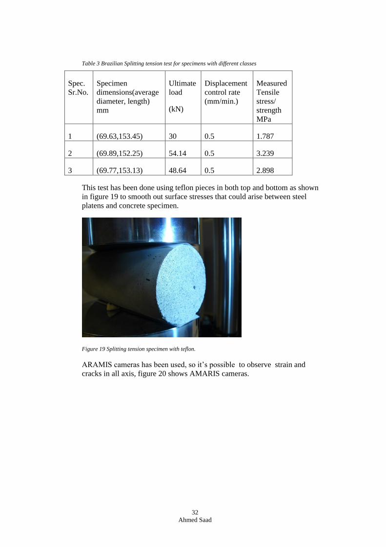
ARAMIS cameras has been used, so it’s possible to observe strain and
cracks in all axis, figure 20 shows AMARIS cameras.
33
Ahmed Saad
Figure 20 ARAMIS cameras have been used in tests to detect crack propagation.
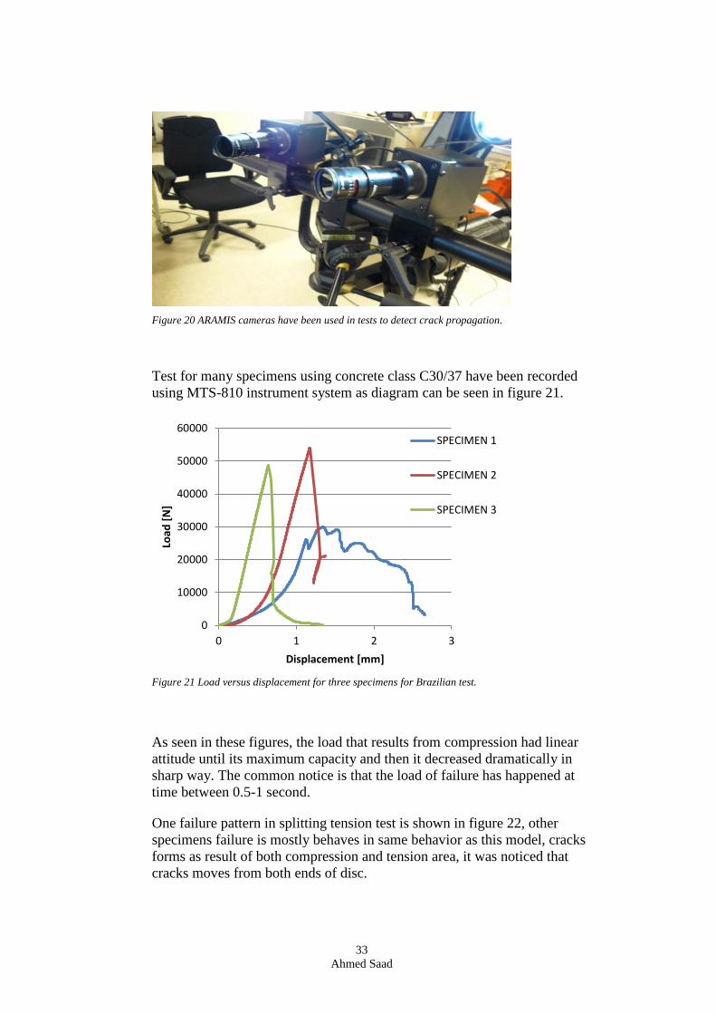
Test for many specimens using concrete class C30/37 have been recorded
using MTS-810 instrument system as diagram can be seen in figure 21.
Figure 21 Load versus displacement for three specimens for Brazilian test.
As seen in these figures, the load that results from compression had linear
attitude until its maximum capacity and then it decreased dramatically in
sharp way. The common notice is that the load of failure has happened at
time between 0.5-1 second.
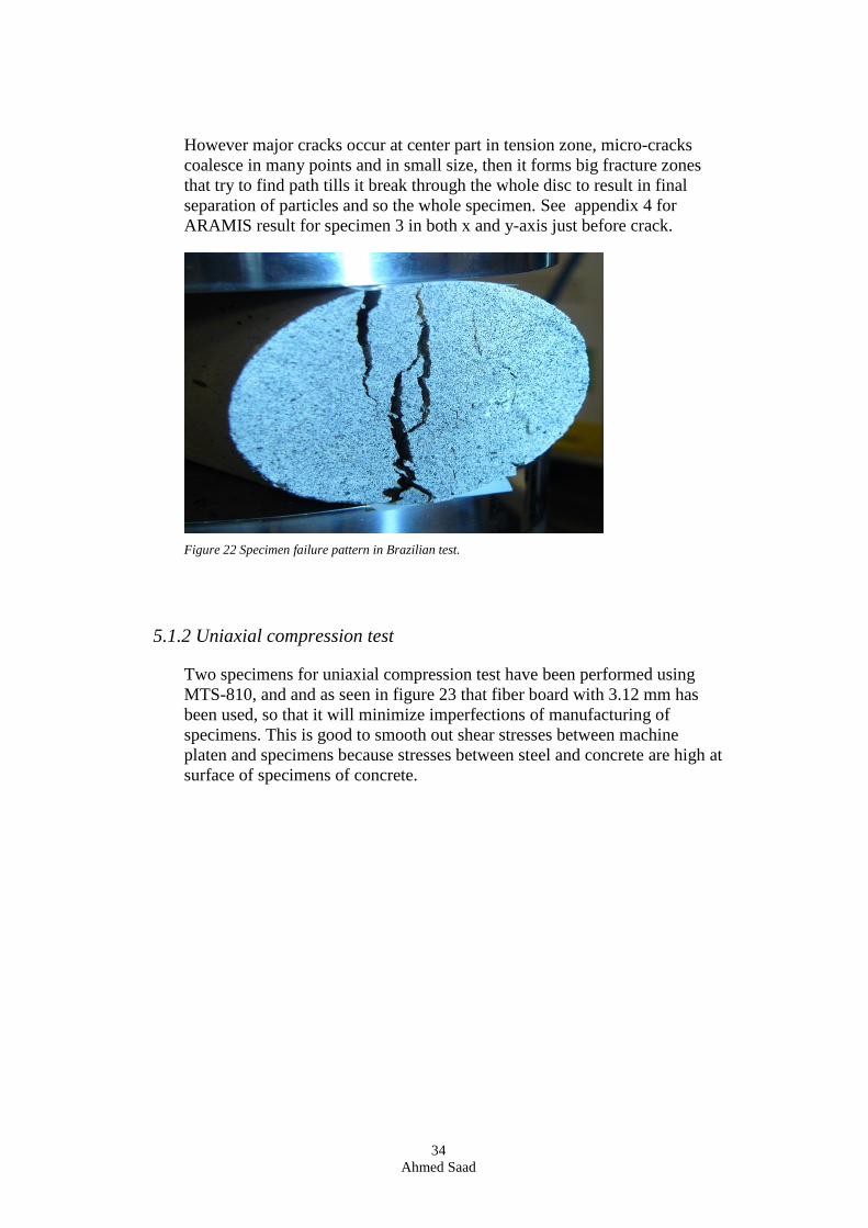
One failure pattern in splitting tension test is shown in figure 22, other
specimens failure is mostly behaves in same behavior as this model, cracks
forms as result of both compression and tension area, it was noticed that
cracks moves from both ends of disc.
0
10000
20000
30000
40000
50000
60000
0 1 2 3
Load
[N
]
Displacement [mm]
SPECIMEN 1
SPECIMEN 2
SPECIMEN 3
34
Ahmed Saad
However major cracks occur at center part in tension zone, micro-cracks
coalesce in many points and in small size, then it forms big fracture zones
that try to find path tills it break through the whole disc to result in final
separation of particles and so the whole specimen. See appendix 4 for
ARAMIS result for specimen 3 in both x and y-axis just before crack.
Figure 22 Specimen failure pattern in Brazilian test.
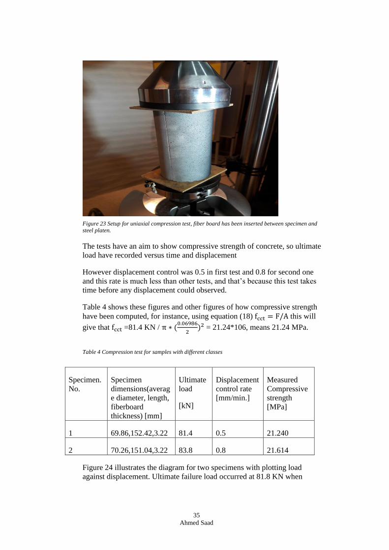
5.1.2 Uniaxial compression test
Two specimens for uniaxial compression test have been performed using
MTS-810, and and as seen in figure 23 that fiber board with 3.12 mm has
been used, so that it will minimize imperfections of manufacturing of
specimens. This is good to smooth out shear stresses between machine
platen and specimens because stresses between steel and concrete are high at
surface of specimens of concrete.
35
Ahmed Saad
Figure 23 Setup for uniaxial compression test, fiber board has been inserted between specimen and
steel platen.
The tests have an aim to show compressive strength of concrete, so ultimate
load have recorded versus time and displacement
However displacement control was 0.5 in first test and 0.8 for second one
and this rate is much less than other tests, and that’s because this test takes
time before any displacement could observed.
Table 4 shows these figures and other figures of how compressive strength
have been computed, for instance, using equation (18) fcct = F/A this will
give that fcct =81.4 KN / π ∗ (0.06986
2)2 = 21.24*106, means 21.24 MPa.
Table 4 Compression test for samples with different classes
Specimen.
No.
Specimen
dimensions(averag
e diameter, length,
fiberboard
thickness) [mm]
Ultimate
load
[kN]
Displacement
control rate
[mm/min.]
Measured
Compressive
strength
[MPa]
1 69.86,152.42,3.22 81.4 0.5 21.240
2 70.26,151.04,3.22 83.8 0.8 21.614
Figure 24 illustrates the diagram for two specimens with plotting load
against displacement. Ultimate failure load occurred at 81.8 KN when
36
Ahmed Saad
displacement was 1.5 mm, while the second specimen’s failure load has
occurred at 2.5 mm.
Figure 24 Load versus displacement for two specimens for uniaxial compression test
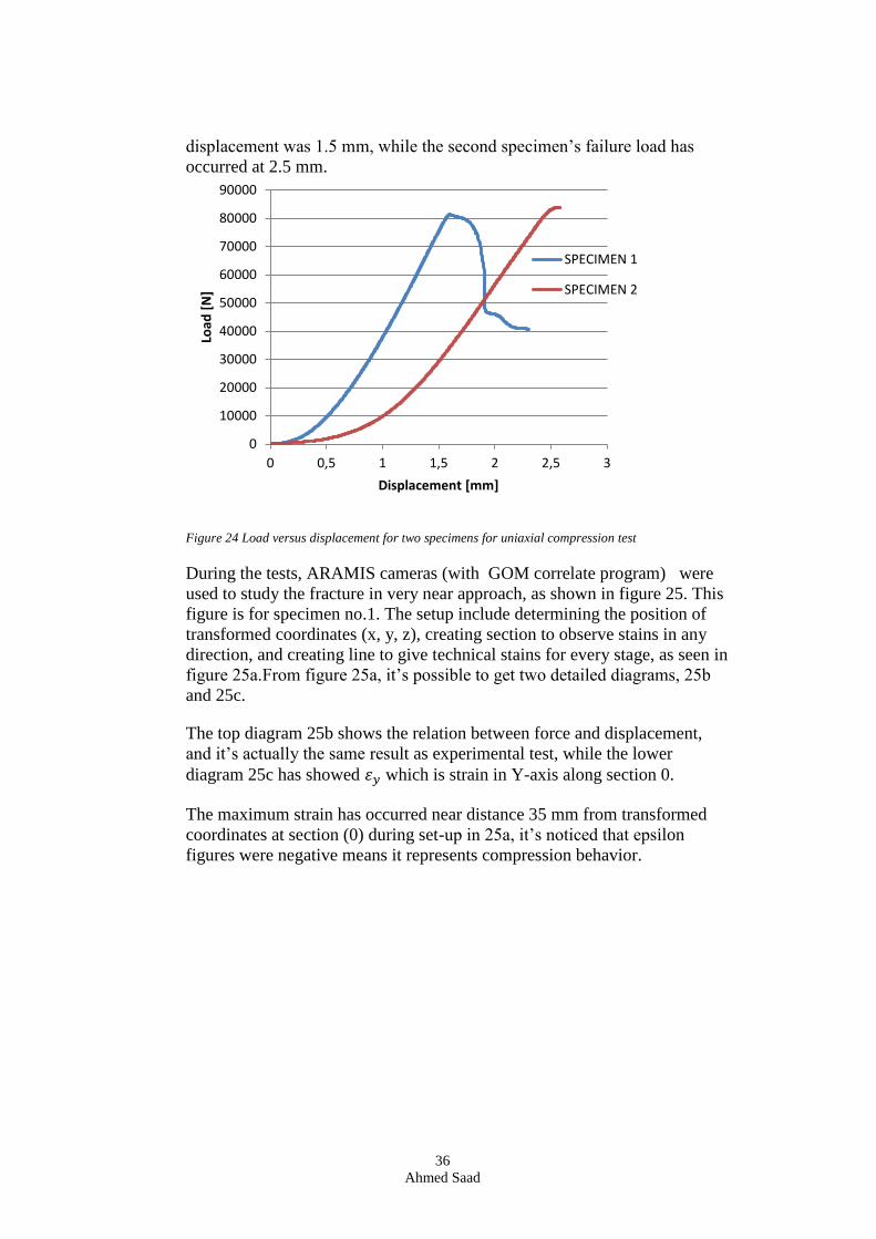
During the tests, ARAMIS cameras (with GOM correlate program) were
used to study the fracture in very near approach, as shown in figure 25. This
figure is for specimen no.1. The setup include determining the position of
transformed coordinates (x, y, z), creating section to observe stains in any
direction, and creating line to give technical stains for every stage, as seen in
figure 25a.From figure 25a, it’s possible to get two detailed diagrams, 25b
and 25c.
The top diagram 25b shows the relation between force and displacement,
and it’s actually the same result as experimental test, while the lower
diagram 25c has showed 𝜀𝑦 which is strain in Y-axis along section 0.
The maximum strain has occurred near distance 35 mm from transformed
coordinates at section (0) during set-up in 25a, it’s noticed that epsilon
figures were negative means it represents compression behavior.
0
10000
20000
30000
40000
50000
60000
70000
80000
90000
0 0,5 1 1,5 2 2,5 3
Load
[N
]
Displacement [mm]
SPECIMEN 1
SPECIMEN 2
37
Ahmed Saad
Figure 25 Section analysis using Aramis photo for specimen No.1 (compression test) (a) deformations
scanning with transformed coordinates and defined section o and line 1 (b) Force versus
displacement along section 0 (c) strain in y-direction along section 0.
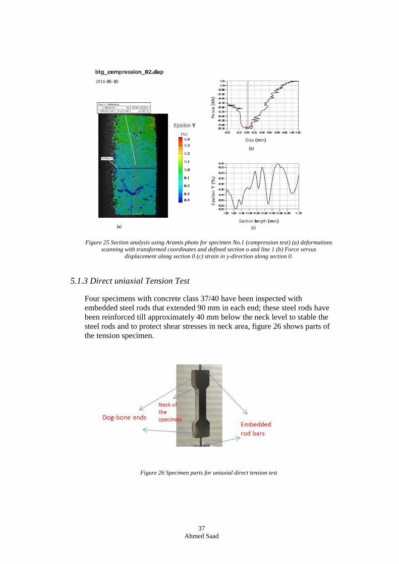
5.1.3 Direct uniaxial Tension Test
Four specimens with concrete class 37/40 have been inspected with
embedded steel rods that extended 90 mm in each end; these steel rods have
been reinforced till approximately 40 mm below the neck level to stable the
steel rods and to protect shear stresses in neck area, figure 26 shows parts of
the tension specimen.
Figure 26 Specimen parts for uniaxial direct tension test
38
Ahmed Saad
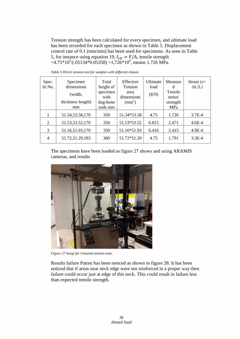
Tension strength has been calculated for every specimen, and ultimate load
has been recorded for each specimen as shown in Table 5. Displacement
control rate of 0.1 (mm/min) has been used for specimens. As seen in Table
5, for instance using equation 19, fctt = F/A, tensile strength
=4.75*103/(.05134*0.05358) =1,726*10
6, means 1.726 MPa.
Table 5 Direct tension test for samples with different classes
Spec.
Sr.No.
Specimen
dimensions
(width,
thickness length)
mm
Total
height of
specimen
with
dog-bone
ends mm
Effective
Tension
area
dimensions
(mm2)
Ultimate
load
(KN)
Measure
d
Tensile
stress/
strength
MPa
Strain (ε=
ΔL/L)
1 51.34,53.58,170 350 51.34*53.58 4.75 1.726 3.7E-4
2 51.53,53.52,170 350 51.53*53.52 6.815 2.471 4.6E-4
3 51.16,51.93,170 350 51.16*51.93 6.416 2.415 4.9E-4
4 51.72,51.29,183 360 51.72*51.29 4.75 1.791 3.3E-4
The specimens have been loaded as figure 27 shows and using ARAMIS
cameras, and results
Figure 27 Setup for Uniaxial tension tests.
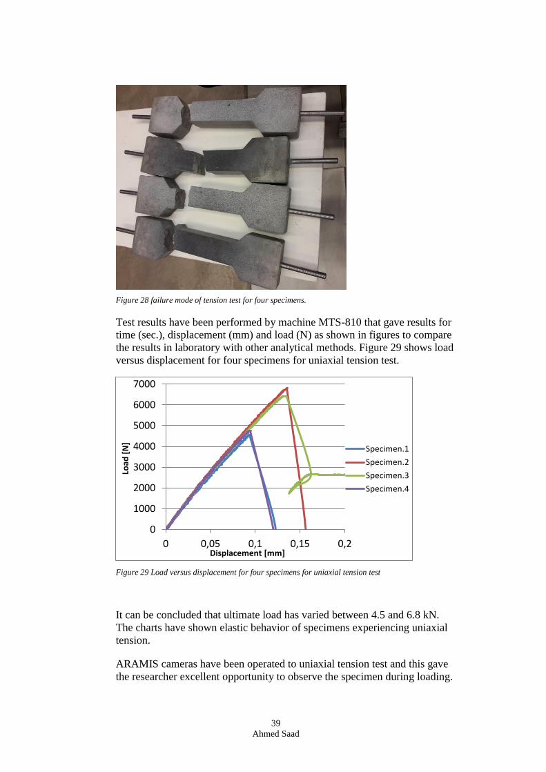
Results failure Patten has been noticed as shown in figure 28. It has been
noticed that if areas near neck edge were not reinforced in a proper way then
failure could occur just at edge of this neck. This could result in failure less
than expected tensile strength.
39
Ahmed Saad
Figure 28 failure mode of tension test for four specimens.
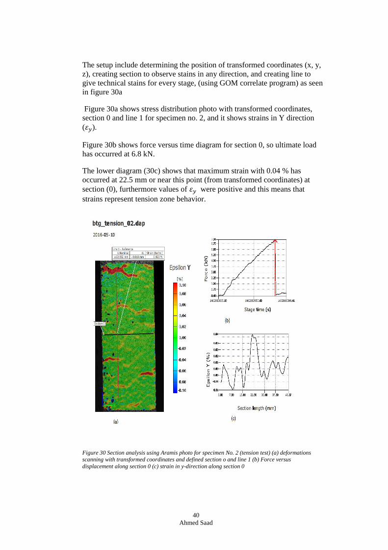
Test results have been performed by machine MTS-810 that gave results for
time (sec.), displacement (mm) and load (N) as shown in figures to compare
the results in laboratory with other analytical methods. Figure 29 shows load
versus displacement for four specimens for uniaxial tension test.
Figure 29 Load versus displacement for four specimens for uniaxial tension test
It can be concluded that ultimate load has varied between 4.5 and 6.8 kN.
The charts have shown elastic behavior of specimens experiencing uniaxial
tension.
ARAMIS cameras have been operated to uniaxial tension test and this gave
the researcher excellent opportunity to observe the specimen during loading.
0
1000
2000
3000
4000
5000
6000
7000
0 0,05 0,1 0,15 0,2
Load
[N
]
Displacement [mm]
Specimen.1
Specimen.2
Specimen.3
Specimen.4
40
Ahmed Saad
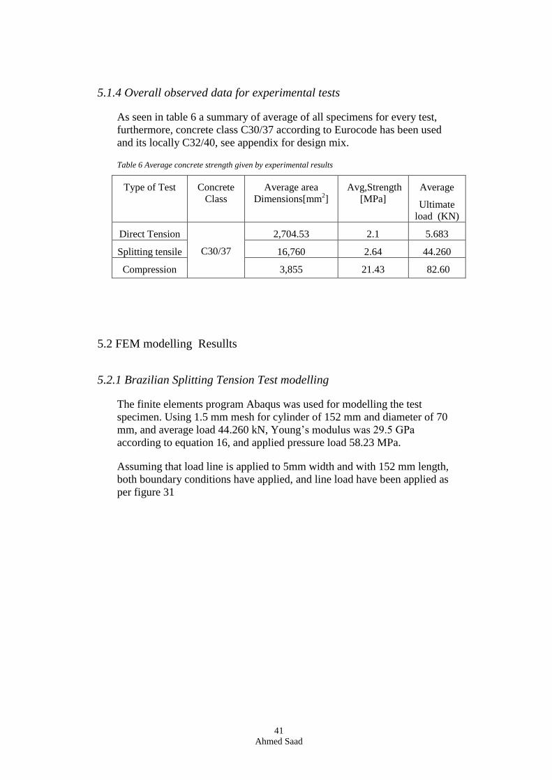
The setup include determining the position of transformed coordinates (x, y,
z), creating section to observe stains in any direction, and creating line to
give technical stains for every stage, (using GOM correlate program) as seen
in figure 30a
Figure 30a shows stress distribution photo with transformed coordinates,
section 0 and line 1 for specimen no. 2, and it shows strains in Y direction
(𝜀𝑦).
Figure 30b shows force versus time diagram for section 0, so ultimate load
has occurred at 6.8 kN.
The lower diagram (30c) shows that maximum strain with 0.04 % has
occurred at 22.5 mm or near this point (from transformed coordinates) at
section (0), furthermore values of 𝜀𝑦 were positive and this means that
strains represent tension zone behavior.
Figure 30 Section analysis using Aramis photo for specimen No. 2 (tension test) (a) deformations
scanning with transformed coordinates and defined section o and line 1 (b) Force versus
displacement along section 0 (c) strain in y-direction along section 0
41
Ahmed Saad
5.1.4 Overall observed data for experimental tests
As seen in table 6 a summary of average of all specimens for every test,
furthermore, concrete class C30/37 according to Eurocode has been used
and its locally C32/40, see appendix for design mix.
Table 6 Average concrete strength given by experimental results
Type of Test Concrete
Class
Average area
Dimensions[mm2]
Avg,Strength
[MPa]
Average
Ultimate
load (KN)
Direct Tension
C30/37
2,704.53 2.1 5.683
Splitting tensile 16,760 2.64 44.260
Compression 3,855 21.43 82.60
5.2 FEM modelling Resullts
5.2.1 Brazilian Splitting Tension Test modelling
The finite elements program Abaqus was used for modelling the test
specimen. Using 1.5 mm mesh for cylinder of 152 mm and diameter of 70
mm, and average load 44.260 kN, Young’s modulus was 29.5 GPa
according to equation 16, and applied pressure load 58.23 MPa.
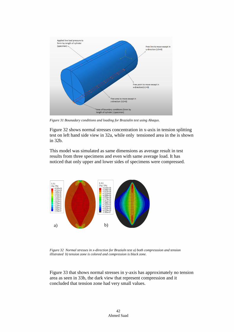
Assuming that load line is applied to 5mm width and with 152 mm length,
both boundary conditions have applied, and line load have been applied as
per figure 31
42
Ahmed Saad
Figure 31 Bounadary conditions and loading for Brazialin test using Abaqus.
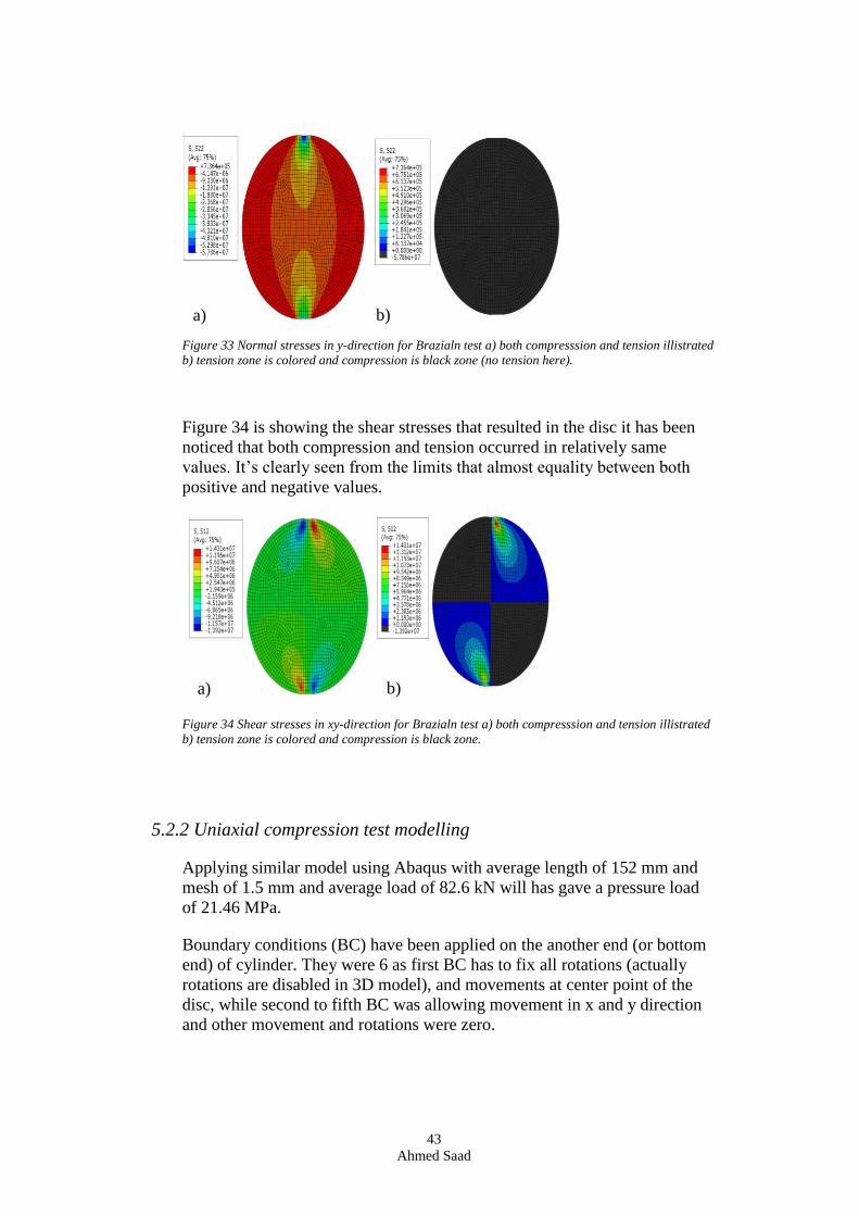
Figure 32 shows normal stresses concentration in x-axis in tension splitting
test on left hand side view in 32a, while only tensioned area in the is shown
in 32b.
This model was simulated as same dimensions as average result in test
results from three specimens and even with same average load. It has
noticed that only upper and lower sides of specimens were compressed.
Figure 32 Normal stresses in x-direction for Brazialn test a) both compresssion and tension
illistrated b) tension zone is colored and compression is black zone.
Figure 33 that shows normal stresses in y-axis has approximately no tension
area as seen in 33b, the dark view that represent compression and it
concluded that tension zone had very small values.
a) b)
43
Ahmed Saad
Figure 33 Normal stresses in y-direction for Brazialn test a) both compresssion and tension illistrated
b) tension zone is colored and compression is black zone (no tension here).
Figure 34 is showing the shear stresses that resulted in the disc it has been
noticed that both compression and tension occurred in relatively same
values. It’s clearly seen from the limits that almost equality between both
positive and negative values.
Figure 34 Shear stresses in xy-direction for Brazialn test a) both compresssion and tension illistrated
b) tension zone is colored and compression is black zone.
5.2.2 Uniaxial compression test modelling
Applying similar model using Abaqus with average length of 152 mm and
mesh of 1.5 mm and average load of 82.6 kN will has gave a pressure load
of 21.46 MPa.
Boundary conditions (BC) have been applied on the another end (or bottom
end) of cylinder. They were 6 as first BC has to fix all rotations (actually
rotations are disabled in 3D model), and movements at center point of the
disc, while second to fifth BC was allowing movement in x and y direction
and other movement and rotations were zero.
a) b)
a) b)
44
Ahmed Saad
Final BC has to be fixed in a chosen picked point in its direction and it was
x-axis in this case and allowed to move in y- directions and not allowed to
move in z-direction nor rotate. In fact this point is important to represent
actual situation of uniaxial compression test.
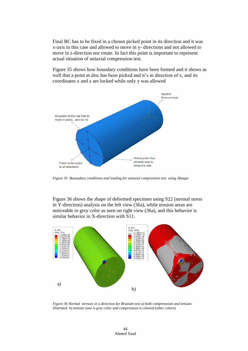
Figure 35 shows how boundary conditions have been formed and it shows as
well that a point at disc has been picked and it’s in direction of x, and its
coordinates x and z are locked while only y was allowed
Figure 35 Bounadary conditions and loading for uniaxial compression test using Abaqus
Figure 36 shows the shape of deformed specimen using S22 (normal stress
in Y-direction) analysis on the left view (36a), while tension areas are
noticeable in grey color as seen on right view (36a), and this behavior is
similar behavior in X-direction with S11.
Figure 36 Normal stresses in y-direction for Brazialn test a) both compresssion and tension
illistrated b) tension zone is grey color and compression is colored (other colors)
a) b)
45
Ahmed Saad
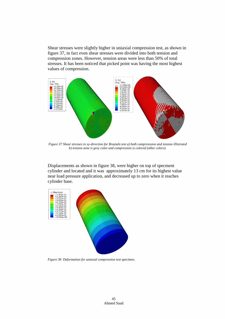
Shear stresses were slightly higher in uniaxial compression test, as shown in
figure 37, in fact even shear stresses were divided into both tension and
compression zones. However, tension areas were less than 50% of total
stresses. It has been noticed that picked point was having the most highest
values of compression.
Figure 37 Shear stresses in xy-direction for Brazialn test a) both compresssion and tension illistrated
b) tension zone is grey color and compression is colored (other colors).
Displacements as shown in figure 38, were higher on top of specment
cylinder and located and it was approximately 13 cm for its highest value
near load pressure application, and decreased up to zero when it reaches
cylinder base.
Figure 38 Deformation for uniaxial compression test specimen.
46
Ahmed Saad
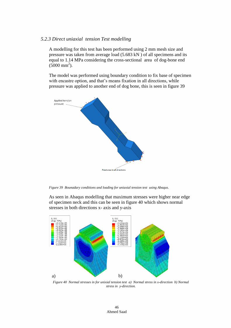
5.2.3 Direct uniaxial tension Test modelling
A modelling for this test has been performed using 2 mm mesh size and
pressure was taken from average load (5.683 kN ) of all specimens and its
equal to 1.14 MPa considering the cross-sectional area of dog-bone end
(5000 mm2).
The model was performed using boundary condition to fix base of specimen
with encastre option, and that’s means fixation in all directions, while
pressure was applied to another end of dog bone, this is seen in figure 39
Figure 39 Bounadary conditions and loading for uniaxial tension test using Abaqus.
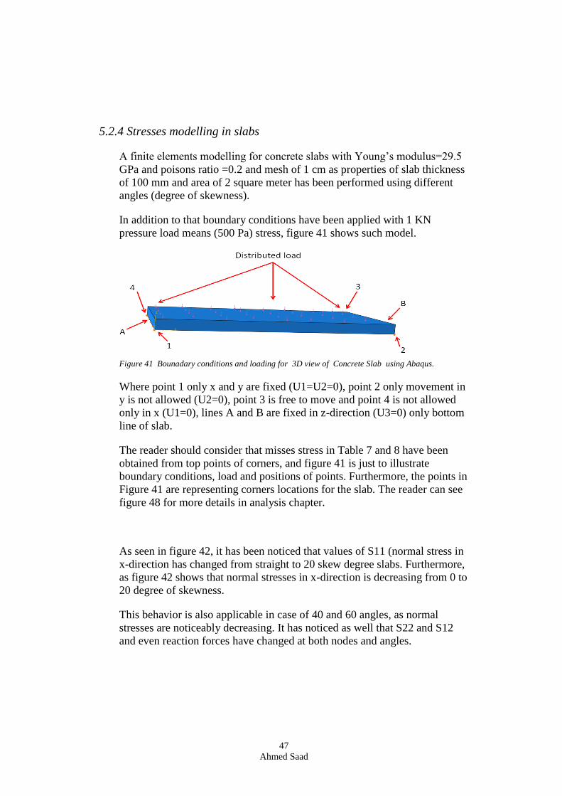
As seen in Abaqus modelling that maximum stresses were higher near edge
of specimen neck and this can be seen in figure 40 which shows normal
stresses in both directions x- axis and y-axis
Figure 40 Normal stresses in for unixial tension test a) Normal stress in x-direction b) Normal
stress in y-direction.
a) b)
47
Ahmed Saad
5.2.4 Stresses modelling in slabs
A finite elements modelling for concrete slabs with Young’s modulus=29.5
GPa and poisons ratio =0.2 and mesh of 1 cm as properties of slab thickness
of 100 mm and area of 2 square meter has been performed using different
angles (degree of skewness).
In addition to that boundary conditions have been applied with 1 KN
pressure load means (500 Pa) stress, figure 41 shows such model.
Figure 41 Bounadary conditions and loading for 3D view of Concrete Slab using Abaqus.
Where point 1 only x and y are fixed (U1=U2=0), point 2 only movement in
y is not allowed (U2=0), point 3 is free to move and point 4 is not allowed
only in x (U1=0), lines A and B are fixed in z-direction (U3=0) only bottom
line of slab.
The reader should consider that misses stress in Table 7 and 8 have been
obtained from top points of corners, and figure 41 is just to illustrate
boundary conditions, load and positions of points. Furthermore, the points in
Figure 41 are representing corners locations for the slab. The reader can see
figure 48 for more details in analysis chapter.
As seen in figure 42, it has been noticed that values of S11 (normal stress in
x-direction has changed from straight to 20 skew degree slabs. Furthermore,
as figure 42 shows that normal stresses in x-direction is decreasing from 0 to
20 degree of skewness.
This behavior is also applicable in case of 40 and 60 angles, as normal
stresses are noticeably decreasing. It has noticed as well that S22 and S12
and even reaction forces have changed at both nodes and angles.
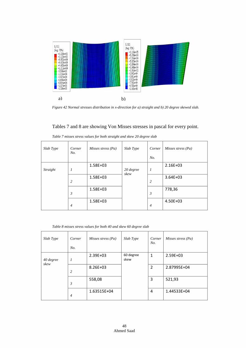
48
Ahmed Saad
Figure 42 Normal stresses distribution in x-direction for a) straight and b) 20 degree skewed slab.
Tables 7 and 8 are showing Von Misses stresses in pascal for every point.
Table 7 misses stress values for both straight and skew 20 degree slab
Slab Type Corner
No.
Misses stress (Pa) Slab Type Corner
No.
Misses stress (Pa)
Straight 1 1.58E+03
20 degree
skew
1 2.16E+03
2 1.58E+03 2
3.64E+03
3 1.58E+03 3
778,36
4 1.58E+03 4
4.50E+03
Table 8 misses stress values for both 40 and skew 60 degree slab
Slab Type Corner
No.
Misses stress (Pa) Slab Type Corner
No.
Misses stress (Pa)
40 degree
skew
1 2.39E+03
60 degree skew
1 2.59E+03
2 8.26E+03
2 2.87995E+04
3 558,08
3 521,93
4 1.63515E+04
4 1.44533E+04
a) b)
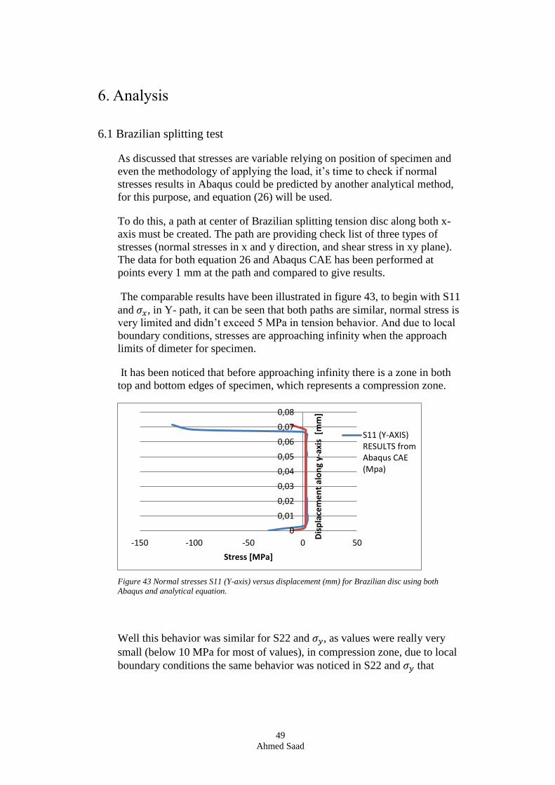
49
Ahmed Saad
6. Analysis
6.1 Brazilian splitting test
As discussed that stresses are variable relying on position of specimen and
even the methodology of applying the load, it’s time to check if normal
stresses results in Abaqus could be predicted by another analytical method,
for this purpose, and equation (26) will be used.
To do this, a path at center of Brazilian splitting tension disc along both x-
axis must be created. The path are providing check list of three types of
stresses (normal stresses in x and y direction, and shear stress in xy plane).
The data for both equation 26 and Abaqus CAE has been performed at
points every 1 mm at the path and compared to give results.
The comparable results have been illustrated in figure 43, to begin with S11
and 𝜎𝑥, in Y- path, it can be seen that both paths are similar, normal stress is
very limited and didn’t exceed 5 MPa in tension behavior. And due to local
boundary conditions, stresses are approaching infinity when the approach
limits of dimeter for specimen.
It has been noticed that before approaching infinity there is a zone in both
top and bottom edges of specimen, which represents a compression zone.
Figure 43 Normal stresses S11 (Y-axis) versus displacement (mm) for Brazilian disc using both
Abaqus and analytical equation.
Well this behavior was similar for S22 and 𝜎𝑦, as values were really very
small (below 10 MPa for most of values), in compression zone, due to local
boundary conditions the same behavior was noticed in S22 and 𝜎𝑦 that
0
0,01
0,02
0,03
0,04
0,05
0,06
0,07
0,08
-150 -100 -50 0 50
Dis
pla
cem
en
t al
on
g y-
axis
[m
m]
Stress [MPa]
S11 (Y-AXIS)RESULTS fromAbaqus CAE(Mpa)
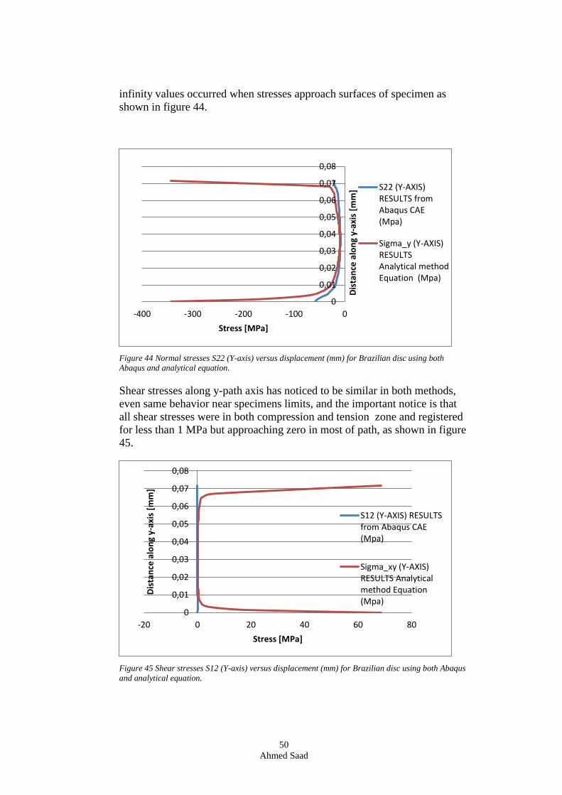
50
Ahmed Saad
infinity values occurred when stresses approach surfaces of specimen as
shown in figure 44.
Figure 44 Normal stresses S22 (Y-axis) versus displacement (mm) for Brazilian disc using both
Abaqus and analytical equation.
Shear stresses along y-path axis has noticed to be similar in both methods,
even same behavior near specimens limits, and the important notice is that
all shear stresses were in both compression and tension zone and registered
for less than 1 MPa but approaching zero in most of path, as shown in figure
45.
Figure 45 Shear stresses S12 (Y-axis) versus displacement (mm) for Brazilian disc using both Abaqus
and analytical equation.
0
0,01
0,02
0,03
0,04
0,05
0,06
0,07
0,08
-400 -300 -200 -100 0
Dis
tan
ce a
lon
g y-
axis
[m
m]
Stress [MPa]
S22 (Y-AXIS)RESULTS fromAbaqus CAE(Mpa)
Sigma_y (Y-AXIS)RESULTSAnalytical methodEquation (Mpa)
0
0,01
0,02
0,03
0,04
0,05
0,06
0,07
0,08
-20 0 20 40 60 80
Dis
tan
ce a
lon
g y-
axis
[m
m]
Stress [MPa]
S12 (Y-AXIS) RESULTSfrom Abaqus CAE(Mpa)
Sigma_xy (Y-AXIS)RESULTS Analyticalmethod Equation(Mpa)
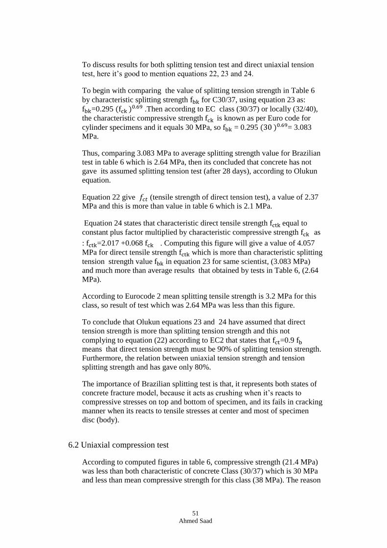
51
Ahmed Saad
To discuss results for both splitting tension test and direct uniaxial tension
test, here it’s good to mention equations 22, 23 and 24.
To begin with comparing the value of splitting tension strength in Table 6
by characteristic splitting strength fbk for C30/37, using equation 23 as:
fbk=0.295 (fck )0.69 .Then according to EC class (30/37) or locally (32/40),
the characteristic compressive strength fck is known as per Euro code for
cylinder specimens and it equals 30 MPa, so fbk = 0.295 (30 )0.69= 3.083
MPa.
Thus, comparing 3.083 MPa to average splitting strength value for Brazilian
test in table 6 which is 2.64 MPa, then its concluded that concrete has not
gave its assumed splitting tension test (after 28 days), according to Olukun
equation.
Equation 22 give 𝑓𝑐𝑡 (tensile strength of direct tension test), a value of 2.37
MPa and this is more than value in table 6 which is 2.1 MPa.
Equation 24 states that characteristic direct tensile strength fctk equal to
constant plus factor multiplied by characteristic compressive strength fck as
: fctk=2.017 +0.068 fck . Computing this figure will give a value of 4.057
MPa for direct tensile strength fctk which is more than characteristic splitting
tension strength value fbk in equation 23 for same scientist, (3.083 MPa)
and much more than average results that obtained by tests in Table 6, (2.64
MPa).
According to Eurocode 2 mean splitting tensile strength is 3.2 MPa for this
class, so result of test which was 2.64 MPa was less than this figure.
To conclude that Olukun equations 23 and 24 have assumed that direct
tension strength is more than splitting tension strength and this not
complying to equation (22) according to EC2 that states that fct=0.9 fb
means that direct tension strength must be 90% of splitting tension strength.
Furthermore, the relation between uniaxial tension strength and tension
splitting strength and has gave only 80%.
The importance of Brazilian splitting test is that, it represents both states of
concrete fracture model, because it acts as crushing when it’s reacts to
compressive stresses on top and bottom of specimen, and its fails in cracking
manner when its reacts to tensile stresses at center and most of specimen
disc (body).
6.2 Uniaxial compression test
According to computed figures in table 6, compressive strength (21.4 MPa)
was less than both characteristic of concrete Class (30/37) which is 30 MPa
and less than mean compressive strength for this class (38 MPa). The reason
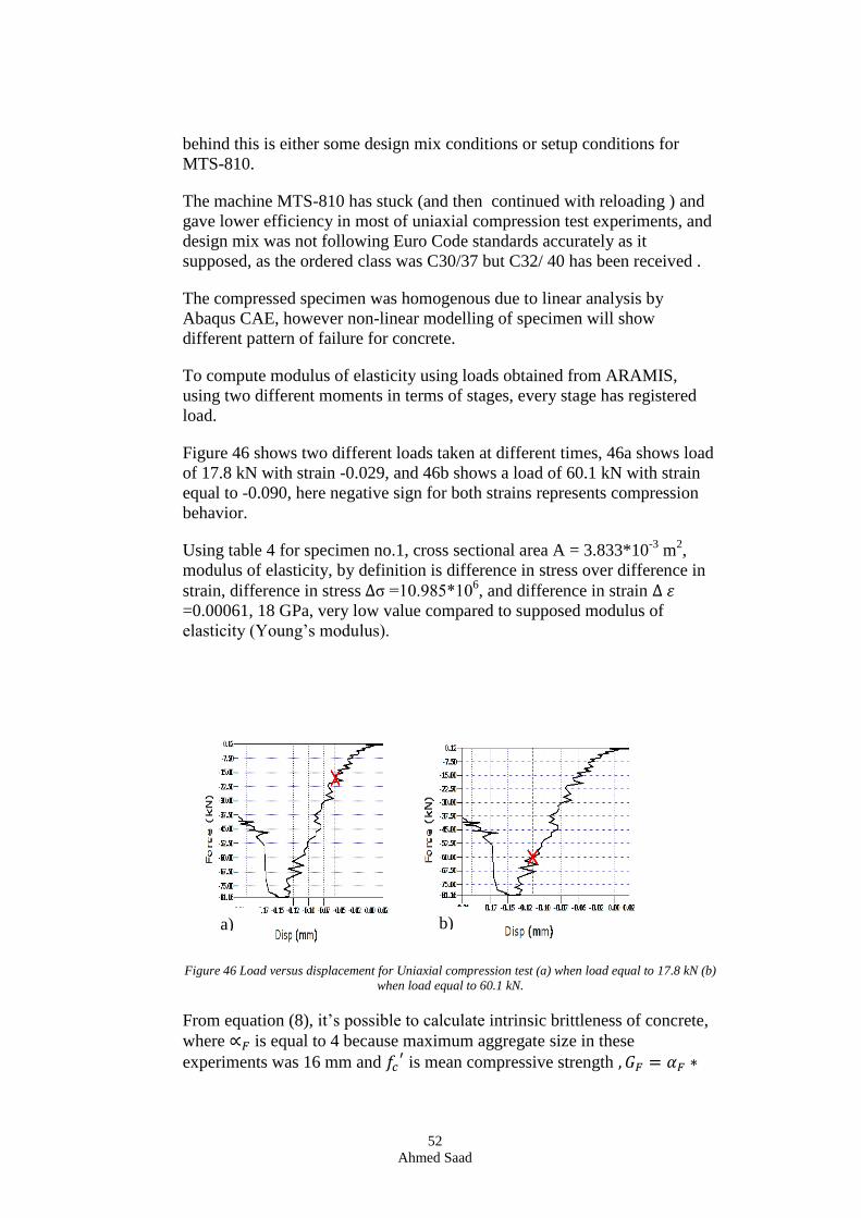
52
Ahmed Saad
behind this is either some design mix conditions or setup conditions for
MTS-810.
The machine MTS-810 has stuck (and then continued with reloading ) and
gave lower efficiency in most of uniaxial compression test experiments, and
design mix was not following Euro Code standards accurately as it
supposed, as the ordered class was C30/37 but C32/ 40 has been received .
The compressed specimen was homogenous due to linear analysis by
Abaqus CAE, however non-linear modelling of specimen will show
different pattern of failure for concrete.
To compute modulus of elasticity using loads obtained from ARAMIS,
using two different moments in terms of stages, every stage has registered
load.
Figure 46 shows two different loads taken at different times, 46a shows load
of 17.8 kN with strain -0.029, and 46b shows a load of 60.1 kN with strain
equal to -0.090, here negative sign for both strains represents compression
behavior.
Using table 4 for specimen no.1, cross sectional area A = 3.833*10-3
m2,
modulus of elasticity, by definition is difference in stress over difference in
strain, difference in stress ∆σ =10.985*106, and difference in strain ∆ 𝜀
=0.00061, 18 GPa, very low value compared to supposed modulus of
elasticity (Young’s modulus).
Figure 46 Load versus displacement for Uniaxial compression test (a) when load equal to 17.8 kN (b)
when load equal to 60.1 kN.
From equation (8), it’s possible to calculate intrinsic brittleness of concrete,
where ∝𝐹 is equal to 4 because maximum aggregate size in these
experiments was 16 mm and 𝑓𝑐′ is mean compressive strength , 𝐺𝐹 = 𝛼𝐹 ∗
a) b)
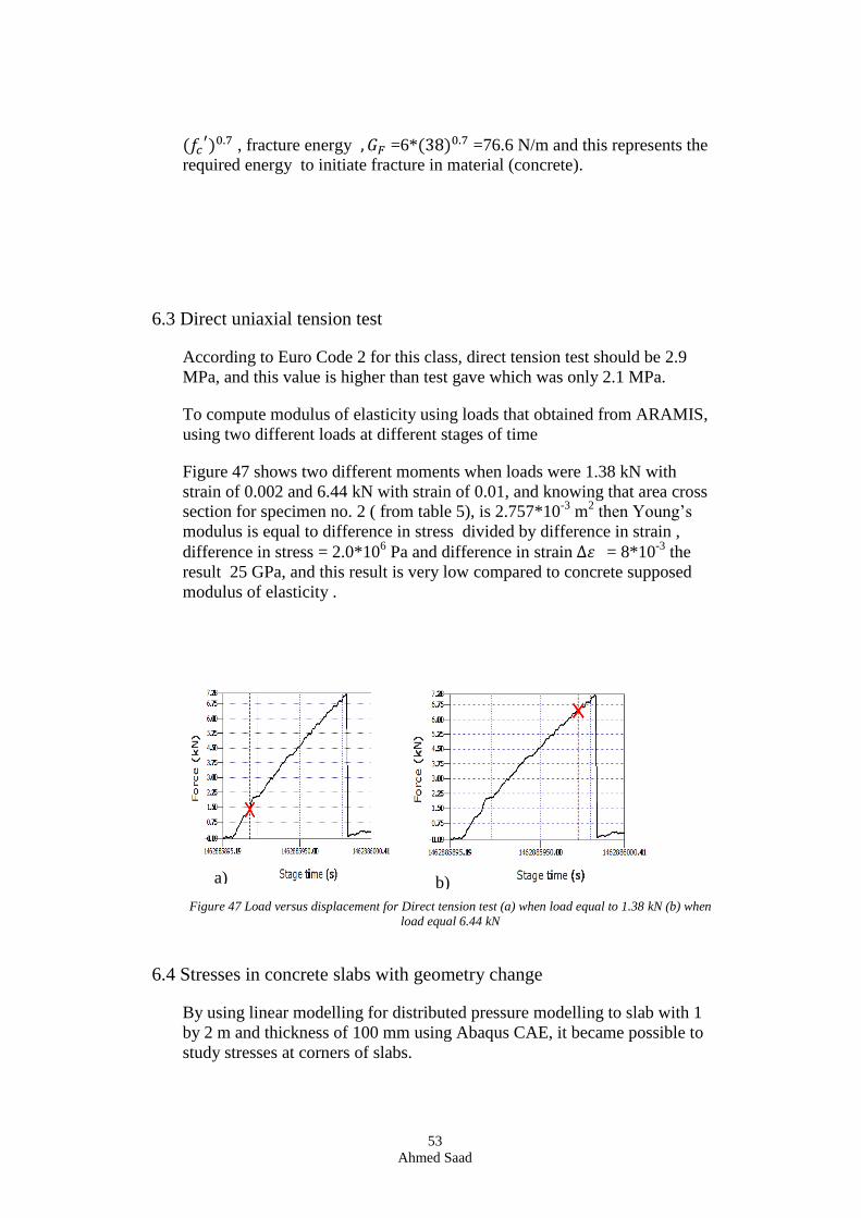
53
Ahmed Saad
(𝑓𝑐′)0.7 , fracture energy , 𝐺𝐹 =6*(38)0.7 =76.6 N/m and this represents the
required energy to initiate fracture in material (concrete).
6.3 Direct uniaxial tension test
According to Euro Code 2 for this class, direct tension test should be 2.9
MPa, and this value is higher than test gave which was only 2.1 MPa.
To compute modulus of elasticity using loads that obtained from ARAMIS,
using two different loads at different stages of time
Figure 47 shows two different moments when loads were 1.38 kN with
strain of 0.002 and 6.44 kN with strain of 0.01, and knowing that area cross
section for specimen no. 2 ( from table 5), is 2.757*10-3
m2 then Young’s
modulus is equal to difference in stress divided by difference in strain ,
difference in stress = 2.0*106 Pa and difference in strain ∆𝜀 = 8*10
-3 the
result 25 GPa, and this result is very low compared to concrete supposed
modulus of elasticity .
Figure 47 Load versus displacement for Direct tension test (a) when load equal to 1.38 kN (b) when
load equal 6.44 kN
6.4 Stresses in concrete slabs with geometry change
By using linear modelling for distributed pressure modelling to slab with 1
by 2 m and thickness of 100 mm using Abaqus CAE, it became possible to
study stresses at corners of slabs.
a) b)
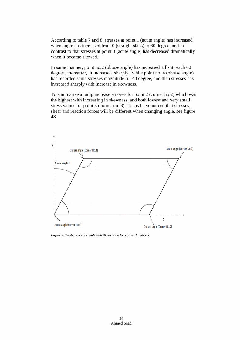
54
Ahmed Saad
According to table 7 and 8, stresses at point 1 (acute angle) has increased
when angle has increased from 0 (straight slabs) to 60 degree, and in
contrast to that stresses at point 3 (acute angle) has decreased dramatically
when it became skewed.
In same manner, point no.2 (obtuse angle) has increased tills it reach 60
degree , thereafter, it increased sharply, while point no. 4 (obtuse angle)
has recorded same stresses magnitude till 40 degree, and then stresses has
increased sharply with increase in skewness.
To summarize a jump increase stresses for point 2 (corner no.2) which was
the highest with increasing in skewness, and both lowest and very small
stress values for point 3 (corner no. 3). It has been noticed that stresses,
shear and reaction forces will be different when changing angle, see figure
48.
Figure 48 Slab plan view with with illustration for corner locations.
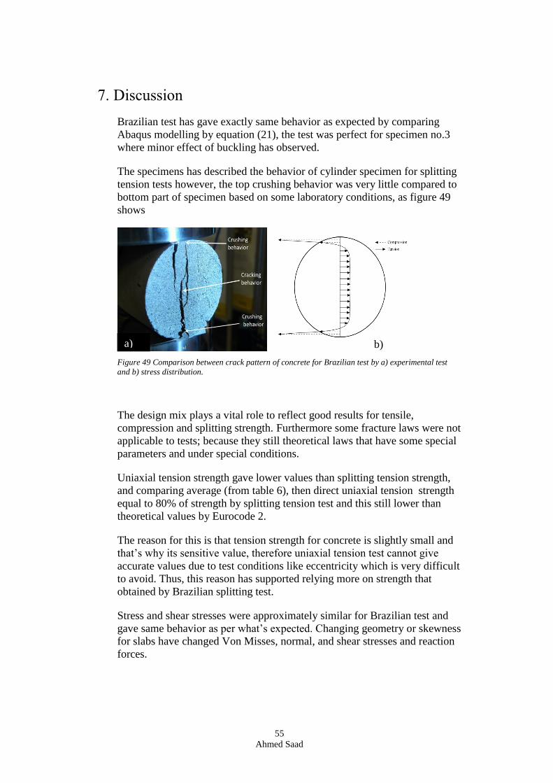
55
Ahmed Saad
7. Discussion
Brazilian test has gave exactly same behavior as expected by comparing
Abaqus modelling by equation (21), the test was perfect for specimen no.3
where minor effect of buckling has observed.
The specimens has described the behavior of cylinder specimen for splitting
tension tests however, the top crushing behavior was very little compared to
bottom part of specimen based on some laboratory conditions, as figure 49
shows
Figure 49 Comparison between crack pattern of concrete for Brazilian test by a) experimental test
and b) stress distribution.
The design mix plays a vital role to reflect good results for tensile,
compression and splitting strength. Furthermore some fracture laws were not
applicable to tests; because they still theoretical laws that have some special
parameters and under special conditions.
Uniaxial tension strength gave lower values than splitting tension strength,
and comparing average (from table 6), then direct uniaxial tension strength
equal to 80% of strength by splitting tension test and this still lower than
theoretical values by Eurocode 2.
The reason for this is that tension strength for concrete is slightly small and
that’s why its sensitive value, therefore uniaxial tension test cannot give
accurate values due to test conditions like eccentricity which is very difficult
to avoid. Thus, this reason has supported relying more on strength that
obtained by Brazilian splitting test.
Stress and shear stresses were approximately similar for Brazilian test and
gave same behavior as per what’s expected. Changing geometry or skewness
for slabs have changed Von Misses, normal, and shear stresses and reaction
forces.
a) b)
56
Ahmed Saad
8. Conclusion
It has been concluded that both laboratory conditions like loading and design
mix could change results significantly, and that’s reason behind that strength
for compression test were below than those estimated ones by theoretical
equations.
Regarding uniaxial tension and splitting tension tests, they gave similar
behavior as expected but still less than both Eurocode values (2.9 MPa for
uniaxial tensile strength and 3.2 MPa for splitting tensile strength) and
percentage of relation between them (90 % as per theory, while it was 80%
according to experimental results).
Regarding compressive strength, it gave 21.43 MPa which is less than
values according to Euro code (30 MPa for characteristic compressive
strength after 28 days, and 38 MPa for mean compressive strength after 28
days).
The calculated values for modulus of elasticity by both compression and
tension test were lower than expected 29.5 GPa. However they are near this
value, but again design mix and hardening of concrete period (28 days)
plays main factor for this variance.
Brazilian specimen no.3 has gave much realistic results because its least
affected by laboratory conditions like buckling. Brazilian test is important
because it shows both behavior of concrete, both tension and compression in
a disc. Furthermore, in Brazilian disc, cracks propagate from center to reach
ends, in addition to minor cracks that occur in different positions.
Using ARAMIS cameras, the cracks observation is possible to record. It’s
recommended to calculate final strain just before cracking, because crack
stage gives incorrect data about strains and deformations dimensions see
figure 25 and 30.
Regarding stresses in slabs, it’s proved that stress, shear and reaction forces
varies in bridges where skewness occurs. It is important to have more
research on this because the demand for road and train intersection bridges is
increasing. The slabs can be studied in
57
Ahmed Saad
9. Future work
This thesis has not dealt with non-linear behavior of concrete, nor with
modelling of steel for reinforced concrete structures. Therefore, it’s
important to do this future work. Concrete is heterogeneous nonlinear
material by its nature, therefore it’s required to model it using special
analytical methods.
Furthermore, since cracking is major source of material nonlinearity for
reinforced concrete structures, realistic models need to be developed in order
to accurately predict the load-deformation behavior of reinforced concrete
members.
Fracture mechanics for both RCC slabs and concrete slabs need more
research, and laboratory should be equipped with machines that are capable
to handle concrete and RCC slabs.
9.1 Non-linear behavior of concrete in FEM
Concrete is main constituent material in many structures. Concrete behavior
is non-linear, therefore there is an increasing demand to find the exact
solution of the problems. One way to find solution is by using computer
based method for designing and simulation such us Abaqus.
The researcher can use either of smeared or concrete damage plasticity to
simulate the model.
9.1.1 The smeared crack concrete model
This method is designed mainly to simulate reinforced concrete structures;
however it could be used to simulate plain concrete structures. It’s based on
integration of each point of finite elements rather than describing macro
cracks in concrete. It’s relying on a concept that material is exhibiting either
tensile crack or compressive crush, (Chaudhari, et al., 2012).
Therefore it’s emphasizing on crack concept and strain has both elastic and
plastic part. This model has parameters that should be taken based on
Abaqus manual and other technical resources for concrete.
9.1.2 Concrete damage plasticity
This model is based on damage, and damage in concrete as quassi-brittle
material is described as dissipated fracture energy required to generate
mirocracks. The stress-strain is determined by equation, (Chaudhari, et al.,
2012):
σ=(1-d)𝐷0𝑒𝑙 (27)

58
Ahmed Saad
σ=(1-d)𝐷0𝑒𝑙 where σ is stress , 𝐷0
𝑒𝑙 is initial elastic undamaged stiffness of
material and d is scalar stiffness degradation variable, however there are
many parameters in this model that rely on material properties and
geometry, and can be taken by Abaqus manual and other technical
resources.
59
Ahmed Saad
References
(1) Arghya Deb. size effect in concrete under compression. Department of civil
engineering. 2000, India
(2) Ausum Kar, Vikash Khatri, P.R Maiti. Skew Bridges. International Journal of
engineering research and development. Volume 2, p13-18(2013).
(3) Bhushan L. Karihaloo. Fracture mechanics & structural concrete.2001: Pearson
education, Australia
(4) Bostoncommons.net. High technology
(5) Diyuan Li and Louis Ngai Yuen Wong. The Brazilian Disc Test forRock Mechnics
Applications: Review and New Insights. Rock Mech Rock Eng., Springer-Verlag
(2012).
(6) Dr.h.c.H ,(TUW). University of Vienna.
(7) Kanhaiyra Lal Pandey, Behaviour of Reinforced concrete skew slab under
different loading conditions. GJESR Research. vol.1, p21-30 (2014).
(8) Hyo-Gyoung Kwak & FILIP C. FILIPPOU. Finite elements of Reinforced concrete
structures under monotonic loads.1990. A report on research conducted under
Grant RTA-59M848 from California Department of Transport.
(9) JoeW. Kelly.Cracks in concrete: the causes and cures.The Aberdeen group.
Publication no. c640089.(1964).
(10) Jorge Daniel Riera, Leticia Fleck Fdel Miguel, Ignacio Iturrrioz. Assesment of
Brazian tensile test by means of truss-like Discrete Element Method (DEM)
with imperfect mesh Engineering structures Jorurnal. 81, p10-21 (2014).
(11) Ibrahim S I Harba. Effect of skew angle on behavior of simply supported R.C T-
Beam Bridge Decks. Aian Research Publishing Network (ARPN) Journal of
engineering and applied sciences. Volume 6, p1-14 (2011).
(12) Jonathan S. Goode, Joe Friedrichsen, Natalie Mach; Denali Lander,
Christopher Valenti, Denise W. Carlson, and Malinda Schaefer Zarske, Strength
of Materials. Integrated Teaching and Learning Program and Laboratory,
University of Colorado Boulder, 2006.
(13) Euro code 2: Design of concrete structures, EN 1992.
(14) Ezdin Duran. Design of Edge Beams. 2014. Master of science Thesis. KTH
(university), Sweden.
(15) Helena Alferdsson & Johanna Spål. Cracking behavior of concrete subjected to
restraint forces. 2008. Master of science thesis, Chalmers University, Göteborg,
Sweden.
(16) Lucas.com.Engineering analysis and design software.
(17) Madhu Sharma. Finite element modelling of Reinforced concrete slabs. 2011.
Master of science Thesis, Thapar University. Patiala, India.
(18) Md.Khasro Miah and Ahsnal Kabir. A study on reinforced concrete skew slab
behavior. Journal of civil engineering (EIB). 33, P91-103, (2005).
60
Ahmed Saad
(19) Merhardad Bisadi, Sharizan Bahrom. A parametric study of skewed railway
bridge, Austrailian journal of basic and Applied sciences. 7(2), p 33-36 (2013).
(20) P.Banforth, D.Chisholm, J.Gibbs and T.Harrisson. Properties of concrete for use
in Eurocode 2. Cement and concrete publication, P1-53, (2000).
(21) Sindhu B.V., Ashwin K.N, Dattart reya J.K., SV Dinesh, effect of skew angle on
static beahviour or reinforced concrete slab bridge decks. International Journal
of Research in engineering and Technology. P50-58 (2013).
(22) S.V. Chaudhari and M.A Chakrabrti.Modelling of concrete for nonlinear
analysis using Finite element code Abaqus.Interanational Journal of computer
.Volume 44 No.7,April (2012).
(23) Théoret, P., Massicotte, B., and Conciatori, D. Analysis and design of straight
and skewed slab bridges. Journal of bridge Engineering, 17(2). P289-301(2012).
(24) Viktor Ansnaes and Hisham Elgazzar. Concrete cracks in composite bridges.
2012: Master of Science Thesis. KTH (university), Sweden.
(25) Y-H. Lee, K. William and H-D Kang. Experimental observations of concrete
behavior under uniaxial compression. Fracture mechanics of concrete
structures AEDIFICATO publishers.(1995).
(26) Zenzile Brooks, Fracture process zone. Microstructure and Nano mechanics in
Quasi-Brittle Materials. 2013: PhD Thesis. Massachusetts Institute of
Technology (MIT), USA.

61
Ahmed Saad
Appendixes
Appendix 1: Pictures for test setup.
Appendix 2: Design mix recipe.
Appendix 3: Failure pattern for specimens
Appendix 4: ARAMIS cameras photos for Brazilian test
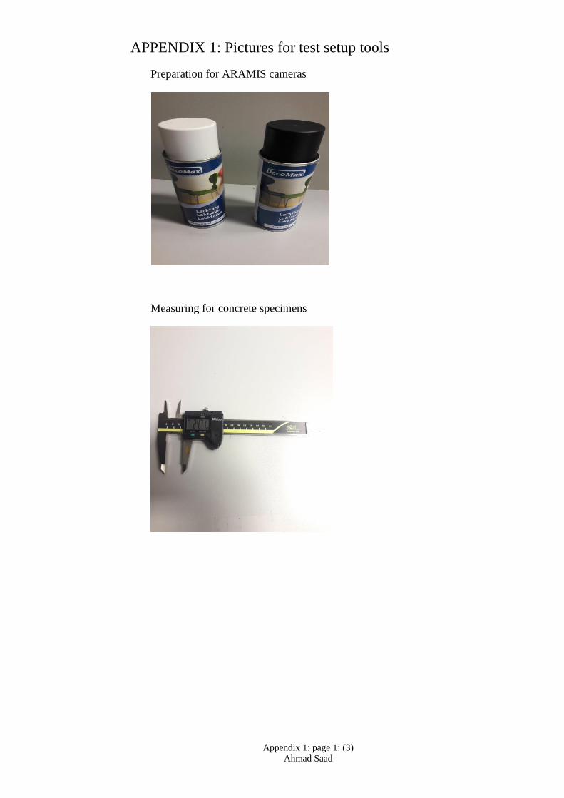
Appendix 1: page 1: (3)
Ahmad Saad
APPENDIX 1: Pictures for test setup tools
Preparation for ARAMIS cameras
Measuring for concrete specimens
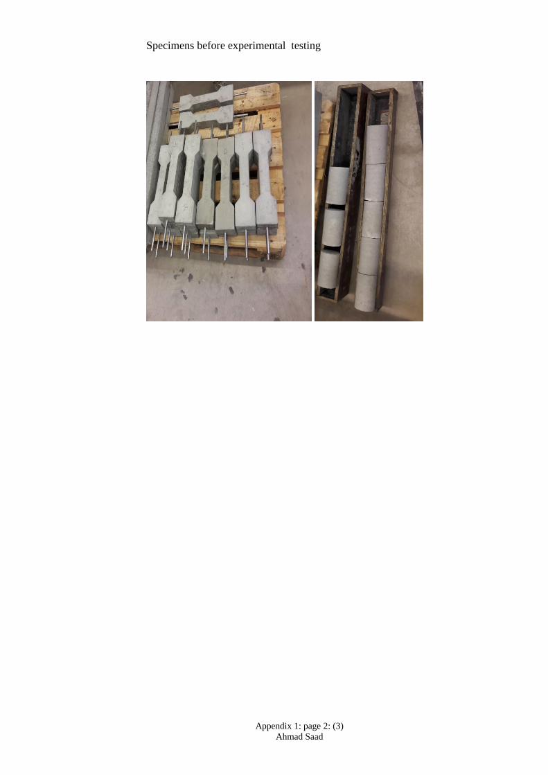
Appendix 1: page 2: (3)
Ahmad Saad
Specimens before experimental testing
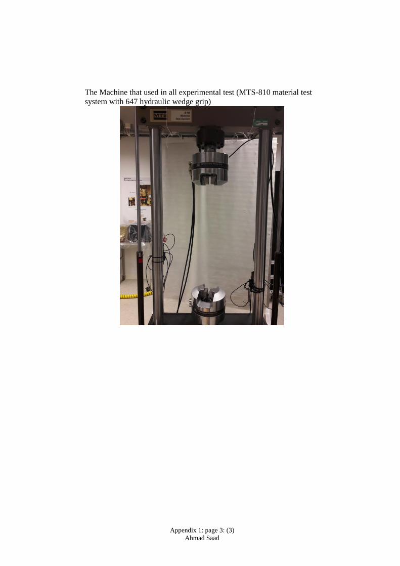
Appendix 1: page 3: (3)
Ahmad Saad
The Machine that used in all experimental test (MTS-810 material test
system with 647 hydraulic wedge grip)
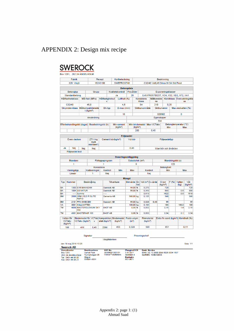
Appendix 2: page 1: (1)
Ahmad Saad
APPENDIX 2: Design mix recipe
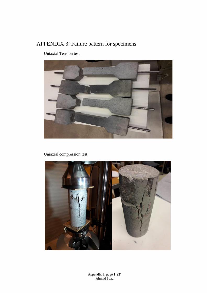
Appendix 3: page 1: (2)
Ahmad Saad
APPENDIX 3: Failure pattern for specimens
Uniaxial Tension test
Uniaxial compression test
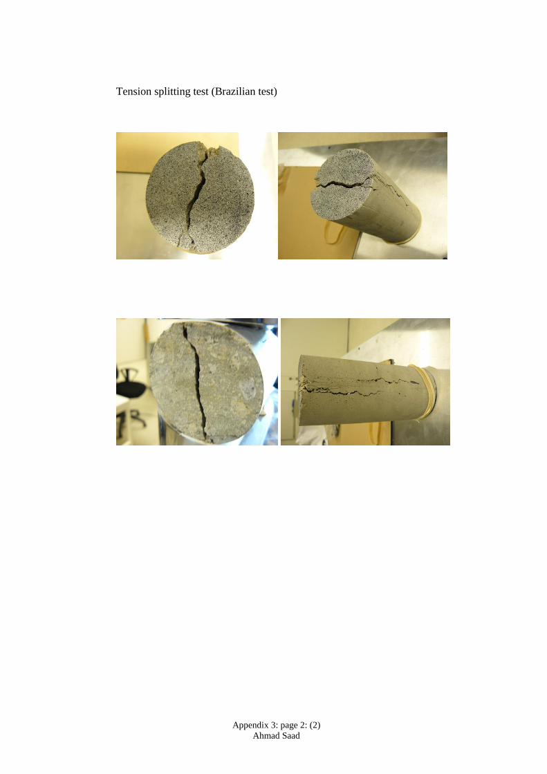
Appendix 3: page 2: (2)
Ahmad Saad
Tension splitting test (Brazilian test)
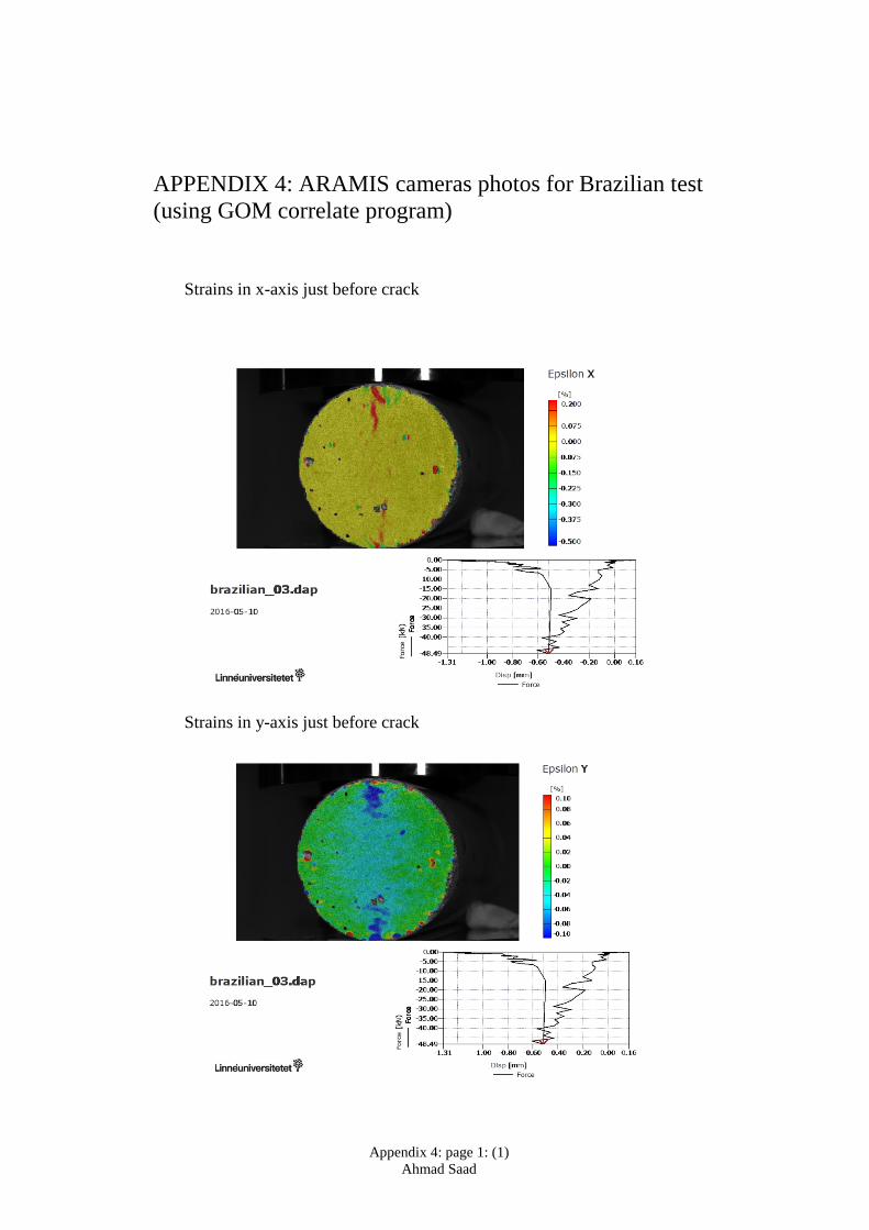
Appendix 4: page 1: (1)
Ahmad Saad
APPENDIX 4: ARAMIS cameras photos for Brazilian test
(using GOM correlate program)
Strains in x-axis just before crack
Strains in y-axis just before crack

Faculty of Technology 351 95 Växjö, Sweden Telephone: +46 772-28 80 00, fax +46 470-832 17
Recommended