August 2013
FORECLOSURES AND LOCAL GOVERNMENT REVENUES FROM THE PROPERTY TAX: THE CASE OF GEORGIA SCHOOL DISTRICTS
James Alm*Tulane University
Robert D. BuschmanGeorgia State University
David L. SjoquistGeorgia State University
ABSTRACT Historically, local governments in the United States have relied on the property tax as one of their main sources of own-source revenues. With the recent collapse of housing prices and the resulting increase in foreclosures, many observers have speculated that the local governments will suffer significant revenue losses, either immediately or in the near future. However, to our knowledge there is no existing work that examines the impacts of foreclosures on property values and the subsequent impacts on property tax revenues. We use recently available proprietary information from RealtyTrac on annual foreclosure “activity” (e.g., the flow of newly foreclosed properties into foreclosure filings), for the period 2006 through 2011, merged with information on local government revenues and economic data, to estimate the impacts of foreclosures on local government property tax revenues, as well as on market values and property tax levies. We focus on school districts in the State of Georgia, and address the question: How have recent foreclosures affected the property tax system of local governments? Across various specifications, we find that foreclosure activity had significant impacts on property tax bases, levies, and revenues.
JEL CLASSIFICATIONS: H2, H7, R3, R5.
KEYWORDS: property tax; local government finance; assessment; tax base elasticity.
* Corresponding author: James Alm, Department of Economics, Tulane University, 208 Tilton Hall, 6823 St. Charles Avenue, New Orleans, LA 70118 (phone 1 504 862 8344; fax 1 504 865 5869). Email addresses: [email protected] (Alm); [email protected] (Buschman); [email protected] (Sjoquist). We thank the Lincoln Institute of Land Policy for financial support, Andrew Hanson for comments on an earlier version of the paper, Lakshmi Pandey for preparing the maps, and Jim Martin for assistance in understanding the foreclosure process.
1

I. INTRODUCTION
Historically, local governments in the United States have relied on the property tax as one of
their main sources of own-source revenues. With the collapse of housing prices and the resulting
increase in foreclosures that followed the “Great Recession”, many observers speculated that local
governments would suffer significant revenue losses, either immediately or in the near future.
However, the actual impact of foreclosures on property tax revenues is, surprisingly, unknown at
present. While there are several studies of the effect of foreclosures on value of foreclosed property
and its immediate surrounding properties, to our knowledge there is no existing work that examines
the impacts of foreclosures on property tax revenues. Our purpose in this paper is to explore the effect
of foreclosures on the property tax base, levy, and revenue.
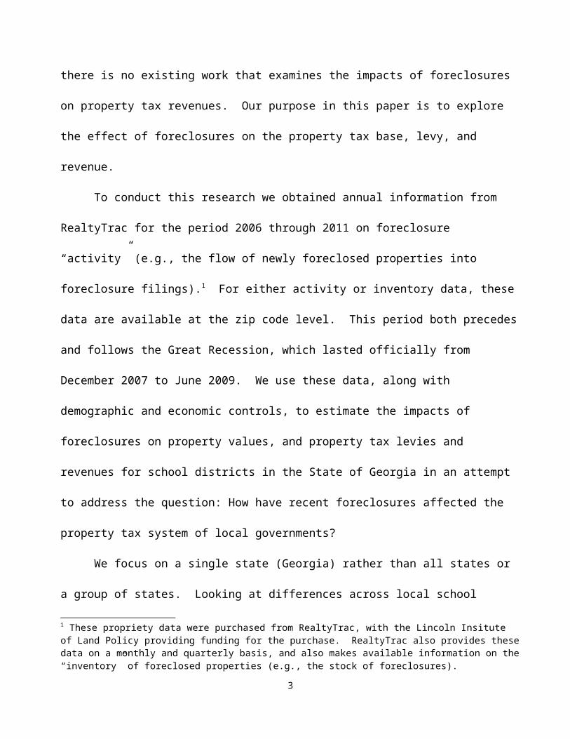
To conduct this research we obtained annual information from RealtyTrac for the period 2006
through 2011 on foreclosure “activity” (e.g., the flow of newly foreclosed properties into foreclosure
filings).1 For either activity or inventory data, these data are available at the zip code level. This
period both precedes and follows the Great Recession, which lasted officially from December 2007 to
June 2009. We use these data, along with demographic and economic controls, to estimate the
impacts of foreclosures on property values, and property tax levies and revenues for school districts in
the State of Georgia in an attempt to address the question: How have recent foreclosures affected the
property tax system of local governments?
We focus on a single state (Georgia) rather than all states or a group of states. Looking at
differences across local school systems within a single state has some advantages over considering
differences across states. By focusing on a single state, we need not consider how to control for the
many ways in which institutional factors may differ across states. Georgia is also a good state to use
1 These propriety data were purchased from RealtyTrac, with the Lincoln Insitute of Land Policy providing funding for the purchase. RealtyTrac also provides these data on a monthly and quarterly basis, and also makes available information on the “inventory” of foreclosed properties (e.g., the stock of foreclosures).
2
to study the effects of the Great Recession and its impact on foreclosures. Georgia is in many ways
roughly an “average” state. For example, Georgia’s median household income in 2006 was $46,832,
ranking it 24th in the U.S.; local share of funding for K-12 in 2006 was 47.8 percent in Georgia
compared to 43.7 percent for the U.S.; in 2006, property tax revene as a share of state and local tax
revenue was 28.7 percent for Georgia and 30.8 percent for the U.S. Of some note, Georgia was hit
hard by the Great Recession; Georgia’s unemployment rate went from 4.7 percent in 2006 to 10.2
percent in 2010 while the U.S. unemployment rate went from 4.6 percent to 9.6 percent.
We examine detailed information on property tax assessments and property tax rates for local
school districts in the State of Georgia, focusing on the impact of foreclosures (and other factors) on
the property tax base, levy, and revenue. Our empirical analysis indicates that larger increases in
personal income per capita, in population, and in employment all positively and statistically
significantly affect the percentage change in the tax base; importantly, our results also show
significant negative effects of foreclosures. We also estimate regressions to see whether foreclosure
activity affects the property tax levy and property tax revenues, with other factors (e.g., income,
population, and employment growth) held constant. Again, we find that foreclosure activity has
significant impacts; for example, a rise in foreclosures is associated with a reduction in the levy, and
foreclosures also have a negative impact on revenues, after controlling for changes in the base and
other factors. Overall, we find that foreclosure activity had significant impacts on the property tax
base, on property tax levies, and on property tax revenues.
II. HOUSING PRICES, FORECLOSURES, AND SCHOOL DISTRICT PROPERTY TAX REVENUES
Local governments in the United States typically rely on several sources of own-source
revenues, including individual income taxes, general sales taxes, specific excise taxes, fees and
3

charges, and local property taxes. Of these, the dominant source is by far the property tax. In 2011,
local property taxes accounted for roughly three-fourths of total local government tax revenues and for
nearly one-half of total local own-source revenues (including fees and charges).2
The Great Recession had serious and negative effects on the level of economic activity, and
these effects have in turn depressed tax revenues, especially for taxes whose bases vary closely with
economic activity, like income and sales taxes (Anderson, 2010; Mikesell and Mullins, 2010; Boyd,
2010). However, an important feature of the property tax is that its base (i.e., assessed value) does not
automatically change over time since, in the absence of a formal and deliberate change in assessment,
any change in the market value of housing does not necessarily translate into a change in assessed
value. Lags in these re-assessments, combined with caps on the amount by which assessed values can
be changed in any given year and with deliberate changes in millage rates, mean that changes in the
overall level of economic activity that may affect housing values may not actually affect property tax
revenues in any immediate or obvious way.3
There are several channels by which changes in the housing market, together with changes in
economic activity that accompany these housing market factors, may affect local government tax
revenues (Lutz, Molloy, and Shan, 2011). The most obvious is of course via the property tax,. Other
channels are more closely linked to economic activity. Real estate transfer taxes depend upon the
volume and the value of real estate transactions, although these taxes are of relatively little
importance. Less direct channels include those affected by declines in housing values. For example,
a decline in market housing market may depress new housing construction, thereby reducing sales tax
revenues generated by the materials used in construction and by the furnishing for a new home. The
decline in home construction and the resulting fall in employment may also reduce income taxes.
2 See http://www.census.gov/govs/estimate.3 The assessment process is analyzed in detail by Diaz (1990), Quan and Quigley (1991), Wolverton and Gallimore (1999), and McAllister et al. (2003).
4
Finally, a decline in housing values may reduce consumer expenditures (and so sales tax revenues) via
wealth effects.4
As a general framework in which these channels might be modeled, consider a simple setting.
Suppose a local jurisdiction has multiple tax sources, each generating revenues defined as the product
of a tax rate t and a tax base B. Denoting each tax source with a subscript i, then total revenues R
equal R=∑i ti Bi. Suppose now that either the tax rate or the tax base of each tax changes. Then the
percentage change in tax revenues equals:
ΔR/R = ∑i si [ΔBi/Bi + Δti/ti];
that is, the percentage change in tax revenues equals the share si of each tax in total revenues times the
sum of the percentage change in the tax base plus the percentage change in the tax rate for each of the
i taxes. A tax that has a small share of total revenues obviously has a smaller impact on changes in
revenues, even if its base and/or rate change significantly; conversely, a tax (like the local property
tax) that is a major source of revenues can have a large impact on revenues even if its base and/or rate
change by small amounts. Suppose, finally, that the tax base of each tax is some function of the level
of economic activity, denoted Y. With a change in the level of economic activity, the percentage
change in any tax base due to a changed economic environment can be written as ΔBi/Bi=εi(ΔY/Y),
where εi is the elasticity of tax base i with respect to the level of economic activity. The percentage
change in total revenues now becomes:
ΔR/R = ∑i si [ΔBi/Bi + εi (ΔY/Y) + Δti/ti],
where ΔBi/Bi now represents the deliberate administrative or policy change in the tax base of tax i,
Δti/ti represent the administrative change in tax rate i, and εi(ΔY/Y) denotes the (automatic) change in
the tax base of tax i stemming from its link with economic activity. This equation summarizes the
4 For empirical estimates of these wealth effects, see Attanasio et al. (2009), Bostic, Gabriel, and Painter (2009), and Campbell and Cocco (2007).
5
various channels by which revenues – whether of a single tax or a collection of taxes – are affected by
a change in policy actions or in external circumstances. Revenues can change if the tax rate(s) or the
tax base(s) changes; revenues can also change if the level of economic activity changes, provided that
the tax base(s) is linked in some way to economic activity, as measured by εi. If the tax base cannot
change, either because it is not responsive to economic activity, because it requires a deliberate but
unforthcoming policy action, or because it is administratively constrained, then the only remaining
source of a change in revenues is from a change in the tax rate(s).
We seek to estimate the effect of foreclosures on property tax revenue. The likely link
between foreclosures and property tax revenue in a geographic area runs as follows, as suggested by
the above framework: foreclosures decrease market values of the foreclosured houses and also of
nearby homes in the community; these decreases in housing prices get translated into decreases in
assessed value through the assessment process; decreases in assessed value may result in government
decisions to increase the property tax rate; finally, foreclosures could result in reduced collection rates.
The result could be either a net decrease or no change in property tax revenue.
We assume that property values do not immediately revert to their pre-foreclosure level at the
time the foreclosed property is returned to the private market. In addition, a new foreclosure in one
period is not necessarily returned to the private market in that period. An accumulation of foreclosed
properties that have not yet been resold by lenders to new homeowners may continue to depress prices
in the area in subsequent periods. Thus, the effect of a foreclosure in one period will likely extend
into future periods. There are several papers that estimate the effect of forclosures on individual
house values; see Frame (2010) for a survey. Typical of the effect of a foreclosure on the house value
are the findings of Campbell, Giglio, and Pathak (2011), who show that a foreclosure reduces the
home value by 22 percent; similar effects have been found by Shilling, Benjamin, and Sirmans (1990)
6
and, more recently, by Pennington-Cross (2006). Studies have also found that foreclosures reduce the
value of neighboring homes but that the effect is small and is contained within a short distance of the
foreclosure. For example, Immergluck and Smith (2006) find that property price declines about 1.0
percent as a result of a foreclosure within one-eighth of a mile, and by about 0.15 percent for a
foreclosure between one-eighth and one-quarter of a mile away; see also Leonard and Murdoch
(2009), Lin, Rosenblatt, and Yao (2009), and Campbell, Giglio, and Pathak (2011)
The link between the change in housing value and assessed value has been explored by Lutz
(2008), who estimates that it generally takes about three years for changes in housing prices to feed
through in any significant way to property tax revenues. His empirical results suggest a long-run
elasticity of property tax revenue with respect to home prices of only 0.4, in part because it takes time
for local officials to adjust assessed values to market values and in part because local officials
generally reduce millage rates in response to increases in housing prices. He also finds asymmetric
responses of property tax revenues to increases versus decreases in home prices. Relatedly, Lutz,
Molloy, and Shan (2011) present evidence that the non-property tax channels have been of relatively
little importance in their effects on state and local government revenues, either in the housing market
boom/bubble of the early-to-mid-2000s or in the more recent collapse of housing prices during the
Great Recession.
Doerner and Ihlanfeldt (2011) focus more directly on the effects of house prices on local
government revenues, using detailed panel data on Florida home prices during the 2000s. They
conclude that changes in the real price of Florida single-family housing have an asymmetric effect on
government revenues: housing price increases do not raise real per capita property tax revenues, but
decreases tend to dampen revenues. Like Lutz (2008), they conclude that these asymmetric responses
are due largely to lags between changes (positive or negative) in market prices and assessed values, to
7
caps on assessment increases, and to decreases in millage rates in response to increases in home
prices. They also find that the indirect links between home prices and local government revenues
(e.g., real estate transfer taxes, sales tax revenues on home construction materials, income taxes on
construction-related employment, wealth effects from home values on sales tax revenues) are
generally small, with the exception of an additional channel via impact fees, which are of some
importance for many Florida local governments and which are affected in significant ways by changes
in home prices. There is some other recent work that focuses more specifically on the effects of
property tax limitations on local government revenues, but this is not directly relevant to the current
research.5
Alm, Buschman, and Sjoquist (2011) document the overall trends in property tax revenues in
the United States from 1998 through 2009, and they find substantial regional and local variation.
Their data indicate that local governments, on average, seem to have avoided the significant and
negative budgetary impacts seen most clearly for state and federal governments, at least through 2009.
Alm, Buschman, and Sjoquist (2009) examine the effect of economic conditions on education
expenditures for the 1990-2006 period, a period that covers two recessions. In related work, Alm and
Sjoquist (2009) examine the the impact of economic factors on Georgia school system finances for the
1998-2009 period, using detailed information on property tax assessments and property tax rates, and
show the relevance of economic factors (including state responses to local school district conditions).
However, the last year for their data (or 2009) reflected only the very start of the housing crisis
associated with the Great Recession.
5 There is a large literature on the effects of tax limitations. For useful general discussions, see Preston and Ichniowski (1991), O’Sullivan, Sexton, and Sheffrin (1995), Dye and McGuire (1997), and Haveman and Sexton (2008). The entire issue of Public Budgeting & Finance (Volume 24, Number 2, December 2004, “Tax and Expenditure Limitations: A Quarter Century after Proposition 13”) is devoted to tax limitations.
8

Importantly, none of these studies examine the impact of foreclosures per se on property tax
revenues. The next section discusses the foreclosure process in Georgia, and the following sections
present our data, our approach for examining this issue, and our results.
III. FORECLOSURE PROCESS IN GEORGIA
To understand how foreclosures have affected the property tax system of Georgia local
governments, it is important to understand first how the foreclosure process works in the state.
Alexander (2011) provides details of this process in Georgia, and his discussion provides the basis for
the following summary.
Georgia is a non-judicial (power-of-sale) foreclosure state, and only in rare cases involving
special situations are judicial foreclosures conducted in Georgia. The ability to conduct a power-of-
sale foreclosure is determined by the expressed terms of the debt instrument, and thus language
allowing this foreclosure process is included in the mortgage instruments. If the property is a
residence, then Georgia law requires that the creditor give notice to the current owner, by certified
mail, of the intent to foreclose, and to do so at least 30 days prior to the published date of the
foreclosure sale. The creditor must advertise the proposed foreclosure sale weekly for four weeks in
the appropriate legal organ. The sale is then held on the first Tuesday of the month on the court house
steps. Unlike some states, there is no requirement of a judicial confirmation of a foreclosure sale, and
there is also no statutory right to redemption on the part of the debtor. Thus, foreclosures can be
completed in about 6 weeks. A recent 2009 federal law provides that the tenant (i.e., the owner who
has been foreclosed) can retain possession of the property, but the possession can be terminated by
giving a 90-day notice to vacate the premises.
9

The overwhelming majority of foreclosure sales are made to the creditor, who is required to
act in “good faith”. The sales price does not have to be the fair market value, but the Georgia
Supreme Ccourt has ruled that it cannot be “grossly inadequate”. If the sales price is less than the
indebtedness, the creditor can seek judicial confirmation of the foreclosure sale in order to get a
money judgment against the property owner. In a judicial confirmation of a foreclosure sale, the
creditor is required to establish the fair market value of the property in order to get a judgment for the
balance due the creditor. The proceeds of the foreclosure sale are first distributed to cover the costs
and fees of the foreclosure and to satisfy the mortgage debt. Any remaining surplus is distributed to
the debtor.
IV. DATA
Data used in this paper are taken from several sources. To measure foreclosure activity, we
use proprietary data from RealtyTrac covering the period 2006 through 2011. RealtyTrac reports
foreclosure “activity” in terms of foreclosure legal filings and notices on a zip code basis. We
measure foreclosure activity using RealtyTrac’s “notice of trustee sale” counts for each year,
aggregating zip code observations into the corresponding counties.6
We obtained from the Georgia Department of Revenue the annual property tax base (referred
to as “Net Digest” in Georgia) for each of the 180 school districts in Georgia for 1997 through 2011,
extending two years beyond the official end of the Great Recession.7 We also calculated property tax
levies for all school districts for the same periods using the net digest and reported millage rates
obtained from the Georgia Department of Revenue. The tax base is as of January 1st of the respective
year. The millage rate and resulting levy are set in the spring with tax bills being paid in the fall, the
6 Foreclosure data for zip codes that cross county lines are allocated to the particular counties in proportion to the numbers of owner-occupied housing units in the zip code that are located in each county.7 Note that of the 180 Georgia schools systems 159 are county systems, while the rest are city systems.
10
revenue from which would be reported in the following fiscal year. School districts are on a July 1st to
June 30th fiscal year, and thus (say) the 2009 tax base and levies would be reflected in revenues for
fiscal year (or school year) 2010. We use data from the Georgia Department of Education on property
tax operating revenues (referred to as maintenance and operations, or M&O, revenues) for school
districts over the same period.8 Because income, population and employment variables used in our
regressions are on a county level, digest and revenue variables for city school districts are added to
those for the county school systems in the same counties to obtain countywide totals.9 Table 1
contains descriptive statistics for these variables.
Georgia is broadly similar to other states in the local government practice of and reliance upon
property taxation, although there are some distinctive Georgia features. Property tax assessment is
conducted only by county governments in Georgia. Property tax bases are all evaluated by the state
every year, comparing actual sales of improved parcels during the year to assessed values to determine
if they are at the appropriate assessment level relative to fair market value, which is legally set at 40
percent.10 The resulting “sales ratio studies” report an “adjusted 100% digest” figure for each school
district in the state, along with the calculated ratio. We use these adjusted digest data, covering the
periods 2000 through 2011, as a measure of the market value of property in the jurisdiction.
Georgia has very few institutional property tax limitations. School district boards can
generally set their property tax millage rates without voter approval, provided that the property tax
rate for county school districts, but not city school districts, cannot exceed 20 mills without voter
approval.11 Also, there is no general assessment limitation, although one county has an assessment
8 See Rubenstein and Sjoquist (2003) for a detailed discussion of the Georgia school finance system.9 Five city school systems operate in two counties each, but digest and levy data are reported separately by county. Revenues are allocated to the counties in proportion to the levy.10 If the actual assessment ratio is not between 36 and 44 percent of fair market value, then a penalty of $5 per parcel is imposed. If the ratio is less than 36 percent, then the county is also required to pay the difference between the actual property tax revenue that the state collects from its 0.25 mill property tax rate and the level that the state would have collected if the digest had been assessed at 40 percent.11 This cap is currently binding on only 5 school systems.
11

freeze on homesteaded property. Note that in 2009 the State of Georgia imposed a temporary freeze
on assessments across the state, potentially affecting property tax revenue only in school year/fiscal
year 2010. However, with net and adjusted digests declining on a per capita basis for most counties in
2009 through 2011, it is not likely that the freeze has had a material negative effect on assessments.
Figures 1 and 2 show the distributions of annual changes, respectively, in per capita net digest and per
capita adjusted 100% digest across the 159 counties from 2001 through 2011. (Note that the bar in the
box represents the median and the box captures the observations in the 2nd and 3rd quartile.)
State and local school districts contribute about equal amounts of revenue for K-12 education.
The bulk of the grant to local districts is through a foundation program; the state has a small
equalization grant program as well.12 There were no changes in the nature of the funding formula
during the period of our analysis.
Figure 3 shows local revenue per full time equivalent (FTE) student and property taxes per
FTE in Georgia over the period 2001 through 2011 for the maintenance and operation (M&O) budget
for all local school systems. Note first that, for the M&O budget in 2011, property taxes accounted
for about 96 percent of total local school revenues and 98 percent of all property taxes collected by
local school systems. This is the highest portion of total local source revenues over the last decade;
for 2009 and 2006, property taxes accounted for about 93 percent of the total, and property taxes
accounted for 91 percent in 2001. Although property taxes per FTE peaked in 2009 along with the
total, the decline in other local revenues (e.g. local option sales taxes) has been sharper, or a 10.9
percent real decline for property taxes compared to an 11.1 percent real decline in overall revenue.13
There is considerable variation across the school systems in the annual changes in property tax
revenues. Figure 4 depicts the distribution of nominal changes by county in total M&O property tax
12 For a detailed description of Georgia school funding program, see Rubenstein and Sjoquist (2003).13 There are 10 school systems that are allowed to use a local sales tax to fund current operations. Most school systems levy a 1 percent sales tax, but the revenue can only be used for capital expenditures.
12

revenues since 2001. Even in the latest three years of declining property values, about half or more of
counties each year realized positive nominal growth in property tax revenue.
Table 2 provides some basic summary statistics on foreclosures by zip code, where
foreclosures are measured by the number of properties put up for public auction (i.e., those properties
subject to a notice of trustee sale). There are 982 zip codes in Georgia, although only 733 have
positive populations according to the Census Bureau. While RealtyTrac reports positive foreclosures
in a handful of zip codes with no reported population, we ignore these zip codes. Total foreclosures
almost doubled between 2006 and 2010, before declining in 2011. The mean number of foreclosures
is much larger than the median, implying that the distribution is highly skewed. The distribution of
foreclosures per capita is also skewed, but not as pronounced.
Table 3 shows the distribution of the number of Georgia zip codes by the number of years that
the zip code had non-zero foreclosures. Over 65 percent of the zip codes had foreclosures in each of
the 6 years, while only 7 percent had no foreclosures in all 6 years.
Figures 5 and 6 show the distribution each year of foreclosures per 100 housing units and per
1000 population, respectively, in each of Georgia’s 159 counties. The median number of foreclosures
by county increased from 0.17 per 100 housing units in 2006 to 1.18 per 100 units in 2010, more than
a six-fold increase in the median. Relative to population, the increase was of roughly the same
magnitude, from a median of 0.74 per 1000 population to 5.26.
There is a high positive correlation between foreclosure activity in 2006 and 2011 across the
counties. This correlation is 0.78 when foreclosures are measured relative to housing units and 0.74
when they are measured on a per capita basis, indicating that counties with above (below) average
foreclosure activity before the housing crisis remained above (below) average at its peak. Figure 7
presents a scatter diagram of foreclosures per 100 housing units by county in 2006 and 2010, and
13

shows that the increase in foreclosures from 2006 to 2010 was common to all counties as all points are
above the 45 degree line, albeit only slightly in a few cases.
Map 1 shows the distribution of total foreclosures by zip code across the state for the period
2006 to 2011. (Since there is a high correlation across years in the number of foreclosures, the maps
for each individual year are quite similar.) Because zip codes differ in size and housing density, we
also map the number of foreclosures per owner occupied housing unit using housing units for 2010 in
Map 2. Using housing units for 2010 will tend to understate the number of owner occupied housing
units that could be subject to foreclosure since foreclosures prior to 2010 will likely have reduced the
number of owner occupied housing units. Unfortunately, data on owner occupied housing units are
not available for intercensal years. Note that zip codes marked in white either have no foreclosures or
are missing the foreclosure data.14
As one would expect, urban and suburban counties (particularly in the Atlanta metropolitan
area) have the most foreclosures on an absolute basis. However, there are large numbers of
foreclosures in many of the less urban zip codes as well. While there is some difference in the
geographic distribution of total foreclosures and foreclosures per owner occupied housing unit, the
pattern of greater foreclosure activity in the urban and suburban areas is similar under either measure.
V. REGRESSION ANALYSIS
As noted above, property tax revenue will be affected by changes in market value, the
translation of changes in market value to taxable value, and changes in the property tax rate. To
understand the effect of the recent rise in foreclosure activity on local government revenues from the
property tax, we estimate regressions with different dependent variables related to possible channels
14 For example, an airport might have its own zip code. However, these zip codes are not likely to be visible on the map.
14
through which an effect might occur. Because of the years differ for which the various data elements
are available, the period used for various regressions also differs.
As we argued earlier, one channel is that foreclosed properties tend to sell at discounted prices,
and studies suggest that foreclosures have spillover effects on the market values of other properties in
the jurisdiction. However, changes in market values are driven by general economic conditions as
well as by foreclosures, which are also driven in part by the same general economic conditions. Thus,
we estimate regressions of the adjusted 100% digest (as a proxy for market values) on county-level
per capita income and population, both in terms of year-to-year percent changes and lagged one year
to correspond to the beginning of the fiscal year, as well as on lagged measures of foreclosure
activity.15 To account for the likelihood that foreclosure activity and market values are jointly affected
by the local severity of the recent recession, we also include a measure of the local labor market in
some regressions; specifically, we include the lagged percent change in the number of persons
employed.16 Results of these regressions are presented in Table 4.
The regression in the first column of Table 4 is a pooled regression with panel-corrected
standard errors (PCSE), while the other 6 regressions are fixed effects regressions with cluster-robust
standard errors (FE). The first three columns of results in Table 4 use data for the period 2000 to 2011
and do not include foreclosures. As expected, larger increases in personal income per capita,
population, and employment are all positively and statistically significantly affect the percentage
change in the 100% digest.
The regressions in columns 4 and 5 of Table 4 use foreclosures per housing unit, lagged one
and two years, while those in columns 6 and 7 use foreclosures relative to population. These
15 Income data are from the Bureau of Economic Analysis (BEA), and population data are U.S. Census Bureau midyear estimates, also obtained from the BEA. See BEA Local Area Personal Income & Employment data, Table CA1-3 (updated Nov. 26, 2012), downloaded from http://www.bea.gov/regional/index.htm.16 County employment data, also lagged one year, are from the Bureau of Labor Statistics, Local Area Unemployment Statistics program, downloaded from http://www.bls.gov/lau/#tables.
15
regressions show significant negative effects of foreclosures, controlling for income and population
growth, and the coefficient estimates do not change materially when employment growth is included.
Somewhat surprising is that, while the coefficients on the change in employment is positive, the
standard errors are much larger than in the 3rd column. The coefficient estimates on foreclosures per
100 housing units suggest that a marginal increase of one foreclosure per 100 homes, which is
approximately the increase in median foreclosures from 2006 to 2011, is associated with about a three
percent decline in the adjusted 100% digest over each of the two following years. Similarly, an
increase of one foreclosure per 1000 population is associated with about a 0.7 percent decline in the
adjusted 100% digest over each of the two following years.17 The magnitudes of the effect are
consistent with existing work that finds a small spillover effect of foreclosures on the value of other
properties as well as on the foreclosed home. Given the median level of foreclosures per 100 housing
units in 2008 and 2009 of about 0.54 and 1.03, respectively, our results suggest a combined effect on
the adjusted 100% digest of about -4.7 percent in 2010, all else held constant. The median adjusted
100% digest change for 2010 was -4.0 percent, also reflecting offsetting effects of other observed and
unobserved factors.
Additional channels of foreclosure effects on property taxes are also possible. The effect of
changes in property market values should be reflected in the tax base (i.e., the net digest) and thus the
property tax levy, but with an expected lag. A change in property market values would not
necessarily lead to a change in the property tax levy since the local governments may change millage
rates to maintain the levy. Ross and Yan (2011) suggest that governments set the levy as necessary to
fund planned expenditures, which are determined by demands for public expenditures; once the total
taxable values are known, millage rates are then determined as a residual. If this description is
accurate, then the levy would not be expected to respond directly to any impact that foreclosures may
17 The increase in median foreclosures by this measure was about 4.5 per thousand population.
16
have on property values. However, there may be a wealth effect of changes in property values on
demands for public expenditures and thus an indirect effect of foreclosures on the levy. Property tax
revenue will differ from the property tax levy by the collection rate.
We therefore estimate regressions of the change in the property tax levy (Table 5) and of
property tax revenues (Table 6) on foreclosure activity measures and income, population, and
employment growth, as well as either the adjusted 100% digest in regressions for Table 5 or the net
digest for the regressions in Table 6. We use the adjusted 100% digest in the Table 5 regressions since
the mechanism we posit for how foreclosures effect property taxes is through their effect on property
value, as measured by the adjusted 100% digest; we use the net digest in Table 6 because it is the
measure of the official property tax base. Since market value changes reflect the effect of
foreclosures, we include foreclosures in the regressions to determine whether foreclosures have an
additional effect on property taxes beyond their effect through changes in property values.
The first three regressions in Table 5 do not include foreclosures. We include the 100% digest
per capita in current and one- and two-year lag values, and obtain positive coefficients, although the
two-year lag is statistically significant (marginally) only when the change in employment is included.
The results when we include foreclosures suggest that, even after controlling for property values (in
addition to the variables based on income, population, and employment), a rise in foreclosures is
associated with a reduction in the levy. An increase of one foreclosure per 100 housing units is
associated with about a 1.5 percent subsequent decline in the levy. Similarly, one more foreclosure
per 1000 residents is associated with a decline in the levy of about 0.4 percent. Given an
aggregatepublic school property tax levy of about $6.17 billion for Georgia in 2008, a 0.4 percent
decrease amounts to nearly $25 million statewide; a 1.5 percent decline amounts to more than $92
million. A two-year lag of foreclosures, included in additional regressions that are not reported, did
17

not have a statistically significant effect and did not materially change the coefficient on the other
variables.
The revenue regressions in Table 6 indicate that foreclosures also have a negative impact on
revenues. The property tax levy and property tax revenue are certainly highly correlated, but they
differ somewhat since the collection rate is not 100 percent and property tax payments may also be
delayed.18 We begin with a simple model, including only the net digest, income, and population
variables in a pooled regression; in columns two and three we add employment and a dummy variable
to indicate periods since the beginning of the housing crisis in pooled and fixed effects regressions.
Finally, we substitute the foreclosure measures for the crisis dummy in columns four and five. These
regressions also suggest a negative relationship between foreclosures and property tax revenue, all
else constant.
It is possible, of course, that increased foreclosures are correlated with unobserved factors that
are influencing levy decisions or affecting revenue collections. However, inclusion of the change in
employment (in addition to per capita income changes) should account for most of the differences in
severity of the recession in income terms, while inclusion of the adjusted or net digest should already
account for foreclosure effects on the tax base. Thus it appears that differences in foreclosure activity
have effects on levy decisions that are in addition to their effects on the tax base or the income effects
of the recession.
Finally, we consider the possible effects of differences in federal stimulus funding (as a
percent of the prior period levy or local source revenues) under the American Recovery and
Reinvestment Act (ARRA), suspecting that greater stimulus funding might substitute for property tax
levies to allow schools systems to better maintain pre-recession spending levels. If this was the case,
18 In terms of year-to-year percent changes over the last 14 years of data, the correlation between revenues and the corresponding levies (lagged one period) is 0.67.
18
then districts may be less inclined to raise millage rates to offset weak property values resulting from
foreclosures. One would thus expect to find a negative relationship between ARRA funding and
property tax levies or revenues, and for the apparent effects of foreclosures in the models of Tables 5
and 6 to vanish. In fact, this is not the case; coefficient estimates on ARRA funding are not
statistically significant in the levy or revenue regressions, and the estimates on the foreclosure or other
variables are not materially affected.
V. CONCLUSIONS
How have foreclosures driven by the Great Recession affected the property tax revenues of
local governments? We focus on school districts in Georgia for the period before, during, and after
the Great Recession, and we estimate the impact of foreclosures on market values, property tax levies,
and, especially, property tax revenues. Our results clearly suggest that foreclosure activity has had
significant impacts on market values, on levies, and on tax revenues. Of course, these results have
been found only in a single state (Georgia) and they may not hold for other states. Georgia had one of
the highest levels of foreclosures per capita, and as noted above, the state was hit hard by the Great
Recession. Still, as measured by housing price increases in the Atlanta metropolitan area, the housing
bubble was not especially pronounced in Georgia (Follain and Giertz, 2013). Nonetheless, our results
are consistent with research regarding the effect of foreclosures on property values.
19

REFERENCES
Alexander, Frank S. (2011). Georgia Real Estate Finance and Foreclosure Law. Eagan, MN: WEST.
Alm, James and David L. Sjoquist (2009). “The Response of Local School Systems in Georgia to Fiscal and Economic Conditions”. Journal of Education Finance, 35 (1), 60-84.
Alm, James, Robert D. Buschman, and David L. Sjoquist (2009). “Economic Conditions and State and Local Education Revenue”. Public Budgeting & Finance, 29 (3), 28-51.
Alm, James, Robert D. Buschman, and David L. Sjoquist (2011). “Rethinking Local Government Reliance on the Property Tax”. Regional Science and Urban Economics, 41 (4), 320-331.
Anderson, John E. (2010). “Shocks to the Property Tax Base and Implications for Local Public Finance”. Paper presented at the Urban Institute-Brookings Institution Tax Policy Center and the Lincoln Institute of Land Policy Conference, “Effects of the Housing Crisis on State and Local Governments”. Washington, D.C.
Attanasio, Orazio, Laura Blow, Robert Hamilton, and Andrew Leicester (2009). “Booms and Busts: Consumption, House Prices and Expectations”. Economica, 76 (301), 20-50.
Bourdeaux, Carolyn and Sungman Jun (2011). Comparing Georgia's Revenue Portfolio to Regional and National Peers, FRC Report 222. Atlanta, GA: Fiscal Research Center, Andrew Young School of Policy Studies, Georgia State University.
Bostic, Raphael, Stuart Gabriel, and Gary Painter (2009). “Housing Wealth, Financial Wealth, and Consumption: New Evidence from Micro Data”. Regional Science and Urban Economics, 39 (1), 79-89.
Boyd, Donald J. (2010). “Recession, Recovery, and State and Local Finances”. Paper presented at the Urban Institute-Brookings Institution Tax Policy Center and the Lincoln Institute of Land Policy Conference, “Effects of the Housing Crisis on State and Local Governments”. Washington, D.C.
Campbell, John Y. and Joao F. Cocco (2007). “How Do House Prices Affect Consumption? Evidence from Micro Data”. Journal of Monetary Economics, 54 (3), 591-621.
Campbell, John Y., Stefano Giglio, and Parag Pathak (2011). “Forced Sales and House Prices.” American Economic Review 101(5): 2108-2131.
Cornia, Gary C. and Lawrence C. Walters (2006). “Full Disclosure: Controlling Property Tax Increases During Periods of Increasing Housing Values”. National Tax Journal, 59 (3), 735-749.
Cutler, David, Douglas Elmendorf, and Richard Zeckhauser (1999). “Restraining the Leviathan: Property Tax Limitations in Massachusetts”. Journal of Public Economics, 71 (3), 313-34.
Diaz, III, Julian (1990). “How Appraisers Do Their Work: A Test of the Appraisal Process and the
20

Development of a Descriptive Model”. The Journal of Real Estate Research, 5 (1), 1-15.
Doerner, William M. and Keith R. Ihlanfeldt (2011). “House Prices and Local Government Revenues”. Regional Science and Urban Economics, 41 (4), 332-342.
Dye, Richard F. and Therese J. McGuire (1997). “The Effect of Property Tax Limitation Measures on Local Government Fiscal Behavior”. Journal of Public Economics, 66 (3), 469-487.
Dye, Richard F., Therese McGuire, and Daniel P. McMillen (2005). “Are Property Tax Limitations More Binding over Time?” National Tax Journal, 58 (2), 215-225.
Dye, Richard F., Daniel P. McMillen, and David F. Merriman (2006). “Illinois’ Response to Rising Residential Property Values: An Assessment Growth Cap in Cook County”. National Tax Journal, 59 (3), 707-716.
Follain, James R. and Seth H. Giertz (2013). “US House Price Bubbles from 1980-2010: The Role of Local Market Conditions.” The Nelson A. Rockefeller Institute of Government Working Paper. Albany, NY.
Frame, W. Scott (2010). “Estimating the Effect of Mortgage Foreclosures on Nearby Property Values: A Critical Review of the Literature”. Economic Review, Federal Reserve Bank of Atlanta, 95 (3), 1-9.
Gerarid, Kristopher, Eric Rosenblatt, Paul S. Willen, and Vincent Yao (2012). “Foreclosure Externalities: Some New Evidence.” Working Paper 18353, National Bureau of Economic Research.
Haveman, Mark and Terri A. Sexton (2008). “Property Tax Assessment Limits: Lessons from Thirty Years of Experience”. Policy Focus Report, Lincoln Institute of Land Policy. Boston, MA.
Immergluck, Dan, and Geoff Smith (2006). “The External Costs of Foreclosure: The Impact of Single-family Mortgage Foreclosures on Property Values.” Housing Policy Debate 17(1): 57-79.
Jaconetty, Thomas A. (2011). “How Do Foreclosures Affect Real Property Tax Valuation? And What Can We Do About It?” Working Paper presented at National Conference of State Tax Judges, Lincoln Institute of Land Policy, Cambridge, MA.
Ladd, Helen and Julie Boatright Wilson (1982). “Why Voters Support Tax Limitations: Evidence from Massachusetts’ Proposition 2½”. National Tax Journal, 35 (2), 121-148.
Leonard, Tammy, and James Murdoch (2009). “The Neighborhood Effects of Foreclosure.” Journal of Geographical Systems 11(4): 317-32.
Lin, Zhengou, Eric Rosenblatt, and Vincent Yao (2009). “Spillover Effects of Foreclosures on Neighborhood Property Values.” Journal of Real Estate Finance and Economics 38(4): 387-407.
21

Lutz, Byron (2008). “The Connection Between House Price Appreciation and Property Tax Revenues”. National Tax Journal 61 (3): 555-572.
Lutz, Byron, Raven Molloy, and Hui Shan (2011). “The Housing Crisis and State and Local Government Tax Revenue: Five Channels”. Regional Science and Urban Economics, 41 (4), 306-319.
McAllister, Pat, Andrew Baum, Neil Crosby, Paul Gallimore, and Adelaide Gray (2003). “Appraiser Behavior and Appraisal Smoothing: Some Qualitative and Quantitative Evidence”. Journal of Property Research, 20 (3), 261-280.
Mikesell, John L. and Daniel R. Mullins (2010). “State and Local Revenue Yield and Stability in the Great Recession”. State Tax Notes, 55 (25 January 2010), 267-274.
O’Sullivan, Arthur, Terri A. Sexton, and Steven M. Sheffrin (1995). Property Taxes and Tax Revolts. Cambridge, UK: Cambridge University Press.
Pennington-Cross, Anthony (2006). “The Value of Foreclosed Property.” Journal of Real Estate Research 28(2): 193-214.
Preston, Anne E., and Casey Ichniowski (1991). “A National Perspective on the Nature and Effects of the Local Property Tax Revolt, 1976-1986”. National Tax Journal, 44 (2), 123-145.
Quan, Daniel. C. and John M. Quigley (1991). “Price Formation and the Appraisal Function in Real Estate Markets”. The Journal of Real Estate Finance and Economics, 4 (2), 127-146.
Rubenstein, Ross and David L. Sjoquist (2003). Financing Georgia's Schools: A Primer, FRC Report 87. Atlanta, GA: Fiscal Research Center, Andrew Young School of Policy Studies, Georgia State University.
Ross, Justin M. and Wenli Yan (2011). “Fiscal Illusion from Property Reassessment? An Empirical Test of the Residual View.” Research Paper No. 2011-2-01, School of Public and Environmental Affairs, Indiana University.
Shilling, James, John Benjamin, and C.F. Sirmans (1990). “Estimating Net Realizable Value for Distressed Real Estate.” Journal of Real Estate Research 5(1): 129-40
Skidmore, Mark and Eric Scorsone (2011). “Causes and Consequences of Fiscal Stress in Michigan Municipal Governments”. Regional Science and Urban Economics, 41 (4).
Wallin, Bruce A. (2004). “The Tax Revolt in Massachusetts: Revolution and Reason”. Public Budgeting & Finance, 24 (4), 34-50.
Wallin, Bruce and Jeffery Zabel (2011). “Property Tax Limitations and Local Fiscal Conditions: The Impact of Proposition 2½ in Massachusetts”. Regional Science and Urban Economics, 41 (4), 382-393.
22

Wolverton, Marvin L. and Paul Gallimore (1999). “Client Feedback and the Role of the Appraiser”. Journal of Real Estate Research, 18 (3), 415-431.
23

Figure 1. Distribution of Net Digest Changes by County, 2001-2011-.4
-.3-.2
-.10
.1.2
.3.4
.5.6
.7
2001 2002 2003 2004 2005 2006 2007 2008 2009 2010 2011
(percent change / 100)Change in Net Digest Per Capita
Source: Authors’ calculations from Georgia Department of Revenue data.
Figure 2. Distribution of Adjusted 100% Digest Changes by County, 2001-2011
-.4-.3
-.2-.1
0.1
.2.3
.4.5
.6.7
2001 2002 2003 2004 2005 2006 2007 2008 2009 2010 2011
(percent change / 100)Change in Adj. 100% Digest Per Capita
Source: Authors’ calculations from Georgia Department of Revenue data.
24

Figure 3. Local Revenue Per FTE for Georgia School Districts, 2001-2011
$3,000$3,200$3,400$3,600$3,800$4,000$4,200$4,400
M&O Revenue Per FTE (Inflation Adjusted)
Local Revenue Per FTE Property Tax Per FTEFiscal YearSource: Authors’ calculations from Georgia Department of Education data.
Figure 4. Distribution of Property Tax Revenue Changes by County, 1998-2011
-.4-.2
0.2
.4.6
.81
2001 2002 2003 2004 2005 2006 2007 2008 2009 2010 2011
(percent change / 100)Change in Property Tax Revenue
Source: Authors’ calculations from Georgia Department of Education data.
25

Figure 5. Foreclosures Per 100 Housing Units by County, 2006-2011
01
23
45
6
2006 2007 2008 2009 2010 2011
Foreclosures Per 100 Housing Units
Source: Authors’ calculations from RealtyTrac data.
Figure 6. Foreclosures Per 1000 Population by County, 2006-2011
05
1015
2025
2006 2007 2008 2009 2010 2011
Foreclosures Per 1000 Population
Source: Authors’ calculations from RealtyTrac data.
26

Figure 7. Georgia Foreclosures Per 100 Housing Units in 2006 and 2010 by County
0 1 2 3 4 5 60
1
2
3
4
5
6
2006
2010
Source: Authors’ calculations from RealtyTrac data.
27

Map 1. Total Georgia Foreclosures by Zip Code, 2010
Source: Authors’ calculations from RealtyTrac data.
Map 2. Georgia Foreclosures as a Percent of Owner-occupied Housing by Zip Code, 2010
Source: Authors’ calculations from RealtyTrac data.
28
Table 1. Data SummaryVariable Median Mean Std Dev Obs PeriodsAdjusted 100% Digest 0.043 0.043 0.078 1,749 11Adjusted 100% Digest Per Capita 0.031 0.030 0.075 1,749 11Net Digest 0.031 0.049 0.095 2,385 15Net Digest Per Capita 0.019 0.035 0.091 2,385 15Property Tax Levy 0.039 0.056 0.089 2,383 15Property Tax M&O Revenue 0.047 0.060 0.096 2,385 15Personal Income Per Capita 0.034 0.031 0.036 2,385 15Population 0.011 0.013 0.020 2,385 15Employment 0.006 0.006 0.051 2,226 14Foreclosures per 100 Housing Units 0.734 1.054 1.063 954 6Foreclosures per 1000 Population 3.293 4.560 4.427 954 6
Note: All variables are expressed as percent change/100, except the foreclosure variables.Source: Authors’ calculations.
Table 2. Foreclosures in Georgia by Zip Code, 2006-2011Year Total Foreclosures Mean Number Median Number2006 55,615 75.87 42007 75,191 102.58 112008 75,307 102.74 162009 97,195 132.60 302010 110,963 151.38 382011 85,865 117.14 31Total, 2006-2011 500,136 682.31 136
Source: Authors’ calculations from RealtyTrac data.
Table 3: Number of Georgia Zip Codes with Positive Foreclosures by YearYears with Positive Foreclosures Number of Zip Codes Percent
6 478 65.215 85 11.64 49 6.683 31 4.232 16 2.181 23 3.140 51 6.96
Total 733 100Source: Authors’ calculations from RealtyTrac data.
29

Table 4. Regression Results - Georgia School Districts (consolidated by county)
Dependent Variable: Adjusted 100% Digest (percent change / 100)Estimation Method: PCSE FE FE FE FE FE FE
0.4412 ** 0.5909 *** 0.4932 *** 0.3004 *** 0.2199 ** 0.2838 *** 0.2003 **(0.208) (0.069) (0.072) (0.079) (0.098) (0.078) (0.097)
1.0294 *** 1.5305 *** 1.2677 *** 0.8802 ** 0.7181 ** 0.8471 ** 0.6782 **(0.253) (0.269) (0.226) (0.340) (0.339) (0.332) (0.332)
0.2809 *** 0.2202 0.2249(0.053) (0.141) (0.141)
Foreclosures Per 100 Housing Units (t-1) -0.0305 *** -0.0281 ***(0.007) (0.007)
Foreclosures Per 100 Housing Units(t-2) -0.0271 *** -0.0317 ***(0.009) (0.010)
Foreclosures Per 1000 Population (t-1) -0.0076 *** -0.0071 ***(0.002) (0.002)
Foreclosures Per 1000 Population (t-2) -0.0064 *** -0.0074 ***(0.002) (0.002)
Constant 0.0160 0.0065 0.0113 *** 0.0391 *** 0.0477 *** 0.0429 *** 0.0519 ***(0.016) (0.004) (0.004) (0.013) (0.014) (0.011) (0.012)
Observations 1749 1749 1749 636 636 636 636Groups 159 159 159 159 159 159 159Periods 11.00 11.00 11.00 4.00 4.00 4.00 4.00R-Squared 0.0992 0.1444 0.1717 0.1600 0.1666 0.1635 0.1702Within R-Squared 0.1407 0.1721 0.2433 0.2555 0.2515 0.2642Rho 0.2131Fraction of Variance due to FE 0.0542 0.0587 0.2629 0.2720 0.2697 0.2795
Personal Income Per Capita+
Population+
Employment+
Standard errors are in parentheses. *** indicates significance at the 1% level, ** at 5%, and * at 10%. + indicates percent change / 100.Income, population, and employment variables are lagged to correspond to the start of the fiscal year. PCSE indicates pooled regressions with panel-corrected standard errors, correcting for groupwise heteroskedastic, cross-sectionally dependent, and autocorrelated errors. FE denotes fixed effects regressions with cluster robust standard errors, clustering on county.
30

Table 5. Regression Results - Georgia School Districts (consolidated by county)
Dependent Variable: Property Tax Levy (percent change / 100)Estimation Method: PCSE FE FE FE FE FE
Adjusted 100% Digest Per Capita 0.4816 *** 0.4840 *** 0.4568 *** 0.3896 *** 0.3850 *** 0.3877 ***(0.053) (0.043) (0.047) (0.064) (0.064) (0.063)
Adjusted 100% Digest Per Capita(t-1) 0.1780 *** 0.1935 *** 0.1924 *** 0.2185 *** 0.2145 *** 0.2221 ***(0.049) (0.043) (0.043) (0.056) (0.057) (0.059)
Adjusted 100% Digest Per Capita(t-2) 0.0611 0.0608 0.0697 * -0.0120 -0.0151 -0.0053(0.050) (0.039) (0.041) (0.050) (0.050) (0.054)
0.0882 0.0648 0.0016 -0.0480 -0.0494 -0.0540(0.087) (0.055) (0.059) (0.077) (0.077) (0.077)
0.6714 *** 0.4350 ** 0.2656 0.1073 0.0987 0.0944(0.118) (0.179) (0.173) (0.335) (0.337) (0.338)
0.2098 *** 0.2278 ** 0.2270 ** 0.2254 **(0.072) (0.098) (0.098) (0.097)
Foreclosures Per 100 Housing Units (t-1) -0.0152 **(0.007)
Foreclosures Per 1000 Population (t-1) -0.0039 ** -0.0039 **(0.002) (0.002)
ARRA Revenue / Lagged Levy 0.0123(0.023)
Constant 0.0198 *** 0.0228 *** 0.0263 *** 0.0446 *** 0.0465 *** 0.0453 ***(0.007) (0.003) (0.003) (0.010) (0.011) (0.011)
Observations 1430 1430 1430 794 794 794Groups 159 159 159 159 159 159Periods (average) 8.99 8.99 8.99 4.99 4.99 4.99R-Squared 0.2807 0.2637 0.2729 0.3185 0.3168 0.3160Within R-Squared 0.2535 0.2607 0.3293 0.3300 0.3302Rho -0.0598Fraction of variance due to FE 0.0447 0.0422 0.0942 0.0970 0.0984
Personal Income Per Capita+
Population+
Employment+
Standard errors are in parentheses. *** indicates significance at the 1% level, ** at 5%, and * at 10%. + indicates percent change / 100.Income, population, and employment variables are lagged to correspond to the start of the fiscal year. PCSE indicates pooled regressions with panel-corrected standard errors, correcting for groupwise heteroskedastic, cross-sectionally dependent, and autocorrelated errors. FE denotes fixed effects regressions with cluster robust standard errors, clustering on county.
31

Table 6: Regression Results - Georgia School Districts (consolidated by county)
Dependent Variable: Property Tax M&O Revenue (percent change / 100)Estimation Method: PCSE PCSE FE FE FE FE
Net Digest Per Capita 0.3330 *** 0.3107 *** 0.2833 *** 0.3140 *** 0.3194 *** 0.3251 ***(0.033) (0.029) (0.030) (0.040) (0.041) (0.041)
0.1682 * 0.0831 0.0552 0.0319 0.0466 0.1097(0.100) (0.080) (0.056) (0.073) (0.074) (0.089)
0.9846 *** 0.7966 *** 0.7197 *** 0.5514 ** 0.6195 ** 0.6151 **(0.160) (0.158) (0.167) (0.280) (0.292) (0.288)
0.0712 0.0644 0.0032 0.0094 0.0389(0.053) (0.058) (0.067) (0.067) (0.079)
Post-SY2007 Dummy -0.0260 *** -0.0289 ***(0.008) (0.004)
Foreclosures Per 100 Housing Units (t-1) -0.0179 ***(0.006)
Foreclosures Per 1000 Population (t-1) -0.0031 ** -0.0034 **(0.001) (0.001)
ARRA Revenue / Local Revenue 0.0423(0.032)
Constant 0.0315 *** 0.0461 *** 0.0502 *** 0.0468 *** 0.0408 *** 0.0371 ***(0.007) (0.007) (0.003) (0.009) (0.010) (0.010)
Observations 2226 2226 2226 954 954 954Groups 159 159 159 159 159 159Periods 14.00 14.00 14.00 6.00 6.00 6.00R-Squared 0.1656 0.1919 0.1686 0.1701 0.1725 0.1720Within R-Squared 0.1526 0.1666 0.1636 0.1655Rho -0.1016 -0.1245Fraction of Variance due to FE 0.0304 0.0630 0.0569 0.0593
Personal Income Per Capita+
Population+
Employment+
Standard errors are in parentheses. *** indicates significance at the 1% level, ** at 5%, and * at 10%. + indicates percent change / 100.Income, population, and employment variables are lagged to correspond to the start of the fiscal year. PCSE indicates pooled regressions with panel-corrected standard errors, correcting for groupwise heteroskedastic, cross-sectionally dependent, and autocorrelated errors. FE denotes fixed effects regressions with cluster robust standard errors, clustering on county.
32
Recommended