PERFORMANCE EVALUATION OF WIRELESS NETWORKS
ON CHIP
By
JYUN-LYANG CHANG
A thesis submitted in partial fulfillment of the requirements for the degree of
MASTER OF SCIENCE IN ELECTRICAL ENGINEERING
WASHINGTON STATE UNIVERSITY School of Electrical Engineering and Computer Science
MAY 2009

To the Faculty of Washington State University:
The members of the committee appointed to examine the thesis of JYUN-LYANG CHANG find it satisfactory and recommend that it be accepted.
Chair
ii

ACKNOWLEDGEMENT
I would like to express the deepest appreciation to my advisor Dr. Partha Pratim Pande
for continually and convincingly conveyed a spirit of adventure in regard to research. I also
would like to thank him for assisting me in numerous ways that really helped me complete
this work. Without his guidance and persistent help this thesis would not have been possible.
I would also like to thank my colleagues Mr. Amlan Ganguly, Mr. Souradip Sarkar, and
Mr. Sujay Deb for their frequent help during my research. Discussing the problems with them
has always helped me understand the fundamental concept more clearly.
Last but most importantly, I would like to thank my parents for their unconditional love
and support.
iii

Performance Evaluation of Wireless Networks on Chip
Abstract
by Jyun-Lyang Chang, M.S. Washington State University
May 2009 Chair: Partha Pratim Pande Network on chip (NoC)
The Network-on-Chip (NoC) paradigm has emerged as an enabling methodology to
integrate numerous numbers of embedded cores in a single die[1, 2]. The performance gain
arising out of adopting NoC is constrained by the performance limitation of the wireline
interconnects. With technology scaling, the global wires are quickly becoming the
performance obstacle in terms of data communication latency and energy dissipation. Hence,
designing the interconnection infrastructure for multi-core chips becomes a major challenge.
To alleviate the problems of high latency and energy dissipation in a NoC, different
alternative options have been envisioned including wireless NoC, 3D NoC, photonic NoC,
and RF-I NoC. In this thesis, we evaluate the performance improvement of the wireless NoCs
(WiNoCs) in terms of throughput and latency, and it is compared with the performance of 3D
NoCs and traditional 2D wireline NoCs.
iv

TABLE OF CONTENTS
ACKNOWLEDGEMENT.................................................................................................... III
PERFORMANCE EVALUATION OF WIRELESS NETWORKS ON CHIP.............. IV
CHAPTER 1.............................................................................................................................1
INTRODUCTION....................................................................................................................1
CHAPTER 2.............................................................................................................................7
RELATED WORK ..................................................................................................................7
CHAPTER 3...........................................................................................................................12
SIMULATOR CHARACTERISTICS.................................................................................12
3.1 Network construction..........................................................................................12 3.1.1 Switch architecture .........................................................................................13 3.1.2 Wireless Base Station (WB) ............................................................................14 3.1.3 Network construction (Software perspective).................................................15
3.2 Traffic Injection .....................................................................................................16 3.2.1 Uniform Random Traffic: ...............................................................................16 3.2.2 Localization.....................................................................................................16 3.2.3 Injection Load .................................................................................................18 3.2.4 Injection Type..................................................................................................19
3.3 Traffic Routing & Consumption........................................................................19 3.4 Conclusion .............................................................................................................20
CHAPTER 4...........................................................................................................................22
PERFORMANCE EVALUATION......................................................................................22
4.1 Performance Metrics ...........................................................................................22 4.2 Experimental setup ..............................................................................................23 4.3 Experimental Results: Throughput & Latency .............................................27
4.3.1 Throughput vs. Injection Load........................................................................27 4.3.2 Latency vs. Injection Load ..............................................................................31 4.3.3 Throughput vs. Traffic Localization ...............................................................32 4.3.4 Latency vs. Traffic Localization......................................................................35
4.4 Conclusion .............................................................................................................36
CHAPTER 5...........................................................................................................................37
CONCLUSIONS AND FUTURE WORK...........................................................................37
v

5.1 Conclusions ...........................................................................................................37 5.2 Future Work ...........................................................................................................38
5.2.1 Optimization of network configuration...........................................................38 5.2.2 Comparison among all alternatives................................................................39
5.3 Summary.................................................................................................................41
BIBLIOGRAPHY..................................................................................................................42
vi

List of Tables Table 4.1: Simulator parameters…………………..……………………….………...…..23 Table 4.2: Maximum bandwidth………………………………………….………..…….30
vii

List of Figures Fig. 1.1: Mesh network .........................................................................................................4 Fig. 1.2: BFT network...........................................................................................................5 Fig. 1.3: Wireless NoC (WiNoC) architecture ....................................................................6 Fig. 2.1: 64-core 3-D mesh architecture ..............................................................................7 Fig. 2.2: RF interconnect layout...........................................................................................8 Fig. 3.1: (a) switches for mesh (b) switches for BFT ........................................................13 Fig. 3.2: Two mesh_ring subnets communication with WB ............................................14 Fig. 4.1: (a) WiNoC MESH (b)WiNoC hybrid RING-STAR (c) Wireline HI-MESH
..............................................................................................................................25 Fig. 4.2: (a) 3D Mesh (b) Stacked Mesh ............................................................................26 Fig. 4.3: Switche architectures of (a) 3D Mesh, (b) Stacked Mesh .................................27 Fig. 4.4: Throughput vs. Injection Load (comparison with 2D NoCs)...........................28 Fig. 4.5: Throughput vs. Injection Load (comparison with 3D NoCs)...........................28 Fig. 4.6: Latency vs. Injection Load (comparison with 2D NoCs)..................................31 Fig. 4.7: Latency vs. Injection Load (comparison with 3D NoCs)..................................31 Fig. 4.8: Throughput vs. Traffic Localization (comparison with 2D NoCs) ..................33 Fig. 4.9: Throughput vs. Traffic Localization (comparison with 3D NoCs) ..................33 Fig. 4.10: Latency vs. Traffic Localization (comparison with 2D NoCs) .......................35 Fig. 4.11: Latency vs. Traffic Localization (comparison with 3D NoCs) .......................35
viii

Chapter 1
Introduction
The current trend in System-on-Chip (SoC) design is to integrate numerous numbers of
embedded cores in a single die [3]. Designing the interconnection infrastructure for such
massive multi-core chips is a major challenge. The Network-on-Chip (NoC) paradigm has
emerged as an enabling methodology to design the interconnect architecture for multi-core
chips [1, 2]. In spite of all its advantages, traditional NoC employs multi-hop communication,
wherein the data transfer between two widely separated blocks gives rise to high latency and
energy dissipation. These problems are predicted to become worse with technology scaling.
To alleviate the problems of high latency and energy dissipation in a NoC, different
alternative options have been envisioned. The conventional two dimensional (2D) integrated
circuit (IC) has limited floor-planning choices, and consequently it limits the performance
enhancements arising out of NoC architectures. 3D NoC architectures combine the benefits
of the two new technologies, viz. 3D ICs and NoCs, to offer unprecedented performance
gains in terms of latency, throughput and energy dissipation [4]. Photonic NoCs are predicted
to provide ultra-high throughput with minimum latency and lower energy dissipation enabled
by advances in nanoscale silicon photonics [5]. Low latency communication in a NoC is also
shown to be achieved through RF interconnects, where exchange of data between the
embedded cores is guided through on-chip transmission lines [6]. All these emerging
1

methodologies need further and more extensive investigation to determine their suitability for
replacing and/or augmenting existing metal/dielectric-based planar NoC architectures. Due to
increased power density on a smaller footprint, heat dissipation is a concern with 3D NoCs.
Another problem in 3D NoCs arises from interconnect coupling capacitance and crosstalk. In
addition, an electrical coupling between the top metal layer of the first active layer and the
device at the bottom of the second active layer needs to be considered. Fabrication
complexity of 3D NoCs is another problem. The challenge is to fabricate the subsequent
layers, and add them to the chip without damaging the already existing layers. One faulty
layer will cause the entire chip to fail, and reduce the overall yield. Photonic NoCs require
extensive layout of optical waveguides and on-chip integrated photonic devices, which are
non-trivial technological challenges. Also, signal losses in the optical waveguide as well as
the signal noise due to coupling between waveguides need further investigation. To sustain
high throughput, RF-interconnect based NoCs require multiple very high frequency
oscillators and filters. Consequently it is important to explore further alternative strategies to
address the limitations of planar metal interconnect-based NoCs. On-chip wireless
communication is a step towards this direction. Over the last few years there have been
considerable efforts in the design and fabrication of on-chip miniature antennas operating in
the range of tens of gigahertz to hundreds of terahertz, opening up the possibility of designing
on-chip wireless links [7, 8]. Recent research has uncovered excellent emission and
absorption characteristics leading to dipole like radiation behavior in carbon nanotubes 2

(CNTs), making them promising for use as on-chip antennas for wireless communication.
So far different NoC architectures are proposed, but most of them follow conventional
wireline design methods. Below we elaborate characteristics of a few traditional NoC
topologies.
Mesh
Mesh is the most widely used NoC topology. It is the most popular architecture due to
its short and uniform length of communication links. This architecture consists of an m x n
mesh of switches interconnecting computational resources (embedded cores) placed along
with the switches, as shown in Fig. 1.1 in the particular case of 16 functional embedded cores.
Every switch, except those at the edges, is connected to four neighboring switches and one
embedded core. In this case, the number of switches is equal to the number of cores in the
system. The cores and the switches are connected through communication channels. A
channel consists of two unidirectional links between two switches or between a switch and a
resource.
3

Embedded Core
Wireline NoC Switch
Wireline Interconnect
Fig. 1.1: Mesh network
BFT
In a Butterfly Fat Tree (BFT), the embedded cores are placed at the leaves and switches
placed at the vertices. A pair of coordinates is used to label each node, (l, p), where l denotes
a node’s level and p denotes its position within that level. In general, at the lowest level, there
are N functional cores with addresses ranging from 0 to (N-1). The pair (0, N) denotes the
locations of cores at that lowest level. Each switch, denoted by S (l, p) has four child ports
and two parent ports. The cores are connected to N/4 switches at the first level. In the jth level
of the tree, there are N/2j+1 switches. If we consider a 4-ary tree as shown in Fig 1.2 with four
down links corresponding to child ports and two up links, corresponding to parent ports, then
the total number of switches in level j=1 is N/4. At each subsequent level the number of
required switches reduces by a factor of 2. In this way the total number of switches
approaches2
NS = , as N grows arbitrarily large [2, 9].
4

Embedded Core
Wireline NoC Switch
Wireline Interconnect
Fig. 1.2: BFT network
As shown in Fig. 1.3, for wireless NoCs (WiNoCs), we propose to divide the network
into multiple small clusters of neighboring cores and called each cluster a subnet. As subnets
are smaller networks, the average path length of intra-subnet communication is shorter than
that of inter-subnet communication. Hence, we propose a hybrid wireline/wireless
architecture where inter-subnet communication is achieved through wireless while
intra-subnet communication is still wireline. For wireless communication, we equip each
subnet with a wireless base station (WB). In each subnet, all cores are connected to the WB
through direct wireline links. When an inter-subnet communication is required, the data is
first sent from the originating core to the WB of the originating subnet and reaches the WB of
the destination subnet through wireless channel. The data then travel from the WB of the
destination subnet to the destination core through direct wireline link. This multiple subnets
architecture with wireless communication makes the WiNoC capable of sustaining high
bandwidth.
5

Subnet 1 Subnet 2
Subnet 3 Subnet 4
Fig. 1.3: Wireless NoC (WiNoC) architecture
In this work, the performance benefits of the WiNoC are evaluated through cycle
accurate simulations. In this thesis, we will compare and contrast the performance of WiNoC
with other alternatives motioned above, and also with the well known wireline mesh- and
BFT-based NoC architectures, in terms of achievable bandwidth and communication latency.
This thesis is organized in five chapters. Chapter 1 introduces the current trend of the
SoC and the challenges (latency, power) we are facing. Therefore, by introducing the wireless
NoC, we are able to dramatically reduce the latency and the power consumption compare to
the traditional wire line NoC. Chapter 2 covers previous research related to our work. Chapter
3 is an introduction of our cycle accurate simulator. Chapter 4 compares the performance of
wireless NoCs with traditional 2D wire line NoCs and 3D mesh-based NoCs in different
topologies. Chapter 5 concludes our work and gives the directions for the future research.
6

Chapter 2
Related work
There have been some efforts to provide alternatives to traditional metal interconnect
infrastructures for multi-core NoCs through 3D architecture, photonic interconnect and RF
interconnect.
According to [10], 3-D architecture allows the performance enhancement due to length
reduction of global wires and better connectivity among all cores. Area overhead is also
reduced due to significant increase in package density, and power is reduced due to shorter
global wires. In [4], it is demonstrated that some 3-D implementation performs better than
their 2-D counterparts. A 64-core 3-D mesh is shown in Fig. 2.1.
Fig. 2.1: 64-core 3-D mesh architecture
RF interconnect can also be used as an alternative to traditional metal 2D interconnect
infrastructure. According to [11], the RF signal is guided through on-chip transmission line
and can be used for intra-chip communication to enhance its performance. By using
7

Frequency Division Multiple Access (FDMA) with multiband frequency synthesizers
together with on-chip transmission lines, RF interconnect channel can be created for data
communication. In [6], design principles for a RF NoC are elaborated. Due to high bandwidth
RF interconnects, the data transmission latency across long distance is reduced. The power
consumption has also been demonstrated to be considerably lower than traditional wireline
2-D NoCs. The proposed RF NoC architecture is shown in Fig. 2.2. The z-shaped RF
transmission line is capable of supporting multiple point to point communications. The
multi-channel communication is achieved through multiple ranges of RF frequency. With
RF/wireline drop points at each corner of the RF transmission line, the hop counts for
communicating between two long distance cores is reduced and hence reduce the
transmission latency.
RF Interconnect
NoC Switch
Wireline NoC links
RF/Wireline Drop Point
Fig. 2.2: RF interconnect layout
Design principles of a Photonic NoC are elaborated in [5].It is conjectured in [12] that
by using wavelength division multiplexing (WDM) techniques with multiple optical
frequencies to improve data throughput, combined with photonics and optoelectronics,
8

photonic NoC can be designed. As mentioned in [12], the design of photonic NoCs is based
on the advances made over the past several years in silicon photonics. Fabrication capabilities
involving photonic ICs and integration with commercial CMOS manufacturing open up new
avenues in designing on-chip optical networks. Integration of a fully functional photonic
system on a VLSI die is envisioned. The photonic elements necessary to build a complete
on-chip photonic network, like dense waveguides, switches, optical modulators and detectors,
are now viable for integration on single silicon chip [12]. As an example a recent publication
from IBM [13] demonstrates compact Mach-Zehnder electro-optic modulators, suitable for
sending information between the cores using optical waveguides. The data rate can be as
much as 100 times faster and the communication fabric uses 10 times less power than a
conventional wired system.
The principal advantage of a photonic NoC over an electronic counterpart is its
unprecedented lower power dissipation while sustaining very high bandwidth. In an
electronic NoC the power dissipation arises from the buffer read and write, inter-switch link
traversal and traversing the intra-switch stages. The electronic NoCs are limited by the
achievable bandwidth, which can be a few GHz at most. Consequently to achieve very high
transmission capacity wide links and buffers are needed, which boost the power dissipation.
On the other hand in a photonic NoC the data transfer itself needs negligible power. In optical
data transmission the power dissipation is independent of bandwidth. The only source of
power dissipation is the photonic switch element when it is in the ON state and it is much less 9

compared to traditional electronic counterparts. Though the electronic control network and
the electrical to optical and optical to electrical conversion circuits dissipate more power than
the photonic data transfer, still the total power dissipation is much lower than in a wireline
NoC. It is estimated in [5] that a photonic NoC with 36 cores at an average bandwidth of
576Gb/s will dissipate around 6 W of power while the corresponding electronic NoC
dissipates more than 100 W.
Recently, a wireless NoC based on CMOS Ultra Wideband (UWB) was proposed [14],
and a synchronous and distributed medium access control (SD-MAC) protocol was designed
for their wireless NoC. It achieves 1 mm transmission range with antennas of length 2.98 mm.
Consequently this architecture essentially requires multi-hop communication through
wireless channels. The wireless NoC achieves a peak bandwidth of 10Gbps on a single
wireless channel for a 16 cores system with 0.18 μm technology node. In [8], the authors
demonstrate the performance of silicon integrated on-chip metal zig-zag antennas for intra-
and inter-chip communication. The zig-zag antenna is operating in the millimeter wave range
of tens of GHz. The antenna size can be decreased if the transmission frequency is increased
to THz/optical range. The zig-zag antennas can achieve a communication range of 5 to 10
mm. The above mentioned antennas principally operate in the millimeter wave (tens of GHz)
range and consequently their sizes are in the order of few millimeters. If the transmission
frequencies can be increased to THz/optical range then the corresponding antenna sizes
decrease, occupying much less chip real estate. Characteristics of metal antennas operating in 10

the optical and near-infrared region of the spectrum of up to 750 THz have been studied [15].
Antenna characteristics of carbon nanotubes (CNTs) in the THz/optical frequency range have
also been investigated [16-18]. Bundles of CNTs are predicted to enhance performance of
antenna modules by up to 40dB in radiation efficiency and provide excellent directional
properties in far-field patterns [19]. Moreover these antennas can achieve a bandwidth of
around 500 GHz, whereas the antennas operating in the millimeter wave range achieve a
bandwidth of 10’s of GHz [8]. Thus antennas operating in the THz/optical frequency range
can support much higher data rates. CNTs have several characteristics that make them
suitable as on-chip antenna elements for optical frequencies. With CNT antennas and without
the overlaid waveguide, the on-chip wireless interconnect using optical frequencies can be
build for inter-core communication. In this thesis, we will evaluate the performances for the
alternatives mentioned above, and lay the ground work for developing on-chip wireless
communication.
11

Chapter 3
Simulator Characteristics
We developed a cycle accurate simulator to explore characteristics of the WiNoC. We
assumed wormhole routing [20] as the data transmission mechanism where the data is
divided into small fixed length parts called flow control units or flits. The header flit hold the
control and routing information. The header flit first establishes a path from source to
destination, and data flits follow the path. The important features of the simulator are
elaborated below:
3.1 Network construction
In the simulator, we connect embedded cores and switches to form a specific architecture.
To establish a connection, we specify the next switch port where the current switch port
should be connected to establish the path following the adopted routing algorithm. By doing
this for every port in every switch, the network structure is completed. The switches and
cores connections for two specific architectures are illustrated in Fig. 3.1.
12

Fig. 3.1: (a) switches for mesh (b) switches for BFT
3.1.1 Switch architecture
As shown in Fig. 3.1, a switch consists of several ports depending on the architecture
under consideration. For instance, a switch for mesh architecture has 4 ports connecting to
four neighboring switches and 1 port connecting to embedded core while a switch for BFT
has 4 ports connecting to embedded cores and 2 ports connecting to the upper level switches.
One problem of the switching method is that distinct messages cannot be multiplexed over a
physical channel. An entire message has to cross the physical channel before the channel can
be utilized by another message. This can greatly degrade the system performance if a flit
from a certain packet is blocked in a buffer. Hence, virtual channels are introduced to the
switch port, and each switch port may support several virtual channels multiplexed across the
port. In WiNoCs, each switch port has 4 virtual channels. Each virtual channel is uniquely
indentified by its virtual channel identifier (VCID). Virtual channels of a physical port may
be simultaneously filled by incoming flits. Hence, an arbitration mechanism is required at the
input port to allow only one virtual channel to access the physical port. The arbitration
13
mechanism is also required at the output port since flits coming from all input ports may try
to access the same output port simultaneously.
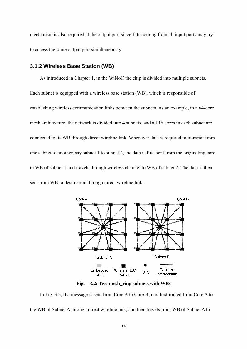
3.1.2 Wireless Base Station (WB)
As introduced in Chapter 1, in the WiNoC the chip is divided into multiple subnets.
Each subnet is equipped with a wireless base station (WB), which is responsible of
establishing wireless communication links between the subnets. As an example, in a 64-core
mesh architecture, the network is divided into 4 subnets, and all 16 cores in each subnet are
connected to its WB through direct wireline link. Whenever data is required to transmit from
one subnet to another, say subnet 1 to subnet 2, the data is first sent from the originating core
to WB of subnet 1 and travels through wireless channel to WB of subnet 2. The data is then
sent from WB to destination through direct wireline link.
Fig. 3.2: Two mesh_ring subnets with WBs
In Fig. 3.2, if a message is sent from Core A to Core B, it is first routed from Core A to
the WB of Subnet A through direct wireline link, and then travels from WB of Subnet A to
14
WB of Subnet B through wireless channel; finally, the message is sent to Core B from WB of
Subnet B through direct wireline link.
3.1.3 Network construction (Software perspective)
In this section, we will view the network construction and routing from a software
perspective. The following code is taken from our simulator as an example of how the
network construction and routing is done in the software level.
Network Construction (Mesh architecture with WB)
for (int a=0;a<numIps;a++){ // injection links
ports[current_switch_port_index].next = next_switch_port_index;
ports[next_switch_port_index].next = current_switch_port_index;
}
// =========== Connect all cores to WB =================
for (int i=0; i<(numIps-1); i++){
ports[current_switch_port_index].next = WB_port_index;
ports[WB_port_index].next = current_switch_port_index;
}
// ================================================
// ===============================================
The above code creates bi-directional connections between all cores in a subnet and their
associate switch, and also between all cores and WB. The statement ports[X].next = Y
specifies the current switch port X is connected to switch port Y. X and Y are port indexes
within a subnet. For a traditional mesh without WB, the Connect all cores to WB section of
the code has to be omitted.
15

3.2 Traffic Injection
The traffic is first generated by each embedded core and then injected it into its
associated switches. The frequency of generating a flit is determined by the traffic load of the
NoC. If the traffic load is high, the flits will be injected into the system more frequently. The
destinations of the generated flits are determined by the traffic pattern described below.
3.2.1 Uniform Random Traffic:
Traffic is uniformly and randomly distributed among the constituent embedded cores.
Every embedded core can be source or destination with equal probabilities.
3.2.2 Localization
The traffic localization restricts possible destinations of a given source. For
example, with localization factor 0.1, the destination of 10% of the traffic will be
restricted to only the given source’s neighboring cores and the destination of the other
90% of the traffic will be randomly distributed among other cores excluding its
neighboring cores.
Below gives an example of software level implementation of localization in mesh
architecture.
16

r = float_rand(1);
// =============== Part A ===============
if (r < localization_factor) {
while (loop){
loop = false;
for (int c=0; c < dimensions; c++)
msgs[i].dest[c]=int_rand(cube_dimensions[c]);
if (get_cube_address(msgs[i].dest)==get_cube_address(msgs[i].source))
loop=true;
if (get_cube_dist_mesh(msgs[i].dest,msgs[i].source)!=1)
loop=true;
}
}
// ====================================
// =============== Part B ===============
else {
while (loop){
loop = false;
for (int c=0; c < dimensions; c++)
msgs[i].dest[c]=int_rand(cube_dimensions[c]);
if (get_cube_address(msgs[i].dest)==get_cube_address(msgs[i].source))
loop=true;
if (get_cube_dist_mesh(msgs[i].dest,msgs[i].source)==1)
loop=true;
}
}
// ====================================
bool loop=true;
17

The above code is used to generate destinations of the messages injected by each
code. When r < localization_factor (Part A), the messages’ destinations are localized
around the originating core. Otherwise, when r >= localization_factor (Part B), the
messages’ destinations will be randomly distributed among the rest of the cores. In
Part A, the loop keeps running until the following conditions
get_cube_address(msgs[i].dest)==get_cube_address(msgs[i].source) and
get_cube_dist_mesh(msgs[i].dest,msgs[i].source)!=1 are not satisfied. In the first
condition, get_cube_address(msgs[i].dest) tells us the destination core of a message
and get_cube_address(msgs[i].source) tells us the source core of a message. The first
condition is used to prevent the source and the destination of a message end up in the
same core. The second condition makes sure that the distance between the source core
and the destination core of a message is within one Manhattan distance, which means
the traffic is localized. Similar code is used in Part B, except the second condition is
now used for the purpose to prevent traffic being localized around the source core.
3.2.3 Injection Load
The load factor determines the portion of the traffic, in terms of the maximum
capacity, that is injected into the system. For example, load factor of 1 represents the
maximum capacity. Load factor of 0.1 means we will only be injecting 0.1 of the
maximum traffic into the system.
18

3.2.4 Injection Type
Self-Similar Traffic
In the simulator, the self-similar traffic can be generated by aggregating a large number
of ON-OFF message sources. The amount of time each message spends in the ON or the OFF
state is determined by the Pareto distribution, which shows long-range dependence property.
The Pareto distribution is defined as ,α−−= xxF 1)( 21 <<α . A message stays in the ON state
for ONxtONα
1
)1(−
−= and stays in the OFF state for OFFxtOFFα
1
)1(−
−= , where x is an uniformly
distributed random number between 0 and 1, 9.1=ONα , and 25.1=OFFα [2].
Poisson Traffic
The Poisson traffic injection period follows the following exponential PDF
⎩⎨⎧
=−
0)(
x
Xe
xfλλ
otherwisex 0≥
where λ is the traffic injection rate.
3.3 Traffic Routing & Consumption
There are two parts involved in routing the traffic. The first part is to route the flits
within a switch. According to flits’ destination, the algorithm will determine which port the
flit should travel next. The second part is to route the flits among switches. Depending on the
destination, the algorithm will find the next port in another switch and route the flit there.
The header flits play an important role in the simulator. They are used to establish a path
between source and destination and let the data flits travel through that path. The header flits
are routed based on the routing algorithm associated with each architecture. When the header 19

flit arrives at a switch, it will first be stored in the virtual channels. Then, the simulator will
look through every virtual channel of every port within that switch to find the stored header
flit and retrieve the destination information. According to the destination information, the
next port within the switch will be assign to the header flit. When the header flits encounter
collisions, which means two or more headers at the same switch intend to go to the same
destination port within the switch, a select function will be called to deal with the problem.
The methods that we use to determine which header flit has the priority to route through a
switch in a collision situation are port orders, oldest first, and highest priority. Port orders
means the header flits will route through the switch base on the order of the ports it’s at.
Oldest first means the header flits which have been held at the switch for the longest time
have the priority to go through. Highest priority means the header flits will route through the
switch based on the priority information stored in them. Once the header flit establishes a
path, the data flits follow it to the destination. The cores are constantly monitoring arrival of
header flits. If a core detects a header flit, it knows the following (N-1) flits will be the data
flits (N = 64). Therefore, it initializes a data consumption countdown and counting from 0 to
(N-2) to finish the consumption of one message.
3.4 Conclusion
In this chapter we elaborated the characteristics of the simulator used to explore the
performance trade-offs for the WiNoCs. We explained how the simulator is used to model
different components of the WiNoC. Beginning by introducing the network construction and
20

the switch architecture followed by the characteristics of the injection traffic, finally, the
routing mechanism and flit consumption process are explained. In the next chapter, we will
use the simulator to evaluate the performance of WiNoCs and traditional NoCs.
21

Chapter 4
Performance evaluation
In this chapter, our aim is to evaluate performance of the WiNoCs compared to the
conventional 2D wireline and 3D mesh-based NoC architectures. Here we are principally
concerned with the network-level characteristics. Consequently the performance metrics
considered in this evaluation are the network throughput and latency. These two parameters
are defined below:
4.1 Performance Metrics
Latency: Latency is defined as the time period between the injection of a message’s
header flit and the reception of the same message’s tail flit at the destination core. In the
simulator described in chapter 3, the latency is obtained in units of clock cycles.
Throughput: Throughput is a metric that quantifies the rate at which message traffic can
be sent across a communication fabric. It is defined as the average number of flits arriving
per embedded core per clock cycle, so the maximum throughput of a system is directly
related to the peak data rate that a system can sustain. Accordingly, it is important to note
that a throughput of 1 corresponds to every node accepting one flit in every clock cycle.
22

4.2 Experimental setup
Simulator parameters Number of embedded cores 64 Buffer Depth (flits) 2 Virtual Channels 4 Message Length (flits) 64 Flit size 32 bits
Table 4.1: Simulator parameters
To carry out the evaluation process we considered a system with 64 embedded cores
and mapped them to different architectures under consideration. The experimental parameters
are shown in Table 4.1. Each switch port has 4 virtual channels and each of them can store up
to 2 flits. A single message consists of 64 flits and each flit is of size 32bits.
As mentioned in Chapter 1, for the wireless NoC, the whole network is divided into 4
subnets and each subnet consists of 16 cores. Intra-subnet communications are all based on
traditional wireline links while inter-subnet communications are done through wireless
channels. All the subnets have a wireless base station (WB), which is responsible for
establishing the wireless channels among the subnets. Two subnet architectures of WiNoC are
considered: mesh and hybrid ring-star.
Mesh
In this topology the cores in a subnet are interconnected among themselves by a
wireline mesh network. This mesh subnet has NoC switches and links as in a standard mesh
based NoC. Packet routing within the subnet follows dimension order (e-cube) routing. In
23

addition to this underlying mesh all the individual switches have direct wireline links to a
WB as shown in Fig. 4.1 (a).
Hybrid Ring-Star
In this subnet topology all the cores are connected on a ring to two nearest neighbors on
either side through conventional wireline NoC switches. In addition there is a central switch
which is attached to all the cores as well as the WB as shown in Fig. 4.1 (b). The central
switch provides additional connectivity compared to a simple ring structure. Data routing
follows a simple algorithm wherein, if the destination core is within two hops on the ring
from the source then the data is routed along the ring. If the destination core is more than two
hops away then the data routing takes place via the central switch. Thus within the subnet
each core is at a distance of at most two hops from any other core. The central switch is
connected to the WB and all inter-subnet packets are routed to the WB from the central
switch.
The performance of the two above mentioned WiNoCs are compared with traditional 2D
wireline mesh, wireline BFT, and wireline hierarchical mesh. In the hierarchical mesh, the
whole network is divided into 4 subnets. All the switches in each subnet connect to 4 of their
neighboring switches and connect to two additional switches in two other subnets as shown in
Fig. 4.1 (c). For clarity not all connections are shown in Fig. 4.1 (c). The extra connectivity of
each switch reduces the hop count between source and destination. This factor contributes to
the improved throughput and latency characteristic compare to a traditional wireline mesh. 24
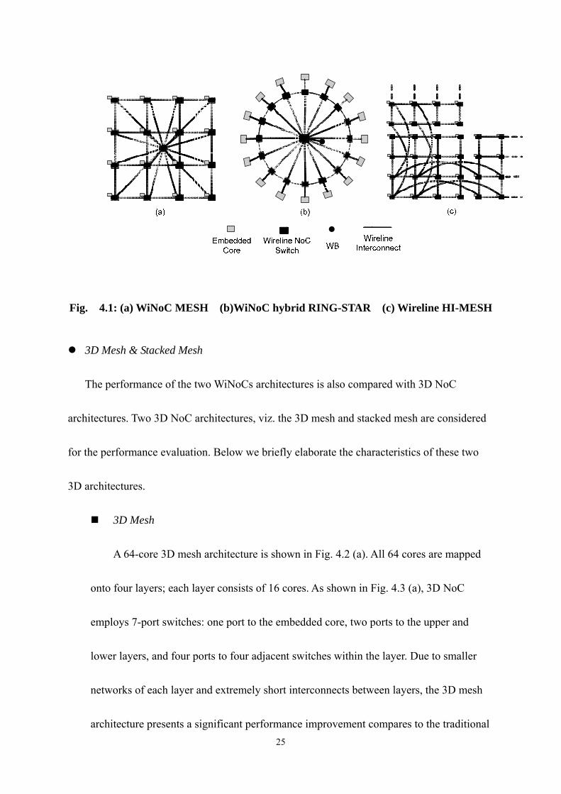
Fig. 4.1: (a) WiNoC MESH (b)WiNoC hybrid RING-STAR (c) Wireline HI-MESH
3D Mesh & Stacked Mesh
The performance of the two WiNoCs architectures is also compared with 3D NoC
architectures. Two 3D NoC architectures, viz. the 3D mesh and stacked mesh are considered
for the performance evaluation. Below we briefly elaborate the characteristics of these two
3D architectures.
3D Mesh
A 64-core 3D mesh architecture is shown in Fig. 4.2 (a). All 64 cores are mapped
onto four layers; each layer consists of 16 cores. As shown in Fig. 4.3 (a), 3D NoC
employs 7-port switches: one port to the embedded core, two ports to the upper and
lower layers, and four ports to four adjacent switches within the layer. Due to smaller
networks of each layer and extremely short interconnects between layers, the 3D mesh
architecture presents a significant performance improvement compares to the traditional 25
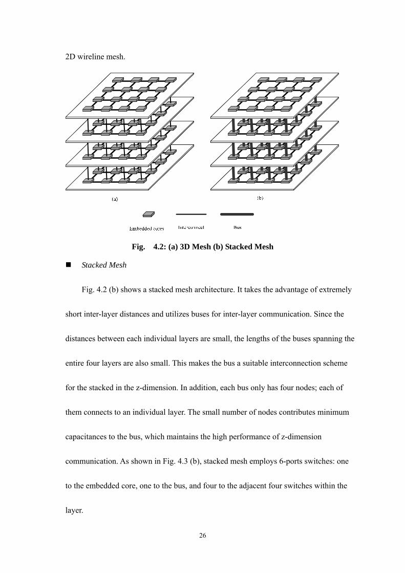
2D wireline mesh.
Fig. 4.2: (a) 3D Mesh (b) Stacked Mesh
Stacked Mesh
Fig. 4.2 (b) shows a stacked mesh architecture. It takes the advantage of extremely
short inter-layer distances and utilizes buses for inter-layer communication. Since the
distances between each individual layers are small, the lengths of the buses spanning the
entire four layers are also small. This makes the bus a suitable interconnection scheme
for the stacked in the z-dimension. In addition, each bus only has four nodes; each of
them connects to an individual layer. The small number of nodes contributes minimum
capacitances to the bus, which maintains the high performance of z-dimension
communication. As shown in Fig. 4.3 (b), stacked mesh employs 6-ports switches: one
to the embedded core, one to the bus, and four to the adjacent four switches within the
layer.
26

Fig. 4.3: Switche architectures of (a) 3D Mesh, (b) Stacked Mesh
4.3 Experimental Results: Throughput & Latency
To evaluate the performance of WiNoCs, traditional 2D wireline NoCs, and 3D
mesh-based NoCs, we consider the throughput and latency characteristics of 64 cores base
NoCs. Here, we evaluate two WiNoC architectures (hybrid ring-star, mesh), three completely
wireline architectures (mesh, BFT, and hierarchical mesh), and two 3D mesh-based
architectures (3D mesh, stacked mesh).
4.3.1 Throughput vs. Injection Load
The following two figures show the throughput characteristics of different NoC
architectures with respect to injection load. Injection load is defined by the number of flits
injected by each core per cycle. Fig. 4.4 shows the comparison between WiNoC architectures
and wireline 2D architectures.
27

00.10.20.30.40.50.60.70.80.9
0.1 0.2 0.3 0.4 0.5 0.6 0.7 0.8 0.9 1
Injection Load
Thro
ughp
uts
WiNoC_RING - STARWiNoC_MESHWireline_2D_MESHWireline_BFTWireline_HI - MESH
Fig. 4.4: Throughput vs. Injection Load (comparison with 2D NoCs)
0
0.1
0.2
0.3
0.4
0.5
0.6
0.7
0.8
0.9
0.1 0.2 0.3 0.4 0.5 0.6 0.7 0.8 0.9 1
Injection Load
Thro
ughp
ut
WiNoC_MESHWiNoC_RING - STAR3D MeshStacked Mesh
Fig. 4.5: Throughput vs. Injection Load (comparison with 3D NoCs)
Fig. 4.4 clearly shows the throughput advantage of WiNoC compare to traditional 2D
wireline architectures. This is due to the fact that wireless links between the subnets
affectively reduce the hop count while communicating between two long distance cores. In
other words, the flits in WiNoC need to travel less stage between a pair of source and
destination than traditional 2D wireline architectures. Since average hop count of wireline
BFT and wireline mesh is higher due to multi-hop communication, we see wireline BFT and 28

mesh performance worse in this category. On the other hand, hierarchical mesh is the only
completely 2D wireline architecture which has similar throughput characteristic as that of
WiNoC. It is due to the increased connectivity of hierarchical mesh, which effectively reduce
the hop count between two far away cores.
Fig. 4.5 depicts the comparative evaluation between the WiNoC architectures and 3D
mesh-based architectures. It shows the throughput advantage of WiNoC compared to the 3D
mesh-based architectures. However, the 3D architecture is able to closely match the
throughput performance of WiNoCs due to its high efficiency z-dimension communication,
which reduces the hop counts when communicating between two far away cores. As shown in
[21], the authors determined the average hop count of the 64-core 3D mesh to be 3.51, which
has a 40% reduction compare to 5.33 average hop count of the 64-core 2D wireline mesh. As
a result, we can expect a corresponding increase in throughput of the 3D mesh, which shows
in Fig. 4.5. Also notice that stacked mesh performs slightly better than 3D mesh. It is because
the z-dimension bus of the stacked mesh reduces the hop counts of inter-layer communication
slightly compare to those of 3D mesh. Between 2 WiNoC architectures, the hybrid ring-star
architecture performs better than the mesh architecture. It is due to the higher connectivity of
hybrid ring-star architecture, which means the average hop count of hybrid ring-star is lower.
Also notice that as we increase the injection load, wireline BFT and wireline MESH saturate
very quickly resulting in low throughput. On the other hand, 2 WiNoC architectures, wireline
hierarchical mesh, and 3D architectures can handle way more traffic. 29
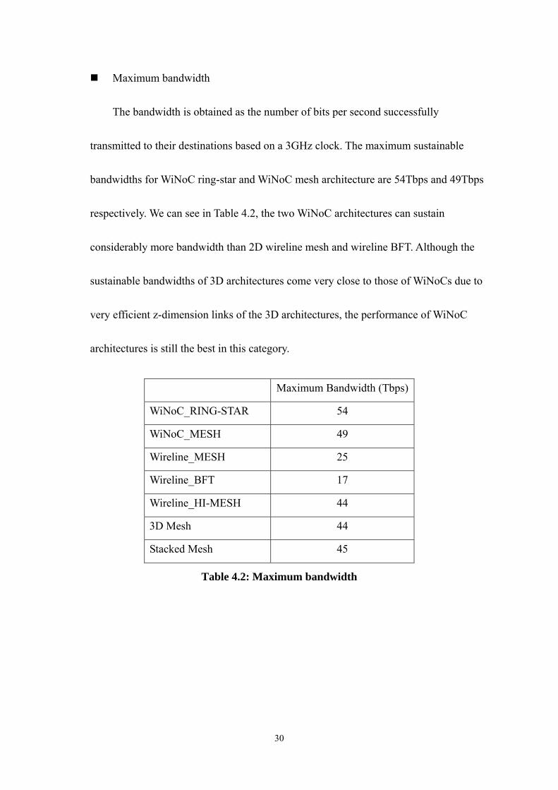
Maximum bandwidth
The bandwidth is obtained as the number of bits per second successfully
transmitted to their destinations based on a 3GHz clock. The maximum sustainable
bandwidths for WiNoC ring-star and WiNoC mesh architecture are 54Tbps and 49Tbps
respectively. We can see in Table 4.2, the two WiNoC architectures can sustain
considerably more bandwidth than 2D wireline mesh and wireline BFT. Although the
sustainable bandwidths of 3D architectures come very close to those of WiNoCs due to
very efficient z-dimension links of the 3D architectures, the performance of WiNoC
architectures is still the best in this category.
Maximum Bandwidth (Tbps)
WiNoC_RING-STAR 54
WiNoC_MESH 49
Wireline_MESH 25
Wireline_BFT 17
Wireline_HI-MESH 44
3D Mesh 44
Stacked Mesh 45
Table 4.2: Maximum bandwidth
30

4.3.2 Latency vs. Injection Load
0
200
400
600
800
1000
0.1 0.2 0.3 0.4 0.5 0.6 0.7 0.8 0.9 1
Injection Load
Late
ncy
WiNoC_RING - STARWiNoC_MESHWireline_2D_MESHWireline_BFTWireline_HI - MESH
Fig. 4.6: Latency vs. Injection Load (comparison with 2D NoCs)
0
200
400
600
800
1000
0.1 0.2 0.3 0.4 0.5 0.6 0.7 0.8 0.9 1
Injection Load
Late
ncy
WiNoC_MESHWiNoC_RING - STAR3D MeshStacked Mesh
Fig. 4.7: Latency vs. Injection Load (comparison with 3D NoCs)
The latency characteristic of the network is closely related to the throughput
characteristic. When the throughput of a network increases, the latency of it decreases. As
shown in Fig. 4.6 and Fig. 4.7, the 2 WiNoC architectures have the lowest latency among all
architectures. This shows the same performance advantages of WiNoCs as seen in the
previous section.
31

4.3.3 Throughput vs. Traffic Localization
For the previous analysis, we assumed that the traffic is random and uniformly
distributed among all the embedded cores. However, in a NoC, different functions are
mapped to different parts of the chip. Hence, the traffic is expected to be localized to different
degrees. We therefore study the effects of traffic localization on performance of WiNoCs,
traditional 2D wireline NoCs, and 3D mesh-based architectures.
In BFT, the localized traffic is constrained to within the cluster of each sub-tree. In
WiNoC mesh, 2D wireline mesh, and 3D mesh, the localized traffic is constrained to within
the destination located at the shortest Manhattan distance. In WiNoC ring-star, the destination
of the localized traffic is limited to two adjacent cores of its originated core.
In stacked mesh architecture, Li et al.[22] suggested much of the traffic should occur in
z-dimension to take advantage of high efficiency buses. As a result, processor and memories
are often place along the z-dimension because a large portion of the traffic occurs between
them. In this case, the traffic will be highly localized. Therefore, we consider the localized
traffic for stacked mesh to be constrained within the z-dimension buses.
The following two figures show the throughput characteristics of different NoC
architectures with respect to traffic localization. Fig. 4.8 compares the performance between
WiNoC architectures and wireline 2D architectures. Fig. 4.9 compares the performance
between WiNoC architectures and 3D mesh-based architectures.
32

0.2
0.3
0.4
0.5
0.6
0.7
0.8
0.9
0.1 0.2 0.3 0.4 0.5 0.6 0.7 0.8 0.9 1
Traffic Localization
Thr
ough
put
WiNoC_RING - STARWiNoC_MESHWireline_BFTWireline_MESHWireline_HI - MESH
Fig. 4.8: Throughput vs. Traffic Localization (comparison with 2D NoCs)
0.2
0.3
0.4
0.5
0.6
0.7
0.8
0.9
0.1 0.2 0.3 0.4 0.5 0.6 0.7 0.8 0.9 1
Traffic Localization
Thr
ough
put
WiNoC_RING - STARWiNoC_MESH3D MeshStacked Mesh
Fig. 4.9: Throughput vs. Traffic Localization (comparison with 3D NoCs)
Fig. 4.8 depicts the effects of traffic localization on throughput. The 2 WiNoCs still
possess performance advantage among the best in this category. As seen in Fig. 4.8, the
throughputs of wireline BFT and wireline mesh improve significantly while localized traffic
is applied. For wireline BFT, because of the highly localized traffic within each sub-tree, the
average hop counts between source and destination reduce considerably. The average hop
counts of wireline mesh also reduces as the traffic localization increases resulting in 33

performance boost. However, in order to achieve comparable bandwidth with the WiNoCs
and 3D NoCs, we have to have at least 70% of localized traffic.
Notice that the throughput characteristic of the two WiNoC architectures does not
improve much by traffic localization. Their throughput only increase slightly with higher
localization factor. This is because of the average hop counts of the WiNoC architectures are
already low, they can not reduce much more due to localized traffic. With traffic localization,
the maximum sustainable bandwidth of WiNoC hybrid ring-star becomes 55Tbps which only
has 1.8% gain compares to 54Tbps maximum bandwidth of the non-localized hybrid ring-star.
For WiNoC mesh, the maximum bandwidth becomes 53Tbps which has 8.2% gain compares
to 49Tbps maximum bandwidth of the non-localized mesh. We can see that WiNoC mesh
benefits more from localized traffic.
With traffic localization, the bandwidths of 3D mesh and stacked mesh increase to
52Tbps and 51Tbps respectively. As seen in Fig. 4.9, 3D architectures have very similar
throughput characteristics as those of WiNoCs. The performance of the 3D architectures also
does not improve much with localized traffic. It is because the already low averages hop
counts that do not scale very well with localized traffic.
34

4.3.4 Latency vs. Traffic Localization
0
500
1000
1500
2000
2500
3000
3500
4000
4500
0.1 0.2 0.3 0.4 0.5 0.6 0.7 0.8 0.9 1
Traffic Localization
Lat
ency
WiNoC_RING - STARWiNoC_MESHWireline_BFTWireline_MESH
Fig. 4.10: Latency vs. Traffic Localization (comparison with 2D NoCs)
0
500
1000
1500
2000
0.1 0.2 0.3 0.4 0.5 0.6 0.7 0.8 0.9 1
Traffic Localization
Lat
ency
WiNoC_RING - STARWiNoC_MESH3D MeshStacked Mesh
Fig. 4.11: Latency vs. Traffic Localization (comparison with 3D NoCs)
Fig. 4.10, demonstrates that the 2 WiNoC architectures have great latency characteristics.
We see that, in Fig. 4.10 and Fig. 4.11, the latency performances of all the architectures are
very similar except for wireline BFT and wireline mesh. This agrees with the observations we
got in the previous section.
35

4.4 Conclusion
In this chapter, we have evaluated throughput and latency characteristics of two WiNoC
architectures (hybrid ring-star, mesh) with respect to three conventional 2D wireline
architectures (mesh, BFT, HI-mesh) and 3D mesh-based architectures (3D mesh, stacked
mesh). The simulation results show the WiNoC architectures have much better performance
than traditional 2D wireline mesh and wireline BFT. This is due to the fact that wireless links
between the subnets affectively reduce the hop count while communicating between two long
distance cores. The performance of the wireline HI-mesh architecture is close to those of
WiNoCs due to the increased connectivity of hierarchical mesh, which reduces the hop count
between two far away cores. Also, 3D architectures present similar performance as that of
WiNoCs. It is because when communicating between 2 long distance cores, the high
efficiency z-dimension links affectively reduce the hop counts between the 2 cores, and
therefore improves the performance of the 3D architecture
36

Chapter 5
Conclusions and Future work
5.1 Conclusions
The current trend in System-on-Chip (SoC) design is to integrate numerous numbers of
embedded cores in a single die. The biggest challenge in the design of such massive
multicore chips is their interconnection infrastructure. The Network-on-Chip (NoC) paradigm
has emerged as an enabling methodology to design the interconnect architecture for
multi-core chips. In spite of all its advantages, traditional wire-based NoC employs multi-hop
communication, wherein the data transfer between two long distance cores gives rise to high
latency and energy dissipation. These problems can be resolved if the long distance multi-hop
communication links in a NoC are replaced with single-hop high-bandwidth wireless links.
In this thesis, we have demonstrated the performance advantages of two WiNoC
architectures (hybrid ring-star, mesh) in terms of network-centric parameters, like throughput
and latency by comparing them with traditional 2D wireline NoCs (BFT, mesh, Hi-mesh) and
3D mesh-based architectures (3D mesh, stacked mesh). We developed a versatile simulator,
which can be used to obtain the performance of the wireless NoCs (WiNoCs) under various
realistic traffic conditions. This simulator can accept various network architectures and traffic
patterns (both spatial and temporal) as inputs and it predicts the performance of the WiNoCs.
This kind of simulator helps the designer to quickly obtain a rough estimate of the expected
37

performance and the resources used for any WiNoC architectures. With the help of this
simulator we have evaluated all the above architectures in terms of their throughput and
latency characteristics while varying traffic injection load and traffic localization factor. In
chapter 4 we have shown that, without any kind of traffic localization, the maximum
bandwidth of WiNoC ring-star and WiNoC mesh are 54 Tbps and 49 Tbps respectively. This
performance is much higher than the traditional 2D wireline mesh and BFT architectures,
which is only 25 Tbps and 17 Tbps respectively. In order for the 2D wireline mesh and BFT
architectures to match the performance of WiNoCs, at least 70% localized traffic has to be
employed. 3D mesh-based architectures, on the other hand, have much better performances
than the conventional 2D mesh and BFT. 3D mesh and stacked mesh architectures achieve
maximum bandwidths of 44 Tbps and 45 Tbps respectively. With localized traffic, the 3D
mesh-based architectures can almost match the performances of WiNoCs.
5.2 Future Work
The research performed for this thesis has several far reaching directions as discussed below:
5.2.1 Optimization of network configuration
In this thesis, the network of WiNoC is divided into four equal quadrants; each one is
defined as a subnet. Under a given network size, there are various ways of arranging the
subnets as well as the subnet size. The optimal way of setting up the subnets is yet to be
studied.
38

5.2.2 Comparison among all alternatives
In addition to WiNoCs and 3D architectures, investigations regarding photonic NoCs [5,
12] and RF-interconnect NoCs [6, 11] have been done as potential alternatives to traditional
2D wireline architectures. Although the research of photonic NoC shows a promising
sustainable bandwidth, problems such as fabrication difficulty of the on chip wave guides and
optical switch mechanism still need further investigation. Also, it is a challenge for
RF-interconnect based NoCs to place multiple very high frequency oscillators and filters on
chip. Given that each alternative has its own advantages and shortcomings, a comprehensive
comparison among all these alternatives needs to be performed.
For a comprehensive comparison, throughput and latency are not the only concerns.
Though latency and throughput characterize a network, but for an on-chip network the
following parameters are important factors and they need to be considered for a complete and
exhaustive performance evaluation.
Power Dissipation
In traditional wireline NoCs, the interconnect infrastructure dissipates a large percentage of
power. This is shown to approach 50% in some applications [23]. Therefore, the power
dissipation is a key factor for all the emerging alternative NoC architectures. Though the 3D,
Photonic and RF-interconnect based NoCs are shown to be more power efficient than
traditional planar NoCs, but how they will perform compared to a WiNoC is a very important
concern. Success of WiNoC paradigm will depend on how it performs with respect to this
39

parameter.
Fabrication Difficulty
The success of all these emerging technologies will depend on their manufacturability. So far
both 3D and Photonic NoCs suffer from manufacturability issues. One serious factor
influencing the transition towards 3-D integrations is die yield, which in the case of 3-D
circuits depends on factors like pattern mismatch between different layers and vertical via
failure. An additional difficulty is to be able to fabricate the subsequent layers or add them to
the IC without damaging the already-existing layers. For instance, high-temperature
processes such as thermal growth and diffusion can severely affect the previous layers. Also,
one faulty layer can cause the whole 3D assembly to fail, reducing the overall yield.
Consequently increasing the number of active layers affects the yield of a 3D chip. Similarly
though there is tremendous progress in silicon photonics for the last few years, but still the
technology to integrate all the necessary components of a Photonic NoC in a single die is far
from mature. Comparatively the RF-interconnect based NoC can be designed using existing
CMOS technologies. In case of WiNoC if we depend on on-chip RF antennas then also there
are no big manufacturability issues. But if the advantages of emerging carbon nanotube
antennas need to be exploited to design the WiNoC then that will again involve different
manufacturing issues. All these factors need to be incorporated for a complete performance
evaluation
40

Area Overhead
The silicon area overhead for all these emerging NoCs need to be considered. Area overhead
arising from the NoC switches, integration of various components, like antennas, photonic
components etc. need further examination.
Heat Dissipation
Heat dissipation is a key factor that affects the stability of a chip. This is a potential problem
for 3D NoCs. Due to 3D structure, the size of each layer in 3D NoC is reduced. It results in a
sharp increase in power density. As mention previously, the interconnect infrastructure
dissipates a large percentage of power. Therefore, the major heat dissipation of 3D NoC
comes from the interconnection network. While evaluating performance of WiNoC with 3D
NoCs heat dissipation needs to be accounted for.
5.3 Summary
NoC has emerged as an enabling methodology for integration of huge number of
embedded cores on a single die. The interconnect infrastructure is known as the performance
bottleneck of traditional 2D wireline NoCs. In this thesis, we have proposed an alternative
architecture (WiNoC) to resolve this problem. We have demonstrated that the performance of
the WiNoCs has significant improvement compare to the traditional 2D wireline NoCs. We
also compared the performance of the WiNoCs to the 3D mesh-based NoCs, which is known
to have a significant performance gain over the traditional 2D wireline architecture. WiNoCs
still possess its performance advantages against 3D mesh-based architectures.
41

BIBLIOGRAPHY[1] L. Benini and G. De Micheli, "Networks on chips: A new SoC paradigm," Computer,
vol. 35, pp. 70-+, Jan 2002. [2] P. P. Pande, C. Grecu, M. Jones, A. Ivanov, and R. Saleh, "Performance evaluation
and design trade-offs for network-on-chip interconnect architectures," Ieee Transactions on Computers, vol. 54, pp. 1025-1040, Aug 2005.
[3] S. R. Vangal, J. Howard, G. Ruhl, S. Dighe, H. Wilson, J. Tschanz, D. Finan, A. Singh, T. Jacob, S. Jain, V. Erraguntla, C. Roberts, Y. Hoskote, N. Borkar, and S. Borkar, "An 80-tile sub-100-W TeraFLOPS processor in 65-nm CMOS," Ieee Journal of Solid-State Circuits, vol. 43, pp. 29-41, Jan 2008.
[4] V. F. Pavlidis and E. G. Friedman, "3-D topologies for networks-on-chip," Ieee Transactions on Very Large Scale Integration (Vlsi) Systems, vol. 15, pp. 1081-1090, Oct 2007.
[5] A. Shacham, K. Bergman, and L. P. Carloni, "Photonic networks-on-chip for future generations of chip multiprocessors," Ieee Transactions on Computers, vol. 57, pp. 1246-1260, Sep 2008.
[6] M. F. Chang et al, "CMP Network-on-Chip Overlaid With Multi-Band RF-Interconnect," Proceedings of IEEE International Symposium on High-Performance Computer Architecture (HPCA), pp. 191-202, 16-20 February 2008.
[7] K. Kempa, J. Rybczynski, Z. P. Huang, K. Gregorczyk, A. Vidan, B. Kimball, J. Carlson, G. Benham, Y. Wang, A. Herczynski, and Z. F. Ren, "Carbon nanotubes as optical antennae," Advanced Materials, vol. 19, pp. 421-+, Feb 5 2007.
[8] J. J. Lin, H. T. Wu, Y. Su, L. Gao, A. Sugavanam, J. E. Brewer, and K. O. Kenneth, "Communication using antennas fabricated in silicon integrated circuits," Ieee Journal of Solid-State Circuits, vol. 42, pp. 1678-1687, Aug 2007.
[9] P. P. Pande, C. Grecu, A. Ivanov, and R. Saleh, "Design of a Switch for Network on Chip Applications," Proc. Int'l Symp. Circuits and Systems (ISCAS) vol. 5, pp. 217-220, May 2003.
[10] A. W. Topol, D. C. La Tulipe, L. Shi, D. J. Frank, K. Bernstein, S. E. Steen, A. Kumar, G. U. Singco, A. M. Young, K. W. Guarini, and M. Ieong, "Three-dimensional integrated circuits," Ibm Journal of Research and Development, vol. 50, pp. 491-506, Jul-Sep 2006.
[11] M. F. Chang et al., "RF Interconnects for Communications On-Chip," Proceedings of International Symposium on Physical Design, pp. 78-83, 13-16 April 2008.
[12] M. J. Kobrinsky et al., "On-chip optical interconnects," Intel Tech. J., vol. 8, pp. 129-142, May 2004.
[13] W. M. J. Green, M. J. Rooks, L. Sekaric, and Y. A. Vlasov, "Ultra-compact, low RF
42

power, 10 gb/s silicon Mach-Zehnder modulator," Optics Express, vol. 15, pp. 17106-17113, Dec 10 2007.
[14] D. Zhao and Y. Wang, "SD-MAC: Design and synthesis of a hardware-efficient collision-free QoS-aware MAC protocol for wireless Network-on-Chip," Ieee Transactions on Computers, vol. 57, pp. 1230-1245, Sep 2008.
[15] G. W. Hanson, "On the applicability of the surface impedance integral equation for optical and near infrared copper dipole antennas," Ieee Transactions on Antennas and Propagation, vol. 54, pp. 3677-3685, Dec 2006.
[16] G. Y. Slepyan, M. V. Shuba, S. A. Maksimenko, and A. Lakhtakia, "Theory of optical scattering by achiral carbon nanotubes and their potential as optical nanoantennas," Physical Review B, vol. 73, pp. -, May 2006.
[17] P. J. Burke, S. D. Li, and Z. Yu, "Quantitative theory of nanowire and nanotube antenna performance," Ieee Transactions on Nanotechnology, vol. 5, pp. 314-334, Jul 2006.
[18] G. W. Hanson, "Fundamental transmitting properties of carbon nanotube antennas," Ieee Transactions on Antennas and Propagation, vol. 53, pp. 3426-3435, Nov 2005.
[19] Y. Huang, W. Y. Yin, and Q. H. Liu, "Performance prediction of carbon nanotube bundle dipole antennas," Ieee Transactions on Nanotechnology, vol. 7, pp. 331-337, May 2008.
[20] R. I. Greenberg and H. C. Oh, "Universal wormhole routing," Ieee Transactions on Parallel and Distributed Systems, vol. 8, pp. 254-262, Mar 1997.
[21] B. S. Feero and P. P. Pande, "Networks-on-Chip in a Three-Dimensional Environment: A Performance Evaluation," IEEE TRANSACTIONS ON COMPUTERS, vol. 58, pp. 32-45, January 2009.
[22] F. Li et al., "Design and Management of 3D Chip Multiprocessors Using Network-in-Memory," Proceedings of the 33rd International Symposium on Computer Architecture (ISCA), pp. 130-141, 2006.
[23] T. Theocharides et al., "Implementing LDPC Decoding on Network-On-Chip," Proceedings of the International Conference on VLSI Design, pp. 134-137, 2005.
43
Recommended