Market Structure and Dealer’s Quoting Behavior
In the Foreign Exchange Market
Liang Ding*
Department of Economics, University of North Carolina at Chapel Hill,
Chapel Hill, NC 27514, USA
Abstract
Noticing that the structure of customer and inter-dealer foreign exchange markets are
different, this paper examines the impact of the difference on the dealer’s quoting
behavior in both markets theoretically and empirically. We show that customer mid-quote
equals the inter-dealer one, and customer spread is wider than inter-dealer spread, while
their differential tends to fall with the rise in order size. In contrast to the preceding
models claiming that the order size has positive effect on the spread, the impact is found
to be ambiguous in our model. The testing of a new data set provides convincing
evidences in favor of theoretical conclusions.
JEL classification: F31; G14; G15
Keywords: foreign exchange market; market microstructure; bid-ask spread; order size.
* Corresponding author. Tel.: +1-919-914-6851; fax: +1-919-966-4986 Email address: [email protected] ( Liang (Leon) Ding ).
1
1. Introduction
The foreign exchange market (FX market) is a decentralized dealership market, where
market orders pass to an intermediary (dealer) for execution, and the price of currency is
created by quoting bid and ask prices in response to trading initiatives. Based on different
initiatives, the FX market can be divided into an inter-dealer (inter-bank) market in which
dealers (banks) trade with each other, and a customer market in which customers trade
with dealers. Accordingly, each dealer actually quotes two pairs of bid-ask prices in
practice: one for inter-dealer trading and the other for customers. The questions arising
are: does the dealer quote the same bid-ask prices in the two markets at any given point in
time? Furthermore, are his spreads and mid-quotes the same in the two markets? If not,
why are they different? How different are they? And, is there any empirical evidence to
show the difference?
These questions are important in both academic and practical senses. Since customer
and inter-dealer FX markets are characterized by different structures, the dealer’s quoting
decision in both markets is a perfect case to examine the impact of market microstructure
on the market participant’s behavior. Moreover, since it is about the same dealer’s
simultaneous quotes in the two markets, results will not be jeopardized by the change of
agent’s preference over time or the heterogeneity of various dealers. Practically, knowing
dealers’ quoting mechanisms is helpful for central banks to improve efficiency of
intervention and regulation. And also, it will help dealers make a reliable prediction and
evaluation on the effect of introducing new trading platforms or services to the FX
market.
To the questions noted above, unfortunately, the current literature has not yet
provided satisfying answers. On the theoretical level, many models have been devoted to
the problem of bid-ask quotes determination, but most of them are built originally for the
2
traditional stock markets1, which operate differently than the FX market. NYSE, for
instance, is a centralized auction market, where buyers enter competitive bids and sellers
enter competitive offers at the same time, and the price of stock is determined by an order
execution algorithm automatically matching buy and sell orders on a price and time
priority basis. Unlike the FX market, the stock markets do not have separate venues for
inter-dealer and customer trading, so it is understandable that these models do not make
such a differentiation, e.g. Ho and Stoll (1981), Biais (1993), Laux (1995), etc. On the
other hand, there do exist some models built specifically for the FX market in the
literature. However, these models either concentrate on the inter-dealer market alone, e.g.
Black (1991) and Bessembinder (1994), or just ignore the distinctions between the two
markets and assume dealers quote only one pair of bid-ask prices, e.g. Bollerslev and
Melvin (1994).
On the empirical level, a lot of data sets have been used to examine the bid-ask
prices determinants in the FX market. Glassman (1987) uses daily quotes of a single
Chicago futures dealer. Black (1991) exploits fixed rates in some European markets as
surveyed by the several central banks. Bollerslev and Domowitz (1993), Demos and
Goodhart (1996), Huang and Masulis (1999) as well as Hartmann (1999) have access to
continuous Reuters quotes. Bessembinder (1994) and Jorion (1996) use daily data from
the DRI data bank, which are Reuters quotes of a “representative” dealing bank at some
time during the day. Disregard to the variation in the sources, all of these data are only
the quotes for the inter-dealer trading. There is no prior use of a data set containing
customer quotes, not to mention comparing the inter-dealer quotes to the customer ones.
1 The stock markets in this paper are referring to NYSE and AMEX, which are centralized auction markets. Another security market NASDAQ, on the contrary, is more like a decentralized dealership market.
3
In order to answer the questions we are considering, effort is made theoretically and
empirically in this article. Following Biais (1993), I build a model viewing the dealer as a
risk aversion agent who chooses bid-ask prices to optimize his portfolio based on the
information he receives. In contrast to the preceding work focusing on the stock market,
the setup and assumptions of the model are made compatible with the environment and
structure of FX market. Moreover, the distinctions between the customer market and the
inter-dealer market will be identified and incorporated into the model. The dealer’s
quoting problems are solved in both markets, and the solutions of optimal bid-ask quotes
lead to the explicit form of spreads and mid-quotes, so that comparison can be made.
Empirically, a new data set has been collected, which contains both customer and inter-
dealer bid-ask quotes covering the same period and picked at the same frequency.
Applying the new data set, I test several theoretical conclusions implied by our model
and obtain convincing results.
Two major distinctions between the inter-dealer and customer FX markets are
theoretically identified in this paper. The first one is embodied in the difference of market
transparency. Compared to the inter-dealer market, where most transactions are
conducted through the electronic dealing system (e.g. Reuters) on which dealers
recognize the best quotes efficiently and almost costless, the customer market is
relatively more opaque, and it costs regular customers much more to find the best price
available and trade at it. This difference allows a margin for the dealer to keep the
customer spread generally wider than the inter-dealer one. The second is embodied in the
difference of information asymmetry. Since dealers are usually believed to be better
informed than customers, if the order size is larger, the dealer is more inclined to raise the
spread to deter adverse selection when trading with dealers than customers. Therefore,
the differential between the customer and the inter-dealer spreads decreases with the rise
in order size. In spite of these distinctions, as the dealer’s belief of the true value of
4
currency, his mid-quotes of bid-ask prices in the two markets are proved to be identical in
the model.
Empirically, our data verify the theoretical conclusions that customer spread is
generally wider than the inter-dealer spread, but the differential decreases with the rise in
order size. Furthermore, strong evidence has been found that mid-quotes of bid-ask prices
in the two markets are equal to each other. Meanwhile, disagreeing with most other
models indicating that spreads should be positively related to the order size, our results
show that the impact is ambiguous, for which our model provides reasonable
explanations too.
This article makes contributions to the literature in two major aspects. Theoretically,
noticing that the structure of the customer and inter-dealer foreign exchange markets are
different, the paper identifies those differences and incorporates them into a formal model.
As the solutions to the dealer’s quoting problem, the optimal bid-ask quotes in both
markets show clearly how different they are as well as why. Empirically, by employing a
data set characterized of several new features, I have tested some hypotheses that have
never been examined by real data before. To my knowledge, the paper makes the
empirical comparison between the inter-dealer and customer quotes for the first time in
the literature. And also, our research finds evidence that contradicts the existing claim
that people used to believe with regard to the relationship between the spread and the
order size.
The rest of the paper is structured as follows: section 2 presents a model describing
dealer’s quoting problem in the inter-dealer and customer FX markets respectively, and
shows the explicit form of the optimal bid-ask prices. Section 3 introduces the new data
set we collected and illustrates the empirical evidence of the model. Finally, section 4
concludes.
5
2. Theoretical framework of model
2.1 Setup and assumption
Our model describes a decentralized dealership market, in which dealers and
customers are the only market participants1. The FX market is divided into two sections:
dealers trade with each other in the inter-dealer market, and customers trade only with
dealers in the customer market.
We assume N dealers are active in the market, and each dealer’s preference is
represented by the regular utility function as below:
)exp()( WAWU ⋅−−=
where A is degree of risk aversion and W represents wealth
To stay in the business, dealer i pays the fixed cost iC , which accounts for the
operation expenses independent of number of transactions, e.g. the fee of connection to
the inter-dealer dealing system. Meanwhile, the rising scale of business increases
operation cost too. For instance, more staff needs to be hired to handle the increasing
number of transaction requests. Suppose the dealer assumes extra cost ω for handling one
more market order, and this cost is assumed to be fixed relative to the size of the order.
As the provider of liquidity, the dealer must hold inventory to facilitate transaction.
However, excessive position leads to higher risk, so the dealer always tries to keep the
position to some particular level, which guarantees normal transaction and minimizes risk.
This particular level is called as the ideal level of inventory, and we just assume it is
constant across periods and normalize it to zero for simplicity.
Our dynamic model focuses on one price adjustment period, in which real interest
rate is normalized to 1. The details about the timing of the model are as follows:
1) Initial status at the beginning of the period
1 Since electronic brokering system has replaced “voice brokers”, we just ignore the role of brokers.
6
At the beginning of the period, the dealer is endowed with cash and holds
inventory level . For each particular dealer, he definitely knows his own inventory level,
whereas inventory levels across the dealers are publicly unobservable and considered as
random variables, which are characterized by distribution function . For simplicity,
different dealers’ are assumed to be independently and identically distributed with
uniform distribution within [-R, R]
iK
iI
iF
iI1.
Since the FX market is continuously trading, before any new information is released,
the dealer’s status at the beginning of the current period is actually the same as that at the
end of the previous period. Hence, dealer i’s current quotes should be ones he made in the
previous period2. If the middle point of his bid-ask quotes in the last period is denoted
as , then, before any information observed at the beginning of the current period t, his
mid-quote should still be too.
1−tp
1−tp
2) Public information releasing
We assume the public information is released right after the beginning of the period
and observed by every agent in the market3. Public information refers to the information
available for all market participants, such as central bank announcements. Public
information systematically changes the customers and dealers’ expectations of exchange
rates, and the dealer will adjust his quote immediately to incorporate the information. If
the change in the exchange rate implied by the public information is denoted as , then
the dealer‘s quote becomes . Let denote the dealer’s mid-quote after releasing
tr
tt rp +−10p
1 Instead of the uniform distribution, it might be more appropriate to assume the inventory follows the normal distribution. However, the explicit form of normal distribution function is very hard to induce, if it is possible. To obtain relatively simple explicit form of solutions, I made this assumption. In fact, the fundamental relationships implied by the model will not be changed by just assuming another distribution. 2 In the security market, the opening price of a new day and the closing price at the previous day are often different. But in the FX market, it is reasonable to make such an assumption, as the market is continuously trading. 3 Another way to understand this assumption is separating the periods based on the release of public information.
7
the public information, then . Since the mid-quote of dealer’s bid-ask prices
is usually taken as the observation of exchange rate, becomes the current market
exchange rate and is observed by every agent in the market.
tt rpp += −10
0p
3) Market order arrives
Now, market order comes. Some agent contacts the dealer with potential order size
of Q and asks for quotes. The transaction initiative could be another dealer in the inter-
dealer market or one customer in the customer market. Suppose the initiator reveals a
tendency of buying or selling when asking for quotes, so that the dealer knows the order
size Q and direction of potential transaction before quoting1. This information is only
observed by the dealer himself and therefore becomes his private information.
No matter dealers or customers initiate the transaction, we assume their trading
requests are based on the difference between their own belief of the terminal exchange
rate in this period and the current prevailing exchange rate ( ). Furthermore, the sign of
such difference determines the direction of transaction (buy or sell), and order size is
proportional to the magnitude of the difference.
0p
4) Make the quote decision
As the response to the buying and selling request, the dealer needs to quote ask price
and bid price respectivelyiap +0ibp −0 2. Knowing the information of order size Q
and order direction, the dealer’s objective is to choose a and b to maximize his expected
utility in the inter-dealer and customer markets. The solutions to the problem will be his
optimal quotes in both markets.
1 Sometimes, dealers quote both bid-ask prices without knowing tendency of the transaction. But the dealer from whom I collected the data knows the tendency before displaying his quote. To be consistent with the data source, I make such an assumption. 2 Such a structure of the quotes makes the quoting problem symmetric and will facilitate our analysis later.
8
At this stage, we assume every dealer has to make quotes once being asked. In fact,
it is possible that in some circumstances dealers refuse to quote, probably because they
think the order is too large or the market is too volatile so that it is too risky to make
quotations. However, due to the fierce competition among the dealers in the FX market
today, very few would do so, as that will damage their reputation and scare customers
away. In the model, I ignore the issue of whether to quote or not, and assume dealers
always make quotes once being asked.
2.2 Dealer’s quoting problem and the optimal quotes in the inter-dealer market
Following Biais (1993), the dealer’s process of selecting optimal bid-ask quotes are
laid out by two steps. First, the bottom line for the dealer to make a quotation is that at
least he will not be worse off after revealing his quotes regardless accepted or not. The
quotes making him indifferent between trading and not trading are reservation quotes,
which the dealer will take as a benchmark. Second, the dealer apparently has incentive to
raise the ask (selling) price above or reduce the bid (buying) price below the reservation
quotes to earn extra profit; however, such a behavior will decrease the probability that the
quotes are accepted obviously. Therefore, there must be a point, which maximizes his
expected utility and becomes his optimal choice.
Now, suppose another dealer sends the buying request with the order size Q, and
dealer i quotes the ask price , in which superscript d denotes inter-dealer market.
At this moment, before the dealer reveals his quotes, as assumed before, he holds cash
and inventory .
diap +0
iK iI
If his quote is declined, and no transaction takes place, then the dealer’s cash holding
and inventory remain the same, however, the dealer still pays the fixed operation cost iC .
Suppose random variable z~ is the difference between the current prevailing exchange
9
rate and the exchange rate at the end of the period, the terminal value of the exchange
rate will be
0p
zp ~0 + , and the dealer’s terminal wealth can be written as:
)~()0( 0 zpICKW ++−= iii (1)
If his quote is accepted, and the transaction imitative buys Q at the ask price ,
then the dealer’s inventory falls by Q, cash holding rises by , and he pays the
extra operation cost in addition to
diap +0
Qap di )( 0 +
ω iC . If z~ is still defined as before, the dealer’s
terminal wealth after the transaction becomes:
QapzpQICKaW diiiii
di )()~)(()( 00 +++−+−−= ω (2)
Clearly the dealer’s expected wealth depends on the expected value of z~ , and the
dealer will certainly form the expectation about z~ conditioned on the information he
receives. According to our analysis before, the transaction initiative tending to buy Q
units of the currency implies that in his opinion the market exchange rate in the future
must be higher than the current one, i.e. )~(zE >0. Also, the order size Q should be
proportional to the )~(zE . Through a linear signal extraction process, the dealer factors
information set Sa into his own expectation of z~ as follows:
Sa= {some agent wants to buy Q units of the currency} and QSzE a ⋅= β)|~(
In the pervious equation, positive parameter β is used to measure how accurate the
transaction initiative’s expectation is in the dealer’s opinion. Given the same order size,
β is larger if the dealer believes that the agent asking for quotes is better informed1. In an
extreme case, if the dealer thinks the agent as a totally noise trader, and his transaction
request cannot reflect the true value of the exchange rate in the future at all, then theβ
would be zero. In this sense, the value of β actually reflects the dealer’s evaluation
about how well informed the transaction initiative is.
1 In the model of linear signal extraction,β is actually negatively related to the variance of expectation. If the agent is believed to be better informed, then his expectation variance will be smaller, soβ is larger.
10
According to its definition, the reservation quote should make quoting results
(trading or no trading) indifferent, i.e. the dealer’s conditional expected utility of the two
cases equal to each other. Suppose dealer i’s reservation ask price in the inter-dealer
market is denoted as , the following equation (3) should hold: dr
iap ,0 +
)|))((()|))0((( , adra SaWUESWUE = i (3)
Similarly, if another dealer sends selling request with the order size Q, the dealer
quotes bid price . If his quote is declined, the terminal wealth is the same as
shown in equation (1). If his quotes are accepted, the dealer’s terminal wealth will be:
dibp −0
QbpzpQICKbW diiii
di )()~)(()( 00 −−+++−−= ω (4)
In the selling case, the dealer will receive information set Sb and make expectation
about z~ as below:
Sb= {some agent wants to sell Q units of the currency} and QSzE b ⋅−= β)|~(
The reservation bid price will make equation (5) hold: dribp ,0 −
)|))((()|))0((( , bdrb SbWUESWUE = i (5)
The dealer’s reservations quotes, which are the solutions to equations (3) and (5),
are shown in the following lemma 1. The derivation process is attached in appendix I.
Lemma 1: Under our set of assumptions, dealer i’s reservation selling (ask) and
buying (bid) prices in the inter-dealer market are and , where )( ,0 driap + )( ,0 dr
ibp −
iddr
i IAQ
QAa ⋅−+⋅+= 22
, )2
( σωβσ
iddr
i IAQ
QAb ⋅++⋅+= 22
, )2
( σωβσ
Next, we derive the dealer’s optimal deviation from the reservation quotes. For each
buying request, the dealer revealing quotes leads to two possible results: accepted or not
accepted. In the first case, the dealer’s utility will be , while the utility
is in the second, where both wealth of portfolio is defined as before. The
)|))((( adi SaWUE
)|))0((( aSWUE
11
reason that we use expected utility even for each specific state is because the change in
the exchange rate, z~ , is still a random variable and will not be realized until the end of the
period. Let denote the probability that dealer i’s quote is accepted, then as usual, the
total expected utility for dealer i can be written as:
dia,π
(6) )|))0((()1()|))((( adia
adi
diaia SWUESaWUEEU ππ −+= ,,,
,
Currently, the major fraction of turnover in the inter-dealer market is conducted
through the electronic inter-dealer dealing system, such as Reuters D2000-2. The system
displays the real time information of the best bid-ask prices available on its screen, and
every dealer can observe it easily and almost costless. If dealer i is chosen to be bought
from, it usually means his ask price is lower than any other competitor’s. Accordingly,
the probability of other dealers accepting his quote is equivalent to the probability that his
ask price is the lowest among all the dealers, which can be expressed as
where subscript –i represents all other dealers. )(,di
di
dia aaP −<=π
Now, if the dealer’s current inventory is higher than the preferred level, i.e. I>0, it
suggests that the dealer holds more position than he would like to. In order to reduce the
inventory, quoting lower price is an efficient strategy to encourage selling and deter
buying. On the contrary, if the current inventory is lower than preferred level, i.e. I<0,
the dealer intends to increase the price in order to sell less or buy more, so that the
inventory will move up to the ideal level. Therefore, we claim that to all dealers the
optimal quoting strategy should be decreasing to each dealer’s inventory level I.
Since the dealer’s optimal quoting strategy is decreasing to the inventory, the
probability that the dealer’s ask price is lower than others is equivalent to the probability
that his inventory is larger than others, i.e. . Using the
assumption that the dealers’ inventory levels are random variables with the identical and
independent uniform distributions F
)()( iidi
di
dia IIPaaP −− >=<=π
i within [-R, R], the probability can be expressed as:
12
1, )
2()()()( −
≠−−
+==>=<= ∏ Ni
N
ijijii
di
di
dia R
RIIFIIPaaPπ (7)
Now, go back to the original quoting problem. Rearranging equation (6) gives
equation (8): (8) )|))0((()]|))0((()|))((([,aaad
id
ia SWUESWUESaWUEEU +−= π
According to the definition of the reservation quote, equation (9) must hold:
(9) QaaAaadi
dri
dieSWUESaWUE )( ,
)|))0((()|))((( −−=
Substituting equation (9) to equation (8) gives:
(10) )|))0((()|))0((()1( )(,
, aaQaaAdia SWUESWUEeEU
dri
di +−= −−π
Since does not depend on the choice of the ask price, it can be
neglected from the objective function, and the aim of the dealer will be simplified as:
)|))0((( aSWUE
(11) )1( )(,
,
−−− QaaAdia
a
dri
di
di
eMaxπ
Finally, the linear approximation of objective function (11) by Taylor expansion
gives: ))(( ,
, QaaAMax dri
di
dia
adi
−π (12)
Where is defined in equation (7) d
ia,π
Objective function (12) demonstrates the dilemma that the dealer is facing when he
chooses quotes. On one hand, higher ask price ( ) relative to the reservation quote
( ) is justified by a higher value of the objective function and potential profit. On the
other hand, it reduces the probability of the quote being accepted ( ) for obvious
reasons. Hence, there must be an optimal ask price that maximizes the objective, which
will be the dealer’s choice.
dia
dria ,
dia ,π
The analysis above describes the process of selecting the ask price when the dealer
receives the buying request. Due to the symmetric setup of bid-ask quotes, the optimal
bid price can be determined similarly.
Following Biais (1993)’s general proof, I derive the explicit form of dealer i's
optimal bid-ask quote in the inter-dealer market and show them in proposition 1.
13
Proposition 1: Under our set of assumptions, the solutions to the dealer’s problem
and the optimal bid and ask prices of dealer i in the inter-dealer market are
and , where
)( 0 dibp −
)( 0 diap +
NIRAaa idr
idi
+⋅+= 2, σ
NIR
Abb idri
di
−⋅+= 2, σ
2.3 Dealer’s quoting problem and optimal quotes in the customer market
The customer reservation quotes can be derived in the same way as the inter-dealer
market. In response to the buying and selling requests from customers, dealer i quotes ask
price and bid price respectively. The terminal wealth of each status can
also be expressed in equations (1), (2) and (4), except that the superscript d should be
replaced by c to denote the customer market. Still, reservation quotes make equations (3)
and (5) hold in the customer market. Solutions are illustrated in the following lemma 2.
ciap +0 c
ibp −0
Lemma 2: Under our set of assumptions, the dealer i’s reservation selling (ask) and
buying (bid) price in the customer markets for dealer i are and ,
where
)( ,0 criap + )( ,0 cr
ibp −
iccr
i IAQ
QAa ⋅−+⋅+= 22
, )2
( σωβσ
iccr
i IAQ
QAb ⋅++⋅+= 22
, )2
( σωβσ
The composition of the dealer’s expected utility in the customer market is similar to
the inter-dealer market. With each buying request from the customer, the dealer can end
up trading or not trading, and his utilities are
and respectively. If is the probability that the customer accepts
dealer i’s quote, then the total expected utility can be written as:
)|)((( aci SaWUE
)|)0((( aSWUEc
ia,π
)|))0((()1()|)((( ,,
acia
aci
cia SWUESaWUEEU ππ −+= (13)
14
Reusing the technique we managed the expected utility with before, the quoting
problem in the customer market can be simplified to:
)1( )(,
,
−−− QaaAcia
a
cri
ci
ci
eMaxπ (14)
Disregarding the similarity, two significant differences between the customer and
inter-dealer FX markets are identified in our model. The first one is embodied in the
difference of information asymmetry. In the FX market, the common sense is dealers are
more likely to have superior information to customers, although it is not always true1.
Therefore the dealer tends to believe other dealers are better informed than customers
when he deals with the trading requests from them. As a result, he believes that dealers
trading requests reveal the tendency of the exchange rate change more accurately than the
customer request. As indicated before, parameter β reflects such a difference in our
model. So, we claim that the value of β in the inter-dealer market should be greater than
the customer market, i.e. . In lemma 1 and 2, the reservation quotes in both
markets are exactly the same except for the superscript in parameter
cd ββ >
β , which embodies
this difference.
The second significant difference results from different market transparency. In the
inter-dealer market, all dealers have access to the electronic dealing system, which
displays real time information of best available quotes, thus, it does not cost much effort
or money for the dealer to obtain the lowest quote information. While in the customer
market, there is no such platform for the customers to obtain the information about all the
dealers’ quotes2, not to mention finding out the best one. Mathematically, this difference
1 Central bank is also considered as a customer, and it is hard to say that the Fed is less informed than dealers. But it does not matter what the truth is, what matters is what the dealer believes. 2 In the inter-dealer market, dealers can easily find the best price in a real time updated media (like Reuters D2000-2), at ignorable cost relative to huge turnover. But, customers don’t have such a platform to get all dealers’ quotes efficiently.
15
is reflected by the way of determining the probability of customers accepting the dealer’s
quote.
As noted before, in the inter-dealer market, dealer i is chosen to trade with mostly
because his ask price is lower than those of his competitors. In the customer market,
customers might not buy from dealer i, even his ask price is the lowest. Without doubts,
the customer would like to trade at the price as low as possible when he is planning to
buy. However, since the customer market is relatively less transparent than the inter-
dealer market, the customer has to pay significant costs to achieve this goal. The costs
come from two sources: 1) gathering the information of all dealers’ quotes and finding
the best one, and 2) opening a new account in the bank that provides the best price, and
transferring his money to the chosen one (except when the customer happens to hold an
account in that bank). Customers will stick with dealer i unless his ask price exceeds
another dealer’s ask price by the cost of searching and switching.
In addition to the searching and transferring costs that hinder customers switching to
other dealers, the dealer has other strategies to win customers’ loyalty, even with inferior
quotes in the market. The most-seen customer-attracting strategies include: free access to
the market information, free research report, free training program, higher leverage rate
and lower limit of minimum trade. I use one parameter iδ to represent these non-price
attractiveness of dealer i, and call it the “attractiveness coefficient”. Considering these
factors, the customer chooses dealer i only if his ask price is less than other’s plus the
additional cost, which is an increasing function of the attractiveness coefficient ( iδ ) and
the searching and switching cost (c). Supposing the additional cost function is ciδ , the
probability that the customer accepts dealer i’s quote can be written as the equation (15):
)(, caaP ici
ci
cia δπ +<= −
(15)
When we discuss the dealer’s optimal quoting strategy in the inter-dealer market, we
claim that his ask price should be decreasing to the inventory level due to the inventory
16
effect. Based on it, the probability that the dealer’s ask price is the lowest in the inter-
dealer market is equivalent to the probability that his inventory is the largest. In the
customer market, inventory effects play similar roles, and the dealer’s optimal ask price
for customers is still decreasing to the current inventory level (I). But in the customer
market, as illustrated in the equation (15), the customer accepting the dealer’s quote does
not necessary mean his quote is the lowest. On the contrary, if only the dealer’s ask price
is less than any other’s plus the additional cost ( ciδ ), his quote will be accepted.
Therefore, the dealer’s current inventory does not have to be larger than any other’s to
make the price accepted; on the contrary, if only his inventory is just greater than any
other’s minus the effect of the additional costs mapped into the inventory level, his quote
will be accepted. Suppose f is the function which maps effect of extra cost into the
inventory, equation (16) should hold. It is clear that f is an increasing function to the
cost ciδ .
))(()( cfIIPcaaP cc δδ −>=+< iiiiii −− (16)
Hence, the probability of the customer accepting the dealer’s quote can be written as:
(17) ))(()(, cfIIPcaaP iiiic
ici
cia δδπ −>=+<= −−
Now, we have dealer i’s quoting problem in the customer market as follows:
Max )1( )(,
,
−−− QaaAcia
cri
cieπ
Where ))(()(, cfIIPcaaP iiiic
ici
cia δδπ −>=+<= −−
The solutions to the problem are displayed in the following proposition 2, and the
proof is shown in appendix I:
17
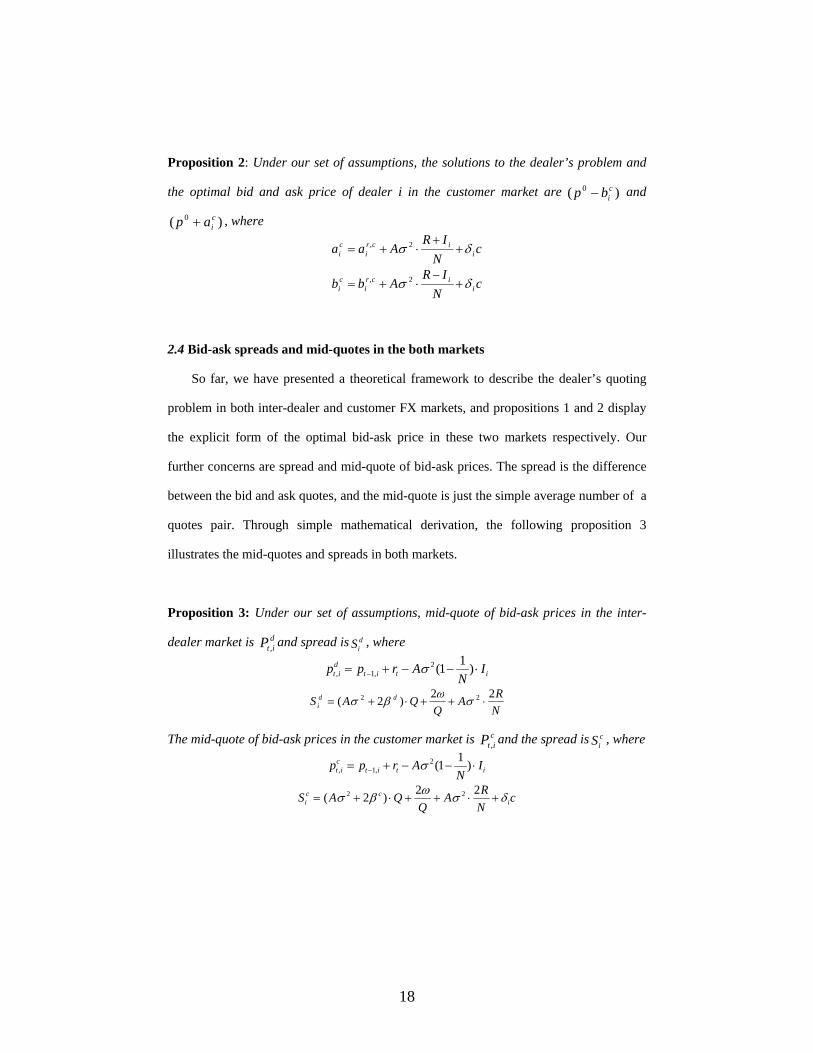
Proposition 2: Under our set of assumptions, the solutions to the dealer’s problem and
the optimal bid and ask price of dealer i in the customer market are and
, where
)( 0 cibp −
)( 0 ciap +
cN
IRAaa i
icri
ci δσ +
+⋅+= 2,
cN
IRAbb i
icri
ci δσ +
−⋅+= 2,
2.4 Bid-ask spreads and mid-quotes in the both markets
So far, we have presented a theoretical framework to describe the dealer’s quoting
problem in both inter-dealer and customer FX markets, and propositions 1 and 2 display
the explicit form of the optimal bid-ask price in these two markets respectively. Our
further concerns are spread and mid-quote of bid-ask prices. The spread is the difference
between the bid and ask quotes, and the mid-quote is just the simple average number of a
quotes pair. Through simple mathematical derivation, the following proposition 3
illustrates the mid-quotes and spreads in both markets.
Proposition 3: Under our set of assumptions, mid-quote of bid-ask prices in the inter-
dealer market is and spread is , where ditP ,
diS
ititd
it IN
Arpp ⋅−−+= − )11(2,1, σ
NRA
QQAS dd
i22)2( 22 ⋅++⋅+= σωβσ
The mid-quote of bid-ask prices in the customer market is and the spread is , where citP ,
ciS
ititc
it IN
Arpp ⋅−−+= − )11(2,1, σ
cNRA
QQAS i
cci δσωβσ +⋅++⋅+=
22)2( 22
18
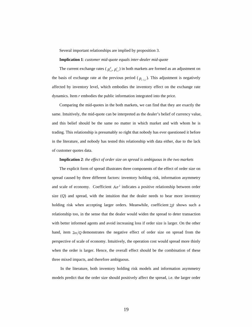
Several important relationships are implied by proposition 3.
Implication 1: customer mid-quote equals inter-dealer mid-quote
The current exchange rates ( ) in both markets are formed as an adjustment on
the basis of exchange rate at the previous period ( ). This adjustment is negatively
affected by inventory level, which embodies the inventory effect on the exchange rate
dynamics. Item r embodies the public information integrated into the price.
cit
dit pp ,, ,
itp ,1−
Comparing the mid-quotes in the both markets, we can find that they are exactly the
same. Intuitively, the mid-quote can be interpreted as the dealer’s belief of currency value,
and this belief should be the same no matter in which market and with whom he is
trading. This relationship is presumably so right that nobody has ever questioned it before
in the literature, and nobody has tested this relationship with data either, due to the lack
of customer quotes data.
Implication 2: the effect of order size on spread is ambiguous in the two markets
The explicit form of spread illustrates three components of the effect of order size on
spread caused by three different factors: inventory holding risk, information asymmetry
and scale of economy. Coefficient indicates a positive relationship between order
size (Q) and spread, with the intuition that the dealer needs to bear more inventory
holding risk when accepting larger orders. Meanwhile, coefficient
2σA
β2 shows such a
relationship too, in the sense that the dealer would widen the spread to deter transaction
with better informed agents and avoid increasing loss if order size is larger. On the other
hand, item Qω2 demonstrates the negative effect of order size on spread from the
perspective of scale of economy. Intuitively, the operation cost would spread more thinly
when the order is larger. Hence, the overall effect should be the combination of these
three mixed impacts, and therefore ambiguous.
In the literature, both inventory holding risk models and information asymmetry
models predict that the order size should positively affect the spread, i.e. the larger order
19
size leads to the wider spread. In contrast, my model shows that the effect is ambiguous.
Empirically, no work has been devoted to testing this relationship before, so we have no
clue about which one is right so far.
Implication 3: customer spread is generally wider than inter-dealer spread, but
their differential decreases with the rise in order size.
To compare the spread in the two markets, the inter-dealer spread is subtracted from
the customer one, and the result is shown in equation (18):
QcSS dci
di
ci ⋅−+=− )(2 ββδ (18)
The first item of the differential )( ciδ says that the customer spread is generally
wider than the inter-dealer one, as the extra cost paid by customers to trade at the best
quote makes the margin possible for the dealer to do so. Moreover, if the dealer wins
customers’ high loyalty, i.e. the value of attractive coefficient iδ is high, he can even
keep a wider customer spread without losing customers, and the difference with the inter-
dealer spread would be bigger. This reflects a fact that in the FX market the dealers
compete with each other not only in the quotes but also in services, and keeping a good
reputation and high customer loyalty is critical to earn higher profit. The coefficient of Q
in equation (18) implies that the difference will decline with the rise in order size, which
results directly from the claim of . Intuitively, with the order size increasing,
information cost of trading with customers is not as much as with dealers, as customers
are usually less informed than the latter.
cd ββ >
In the literature, no formal models have been built to explain this difference, but
there are some indirect evidence just suggesting that customer spread is wider than inter-
dealer one. Yao (1997), for example, found that the customer trades account for only
about 14% of total trading volume, but they represent 75% of the dealer’s total profits.
And also, the market survey by Braas and Bralver (1990) finds that most dealing rooms
generate between 60 and 150 percent of total profits from the customer business. Other
20
than these analyses, neither theoretical model nor empirical testing indicates the
relationship before.
Implication 4: Spreads in both markets are positively affected by exchange rate
volatility
Proposition 3 clearly shows that the spreads in both markets have positive
relationship with exchange rate volatility , i.e. the more volatile the exchange rate is,
the wider the spreads should be. Intuitively, higher volatility of the exchange rate leads
to higher risk of holding the currency, and the dealer would widen the spread to cover the
possibly increasing loss caused by higher market uncertainty. Many models theoretically
show such a relationship in the literature (e.g. Stoll (1978), Ho and Stoll (1981), Black
(1991), Biais (1993), Bollerslev and Melvin (1994), etc). Also, this relationship has been
extensively examined and verified by several persons’ findings. Bessembinder (1994),
Bollerslev and Melvin (1994) as well as Hartmann (1999) all found a positive correlation
between the spread and expected volatility measured by GARCH forecasts. Wei (1994)
regresses the bid-ask spread on the realized exchange rate volatility measured by the
standard deviation of the exchange rate and the anticipated volatility induced from the
price of foreign exchange option respectively, and both regressions agree on the
significant positive relationship between the spread and the volatility. Those findings
provide strong evidence to support the solutions of our model.
2σ
Implication 5: spreads in both markets are negatively related to the number of
dealers
From the proposition, we also can see that the spreads are negatively related to the
number of dealers (N) in both markets, i.e. when more dealers are active in the market,
the spreads will fall. Intuitively, the more dealers quote in the market, the more
competition among them, and one of the efficient strategies to win the competition is to
reduce the spread. In the literature, the competition between dealers and its impact on the
21
spreads have been identified by Stoll (1978) and Biais (1993). Empirically, Huang and
Masulis (1999) used the market data and found that the spreads decrease with a rise in the
number of dealers, which is measured as the frequency of new quotes.
3. Empirical evidence
3.1 Data collection
The data used in this paper were collected from one of the world’s largest online
foreign exchange dealers based in Australia. As the response to each individual
transaction request, the dealer displays the customer and inter-bank rates simultaneously
in its customer rate window1. In order to obtain quotes, a customer first needs to tell the
dealer which currency to sell and the amount of selling (order size). After that, the
customer can submit the transaction request, and the dealer will reveal both customer and
inter-dealer rates for several major currencies associated with this request, as well as the
world time of making these quotes at the very top of the window. To raise the efficiency
of data collecting, we just focused on the rate of the Euro versus the US dollar
(EUR/USD), as it is currently the most traded currency pair in the world.
The dealer’s quotes table actually does not indicate clearly which is bid price and
which is ask, however, we can identify both of them according to their definitions. The
dealer’s bid price of EUR/USD is the rate for the dealer to sell Euro for US Dollar. In
other words, it is the price for a customer to sell US Dollar for Euro. So, when a customer
selects US dollar to sell, the rates of receiving Euro displayed in the quotes table are the
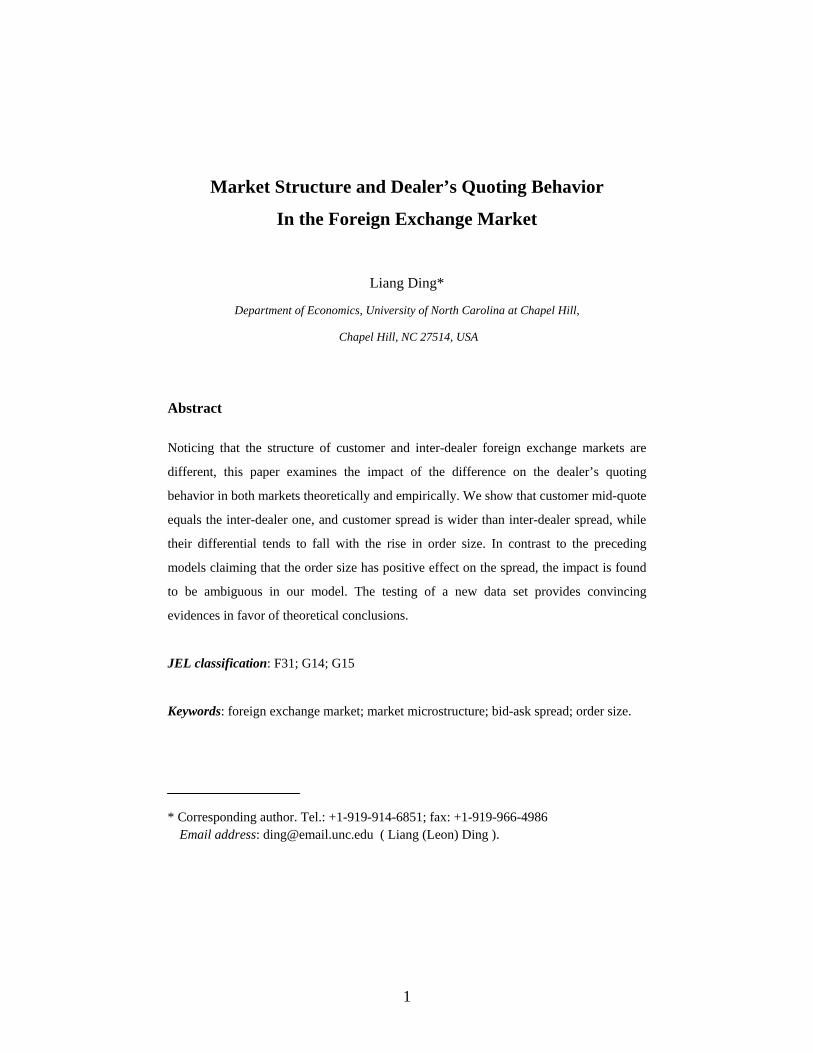
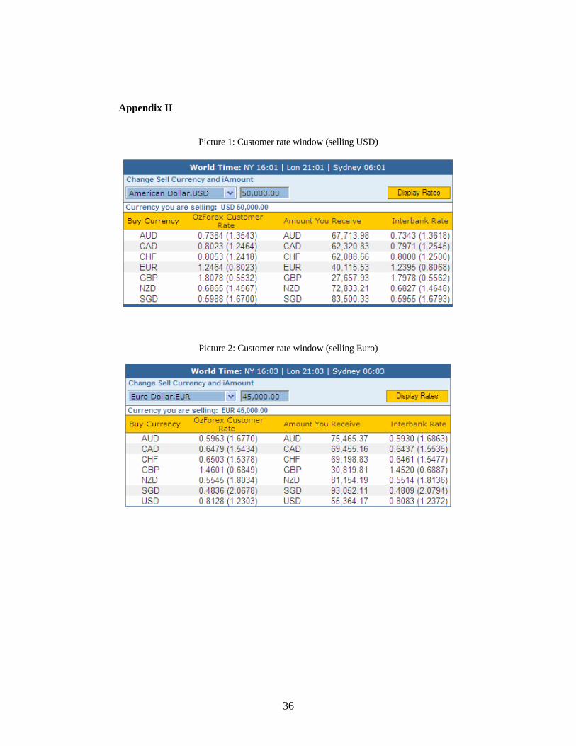
bid prices of EUR/USD. Picture 1, for instance, shows the quotes of selling $50,000 US
dollar at the NY time 16:01 of October 11, 2004. In the row of receiving EUR, we can
find that the customer bid price for EUR/USD is 0.8023, while the inter-bank bid price is
1 Readers can get some clue about what this window looks like from picture 1 and picture 2 attached in appendix II, which are the snap image of this window.
22
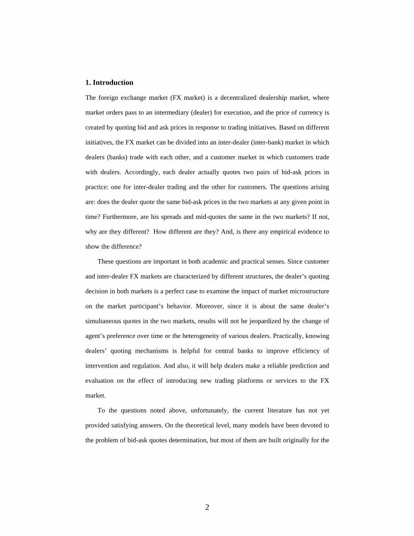
0.8068. The dealer’s ask price of EUR/USD is the rate for the dealer to sell US dollar for
Euro, in other words, it is the price for a customer to sell Euro for US Dollar. If the
customer selects Euro to sell, the rate of receiving US dollar is the ask price of EUR/USD.
Picture 2, for example, shows the quotes for selling 45,000 Euro at the NY time 16:03 of
October 11, 2004, and customer ask price for EUR/USD is 0.8128, while inter-dealer one
is 0.8083.
As described above, bid and ask prices are obtained separately from two quote
windows1, which leads to the question of what amount we should sell in each window to
satisfy the requirement that each pair of bid-ask rates must be associated with the same
order size. Obviously, collecting bid-ask prices by selling the same amount of US dollar
and Euro does not satisfy such a requirement. For example, given the current exchange
rate of EUR/USD is 0.81, selling 50,000 US dollars and 50,000 Euros are two
transactions with unequal order sizes, while selling $50,000 and 45,000 Euros have the
same order size. To make the bid-ask rates correspond to the same request, every time I
collect the data, I converted whatever amount of selling dollar into the equivalent value
of Euro by that day’s prevailing exchange rate as the amount for selling Euro.
Meanwhile, according to our model and many previous works, the bid-ask quotes are
probably affected by the order size. To test whether it is true, bid-ask prices were
collected corresponding to different order sizes, which is changed every five minutes.
The series of order size are generated by a computer program based on the uniform
distribution between $200 and $5,000,000. Meanwhile, in order to obtain reliable
estimation of exchange rate volatility, I update the quotes every minute within the 5-
minute interval for the same order size, so that 5 pairs of bid-ask prices are collected for
one order size.
1 One is selling US dollar to get bid price and the other selling Euro to obtain ask price.
23
The whole process of collecting the data can be described as follows: every five
minutes, take a different number from the random series already created by the computer
as the amount of selling US dollar, and then convert it into the equivalent value of Euro
as the amount of selling Euro. Within the five-minute interval, update the quotes every
minute, while recording all the quotes after the dealer revealed them. This work had been
done during July 5 to July 19, 2004, which covers two weeks and ten work days, the
weekend is excluded due to the low transaction activities. About three hours were spent
each day to do this job (usually 9am—12pm Sydney time, which is supposed to be the
busiest trading time every weekday in the Australian market), and about 1000
observations have been recorded in the data set. During this period, no special events
dramatically changing the market happened, so the data are reliable. Eventually, our data
set consists of the order size of each transaction request, the corresponding customer and
inter-dealer bid-ask prices on the basis of 1-minute interval. Furthermore, the mid-quotes
of bid-ask price and spreads in both markets can be easily obtained by simple
mathematical transformations.
3.2 Features of the data set
Compared to previously used data sets, our data set is characterized by several new
features. First, it contains customer bid-ask quotes rather than just inter-dealer quotes.
Before online foreign exchange dealing services became popular, the customer quotes
were dealers’ commercial secretes and publicly unavailable. Now days, to satisfy the
increasing trading demands around the world and around the clock, the dealer offering
online trading services shows the quotes publicly, which makes it possible to obtain the
data for academic purpose.
Second, in addition to the customer bid-ask quotes, the data set also contains the
inter-dealer quotes, which make the empirical comparison between them possible. In
24
order to do such comparison, the data set should contain bid-ask quotes from both
markets covering the same period and picked at the same frequency, and our data
completely satisfy these requirements.
Third, our data set contains order size corresponding to each customer and inter-
dealer quote, while no previous data set has1. Theoretically, both inventory risk models
and information asymmetry models indicate certain relationship between spread and
single transaction volume, but no empirical work has been done to test this relationship
due to the lack of data.
Finally, in contrast to most of the existing data sets that usually contains daily
variables or less frequency, our data set is characterized by very high frequency
observations. Bid-ask rates in both markets are updated every minute, and order size is
changed every 5 minutes.
Although these new exciting features make our data set very attractive, there are also
a couple of shortcomings related to it. First, both the customer and inter-dealer bid-ask
quotes are not the real transaction rates, but just indicative ones. The dealer publishes the
indicative quotes for customers to make reference for their trade decision, and usually
this type of quotes is slightly different from the rate at which the dealer actually executes
the order. However, our model is built to show the dealer’s optimal quotes without
dealing with the issues of whether the customer or another dealer accepts it or not, or
what the market equilibrium quotes are in the real transaction. Therefore, this
disadvantage will not significantly affect the efficiency of our testing. On the contrary, to
some extent, the data set fits the purpose of our empirical testing very well.
Second, the observations in our data set only cover that part of the trading during
each day’s collecting period, and therefore they are not long continuous time series.
1 Some data sets contain the trading volume, but trading volumes and order size are different concepts: the former is the summation of transaction of quantity no matter sell or buy, while the latter is volume of single transaction.
25
However, according to proposition 3, the spreads are determined by current period
variables, so the testing of our model is more like panel data testing instead of time series.
Therefore, this shortcoming does not affect the efficiency either.
3. 3 Model testing and results
Five implications are indicated based on proposition 3. Among them, the first three
have never been tested before by applying any real market data set, while the other two,
especially the relationship between the spread and the volatility, have been extensively
examined, so our empirical tests will focus on the first three implications.
We first start with the implication 1. Intuitively, the mid-quote of bid-ask prices can
be interpreted as the dealer’s belief of currency value, and this belief should be the same
no matter who he is trading with. Theoretically, no formal model has been built to
illustrate such equality in the literature before, although many people believe so. Our
model describes the dealer’s quoting behavior in both markets respectively, and the mid-
quotes of bid-ask price turn out to be exactly the same. If the intuition and our theoretical
explanation are correct, we expect to see that the two mid-quotes should follow the same
evolvement path.
Mid-quotes in both markets are computed as the average value of bid-ask prices,
which are taken as the original form without any mathematical transformation. Two
series of data will be tested in the both markets: mid-quote at the interval of 1-minute as
well as 5-minute. Table 1 in appendix illustrates the descriptive statistics of both series,
as well as the results of t-test on the difference between them. As we can see from the
table, mean value and standard deviations of customer and inter-dealer mid-quotes are
very close for both series. Meanwhile, t statistics in the tests are very high (21.6599 for 1-
minute series and 7.1929 for 5-minute), so that for neither series can we reject the
hypothesis that they are equal to each other at the significance level of over 99.99%.
26
Furthermore, in order to test whether two mid-quotes are equal to each other exactly,
it is better to regress the following equation (19):
tdt
ct pp εβα +⋅+= (19)
where are customer and inter-dealer mid-quotes respectively dt
ct pp ,
If our analysis is correct, then the null hypothesis that 1,0 == βα should be
accepted in the regression above. However, it is well known that spot exchange rate is an
unstationary process integrated by order 1 (I(1) process). The results of unit root test in
table 2 verify such a judgment. Both Dickey-Fuller and Phillips-Perron tests cannot reject
the null hypothesis of unit root at above 99% significance level. Therefore it might be
inappropriate to regress two series of mid-quotes directly.
To overcome this problem, we regress the first order difference of mid-quotes,
instead of their levels, shown as the following equation (20):
tdt
dt
ct
ct pppp εβα +−+=− ++ )( 11 (20)
Apparently, the null hypothesis that 1,0 == βα should also be accepted, if the
customer mid-quote equals the inter-dealer one. The regression results of both equation
(19) and (20) are summarized in table 3. According to the table, all regressions display
extremely significant results about the coefficients of the equation, and the null
hypothesis is accepted at high significance.
Several figures in the appendix also help show this equality. Figure 1 and 2 are the
two-way scatter plots of customer and inter-dealer mid-quotes at the interval of 5 minutes
and 1 minute respectively. A 45 degree line can be found on each figure, which means
the mid-quotes in the two markets are nearly identical. Figure 3 illustrates the plot of both
mid-quotes at 5-minute intervals across periods, in which an inter-dealer mid-quote is
represented by circle, and each dot stands for customer mid-quote. As shown from the
figure, most dots are surrounded by the circles, which implies that both observations are
at the same position and share the equal value. To show the figure more clearly, I enlarge
27
the part of figure 3 in figure 4, which shows the mid-quotes in both markets during NY
time 19:46—21:26 pm July 15 (Sydney time 9:46—11:26AM July 16). It is obvious that
customer mid-quotes and inter-dealer mid-quotes are equal to each other most of the time,
and are otherwise very close to each other.
Then we move on to the implication 3. According to proposition 3, the differential
between customer spread and inter-dealer spread can be written as:
QcSS dcdc ⋅−+=− )(2 ββδiii (21)
Since equation (21) describes a simple linear relationship, and all variables contained
in the equation are well measured, we just use OLS to test a linear model as below:
(22) εαα +⋅+=− Qss dc10
Variable Q in the equation is measured by logarithm of order size, and spreads in
both markets are represented by the relative spreads, which are computed from customer
and inter-dealer bid-ask prices at the 5-minute interval by the following formula:
)log()log( bas −= (23)
where a and b are ask and bid prices respectively
Based on the analysis in section 2.4, we claim that customer spread is generally
greater than inter-dealer spread, but their differential decreases with a rise in order size. If
this analysis is right, we expect to see a significant positive intercept and a negative
coefficient of order size in the regression. Table 4 first illustrates descriptive statistics
about the two spreads at 5-minute intervals. As we can see, average customer spread
during the data collecting period is 0.013811, and it is significantly higher than the inter-
dealer spread over the same period, which has an average value of only 0.0016051. The
lower part of table 2 reports the regression results. A highly significant positive intercept
is found, implying that the customer spread is in general greater than the inter-dealer one,
28
while significantly negative coefficient of order size says the difference will fall with the
rise in order size. R square and F test results indicate that this regression is very reliable.
Finally, we inspect implication 2. In our analysis before, the effects of order size on
spread in both markets are claimed to be ambiguous. The impact is shown to be a
combination of three components, among which market uncertainty and information
asymmetry cause positive effects, while the scale of economy implies a negative effect.
Meanwhile, the information cost of trading with customers is not as much as with the
dealer given the order size increasing, as we believe customers are usually less informed
than the latter. So, the impact of order size on the customer spread should be less than the
inter-dealer spread. Also, like earlier studies, our model suggests the positive correlation
between the spread and the exchange rate volatility.
In order to test these relationships, the following linear equation (24) will be
regressed in both the inter-dealer and customer FX markets:
(24) εασαα +⋅+⋅+= ttt Qs 22
10
Where Q measures order size and represents exchange rate volatility 2σ
In the above equation, the customer and inter-dealer spreads are also measured as the
logarithm of the ratio of the ask price to the bid price, as shown in equation (23). The
order size is taken as the logarithm of the original observations.
Volatility variable is literally the expected variance of the exchange rate in the
model, but we only have actual variance directly from the data. Many economists agree
that GARCH(1,1) is a proper model to describe the exchange rate variability in the FX
market. So we first estimate GARCH(1,1) by using the series of actual mid-quotes, which
are computed according to the formula below:
2σ
2)log()log( bamidquote +
=
where a, b are ask price and bid price respectively
29
And then predict expected exchange rate volatility by the estimated GARCH model. Thus
the volatility variable is measured as the GARCH(1,1) fitted exchange rate variance
within the 5-minute interval in our empirical testing.
2σ
To show the robustness of the relationships, for each of the two markets, I employ
two series of spread: one is average spread within the 5-minute interval (spread I), and
the other is the spread picked at the beginning of each interval (spread II).
Table 5 summarizes the results of regressing spread on exchange rate volatility and
order size, from which three major conclusions can be drawn. First, in contrast to the
prediction implied by preceding models that order size has a positive effect on spread,
our results provide totally opposite evidence. In the two regressions of customer spread,
the coefficients of order size are both negative numbers with high significance level,
while in the inter-dealer regressions the coefficients seem not to be significantly different
from zero. These results show that the effect of order size on spread is ambiguous, which
is consistent with our prediction. Second, the results show that the coefficient of order
size in the customer regression is about -0.0015, while the inter-dealer one is nearly 0,
which verifies the claim we made before that the impact of order size on the customer
spread should be less than the inter-dealer spread. This result supports our analysis that
inter-dealer transaction is involved with more information cost than customer trading, so
that the dealer tends to widen spread more to deter adverse selection in the inter-dealer
market. Third, surprisingly, volatility does not show significant positive effect on spreads
in all regressions, which has been extensively verified in the literature. The probable
reason is the interval of 5-minute may be too short for the dealer to integrate the volatility
into the quotes.
30
4. Conclusion
To examine the dealer’s quoting behavior under the different market structures, I develop
a model viewing the dealer as a risk aversion agent who optimizes his portfolio by
choosing bid-ask prices. The differences between inter-dealer and customer markets are
recognized and incorporated into the model, and the optimal bid-ask quotes are solved in
both markets, so that the explicit forms of mid-quotes and spreads are obtained for further
analysis.
Our model solutions show that customer mid-quote equals inter-dealer one, which
suggests that mid-quote of the dealer’s bid-ask prices reflects his belief in value of
currency and should be the same in both markets. We also find that customer spread is
wider than inter-dealer spread, which is attributable to the distinction in information
transparency of the two markets. Meanwhile, since dealers are usually better informed
than customers, the dealer is more willing to raise the spread for inter-dealer trading
relative to customer trading to deter adverse selection, so the differential between the two
spreads tends to decrease when order size is rising. And, in contrast with earlier models
claiming that order size has positive effects on the spread, our model predicts that the
impact is ambiguous.
To test the relationship implied by our model, a new data set has been collected from
an online FX dealer based in Australia. This data set contains both inter-dealer and
customer bid-ask quotes as well as order size covering the same period and picked at the
same frequency. By employing the data set, we find convincing evidence supporting our
theoretical conclusion that customer spread is wider than inter-dealer spread while the
difference declines if the order size is larger. Our results also suggest that customer mid-
quote and inter-dealer one are statistically the same variables, which is consistent with
our theoretical prediction. Meanwhile, the impact of order size on spread is found to be
negative in the customer market while no effect is found in the inter-dealer market, which
31
implies that the impact is ambiguous and stands against the conclusions by preceding
models.
Although our work throws some light on the market microstructure of FX markets
and its impact on the dealer’s quoting behavior, it also reveals more open area to be
explored. First, our study only involves one individual dealer and one currency pair.
Whether the conclusions apply to other dealers and other currencies deserves further
work. Second, we did not consider too much heterogeneity of various dealers when we
built the model, while different dealers with various preferences should act differently in
the FX market. How this factor affects their behavior is another important topic for
further research. Finally, IT technology has been progressing rapidly in the past two
decades, which has a huge effect on the FX market. What changes the new trading
platform and services bring to the market participants and how their behavior adjusts in
the new system should be another exciting research objective.
Acknowledgements
The author thanks Stanley Black, Michael Salemi and Patrick Conway for extensive
comments that helped clarify many of the issues contained in the article, and I am
grateful for Bill Parke’s help of the data collection. I also benefit a lot from the talk with
Richard Lyons and Michael Melvin about the FX market microstructure in the 2005 AEA
conference. Many thanks also to the participants in UNC seminars for stimulating
discussions.
32
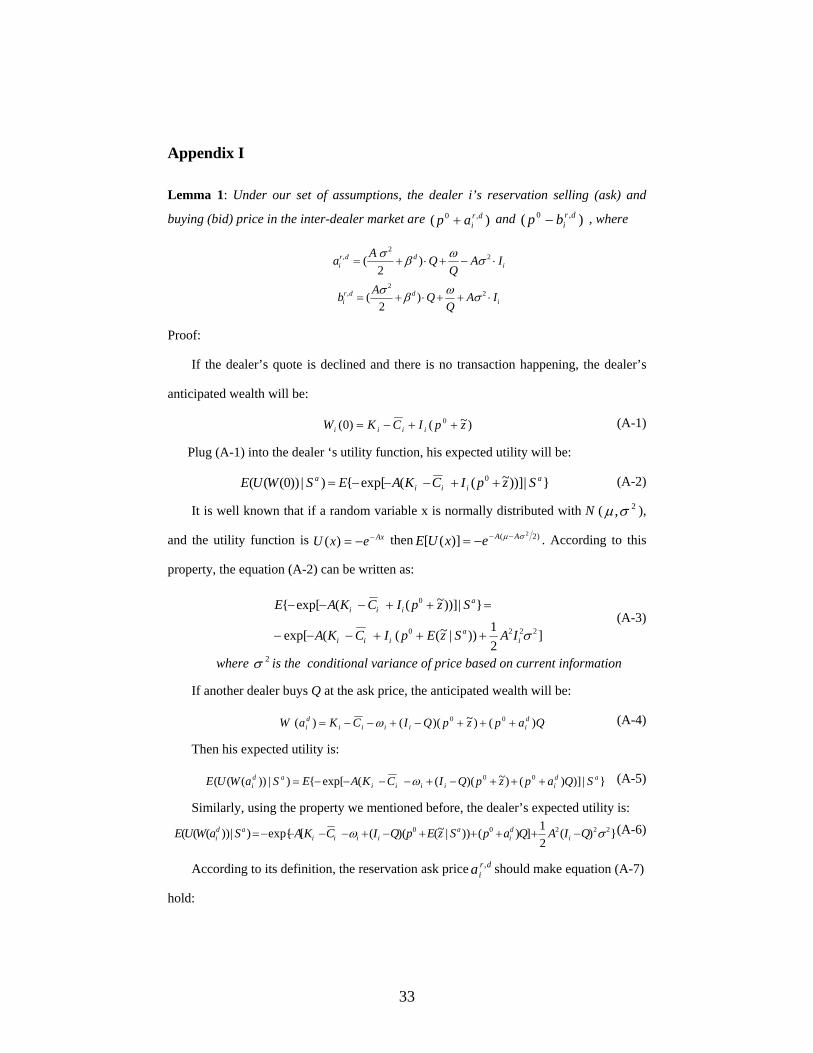
Appendix I Lemma 1: Under our set of assumptions, the dealer i’s reservation selling (ask) and
buying (bid) price in the inter-dealer market are and , where )( ,0 driap + )( ,0 dr
ibp −
iddr
i IAQ
QAa ⋅−+⋅+= 22
, )2
( σωβσ
iddr
i IAQ
QAb ⋅++⋅+= 22
, )2
( σωβσ
Proof:
If the dealer’s quote is declined and there is no transaction happening, the dealer’s
anticipated wealth will be:
)~()0( 0 zpICKW ++−= iiii (A-1)
Plug (A-1) into the dealer ‘s utility function, his expected utility will be:
}|))]~((exp[{)|))0((( 0 aiii
a SzpICKAESWUE ++−−−= (A-2)
It is well known that if a random variable x is normally distributed with N ( ),
and the utility function is then
2,σµ
AxexU −−=)( )2( 2
)]([ σµ AAexUE −−−= . According to this
property, the equation (A-2) can be written as:
]21))|~(((exp[
}|))]~((exp[{
2220
0
σia
iii
aiii
IASzEpICKA
SzpICKAE
+++−−−
=++−−− (A-3)
where is the conditional variance of price based on current information 2σ
If another dealer buys Q at the ask price, the anticipated wealth will be:
QapzpQICKaW dd )() iiiiii~)(()( 00 +++−+−−= ω (A-4)
Then his expected utility is:
}|)])()~)(((exp[{)|))((( 00 adad SQapzpQICKAESaWUE +++−+−−−−= ω iiiiii (A-5)
Similarly, using the property we mentioned before, the dealer’s expected utility is:
})(21])())|~()(([exp{)|))((( 22200 σω QIAQapSzEpQICKASaWUE i
di
aiiii
adi −++++−+−−−−= (A-6)
According to its definition, the reservation ask price should make equation (A-7)
hold:
dria ,
33
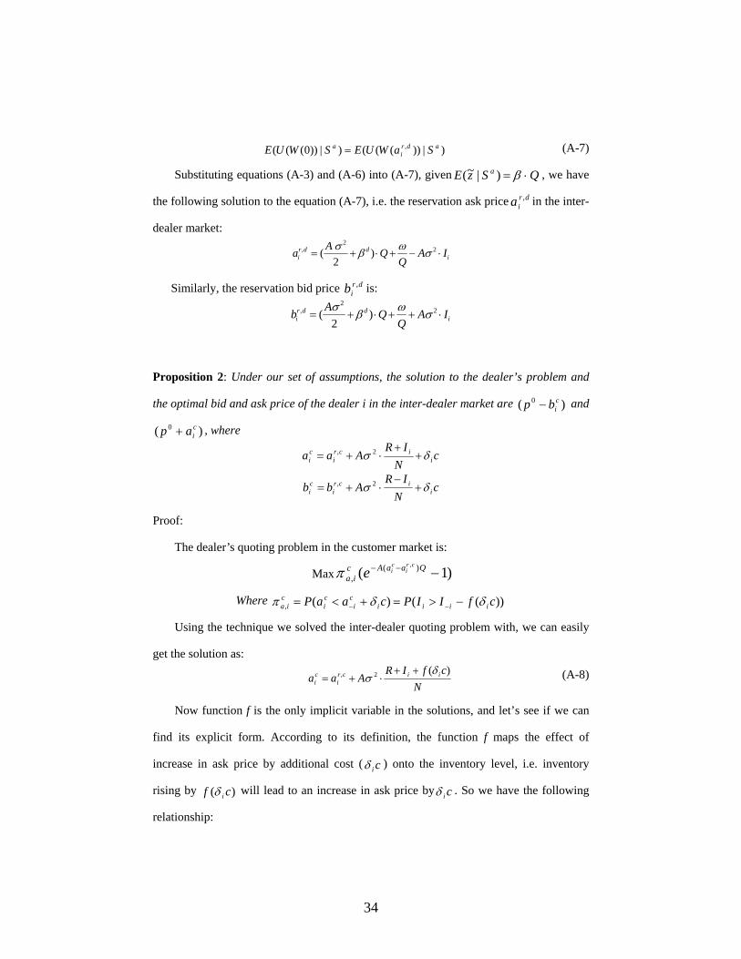
)|))((()|))0((( , adri
a SaWUESWUE = (A-7)
Substituting equations (A-3) and (A-6) into (A-7), given QSzE a ⋅= β)|~( , we have
the following solution to the equation (A-7), i.e. the reservation ask price in the inter-
dealer market:
dria ,
iddr
i IAQ
QAa ⋅−+⋅+= 22
, )2
( σωβσ
Similarly, the reservation bid price is: drib ,
iddr
i IAQ
QAb ⋅++⋅+= 22
, )2
( σωβσ
Proposition 2: Under our set of assumptions, the solution to the dealer’s problem and
the optimal bid and ask price of the dealer i in the inter-dealer market are and
, where
)( 0 cibp −
)( 0 ciap +
cN
IRAaa i
icri
ci δσ +
+⋅+= 2,
cN
IRAbb i
icri
ci δσ +
−⋅+= 2,
Proof:
The dealer’s quoting problem in the customer market is:
Max )1( )(,
,
−−− QaaAcia
cri
cieπ
Where ))(()(, cfIIPcaaP iiiic
ici
cia δδπ −>=+<= −−
Using the technique we solved the inter-dealer quoting problem with, we can easily
get the solution as:
NcfIR
Aaa iicri
ci
)(2, δσ
++⋅+= (A-8)
Now function f is the only implicit variable in the solutions, and let’s see if we can
find its explicit form. According to its definition, the function f maps the effect of
increase in ask price by additional cost ( ciδ ) onto the inventory level, i.e. inventory
rising by )( cf iδ will lead to an increase in ask price by ciδ . So we have the following
relationship:
34
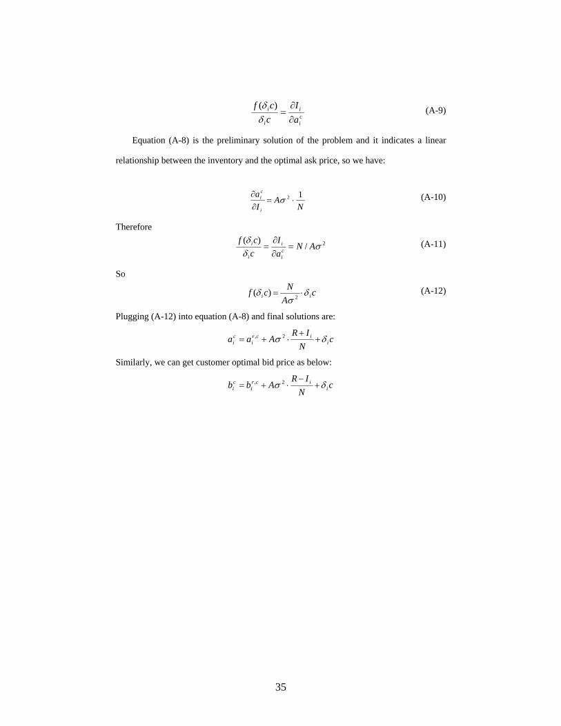
ci
i
i
i
aI
ccf
∂∂
=δδ )( (A-9)
Equation (A-8) is the preliminary solution of the problem and it indicates a linear
relationship between the inventory and the optimal ask price, so we have:
NA
Ia
i
ci 12 ⋅=
∂∂
σ (A-10)
Therefore
2/)(
σδδ
ANaI
ccf
ci
i
i
i =∂∂
= (A-11)
So
cA
Ncf ii δσ
δ ⋅= 2)( (A-12)
Plugging (A-12) into equation (A-8) and final solutions are:
cN
IRAaa i
icri
ci δσ +
+⋅+= 2,
Similarly, we can get customer optimal bid price as below:
cN
IRAbb i
icri
ci δσ +
−⋅+= 2,
35
Appendix II
Picture 1: Customer rate window (selling USD)
Picture 2: Customer rate window (selling Euro)
36
References:
Bessembinder, Hendrik, 1994. Bid-ask spreads in the interbank foreign exchange markets.
Journal of Financial Economics, 35(3), pp. 317-348.
Biais, Bruno, 1993. Price Formation and Equilibrium liquidity in fragmented and
centralized markets. Journal of Finance Vol 484, No.1 157—185
Black, Stanley W., 1991. Transactions costs and vehicle currencies. Journal of
International Money and Finance, Elsevier, vol. 10(4), pages 512-526, 12
Bollerslev, Tim and I Domowitz 1993. Trading patterns and prices in the interbank
foreign exchange market. Journal of Finance, 48, pp. 1421-43.
Bollerslev, Tim & Melvin, Michael, 1994. Bid--ask spreads and volatility in the foreign
exchange market: An empirical analysis, Journal of International Economics,
Elsevier, vol. 36(3), pages 355-372, 5.
Braas, Alberic and Charles B. Bralver, 1990, An analysis of trading profits: How most
tradingrooms really make money? Journal of Applied Corporate Finance, Winter,
Vol. 2, No. 4.
Demos, Antonis A.; Goodhart, Charles A. E., 1996. The Interaction between the
Frequency of Market Quotations, Spread and Volatility in the Foreign Exchange
Markets, Applied Economics, March v. 28, iss. 3, pp. 377-86
Evans, M., Lyons, R., 2002. Order flow and exchange-rate dynamics. Journal of Political
Economy 110, 170-180.
Garman, Mark B., 1978. The Pricing of Supershares. Journal of Financial Economics,
March 1978, v. 6, iss. 1, pp. 3-10
Glassman Debra, 1987. Exchange Rate Risk and Transactions Costs: Evidence from Bid-
Ask Spreads. Journal of International Money and Finance, Vol. 6, 1987, 479-490.
37
Hartmann, Philipp, 1998.
Journal of International Money and Finance, October, v. 17, iss. 5,
pp. 757-84
Do Reuters Spreads Reflect Currencies' Differences in Global
Trading Activity?
Hartmann, Philipp, 1999. Trading volumes and transaction costs in the foreign exchange
market. Journal of Banking and Finance, Vol. 23, pp. 801-824.
Ho, T., and H. Stoll, 1981. Optimal dealer pricing under transactions and return
uncertainty. Journal of Financial Economics, 9, 47-73.
Huang. D Roger. and Ronald W. Masulis, 1999. FX spread and dealer competition
across the 24-Hour trading day. The Review of Financial Studies. Vol 12 No. 1 61—
93
Jorion, Philippe, 1996. Risk and Turnover in the Foreign Exchange Market. The
microstructure of foreign exchange markets, pp. 19-37, National Bureau of
Economic Research Conference Report series. Chicago and London: University of
Chicago Press,
Laux, Paul A., 1995. Dealer Market Structure, Outside Competition, and the Bid-Ask
Spread. Journal of Economic Dynamics and Control, May 1995, v. 19, iss. 4, pp.
683-710
Stoll, Hans R., 1978. The Supply of Dealer Services in Securities Markets. Journal of
Finance Sept. 1978, v. 33, iss. 4, pp. 1133-51
Wei, Shang-Jin, 1994. Anticipations of Foreign Exchange Volatility and Bid-Ask
Spreads. National Bureau of Economic Research Working Paper: 4737
Yao, J. 1998. Market making in the inter-bank foreign exchange market, New York
University Salomon Center Working Paper #S-98-3.
38
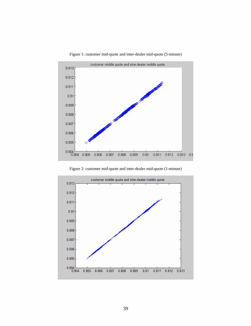
Figure 1: customer mid-quote and inter-dealer mid-quote (5-minute)
Figure 2: customer mid-quote and inter-dealer mid-quote (1-minute)
39
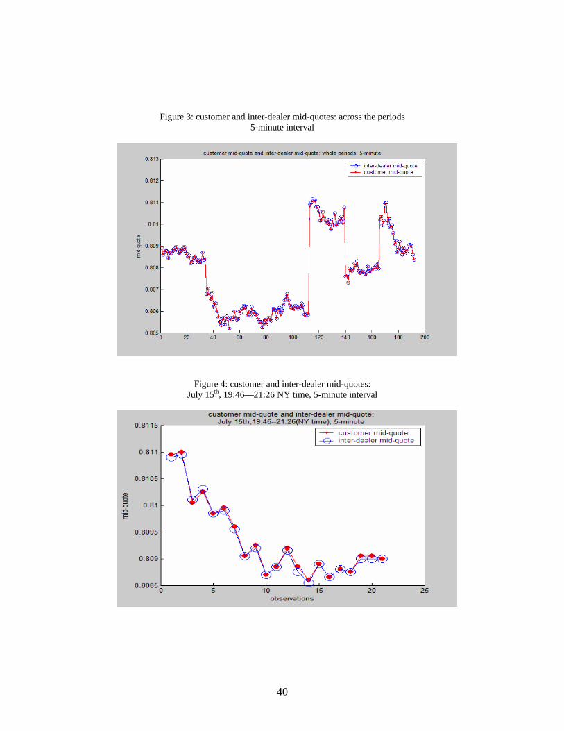
Figure 3: customer and inter-dealer mid-quotes: across the periods
5-minute interval
Figure 4: customer and inter-dealer mid-quotes: July 15th, 19:46—21:26 NY time, 5-minute interval
40
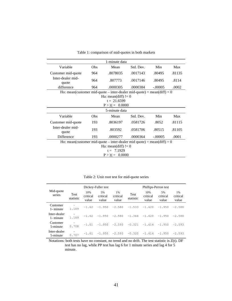
Table 1: comparison of mid-quotes in both markets
1-minute data Variable Obs Mean Std. Dev. Min Max
Customer mid-quote 964 .8078035 .0017143 .80495 .81135 Inter-dealer mid-
quote 964 .807773 .0017146 .80495 .8114
difference 964 .0000305 .0000384 -.00005 .0002 Ho: mean(customer mid-quote – inter-dealer mid-quote) = mean(diff) = 0
Ha: mean(diff) != 0 t = 21.6599
P > |t| = 0.0000 5-minute data
Variable Obs Mean Std. Dev. Min Max Customer mid-quote 193 .8036197 .0581726 .8052 .81115
Inter-dealer mid-quote 193 .803592 .0581706 .80515 .81105
Difference 193 .0000277 .0000364 -.00005 .0001 Ho: mean(customer mid-quote – inter-dealer mid quote) = mean(diff) = 0
Ha: mean(diff) != 0 t = 7.1929
P > |t| = 0.0000
Table 2: Unit root test for mid-quote series
Dickey-Fuller test Phillips-Perron test Mid-quote
series Test statistic
10% critical value
5% critical value
1% critical value
Test statistic
10% critical value
5% critical value
1% critical value
Customer 1- minute
-1.189 -1.62 -1.950 -2.580 -1.533 -1.620 -1.950 -2.580
Inter-dealer 1- minute
-1.189 -1.62 -1.950 -2.580 -1.364 -1.620 -1.950 -2.580
Customer 5-minute
-0.708 -1.61 -1.950 -2.593 -0.321 -1.614 -1.950 -2.593
Inter-dealer 5-minute
-0.707 -1.61 -1.950 -2.593 -0.320 -1.614 -1.950 -2.593
Notations: both tests have no constant, no trend and no drift. The test statistic is Z(t). DF test has no lag, while PP test has lag 6 for 1 minute series and lag 4 for 5 minute.
41
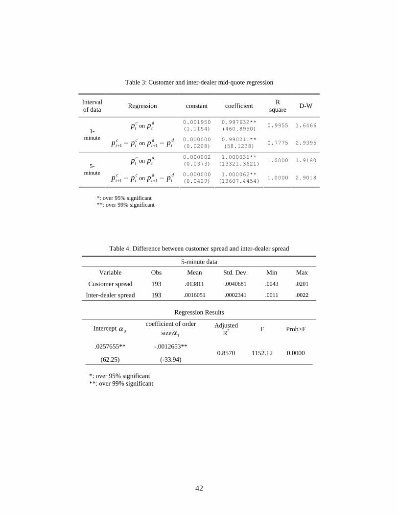
Table 3: Customer and inter-dealer mid-quote regression
Interval of data Regression constant coefficient R
square D-W
ctp on d
tp 0.001950(1.1154)
0.997632** (460.8950) 0.9955 1.6466
1-minute c
tct pp −+1 on d
tdt pp −+1
0.000000(0.0208)
0.990211** (58.1238) 0.7775 2.9395
ctp on d
tp 0.000002(0.0373)
1.000036** (13321.3621) 1.0000 1.9180
5-minute c
tct pp −+1 on d
tdt pp −+1
0.000000(0.0429)
1.000062** (13607.4454) 1.0000 2.9018
*: over 95% significant **: over 99% significant
Table 4: Difference between customer spread and inter-dealer spread
5-minute data
Variable Obs Mean Std. Dev. Min Max
Customer spread 193 .013811 .0040681 .0043 .0201
Inter-dealer spread 193 .0016051 .0002341 .0011 .0022
Regression Results
Intercept coefficient of order
size0α1α
Adjusted R2 F Prob>F
.0257655**
(62.25)
-.0012653**
(-33.94) 0.8570 1152.12 0.0000
*: over 95% significant **: over 99% significant
42
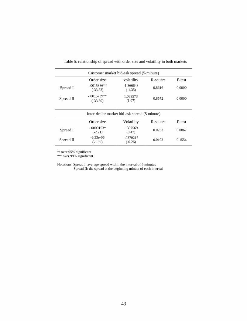
Table 5: relationship of spread with order size and volatility in both markets
Customer market bid-ask spread (5-minute)
Order size volatility R-square F-test
Spread I -.0015836** (-33.82)
-1.366648 (-1.35) 0.8616 0.0000
Spread II -.0015739** (-33.60)
1.089573 (1.07) 0.8572 0.0000
Inter-dealer market bid-ask spread (5 minute)
Order size Volatility R-square F-test
Spread I -.0000153* (-2.21)
.1397569 (0.47) 0.0253 0.0867
Spread II -6.33e-06 (-1.89)
-.0370215 (-0.26) 0.0193 0.1554
*: over 95% significant **: over 99% significant Notations: Spread I: average spread within the interval of 5 minutes Spread II: the spread at the beginning minute of each interval
43
Recommended