Market Maker Revenues and Stock Market Liquidity
Carole Comerton-Forde Terrence Hendershott
Charles M. Jones*
August 13, 2007
* Comerton-Forde is at University of Sydney ([email protected]); Hendershott is at Haas
School of Business, University of California, Berkeley ([email protected]); and Jones is at Columbia Business School ([email protected]). We thank the NYSE for providing data. We thank Ekkehart Boehmer, Joel Hasbrouck, Jerry Liu, Pam Moulton, and participants at the NBER Market Microstructure meeting, Columbia, and Maryland for helpful comments. Hendershott gratefully acknowledges support from the National Science Foundation. Part of this research was conducted while Comerton-Forde and Hendershott were visiting economists at the New York Stock Exchange.
Market Maker Revenues and Stock Market Liquidity
Abstract
We use an 11-year panel of daily specialist revenues on individual NYSE stocks to explore the relationship between market-maker revenues and liquidity. If market makers suffer substantial trading losses, lenders may respond by increasing funding costs or reducing credit lines, and market makers should respond by reducing liquidity provision. The data indicate that when specialists in aggregate lose money on their inventories, market-wide effective spreads widen in the days or weeks that follow, even after controlling for stock returns, volatility, and volume. This suggests an important role for market-maker financial performance in explaining liquidity time-variation. Revenues at the specialist firm level explain liquidity changes in that firm’s assigned stocks. Revenues at the individual stock level do not explain changes in individual stock liquidity, consistent with a financial constraints model with broadly diversified intermediaries. Aggregate specialist revenues are increasing in conditional return volatility, as is revenue volatility. Specialist margins (specialist revenue per dollar of trading volume) are essentially constant across stocks, implying limited scope for cross-subsidization.
1. Introduction
Liquidity is important for our understanding of how traders and institutions affect asset
prices (Amihud, Mendelson, and Pedersen (2006)). Theoretical work by Gromb and Vayanos
(2002) and Brunnermeier and Pedersen (2006), among others, postulates that limited market
maker capital can explain various empirical features of asset market liquidity. Data limitations
have hampered empirical work in this area, making it difficult to demonstrate strong links
between liquidity supplier behavior and capital constraints. In this paper we use 11 years of New
York Stock Exchange (NYSE) specialist trading revenue data to examine how market maker
revenues impact daily stock market liquidity. The basic mechanism is simple: if market makers
suffer substantial trading losses, lenders may respond by increasing funding costs or reducing
credit lines. All else equal, market makers should respond to these constraints by reducing the
amount of liquidity they are willing to provide.
Hendershott, Moulton, and Seasholes (2007) show that aggregate NYSE specialist positions
are net long over 94 percent of the time. Specialists also have an affirmative obligation to buffer
order flow, buying when others want to sell and vice versa. This means that specialists tend to
lose money when the aggregate market declines. If these losses impose financial constraints on
market makers, then liquidity will be worse immediately thereafter. Thus, market maker trading
losses might be able to account for the well-known negative relationship between liquidity and
lagged returns (see, for example, Chordia, Roll, and Subrahmanyam (2001), Chordia, Sarkar, and
Subrahmanyam (2005), and Hameed, Kang, and Vishwanathan (2006)).
Our data cover only one market maker per stock – the specialist assigned by the NYSE to
that stock – but that liquidity provider is probably the most important one, given the structural
advantages that accrue to the specialist. In addition, specialist revenues may be good proxies for
trading revenues earned by other competing liquidity suppliers, such as market-makers on
regional exchanges, proprietary trading desks at various Wall Street firms, hedge funds
following a market-making strategy, and so on. While we have no direct evidence that these
other market makers have a long bias, an average long position might be optimal in the presence
of an equity premium. In any case, all of these market-makers buffer order flow, so all are likely
to lose money following a sharp price decline. Thus, it may be appropriate to think of our
specialist revenue numbers as reflective of broader market-maker revenues.
1
Specialist trading revenues vary considerably over time. In fact, specialists in aggregate lose
money on about 10% of the trading days during our sample, the average loss is about $4 million
on these days, and these losses tend to cluster together in time. So there is ample scope for
negative specialist revenues to force contractions in liquidity provision. Specialists almost
always earn positive trading revenue on short-term roundtrip transactions, but are exposed to the
possibility of losses on inventories held for longer periods. This suggests that the revenues
associated with longer-term inventories could be better indicators of whether financial
constraints are easing or tightening. When we decompose revenues into intraday vs. longer-term
components, we find that revenues associated with inventories held overnight are indeed the
ones that are associated with future liquidity. This overnight breakpoint dovetails nicely with
our story, because anecdotal evidence indicates that lenders and risk managers are most likely to
evaluate financing terms and position limits based on daily P&L and end-of-day balance sheets.
Because of the long bias in their aggregate position, specialists as a group tend to lose more
money when the market falls. We already know that when the market falls, aggregate liquidity
worsens. Putting these two facts together, we would expect to see in univariate regressions that
liquidity worsens when specialists lose money. Given this collinearity, the empirical challenge
is to separate the two variables and assess whether market maker revenues can account for the
observed time-series predictability in liquidity. Fortunately, aggregate specialist trading
revenues are not perfectly correlated with contemporaneous market returns, so it is possible to
find times when specialists lose money without a corresponding market fall, or when specialists
earn positive trading revenue in a declining market. When both variables appear in a predictive
regression, specialist losses are associated with wider spreads next period. At daily horizons,
market declines also have incremental explanatory power, but market returns are no longer
significant at weekly horizons. So it appears that this proxy for financial constraints is able to
completely explain weekly variation in aggregate liquidity, but is unable to completely account
for higher-frequency liquidity squiggles.
The effects are strong at the aggregate level. However, if specialist financing constraints are
the mechanism and specialist firms do not all lose money at the same time, the relationship
should be present and in fact stronger at the specialist firm level. There should be a common
component in liquidity for all stocks assigned to a particular specialist firm, and that firm’s
revenues should affect liquidity in those stocks. Coughenour and Saad (2004) demonstrate the
2
former; here we show that a specialist firm’s trading revenues predict future liquidity in that
firm’s assigned stocks.
Finally, at the individual stock level, there is also substantial time-series variation in
liquidity. But as long as individual equity markets are not segmented and market-makers are
broadly diversified, market-maker losses that are confined to a single stock should not affect the
market-maker’s ability to provide liquidity in that stock. And that is exactly what we find. The
financing constraints seem to be operating at the specialist firm level and at an aggregate market-
wide level.
Because aggregate specialist revenues are important for liquidity, we investigate the sources
of revenue variation through time. Aggregate return volatility turns out to matter most, and
volatility has the biggest impact on the intraday component of revenues. Because this intraday
component is really bid-ask spreads less losses to more informed traders, either spreads earned
by specialists are wider in volatile markets, or specialists are better able to sidestep informed
trades in volatile markets. Either way, it appears that specialist market power is greater when
return variance is high.
The remainder of the paper is organized as follows. Section 2 reviews related literature.
Section 3 provides a general description of our data and sample. Section 4 shows the basic
relation between aggregate market maker revenues and market liquidity. Section 5 looks at the
specialist firm level; Section 6 examines individual stock liquidity and market maker revenues.
Section 7 investigates the time series of market maker revenues and their volatility. Section 8
studies the cross section of individual stock market maker revenues and revenues per dollar
traded. Section 9 concludes.
2. Related Literature
Most models of market liquidity focus on three types of trading costs: fixed, inventory, and
information.1 Theory focusing on funding costs (capital constraints) is more recent. Kyle and
Xiong (2001) show how convergence traders (arbitrageurs) having decreasing risk aversion leads
to correlated liquidations and higher volatility. Gromb and Vayanos (2002) study a model in
1 Kyle (1985) and Gloston and Milgrom (1985) examine the impact of private information. Stoll (1978), Amihud
and Mendelson (1980), Ho and Stoll (1981, 1983), and Grossman and Miller (1988) examine the impact of inventories.
3
which arbitrageurs face margin constraints and show how these arbitrageurs' liquidity provision
benefits all investors.2 However, because the arbitrageurs cannot capture all of the benefits, they
fail to take the socially optimal level of risk. Weill (2006) examines dynamic liquidity provision
by market makers and shows that if they have access to sufficient capital, the market makers
provide the socially optimal amount of liquidity, but if capital is insufficient or too costly then
market makers will undersupply liquidity. Brunnermeier and Pedersen (2006) construct a
model—along the lines of Grossman and Miller (1988)—that also links market makers’ funding
and market liquidity.3
Chordia, Roll, and Subrahmanyam (2001) are the first to show that volatility and negative
returns reduce aggregate stock market liquidity. Chordia, Roll, and Subrahmanyam (2000) and
Hasbrouck and Seppi (2001) examine the common component in liquidity changes across stocks.
Coughenour and Saad (2004) study this further by showing that the co-movement in liquidity is
stronger among stocks traded by the same NYSE specialist firm and this commonality is stronger
for smaller specialist firms. Hameed, Kang, and Viswanathan (2006) examine the impact of
negative returns on liquidity commonality and co-movement. Chordia, Sarkar, and
Subrahmanyam (2005) study linkages between order flows, volatility, returns, and liquidity
across the stock and bond markets.
Both liquidity supplier wealth and the amount of capital committed by liquidity suppliers
play significant roles in the theoretical work on capital constraints and liquidity. This paper
examines how market-maker firms’ gains and losses, which should correlate with their wealth,
impacts liquidity. Using specialist inventory positions, Hendershott, Moulton, and Seasholes
(2007) show that the inventory (committed capital) channel is also important for aggregate
liquidity.4 They show that larger specialist inventories imply worse liquidity, and that specialists
take on less inventory when liquidity worsens.
2 Yuan (2005) provides a model which shows a link between information asymmetry and liquidity when informed
investors are constrained. 3 This effect is more severe if market makers face market-liquidity-reducing predation (Attari, Mello, and Ruckes
(2005) and Brunnermeier and Pedersen (2005)). 4 Naik and Yadav (2003) show that the contemporaneous relationship between government bond price changes
and changes in market-maker inventories differs when market-maker inventories are very long or very short, but they do not directly examine liquidity.
4
A number of papers examine the profitability of specialists.5 Hasbrouck and Sofianos (1993)
decompose specialist profits by trading horizon and find that most profits are due to their high
frequency (short-term) trading strategies. Coughenour and Harris (2004) extend this
econometrically and examine how the tick size change from 1/16 to $0.01 impacts specialist
profits. Panayides (2006) analyzes how specialists’ trading, inventory, and profitability depend
on their obligations under NYSE rules.
3. Data and Descriptive Statistics
Three data sets are used in our empirical work. CRSP is used to identify firms (permno),
market capitalization, closing prices, returns, and trading volume. Market-wide returns are
calculated as the market-capitalization weighted average across stocks. Internal NYSE data
from the specialist summary file (SPETS) provide the specialist inventory position, specialist
purchases, and specialist sales in shares and dollars for each stock each day from 1994 through
2004. The Trades and Quotes (TAQ) master file provides the CUSIP number that corresponds to
the symbol in TAQ on each date and is used to match with the NCUSIP in the CRSP data.6 We
consider only common stocks (SHRCLS = 10 or 11 in CRSP), and we exclude stocks priced over
$500. We use only NYSE trades and quotes from TAQ to calculate liquidity measures.
For each stock each day, we measure the specialist’s gross revenues from trading. These
are gross revenues because we do not subtract any costs, such as salaries, fees, or technology
investments, and they are gross trading revenues because we ignore other possible specialist
revenue sources, mainly brokerage commissions charged to other floor participants.
Gross trading revenues (GTR) in stock i on day t are calculated as in Sofianos (1995) by
marking to market the specialist’s starting and ending inventories and adding the gross profits
due to buys and sells:
)()( 1,1, −−−+−= titiititititit IpIpBSGTR ,
where pit is the share price of stock i at the end of day t, Iit is the specialist’s inventory in shares
of stock i at the end of day t, Sit is the total dollar value of stock i sold on day t, and Bit is the total 5 Market maker profits have been examined in other markets. For example, Hansch, Naik, and Viswanathan
(1999) examine how London Stock Exchange market maker trading profits vary depending on whether the trade is preferenced or internalized.
6 The symbol in TAQ and ticker in CRSP match only 90% of time in our CUSIP matched sample, suggesting that using the TAQ master file to obtain CUSIPs is constructive.
5

dollar value of shares bought. For simplicity we suppress subscripts i in the discussion that
follows.
To decompose these profits, begin by defining stp as the specialist’s average selling price
on day t, with btp the corresponding average buying price, and define st and bt to be the shares
sold and bought, respectively, on day t. Then:
St = st stp
Bt = bt btp .
Now rewrite gross trading revenue as:
)()()( 111 −−− −+−+−= ttttttb
ts
tt ppIIIppbpsGTR tt
and expand the first term in parentheses:
)()()()())(,min( 111 −−−++ −+−+−−−+−= tttttttt
btt
sbsttt ppIIIpsbpbspppbsGTR tttt .
Finally, using the fact that
It = It-1 + (bt – st)
we obtain:
)())(())(())(,min( 11 −−++ −+−−+−−+−= tttttt
stt
bt
bsttt ppIbsppsbppppbsGTR tttt
The first term of this equation captures the difference in buying and selling prices for all round-
trip transactions that the specialist completes on day t, and we call this realized or round-trip
trading revenue RTRt:
))(,min( bsttt tt ppbsRTR −= .
The remaining terms are defined as inventory-related trading revenue ITRt:
)())(())(( 11 −−++ −+−−+−−= tttttt
stt
btt ppIbsppsbppITR tt .
The first two terms of ITR reflect the mark-to-market profits on day t’s changes in inventory
(either long or short), and the last term is the mark-to-market profit on the starting inventory
position. Thus, we have decomposed daily specialist profits for each stock into:
GTRt = RTRt + ITRt,
reflecting an intraday spread-related component and an multi-day inventory-related component.
The weekly GTR, RTR, and ITR are summations of the respective daily variables over five
trading days.
6
To calculate aggregate market maker revenues each day GTR, RTR, and ITR are summed
across all the stocks in the sample. Specialist participation rates and the nature of specialist
trading change markedly when the minimum tick size changes from eighths to sixteenths on June
24, 1997 and from sixteenths to pennies on January 29, 2001.7 Specialist participation also
changes markedly at the beginning of 2003.8 To adjust for these discontinuities, we calculate the
time-series mean of daily specialist revenues in each of four regimes – one for each minimum
tick, plus an additional breakpoint at January 1, 2003 – and adjust our aggregate revenue
measures by the appropriate regime mean.
To measure liquidity at the market level, we construct a daily spread measure averaged
across all stocks in the sample. Because specialists and floor brokers are sometimes willing to
trade at prices within the quoted bid and ask, we use the effective spread rather than the quoted
spread to measure liquidity. The effective spread is the difference between an estimate of the
true value of the security (the midpoint of the bid and ask) and the actual transaction price.9 For
the kth trade in stock j on day t , the dollar effective spread (Ejkt) and the proportional effective
spread (ejkt) are defined as:
Ejkt = 2 Ijkt (Pjkt – Mjkt),
ejkt = 2 Ijkt (Pjkt – Mjkt) / Mjkt.
where Ijkt is an indicator variable that equals one for buyer-initiated trades and negative one for
seller-initiated trades, Pjkt is the trade price, and Mjkt is the quote midpoint prevailing at the time
of the trade. We follow the standard trade-signing approach of Lee and Ready (1991) and, due to
reporting lags, the prevailing quote is taken to be the quote in effect five seconds prior to a trade
for data up through 1998. After 1998, we use contemporaneous quotes to sign trades and
calculate effective spreads (see Bessembinder (2003), for example). We calculate Ejt and ejt, the
mean dollar and proportional effective spreads for each stock each day, by averaging Ejkt or ejkt
7 Though the NYSE moves approximately 100 common stocks to decimals between September and December
2000 as part of its testing and roll-out plans, the vast majority of stocks make the switch on January 29, 2001. 8 In early 2003, the NYSE and SEC begin to investigate the trading behavior of specialists, leading to criminal
indictments of individual specialists and fines for specialist firms (Ip and Craig (2003)). 9 Other liquidity measures such as quoted spreads give qualitatively similar results. Results in this paper also hold
for each of the tick-size sub-periods (eighths, sixteenths, and decimals).
7
using share volume weights, and we calculate the market-wide liquidity measures Et and et as the
cross-sectional mean of Ejt or ejt using market cap weights. We also estimate a number of
specifications at weekly frequencies. For those, we simply calculate an equally-weighted
average of the five daily market-wide effective spreads.
[ Insert Figure 1 Here]
Chordia, Roll, and Subrahmanyam (2001) and Jones (2005) document a downward trend in
average effective spreads over the first half of our sample period. Figure 1 shows that effective
spreads continue this narrowing trend over the rest of the sample, but the decline is interrupted
by the 2000-2002 market decline and punctuated by sharp spread declines around the two
minimum tick size reductions: from eighths to sixteenths in June 1997, and from sixteenths to
pennies in January 2001. To deal with these non-stationarities, we focus on spreads relative to
their average values in the recent past, defining the market-wide relative effective spread est as:
∑=
−−=10
651
ssttt EEes ,
with an analogous definition for esprt, the market-wide relative proportional effective spread.
Lags 6 through 10 are used for the moving average because many of our specifications
predict future effective spreads using returns and volume at lags 1 through 5 as explanatory
variables. Thus, to simplify the interpretation of the results we want to ensure that our effective
spread measure is not affected by contemporaneous correlation between, say, spreads and
returns.
To measure changes in volatility we estimate the asymmetric GARCH(1,1) model of
Glosten, Jagannathan, and Runkle (1993) on daily or weekly aggregate log stock returns Rt:
12
12
11 −−−− +++= ttttt Iuuhh φαδκ ,
where ut = Rt – µ is distributed N(0, ht), and It-1 = 1 if ut-1 ≥ 0 and It-1 = 0 otherwise. In order to
match the treatment of effective spreads, we do not use ht directly as an explanatory variable but
instead define vrett as ht less the average conditional variance ht at lags 6 through 10. In some
regressions we also include uvrett, the unexpected volatility at time t, which is defi s ned a
tt hu −2 .
8
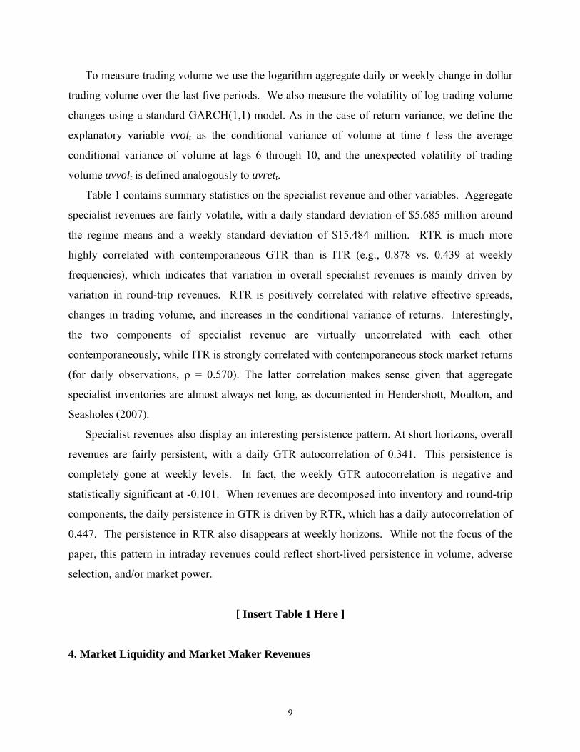
To measure trading volume we use the logarithm aggregate daily or weekly change in dollar
trading volume over the last five periods. We also measure the volatility of log trading volume
changes using a standard GARCH(1,1) model. As in the case of return variance, we define the
explanatory variable vvolt as the conditional variance of volume at time t less the average
conditional variance of volume at lags 6 through 10, and the unexpected volatility of trading
volume uvvolt is defined analogously to uvrett.
Table 1 contains summary statistics on the specialist revenue and other variables. Aggregate
specialist revenues are fairly volatile, with a daily standard deviation of $5.685 million around
the regime means and a weekly standard deviation of $15.484 million. RTR is much more
highly correlated with contemporaneous GTR than is ITR (e.g., 0.878 vs. 0.439 at weekly
frequencies), which indicates that variation in overall specialist revenues is mainly driven by
variation in round-trip revenues. RTR is positively correlated with relative effective spreads,
changes in trading volume, and increases in the conditional variance of returns. Interestingly,
the two components of specialist revenue are virtually uncorrelated with each other
contemporaneously, while ITR is strongly correlated with contemporaneous stock market returns
(for daily observations, ρ = 0.570). The latter correlation makes sense given that aggregate
specialist inventories are almost always net long, as documented in Hendershott, Moulton, and
Seasholes (2007).
Specialist revenues also display an interesting persistence pattern. At short horizons, overall
revenues are fairly persistent, with a daily GTR autocorrelation of 0.341. This persistence is
completely gone at weekly levels. In fact, the weekly GTR autocorrelation is negative and
statistically significant at -0.101. When revenues are decomposed into inventory and round-trip
components, the daily persistence in GTR is driven by RTR, which has a daily autocorrelation of
0.447. The persistence in RTR also disappears at weekly horizons. While not the focus of the
paper, this pattern in intraday revenues could reflect short-lived persistence in volume, adverse
selection, and/or market power.
[ Insert Table 1 Here ]
4. Market Liquidity and Market Maker Revenues
9
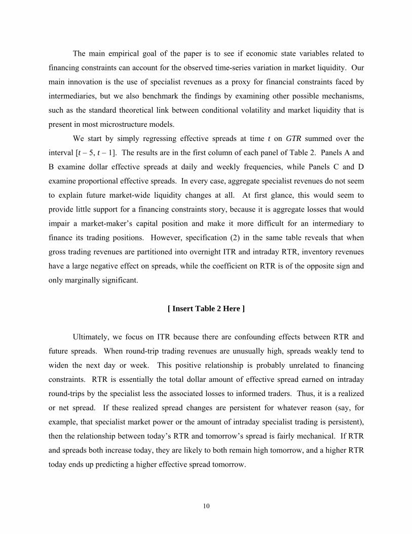
The main empirical goal of the paper is to see if economic state variables related to
financing constraints can account for the observed time-series variation in market liquidity. Our
main innovation is the use of specialist revenues as a proxy for financial constraints faced by
intermediaries, but we also benchmark the findings by examining other possible mechanisms,
such as the standard theoretical link between conditional volatility and market liquidity that is
present in most microstructure models.
We start by simply regressing effective spreads at time t on GTR summed over the
interval [t – 5, t – 1]. The results are in the first column of each panel of Table 2. Panels A and
B examine dollar effective spreads at daily and weekly frequencies, while Panels C and D
examine proportional effective spreads. In every case, aggregate specialist revenues do not seem
to explain future market-wide liquidity changes at all. At first glance, this would seem to
provide little support for a financing constraints story, because it is aggregate losses that would
impair a market-maker’s capital position and make it more difficult for an intermediary to
finance its trading positions. However, specification (2) in the same table reveals that when
gross trading revenues are partitioned into overnight ITR and intraday RTR, inventory revenues
have a large negative effect on spreads, while the coefficient on RTR is of the opposite sign and
only marginally significant.
[ Insert Table 2 Here ]
Ultimately, we focus on ITR because there are confounding effects between RTR and
future spreads. When round-trip trading revenues are unusually high, spreads weakly tend to
widen the next day or week. This positive relationship is probably unrelated to financing
constraints. RTR is essentially the total dollar amount of effective spread earned on intraday
round-trips by the specialist less the associated losses to informed traders. Thus, it is a realized
or net spread. If these realized spread changes are persistent for whatever reason (say, for
example, that specialist market power or the amount of intraday specialist trading is persistent),
then the relationship between today’s RTR and tomorrow’s spread is fairly mechanical. If RTR
and spreads both increase today, they are likely to both remain high tomorrow, and a higher RTR
today ends up predicting a higher effective spread tomorrow.
10
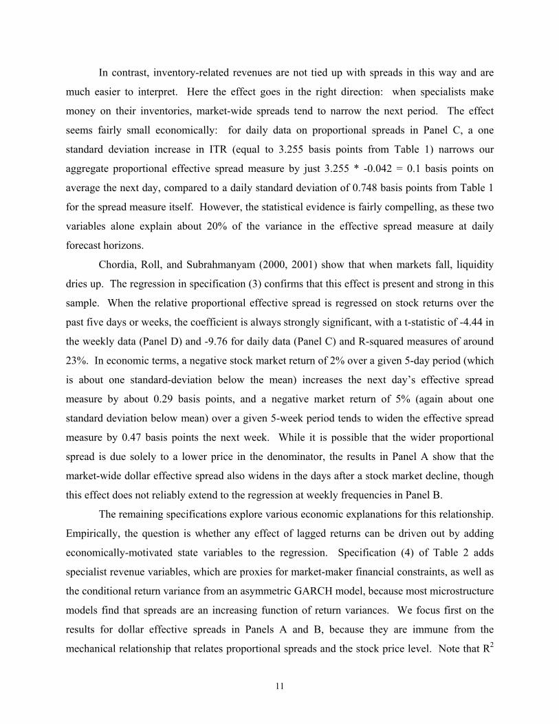
In contrast, inventory-related revenues are not tied up with spreads in this way and are
much easier to interpret. Here the effect goes in the right direction: when specialists make
money on their inventories, market-wide spreads tend to narrow the next period. The effect
seems fairly small economically: for daily data on proportional spreads in Panel C, a one
standard deviation increase in ITR (equal to 3.255 basis points from Table 1) narrows our
aggregate proportional effective spread measure by just 3.255 * -0.042 = 0.1 basis points on
average the next day, compared to a daily standard deviation of 0.748 basis points from Table 1
for the spread measure itself. However, the statistical evidence is fairly compelling, as these two
variables alone explain about 20% of the variance in the effective spread measure at daily
forecast horizons.
Chordia, Roll, and Subrahmanyam (2000, 2001) show that when markets fall, liquidity
dries up. The regression in specification (3) confirms that this effect is present and strong in this
sample. When the relative proportional effective spread is regressed on stock returns over the
past five days or weeks, the coefficient is always strongly significant, with a t-statistic of -4.44 in
the weekly data (Panel D) and -9.76 for daily data (Panel C) and R-squared measures of around
23%. In economic terms, a negative stock market return of 2% over a given 5-day period (which
is about one standard-deviation below the mean) increases the next day’s effective spread
measure by about 0.29 basis points, and a negative market return of 5% (again about one
standard deviation below mean) over a given 5-week period tends to widen the effective spread
measure by 0.47 basis points the next week. While it is possible that the wider proportional
spread is due solely to a lower price in the denominator, the results in Panel A show that the
market-wide dollar effective spread also widens in the days after a stock market decline, though
this effect does not reliably extend to the regression at weekly frequencies in Panel B.
The remaining specifications explore various economic explanations for this relationship.
Empirically, the question is whether any effect of lagged returns can be driven out by adding
economically-motivated state variables to the regression. Specification (4) of Table 2 adds
specialist revenue variables, which are proxies for market-maker financial constraints, as well as
the conditional return variance from an asymmetric GARCH model, because most microstructure
models find that spreads are an increasing function of return variances. We focus first on the
results for dollar effective spreads in Panels A and B, because they are immune from the
mechanical relationship that relates proportional spreads and the stock price level. Note that R2
11
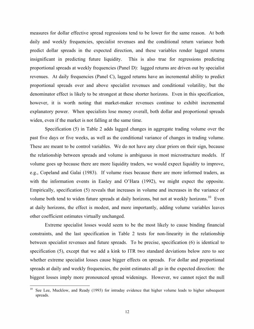
measures for dollar effective spread regressions tend to be lower for the same reason. At both
daily and weekly frequencies, specialist revenues and the conditional return variance both
predict dollar spreads in the expected direction, and these variables render lagged returns
insignificant in predicting future liquidity. This is also true for regressions predicting
proportional spreads at weekly frequencies (Panel D): lagged returns are driven out by specialist
revenues. At daily frequencies (Panel C), lagged returns have an incremental ability to predict
proportional spreads over and above specialist revenues and conditional volatility, but the
denominator effect is likely to be strongest at these shorter horizons. Even in this specification,
however, it is worth noting that market-maker revenues continue to exhibit incremental
explanatory power. When specialists lose money overall, both dollar and proportional spreads
widen, even if the market is not falling at the same time.
Specification (5) in Table 2 adds lagged changes in aggregate trading volume over the
past five days or five weeks, as well as the conditional variance of changes in trading volume.
These are meant to be control variables. We do not have any clear priors on their sign, because
the relationship between spreads and volume is ambiguous in most microstructure models. If
volume goes up because there are more liquidity traders, we would expect liquidity to improve,
e.g., Copeland and Galai (1983). If volume rises because there are more informed traders, as
with the information events in Easley and O’Hara (1992), we might expect the opposite.
Empirically, specification (5) reveals that increases in volume and increases in the variance of
volume both tend to widen future spreads at daily horizons, but not at weekly horizons.10 Even
at daily horizons, the effect is modest, and more importantly, adding volume variables leaves
other coefficient estimates virtually unchanged.
Extreme specialist losses would seem to be the most likely to cause binding financial
constraints, and the last specification in Table 2 tests for non-linearity in the relationship
between specialist revenues and future spreads. To be precise, specification (6) is identical to
specification (5), except that we add a kink to ITR two standard deviations below zero to see
whether extreme specialist losses cause bigger effects on spreads. For dollar and proportional
spreads at daily and weekly frequencies, the point estimates all go in the expected direction: the
biggest losses imply more pronounced spread widenings. However, we cannot reject the null 10 See Lee, Mucklow, and Ready (1993) for intraday evidence that higher volume leads to higher subsequent
spreads.
12

that there is no such kink, perhaps because the paucity of such large specialist losses implies
limited statistical power. We also obtain similar results when the kink is located at zero or one
standard deviation below zero.
For robustness, we have also estimated (but do not report) a number of other variants of
these specifications. The reported results are not driven by any particular subsample: the results
are present during each of the tick-size periods in our sample, and the results are present in
generally rising and generally falling markets. The results also hold for quoted spreads as well
as effective spreads.
4.1. A VAR as an alternative specification
Most of the variables in the regressions are calculated relative to recent means over the
interval [t – 10, t – 6]. This is a kind of hybrid approach, as it is somewhere between working
with levels and working with first differences. In this particular application, first differences are
not appropriate, since there is no theoretical reason to believe that any of the variables here
contain a unit root. Levels are not appropriate in the presence of apparent non-stationarity.
While we are not aware of any econometric theory that directly addresses our approach,
subtracting off recent means is a common approach in other areas of finance (cf. the relative T-
bill yield, introduced by Campbell (1991) and now very common in the return predictability
literature). The hybrid approach induces a modest amount of moving average behavior, which
requires the use of autocorrelation-consistent standard errors. To ensure that the main results are
not an artifact of this methodology, for robustness we use a somewhat more standard approach,
constructing a vector autoregression to capture the joint dynamics of spreads, returns, and
specialist revenues.
We estimate a daily VAR with 5 lags using detrended ITR, RTR, absolute market returns
(absret), market returns (retm), and effective spreads, either dollar (es) or proportional (espr).
Spreads are detrended using a piecewise linear trend within each tick size regime. Regime
means are subtracted for other variables. Granger causality results are based on bivariate VARs
with 5 lags and are reported in Table 3. The Granger causality results for the nonspread
variables are independent of whether spreads are in dollars or percentages and are, therefore,
reported only once. The results generally reflect the univariate correlations discussed earlier. It
is worth noting that ITR, absolute returns, and signed market returns all strongly Granger-cause
13
changes in effective spreads, but we cannot reject the null that RTR does not Granger-cause
innovations in spreads.
[ Insert Table 3 Here ]
The VAR allows us to examine impulse responses to orthogonalized shocks. The
ordering of the variables is ITR, RTR, absret, retm, followed by the effective spread. This
allows us to measure how a shock to ITR affects spreads in the future, and once this effect is
taken into account, we can determine whether market returns orthogonal to ITR have any
incremental ability to predict future spreads. The impulse response functions are displayed in
Figure 2 and reflect the response of either dollar or proportional effective spreads over the next
25 trading days to a unit standard deviation orthogonalized shock to one of the five variables.
Notice first that innovations to effective spreads are quite persistent, requiring a full month or so
to return to its detrended mean.
[ Insert Figure 2 Here ]
More interesting are the responses to shocks in the other variables. Shocks to ITR have
strong and persistent effects on spreads. A one-standard deviation negative shock to ITR causes
dollar spreads to widen by about 0.08 cents (0.2 basis points for proportional spreads). This is
the biggest effect on spreads of any of the five variables. A volatility shock in the form of a
large absolute return also causes spreads to widen, but its effect is smaller and less persistent. A
negative market return does not affect dollar spreads, but proportional spreads are modestly
affected for at least one month. The VARs provide a dynamic element that is not present in the
regressions, but the results on predicting spreads are virtually identical.
Overall, the aggregate evidence strongly supports a role for financial constraints in shaping
stock market liquidity. However, financial constraints should operate at the level of the financial
intermediary rather than at the aggregate level, so we turn next to more disaggregated evidence
to see if it too supports a capital constraint story.
14

5. Specialist firm revenues and liquidity in stocks assigned to the firm
If specialists are marginal liquidity suppliers, then a stock’s liquidity should suffer if its
specialist firm faces financing constraints. If financing constraints bind for all specialist firms at
the same time, then we should indeed see all the effects at the aggregate level. However, if
specialist firm revenues are imperfectly correlated, different specialist firms may face financing
constraints at different times, and we should be able to find empirical support for the constraints
hypothesis by identifying a relationship between specialist firm revenues and liquidity in that
firm’s assigned stocks, after controlling for aggregate effects.
At the end of our sample, there are only seven specialist firms, each with a broadly
diversified list of assigned stocks. Facing little idiosyncratic risk, specialist firms are likely to
earn revenues that are highly correlated with each other and with aggregate specialist revenues.
However, early in the sample, there are more than 40 specialist firms, resulting in considerable
cross-sectional dispersion in revenues and aiding identification.
To proceed, we disaggregate to the specialist firm level and create a panel with one
observation for each specialist firm for each day or week. We calculate aggregate gross trading
revenues each period for each specialist firm (gtrf), which is decomposed into overnight
inventory-related revenues (itrf) and intraday round-trip revenues (rtrf). A value-weighted
effective spread measure is calculated each day or week for all the stocks assigned to a given
specialist firm. We also calculate value-weighted returns (retp) on this portfolio of assigned
stocks in excess of the aggregate market return, along with the associated conditional volatility
(vretp) using an asymmetric GARCH model. We difference and demean these variables as in the
aggregate analysis of Section 3. Pooled regressions are estimated, and Rogers standard errors
are calculated which are robust to cross-sectional correlation.
[ Insert Table 4 Here ]
The results are in Table 4. Panels A and B analyze dollar effective spreads, at daily and
weekly frequencies respectively. Panels C and D display results for proportional effective
spreads. Specification (1) shows that, in contrast to earlier regressions at the aggregate level,
specialist firm gross trading revenues are significant predictors of next day liquidity in that
firm’s assigned stocks. As discussed earlier, there could be confounding effects between
15
intraday revenues (RTR) and future spreads, so we again decompose the specialist firm’s daily
revenues and focus on revenues that arise from overnight inventory (ITR). These effects in
specification (2) are quite strong, with t-statistics ranging from 7.7 to 11.8 depending on the
frequency and the spread measure.
We provide other intermediate specifications, but most relevant is specification (5),
which predicts next-period effective spreads on the value-weighted portfolio of assigned stocks
using specialist firm-level ITR and RTR, aggregate market returns and returns on the portfolio of
assigned stocks, and conditional volatility on the assigned stocks. Specialist firm trading
revenues always predict effective spreads, regardless of the frequency or spread measure. For
the dollar spread measure, the firm-level trading revenues drive out returns on the firm’s stocks.
This is not true for proportional spreads, but as we argued earlier, the presence of price in the
denominator can mechanically cause returns to predict proportional spreads.
In specification (6), we add a kink to specialist-firm ITR located at two within-specialist
standard deviations below zero. Compared to the similar exercise in Table 2, we find more
statistical evidence that the biggest specialist-firm losses cause more pronounced spread
widenings. In two of the four panels, there is reliable evidence of a kink, consistent with
financial constraints binding more severely following relatively large losses.
Overall, we conclude that at the specialist firm level, there is strong evidence that firm
trading revenues, but not returns on the portfolio of stocks assigned to the specialist firm, affect
next period’s spreads. This strongly supports the hypothesis that intermediary-level financial
performance affects liquidity.
6. Individual Stock Liquidity and Revenues
If time-variation in liquidity reflects financing constraints faced by intermediaries, the
relationship should operate at the intermediary firm level. Assuming that internal capital
markets are working correctly within the specialist firm and that the specialist firm is the main
liquidity provider, there should be no relationship between individual stock liquidity and
specialist revenues in that stock after controlling for effects at the specialist firm level.
To investigate this, we use a full panel of specialist revenue and individual-stock liquidity.
Pooled regressions are estimated for a panel of all NYSE stocks during the 1994-2004 sample
period. The dependent variable is the proportional effective spread during day or week t in stock
16

i relative to its average value during the interval [t–10, t–6], measured in basis points. This acts
something like a fixed effect, in that the explanatory variables do not have to explain across-
stock variation in average spread levels. Explanatory variables appear in pairs, with a stock-
specific and specialist firm version of each. There are specialist firm and stock-specific
inventory revenues (itrf and itrs), round-trip intraday revenues (rtrf and rtrs), and lagged stock
returns (retf and rets), where the own-stock return rets is the excess return over retf, which is the
value-weighted return on the portfolio of stocks assigned to the specialist firm. There are also
market-wide and stock-specific conditional return variances (vretm and vrets). As before,
revenues and returns are measured during the interval [t–5, t–1], and each variance is the time t–
1 forecast of the time t conditional return variance from a univariate asymmetric GARCH model,
measured relative to the conditional variance during the interval [t–10, t–6]. We continue to use
Rogers standard errors to control for contemporaneous correlation in error terms (Peterson
(2006)).
[ Insert Table 5 Here ]
We focus on specification (4) of Table 5, because it includes the specialist-firm level
variables that were found to explain time-variation in aggregated liquidity in the previous
section. Not surprisingly, those variables also affect individual-stock liquidity. In addition,
there is an extremely strong statistical relationship between lagged own-stock returns and future
individual-stock liquidity, with t-statistics that are over 60 for both the daily horizons in Panel A
and the weekly horizons in Panel B. At daily horizons, ITR at the individual stock level adds no
marginal explanatory power. The aggregate inventory revenue variable itrf still matters, but the
individual stock revenue variables are no longer significant in the daily data. In the weekly data,
the coefficient on firm-specific inventory revenue itrs is positive. This is good news for our
story. If the operative mechanism is intermediary financial constraints, this mechanism should
apply at the specialist-firm level, but not at the individual stock level.
Of course, this leaves unanswered the question of why own lagged returns affect own stock
liquidity so strongly. Part of the explanation is the denominator effect from using proportional
effective spreads. But the effect is still present when we use dollar effective spreads (results not
reported). Perhaps the information environment has changed, with market-makers worrying
17
more about adverse selection following a price decline. This hypothesis is worthy of future
study but would take us far afield from systematic time-variation in liquidity, the main object of
study here.
In sum, the individual stock analysis confirms that short-term changes in liquidity are driven
by more aggregated specialist firm revenues, not idiosyncratic individual stock revenues. This
finding maps directly into the capital constraints story, so, in some ways, our main task is
complete at this point. However, if we want a complete understanding of the interrelationships
between liquidity and specialist revenue, we need to understand as thoroughly as possible what
causes specialists to lose money, and that is the topic of the next two sections.
7. The Determinants of the Mean and Volatility of Specialist Revenues
Understanding market maker revenues involves examining these revenues in both the cross
section and time series. Given that the capital constraints story is primarily focused on the time-
series relationship between market maker revenues and liquidity, we begin our study of revenues
in the time series. To investigate this, we run time series regressions using daily or weekly
observations. The first set of regressions focuses on the first moment of market-maker revenues.
The dependent variable is specialist gross trading revenues (GTR) or one of its two components:
inventory-related trading revenues (ITR) or round-trip intraday trading revenues (RTR), each
measured at time t. Explanatory variables include first and second moments of returns and
trading volume, with each variable measured using information available at time t – 1. To be
more precise, right-hand side variables consist of log value-weighted market returns in percent
(ret), and log changes in aggregate trading volume (vol), each measured over the time interval [t
– 5, t – 1], the time t – 1 forecast of the time t return variance from an asymmetric GARCH
model (vret) and the unexpected realized return variance at time t (uvret), along with analogous
variables for the variance of volume changes (vvol and uvvol). As before, specialist revenues are
measured relative to the mean of the relevant tick-size regime, and conditional variances are
measured as changes from their average values during the interval [t – 10, t – 6]. Inference is
conducted using Newey-West standard errors with 10 lags.
Table 6 Panel A has the results for daily observations; results for weekly observations are in
Panel B. Specialist revenues, and especially intraday round-trip revenues RTR, tend to be higher
if volume has risen over the past five periods. Volume is quite persistent, so higher volume in
18
the recent past means higher volume today on average, on which the specialist tends to earn
more revenue.
[ Insert Table 6 Here ]
The most robust results are for the variance of returns. When conditional variance is high,
overall specialist revenue is high, and this result is driven by RTR, which itself reflects net
spread revenues realized by the specialist over the course of the trading day. It is not surprising
that spreads should be positively correlated with the conditional variance of returns; this is a
feature of virtually every microstructure model. But RTR represents spreads net of losses to
informed traders, and these are increasing in the conditional variance of returns. This result
would not arise in a microstructure model with perfectly competitive intermediaries. Specialist
market power could increase in more volatile markets, perhaps because communication lags are
relatively more important in fast markets, giving the specialist a greater last mover advantage.
Alternatively, this result could arise if intermediaries are risk averse or face financial constraints
that lead to risk averse behavior.
To try to separate these two explanations, we examine the riskiness of the specialist revenue
stream. The time-series regressions are virtually identical except for the dependent variable,
which now is the standard deviation of daily aggregate specialist revenues during week t, or the
standard deviation of daily ITR or RTR. The results are in Table 7, and they indicate strongly
that specialist revenue volatility is increasing in the conditional variance of returns. In fact, ITR
volatility and RTR volatility are both higher when return variance goes up. Thus, there is
support for the hypothesis that at least some of the additional specialist revenue in volatile
markets represents compensation for additional risk.
[ Insert Table 7 Here ]
8. The Cross Section of the Mean and Volatility of Revenues and Revenue Margins
Our last inquiry focuses on the variation in specialist revenues across stocks, in order to
determine where specialists (and potentially other intermediaries as well) face the biggest risks
19
and the biggest rewards. There has been some discussion in the literature about whether the
specialist revenue from trading the most active stocks helps to subsidize market-making in less
active stocks (Cao, Choe, and Hatheway (1997) and Huang and Liu (2003)). Our data can shed
light on this particular question. The cross-sectional distribution of specialist revenue is also
potentially important in understanding market-maker financial constraints. For instance, if only
a few stocks account for the vast majority of specialist revenues, then specialist losses in these
pivotal stocks may exert strong cross-effects on the liquidity of other stocks.
Our empirical analysis attempts to account for both the first and second moment of specialist
revenues, measured in dollars and as a fraction of specialist trading volume in that stock (which
we sometimes call the specialist’s operating margin). A Fama-MacBeth approach is used:
cross-sectional regressions are estimated for each month t, and we report the time-series average
of the resulting coefficients and conduct inference assuming independence across months. Stock
characteristics from the previous month include the log market cap (size), average daily turnover
(turn), the inverse of the month-end share price (invprc), the log return during the month in
percent (rets), the average daily log changes in dollar volume during the month (vols), and the
end-of-month t–1 forecast of the individual stock return variance on the first day of month t
using an asymmetric GARCH model (vrets), along with an analogous variable related to the
variance of volume changes (vvols) using a symmetric GARCH model. Conditional variances
are measured as changes from their average values during the interval [t–10, t–6].
The results are in Table 8. Specialists generate more trading revenue in large stocks, active
stocks, low-priced stocks, volatile stocks, and stocks with more variable trading volume. Most
of these results are quite intuitive. For example, more trading means more revenue, a faster
market (more volatility) gives the specialist a bigger advantage over other participants, and a low
share price means the minimum tick is more likely to bind, with larger profits to liquidity
providers.
[ Insert Table 8 Here ]
In contrast to specialist revenues, when we look at specialist margins, defined here as
specialist trading revenue per dollar of specialist trading volume, it is striking that none of these
20
cross-sectional regularities are reliably present. In fact, we cannot reject the hypothesis that
specialist margins are on average constant across stocks. This is a striking result, because the
null hypothesis, if true, means that specialists do not earn negative revenues on average on any
particular subset of stocks. Cross-subsidization may still be taking place, but these results
indicate that specialist firms are, at most, using revenues from active stocks to subsidize the
fixed costs of making a market in less active stocks. Put another way, if there are no fixed costs
then we find no evidence of cross-subsidization. To the extent that technology lowers these fixed
costs, e.g., through algorithmic liquidity supply, then the arguments for encouraging cross-
subsidization at the NYSE appear weak.
Even though specialist margins do not differ much across stocks, margin risk does vary
considerably. For example, specialist margins are more volatile in small stocks, high-priced
stocks, and stocks where trading volume is more variable. These results are also fairly intuitive.
For instance, information asymmetries are generally more severe in small-cap stocks, and
spreads tend to be wider. Specialists earn bigger spreads in these stocks but may ultimately lose
them if the counterparty turns out to be informed. In low-priced stocks, the minimum tick
enforces a minimum spread and thus a fairly certain stream of revenues.
In fact, these kinds of revenue and revenue volatility results may be most valuable because
they provide some insight into the risk management considerations at market-making firms.
Regressions like these are probably being used by risk managers at specialist firms, who may in
turn influence the cross-sectional allocation of specialist capital, perhaps thereby affecting the
cross-section and time-series of liquidity. The influence of revenue volatility thus seems like it
is worthy of additional study in future work.
9. Conclusion
In this paper, we use an 11-year panel of daily specialist revenues on individual NYSE stocks
to explore the relationship between market-maker revenue and liquidity. At the aggregate level
and at the specialist firm level, it turns out that when specialists lose money on their inventories,
effective spreads are significantly wider in the days or weeks that follow. When we run a horse
race between inventory-related specialist revenues, market returns, and conditional return
volatility at the aggregate market level, we find that both revenues and volatility have
21
incremental predictive power for future liquidity, and in most specifications market returns no
longer have incremental predictive power. This suggests that market-maker financial constraints
can help us understand time-variation in liquidity, while also acknowledging the traditional
mechanisms of microstructure theory that link price volatility and liquidity.
When we look at individual stocks, we find that at short horizons specialist revenues in
individual stocks do not have any marginal explanatory power for future changes in that stock’s
liquidity. Only aggregate specialist revenues or specialist firm revenues can predict future
liquidity, which is precisely what we would expect of a financial constraints model with broadly
diversified intermediaries.
We also investigate the variation in the level and risk of specialist revenues, both over time
and across stocks. The main time-series result is that aggregate specialist revenues are
increasing in conditional volatility. This effect is driven by intraday round-trip trades,
suggesting that the specialist’s structural advantage is more valuable in volatile markets. But
this higher average reward comes with higher risk, as aggregate revenue volatility is also greater
in volatile markets. Specialist revenues are highest for large stocks, active stocks, low-priced
stocks, volatile stocks, and stocks with more variable trading volume. However, the main cross-
sectional result is that specialist margins (specialist revenue per dollar of trading volume) are
essentially constant across stocks, implying that if there are no fixed costs then there is no cross-
subsidization.
But puzzles do remain. The most puzzling result is at the specialist firm level, where
specialist firm revenues do not drive out the relationship between spreads and lagged market
returns. It could be that there are other broadly diversified firms or funds who are also marginal
liquidity providers, in which case liquidity is affected not just by the specialist firm’s revenues
but also by broader market-wide state variables. Unfortunately, we do not have direct evidence
to bring to bear on this issue.
It is also interesting to note the strong relationship between individual stock liquidity and
lagged individual stock returns. This does not bear directly on the financial constraints
hypothesis, but the effect is so strong that it warrants future work. We suspect that the
information environment changes, with liquidity providers suffering greater losses to informed
traders following a share price decline, and we are currently gathering price impact data to assess
this explanation.
22
Ultimately, our revenue measures are noisy instruments for the bite of financial constraints.
Even more useful would be direct evidence on changes in collateral requirements, credit limits,
or financing costs imposed by lenders in response to shocks. Unfortunately, these are not readily
available to us. However, we are currently looking at specialist consolidation in the late 1990’s.
In 1994, at the beginning of our sample period, there were 41 specialist firms. In 2004, at the
end of our sample period, there were only 7. Many of these mergers were undertaken explicitly
to shore up market maker capital. If small specialist firms faced fairly onerous constraints just
prior to being taken over, such mergers could be useful instruments for an even better
identification of financing constraints.
23

References Amihud, Yakov, and Haim Mendelson, 1980, Dealership market: Market making with inventory, Journal of Financial Economics 8, 31–53. Amihud, Yakov, Haim Mendelson, and Lasse Pedersen, 2005, Liquidity and asset prices, Foundations and Trends in Finance 1, 269-364. Attari, Mukarram, Antonio Mello, and Martin Ruckes, 2005, Arbitraging arbitrageurs, Journal of Finance 60, 2471-2511. Bessembinder, Hendrik, 2003, Issues in assessing trade execution costs, Journal of Financial Markets 6, 233-257. Boehmer, Ekkehart and Julie Wu, 2006, Order flow and prices, working paper. Brunnermeier, Markus, and Lasse Pedersen, 2005, Predatory trading, Journal of Finance 60, 1825-1863. Brunnermeier, Markus, and Lasse Pedersen, 2006, Market liquidity and funding liquidity, working paper. Campbell, John, 1991, A variance decomposition for stock returns, Economic Journal 101, 157-179. Cao, Charles, Hyuk Choe, and Frank Hatheway, 1997, Does the specialist matter? Differential execution costs and intersecurity subsidization on the New York Stock Exchange, Journal of Finance 52, 1615-1640. Chordia, Tarun, Richard Roll, and Avanidhar Subrahmanyam, 2000, Commonality in liquidity, Journal of Financial Economics 56, 3-28. Chordia, Tarun, Richard Roll, and Avanidhar Subrahmanyam, 2001, Market liquidity and trading activity, Journal of Finance 56, 501-530. Chordia, Tarun, Asani Sarkar, and Avanidhar Subrahmanyam, 2005, An Empirical Analysis of Stock and Bond Market Liquidity, Review of Financial Studies 18, 85-129. Copeland, Tom, and Dan Galai, 1983, Information effects on the bid/ask spread, Journal of Finance 38, 1457-1469. Coughenour, Jay, and Mohsen Saad, 2004, Common market makers and commonality in liquidity, Journal of Financial Economics 73, 37-69. Coughenour, Jay, and Lawrence Harris, 2004, Specialist profits and the minimum price increment. working paper.
24

Easley, David, and Maureen O’Hara, 1992,Time and the process of security price adjustment, Journal of Finance 47, 577-605. Glosten, Lawrence, 1989, Insider trading, liquidity, and the role of the monopolist specialist, Journal of Business 48, 211–235. Glosten, Lawrence, Ravi Jaganathan, and David Runkle, 1993, On the relation between the expected value and the volatility of the nominal excess return on stocks, Journal of Finance 48, 1779–1801. Glosten, Lawrence, and Paul Milgrom, 1985, Bid, ask and transaction prices in a specialist market with heterogeneously informed traders, Journal of Financial Economics 14, 71–100. Grossman, Sanford, and Merton Miller, 1988, Liquidity and market structure, Journal of Finance 43, 617–633. Gromb, Denis, and Dimitri Vayanos, 2002, Equilibrium and welfare in markets with financially constrained arbitrageurs, Journal of Financial Economics 66, 361-407. Hameed, Allaudeen, Wenjin Kang, and S. Viswanathan, 2006, Stock market decline and liquidity, working paper. Hansch, Oliver, Nayaran Naik, and S. Viswanathan, 1999, Best execution, internalization, preferencing and dealer profits , Journal of Finance 54, 1799-1828. Hasbrouck, Joel, and Duane Seppi, 2001, Common factors in prices, order flows and liquidity, Journal of Financial Economics 59, 383-411. Hasbrouck, Joel, and George Sofianos, 1993, The trades of market-makers: An analysis of NYSE specialists, Journal of Finance 48, 1565-1594. Hendershott, Terrence, Pamela Moulton, and Mark Seasholes, 2007, Market maker inventories and stock market liquidity, working paper. Hendershott, Terrence, and Mark Seasholes, 2007, Market maker inventories and stock prices, American Economic Review 97, 210-214.. Ho, Thomas, and Hans Stoll, 1981, Optimal dealer pricing under transactions and return uncertainty, Journal of Financial Economics 9, 47-73. Ho, Thomas, and Hans Stoll, 1983, The dynamics of dealer markets under competition, Journal of Finance 38, 1053–1074. Huang, Roger, and Jerry Liu, 2003, Do individual NYSE specialists subsidize illiquid stocks? working paper.
25

Ip, Greg, and Susanne Craig, 2003, Trading cases: NYSE's `Specialist' probe puts precious asset at risk, Wall Street Journal, April 18, 2003, A1. Jones, Charles, 2006, A century of stock market liquidity and trading costs, working paper. Kyle, Albert, 1985, Continuous auctions and insider trading, Econometrica 53, 1315-1336. Kyle, Albert, and Wei Xiong, 2001, Contagion as a wealth effect, Journal of Finance 56, 1401-1440. Lee, Charles, Belinda Mucklow, and Mark Ready, 1993, Spreads, depths, and the impact of earnings information: An intraday analysis, Review of Financial Studies 6, 345-374. Lee, Charles, and Mark Ready, 1991, Inferring trade direction from intraday data, Journal of Finance 46, 733-747. Naik, Narayan, and Pradeep Yadav, 2003, Risk management with derivative by dealers and market quality in government bond markets, Journal of Finance 58, 1873-1904. Panayides, Marios, 2006, Affirmative obligations and market making with inventory, Journal Of Financial Economics, forthcoming. Petersen, Mitchell, 2006, Estimating standard errors in finance panel data sets: Comparing approaches, Kellogg Finance Dept. Working Paper No. 329, Available at SSRN: http://ssrn.com/abstract=661481. Sofianos, George, 1995, Specialist Gross Trading Revenues at the New York Stock Exchange, working paper. Stoll, Hans, 1978, The supply of dealer services in security markets, Journal of Finance 33, 1133-1151. Weill, Pierre-Olivier, 2006, Leaning against the wind, working paper. White, Halbert, 1980, A heteroscedasticity-consistent covariance matrix estimator and a direct test of heteroskedasticity, Econometrica 48, 817-838. Yuan, Kathy, 2005, Asymmetric price movements and borrowing constraints: A rational expectations equilibrium model of crises, contagion, and confusion, Journal of Finance 60, 379-411.
26
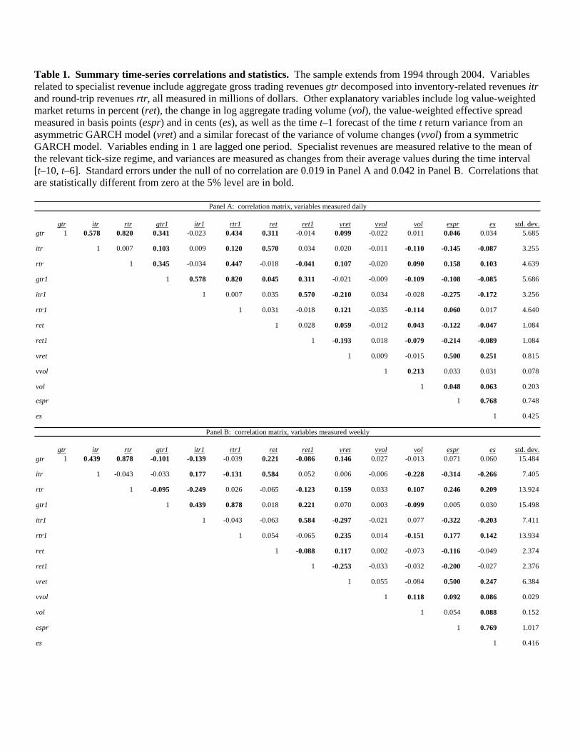
Table 1. Summary time-series correlations and statistics. The sample extends from 1994 through 2004. Variables related to specialist revenue include aggregate gross trading revenues gtr decomposed into inventory-related revenues itr and round-trip revenues rtr, all measured in millions of dollars. Other explanatory variables include log value-weighted market returns in percent (ret), the change in log aggregate trading volume (vol), the value-weighted effective spread measured in basis points (espr) and in cents (es), as well as the time t–1 forecast of the time t return variance from an asymmetric GARCH model (vret) and a similar forecast of the variance of volume changes (vvol) from a symmetric GARCH model. Variables ending in 1 are lagged one period. Specialist revenues are measured relative to the mean of the relevant tick-size regime, and variances are measured as changes from their average values during the time interval [t–10, t–6]. Standard errors under the null of no correlation are 0.019 in Panel A and 0.042 in Panel B. Correlations that are statistically different from zero at the 5% level are in bold.
gtr itr rtr gtr1 itr1 rtr1 ret ret1 vret vvol vol espr es std. dev.gtr 1 0.578 0.820 0.341 -0.023 0.434 0.311 -0.014 0.099 -0.022 0.011 0.046 0.034 5.685
itr 1 0.007 0.103 0.009 0.120 0.570 0.034 0.020 -0.011 -0.110 -0.145 -0.087 3.255
rtr 1 0.345 -0.034 0.447 -0.018 -0.041 0.107 -0.020 0.090 0.158 0.103 4.639
gtr1 1 0.578 0.820 0.045 0.311 -0.021 -0.009 -0.109 -0.108 -0.085 5.686
itr1 1 0.007 0.035 0.570 -0.210 0.034 -0.028 -0.275 -0.172 3.256
rtr1 1 0.031 -0.018 0.121 -0.035 -0.114 0.060 0.017 4.640
ret 1 0.028 0.059 -0.012 0.043 -0.122 -0.047 1.084
ret1 1 -0.193 0.018 -0.079 -0.214 -0.089 1.084
vret 1 0.009 -0.015 0.500 0.251 0.815
vvol 1 0.213 0.033 0.031 0.078
vol 1 0.048 0.063 0.203
espr 1 0.768 0.748
es 1 0.425
gtr itr rtr gtr1 itr1 rtr1 ret ret1 vret vvol vol espr es std. dev.gtr 1 0.439 0.878 -0.101 -0.139 -0.039 0.221 -0.086 0.146 0.027 -0.013 0.071 0.060 15.484
itr 1 -0.043 -0.033 0.177 -0.131 0.584 0.052 0.006 -0.006 -0.228 -0.314 -0.266 7.405
rtr 1 -0.095 -0.249 0.026 -0.065 -0.123 0.159 0.033 0.107 0.246 0.209 13.924
gtr1 1 0.439 0.878 0.018 0.221 0.070 0.003 -0.099 0.005 0.030 15.498
itr1 1 -0.043 -0.063 0.584 -0.297 -0.021 0.077 -0.322 -0.203 7.411
rtr1 1 0.054 -0.065 0.235 0.014 -0.151 0.177 0.142 13.934
ret 1 -0.088 0.117 0.002 -0.073 -0.116 -0.049 2.374
ret1 1 -0.253 -0.033 -0.032 -0.200 -0.027 2.376
vret 1 0.055 -0.084 0.500 0.247 6.384
vvol 1 0.118 0.092 0.086 0.029
vol 1 0.054 0.088 0.152
espr 1 0.769 1.017
es 1 0.416
Panel A: correlation matrix, variables measured daily
Panel B: correlation matrix, variables measured weekly
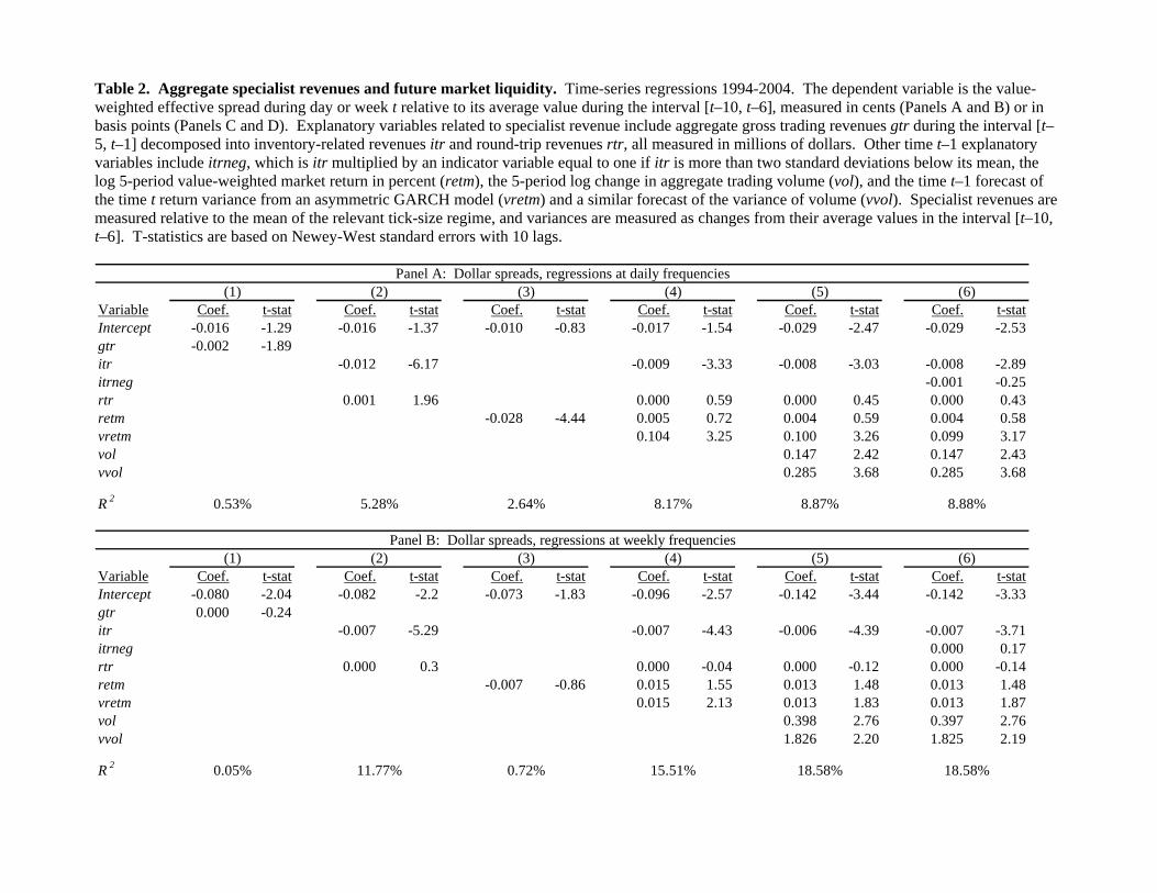
Table 2. Aggregate specialist revenues and future market liquidity. Time-series regressions 1994-2004. The dependent variable is the value-weighted effective spread during day or week t relative to its average value during the interval [t–10, t–6], measured in cents (Panels A and B) or in basis points (Panels C and D). Explanatory variables related to specialist revenue include aggregate gross trading revenues gtr during the interval [t–5, t–1] decomposed into inventory-related revenues itr and round-trip revenues rtr, all measured in millions of dollars. Other time t–1 explanatory variables include itrneg, which is itr multiplied by an indicator variable equal to one if itr is more than two standard deviations below its mean, the log 5-period value-weighted market return in percent (retm), the 5-period log change in aggregate trading volume (vol), and the time t–1 forecast of the time t return variance from an asymmetric GARCH model (vretm) and a similar forecast of the variance of volume (vvol). Specialist revenues are measured relative to the mean of the relevant tick-size regime, and variances are measured as changes from their average values in the interval [t–10, t–6]. T-statistics are based on Newey-West standard errors with 10 lags.
Variable Coef. t-stat Coef. t-stat Coef. t-stat Coef. t-stat Coef. t-stat Coef. t-statIntercept -0.016 -1.29 -0.016 -1.37 -0.010 -0.83 -0.017 -1.54 -0.029 -2.47 -0.029 -2.53gtr -0.002 -1.89itr -0.012 -6.17 -0.009 -3.33 -0.008 -3.03 -0.008 -2.89itrneg -0.001 -0.25rtr 0.001 1.96 0.000 0.59 0.000 0.45 0.000 0.43retm -0.028 -4.44 0.005 0.72 0.004 0.59 0.004 0.58vretm 0.104 3.25 0.100 3.26 0.099 3.17vol 0.147 2.42 0.147 2.43vvol 0.285 3.68 0.285 3.68
R 2
Variable Coef. t-stat Coef. t-stat Coef. t-stat Coef. t-stat Coef. t-stat Coef. t-statIntercept -0.080 -2.04 -0.082 -2.2 -0.073 -1.83 -0.096 -2.57 -0.142 -3.44 -0.142 -3.33gtr 0.000 -0.24itr -0.007 -5.29 -0.007 -4.43 -0.006 -4.39 -0.007 -3.71itrneg 0.000 0.17rtr 0.000 0.3 0.000 -0.04 0.000 -0.12 0.000 -0.14retm -0.007 -0.86 0.015 1.55 0.013 1.48 0.013 1.48vretm 0.015 2.13 0.013 1.83 0.013 1.87vol 0.398 2.76 0.397 2.76vvol 1.826 2.20 1.825 2.19
R 2
(4) (5)
0.53%
(1) (2) (3)Panel A: Dollar spreads, regressions at daily frequencies
18.58%
8.87%
(1) (2)
0.05% 11.77% 0.72% 15.51%
(3) (6)
18.58%
Panel B: Dollar spreads, regressions at weekly frequencies
(6)
8.88%
(4) (5)
5.28% 2.64% 8.17%
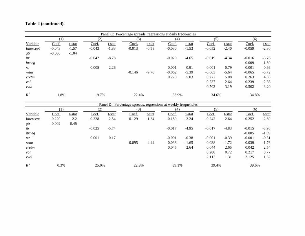
Table 2 (continued).
Variable Coef. t-stat Coef. t-stat Coef. t-stat Coef. t-stat Coef. t-stat Coef. t-statIntercept -0.043 -1.57 -0.043 -1.83 -0.013 -0.58 -0.030 -1.53 -0.052 -2.40 -0.059 -2.80gtr -0.006 -1.84itr -0.042 -8.78 -0.020 -4.65 -0.019 -4.34 -0.016 -3.76itrneg -0.009 -1.50rtr 0.005 2.26 0.001 0.91 0.001 0.79 0.001 0.66retm -0.146 -9.76 -0.062 -5.39 -0.063 -5.64 -0.065 -5.72vretm 0.278 5.03 0.272 5.08 0.263 4.83vol 0.237 2.64 0.239 2.66vvol 0.503 3.19 0.502 3.20
R 2
Variable Coef. t-stat Coef. t-stat Coef. t-stat Coef. t-stat Coef. t-stat Coef. t-statIntercept -0.220 -2.2 -0.228 -2.54 -0.129 -1.34 -0.189 -2.24 -0.242 -2.64 -0.252 -2.69gtr -0.002 -0.45itr -0.025 -5.74 -0.017 -4.95 -0.017 -4.83 -0.015 -3.98itrneg -0.005 -1.09rtr 0.001 0.17 -0.001 -0.38 -0.001 -0.39 -0.001 -0.31retm -0.095 -4.44 -0.038 -1.65 -0.038 -1.72 -0.039 -1.76vretm 0.045 2.64 0.044 2.65 0.042 2.54vol 0.200 0.72 0.217 0.77vvol 2.112 1.31 2.125 1.32
R 2
22.4% 33.9%
(5)Panel C: Percentage spreads, regressions at daily frequencies
(1) (2) (3) (4) (5)
34.6%1.8% 19.7%
(1) (2) (3) (4) (6)
34.8%
(6)
39.6%
Panel D: Percentage spreads, regressions at weekly frequencies
39.4%0.3% 25.0% 22.9% 39.1%
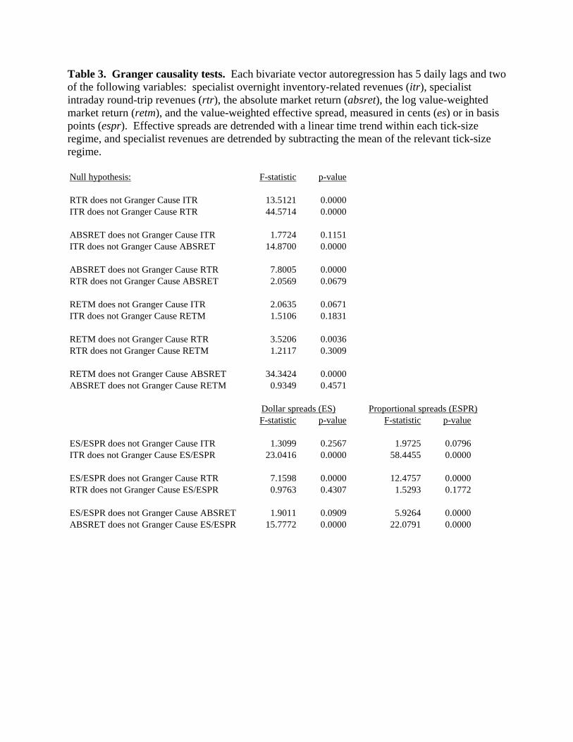
Table 3. Granger causality tests. Each bivariate vector autoregression has 5 daily lags and two of the following variables: specialist overnight inventory-related revenues (itr), specialist intraday round-trip revenues (rtr), the absolute market return (absret), the log value-weighted market return (retm), and the value-weighted effective spread, measured in cents (es) or in basis points (espr). Effective spreads are detrended with a linear time trend within each tick-size regime, and specialist revenues are detrended by subtracting the mean of the relevant tick-size regime. Null hypothesis: F-statistic p-value
RTR does not Granger Cause ITR 13.5121 0.0000ITR does not Granger Cause RTR 44.5714 0.0000
ABSRET does not Granger Cause ITR 1.7724 0.1151ITR does not Granger Cause ABSRET 14.8700 0.0000
ABSRET does not GrangeRTR does not Granger Cau
RETM does not Granger CITR does not Granger Cau
RETM does not Granger CRTR does not Granger Cau
RETM does not Granger CABSRET does not Grange
r Cause RTR 7.8005 0.0000se ABSRET 2.0569 0.0679
ause ITR 2.0635 0.0671se RETM 1.5106 0.1831
ause RTR 3.5206 0.0036se RETM 1.2117 0.3009
ause ABSRET 34.3424 0.0000r Cause RETM 0.9349 0.4571
F-statistic p-value F-statistic p-value
ES/ESPR does not GrangeITR does not Granger Cau
ES/ESPR does not GrangeRTR does not Granger Cau
ES/ESPR does not GrangeABSRET does not Grange
r Cause ITR 1.3099 0.2567 1.9725 0.0796se ES/ESPR 23.0416 0.0000 58.4455 0.0000
r Cause RTR 7.1598 0.0000 12.4757 0.0000se ES/ESPR 0.9763 0.4307 1.5293 0.1772
r Cause ABSRET 1.9011 0.0909 5.9264 0.0000r Cause ES/ESPR 15.7772 0.0000 22.0791 0.0000
Dollar spreads (ES) Proportional spreads (ESPR)
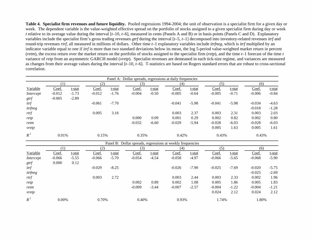
Table 4. Specialist firm revenues and future liquidity. Pooled regressions 1994-2004; the unit of observation is a specialist firm for a given day or week. The dependent variable is the value-weighted effective spread on the portfolio of stocks assigned to a given specialist firm during day or week t relative to its average value during the interval [t–10, t–6], measured in cents (Panels A and B) or in basis points (Panels C and D). Explanatory variables include the specialist firm’s gross trading revenues gtrf during the interval [t–5, t–1] decomposed into inventory-related revenues itrf and round-trip revenues rtrf, all measured in millions of dollars. Other time t–1 explanatory variables include itrfneg, which is itrf multiplied by an indicator variable equal to one if itrf is more than two standard deviations below its mean, the log 5-period value-weighted market return in percent (retm), the excess return over the market return on the portfolio of stocks assigned to the specialist firm (retp), and the time t–1 forecast of the time t variance of retp from an asymmetric GARCH model (vretp). Specialist revenues are demeaned in each tick-size regime, and variances are measured as changes from their average values during the interval [t–10, t–6]. T-statistics are based on Rogers standard errors that are robust to cross-sectional correlation.
Variable Coef. t-stat Coef. t-stat Coef. t-stat Coef. t-stat Coef. t-stat Coef. t-statIntercept -0.012 -1.73 -0.012 -1.76 -0.004 -0.50 -0.005 -0.64 -0.005 -0.71 -0.006 -0.84gtrf -0.005 -2.89itrf -0.061 -7.70 -0.041 -5.98 -0.041 -5.98 -0.034 -4.63itrfneg -0.018 -1.28rtrf 0.005 3.16 0.003 2.37 0.003 2.31 0.003 2.03retp 0.000 0.09 0.001 0.29 0.002 0.82 0.002 0.80retm -0.032 -6.60 -0.029 -5.94 -0.028 -6.03 -0.028 -6.03vretp 0.005 1.63 0.005 1.61
R 2
Variable Coef. t-stat Coef. t-stat Coef. t-stat Coef. t-stat Coef. t-stat Coef. t-statIntercept -0.066 -5.55 -0.066 -5.70 -0.054 -4.54 -0.058 -4.97 -0.066 -5.65 -0.068 -5.90gtrf 0.000 0.12itrf -0.029 -8.25 -0.026 -7.90 -0.025 -7.69 -0.020 -5.75itrfneg -0.025 -2.69rtrf 0.003 2.72 0.003 2.44 0.003 2.33 0.002 1.96retp 0.002 0.89 0.002 1.08 0.005 1.86 0.005 1.83retm -0.009 -3.44 -0.007 -2.57 -0.004 -1.22 -0.004 -1.21vretp 0.024 2.12 0.024 2.12
R 2
(3)
1.74%0.00% 0.70% 0.40% 0.93%
(5)Panel A: Dollar spreads, regressions at daily frequencies
(4) (5)
0.15% 0.35% 0.42% 0.43%
(1) (2)
(6)
0.43%
(6)
1.80%
Panel B: Dollar spreads, regressions at weekly frequencies
0.01%
(1) (2) (3) (4)
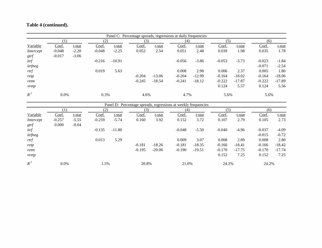
Table 4 (continued).
Variable Coef. t-stat Coef. t-stat Coef. t-stat Coef. t-stat Coef. t-stat Coef. t-statIntercept -0.048 -2.20 -0.048 -2.25 0.052 2.54 0.051 2.48 0.039 1.98 0.035 1.78gtrf -0.017 -3.06itrf -0.216 -10.91 -0.056 -3.86 -0.053 -3.73 -0.023 -1.84itrfneg -0.071 -2.54rtrf 0.019 5.63 0.008 2.98 0.006 2.37 0.005 1.80retp -0.204 -13.06 -0.204 -12.99 -0.164 -18.02 -0.164 -18.06retm -0.245 -18.54 -0.241 -18.12 -0.222 -17.87 -0.222 -17.89vretp 0.124 5.57 0.124 5.56
R 2
Variable Coef. t-stat Coef. t-stat Coef. t-stat Coef. t-stat Coef. t-stat Coef. t-statIntercept -0.257 -5.55 -0.259 -5.74 0.160 3.92 0.152 3.72 0.107 2.79 0.105 2.73gtrf 0.000 -0.04itrf -0.135 -11.80 -0.048 -5.50 -0.040 -4.96 -0.037 -4.09itrfneg -0.015 -0.72rtrf 0.013 5.29 0.009 3.07 0.008 2.89 0.008 2.80retp -0.181 -18.26 -0.181 -18.35 -0.166 -18.41 -0.166 -18.42retm -0.195 -20.06 -0.190 -19.51 -0.170 -17.75 -0.170 -17.74vretp 0.152 7.25 0.152 7.25
R 2
(6)
5.6%
(6)
0.0% 1.5% 20.8% 21.0% 24.2% 24.2%
Panel D: Percentage spreads, regressions at weekly frequencies
5.6%0.0% 0.3% 4.6% 4.7%
(1) (2) (3) (4) (5)
(1) (2) (3) (4) (5)Panel C: Percentage spreads, regressions at daily frequencies
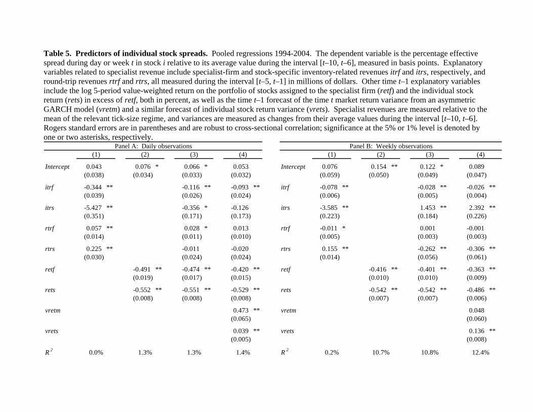
Table 5. Predictors of individual stock spreads. Pooled regressions 1994-2004. The dependent variable is the percentage effective spread during day or week t in stock i relative to its average value during the interval [t–10, t–6], measured in basis points. Explanatory variables related to specialist revenue include specialist-firm and stock-specific inventory-related revenues itrf and itrs, respectively, and round-trip revenues rtrf and rtrs, all measured during the interval [t–5, t–1] in millions of dollars. Other time t–1 explanatory variables include the log 5-period value-weighted return on the portfolio of stocks assigned to the specialist firm (retf) and the individual stock return (rets) in excess of retf, both in percent, as well as the time t–1 forecast of the time t market return variance from an asymmetric GARCH model (vretm) and a similar forecast of individual stock return variance (vrets). Specialist revenues are measured relative to the mean of the relevant tick-size regime, and variances are measured as changes from their average values during the interval [t–10, t–6]. Rogers standard errors are in parentheses and are robust to cross-sectional correlation; significance at the 5% or 1% level is denoted by one or two asterisks, respectively.
Intercept 0.043 0.076 * 0.066 * 0.053 Intercept 0.076 0.154 ** 0.122 * 0.089(0.038) (0.034) (0.033) (0.032) (0.059) (0.050) (0.049) (0.047)
itrf -0.344 ** -0.116 ** -0.093 ** itrf -0.078 ** -0.028 ** -0.026 **(0.039) (0.026) (0.024) (0.006) (0.005) (0.004)
itrs -5.427 ** -0.356 * -0.126 itrs -3.585 ** 1.453 ** 2.392 **(0.351) (0.171) (0.173) (0.223) (0.184) (0.226)
rtrf 0.057 ** 0.028 * 0.013 rtrf -0.011 * 0.001 -0.001(0.014) (0.011) (0.010) (0.005) (0.003) (0.003)
rtrs 0.225 ** -0.011 -0.020 rtrs 0.155 ** -0.262 ** -0.306 **(0.030) (0.024) (0.024) (0.014) (0.056) (0.061)
retf -0.491 ** -0.474 ** -0.420 ** retf -0.416 ** -0.401 ** -0.363 **(0.019) (0.017) (0.015) (0.010) (0.010) (0.009)
rets -0.552 ** -0.551 ** -0.529 ** rets -0.542 ** -0.542 ** -0.486 **(0.008) (0.008) (0.008) (0.007) (0.007) (0.006)
vretm 0.473 ** vretm 0.048(0.065) (0.060)
vrets 0.039 ** vrets 0.136 **(0.005) (0.008)
R 2 R 20.0% 1.3% 1.3% 1.4%
Panel A: Daily observations Panel B: Weekly observations(1) (2) (3) (4)(1) (2) (3) (4)
0.2% 10.7% 10.8% 12.4%
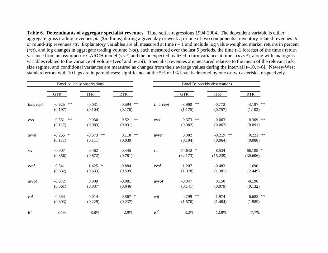
Table 6. Determinants of aggregate specialist revenues. Time-series regressions 1994-2004. The dependent variable is either aggregate gross trading revenues gtr ($millions) during a given day or week t, or one of two components: inventory-related revenues itr or round-trip revenues rtr. Explanatory variables are all measured at time t – 1 and include log value-weighted market returns in percent (ret), and log changes in aggregate trading volume (vol), each measured over the last 5 periods, the time t–1 forecast of the time t return variance from an asymmetric GARCH model (vret) and the unexpected realized return variance at time t (uvret), along with analogous variables related to the variance of volume (vvol and uvvol). Specialist revenues are measured relative to the mean of the relevant tick-size regime, and conditional variances are measured as changes from their average values during the interval [t–10, t–6]. Newey-West standard errors with 10 lags are in parentheses; significance at the 5% or 1% level is denoted by one or two asterisks, respectively.
GTR ITR RTR GTR ITR RTR
Intercept -0.625 ** -0.031 -0.594 ** Intercept -3.960 ** -0.772 -3.187 **(0.197) (0.104) (0.170) (1.175) (0.757) (1.103)
vret 0.551 ** 0.030 0.521 ** vret 0.373 ** 0.063 0.309 **(0.117) (0.083) (0.091) (0.082) (0.062) (0.091)
uvret -0.255 * -0.373 ** 0.118 ** uvret 0.002 -0.219 ** 0.221 **(0.111) (0.111) (0.039) (0.104) (0.064) (0.080)
ret -0.907 -0.462 -0.445 ret 74.642 * 8.534 66.108 *(0.856) (0.872) (0.781) (32.173) (15.239) (30.606)
vvol 0.541 1.425 * -0.884 vvol 1.207 -0.483 1.690(0.832) (0.633) (0.539) (1.978) (1.381) (2.449)
uvvol -0.072 0.009 -0.081 uvvol -0.047 0.150 -0.196(0.061) (0.037) (0.046) (0.141) (0.079) (0.132)
vol 0.554 -0.014 0.567 * vol 4.709 ** -1.974 6.683 **(0.303) (0.229) (0.237) (1.570) (1.484) (1.989)
R 2 3.1% 8.8% 2.9% R 2 3.2% 12.9% 7.7%
Panel A: daily observations Panel B: weekly observations
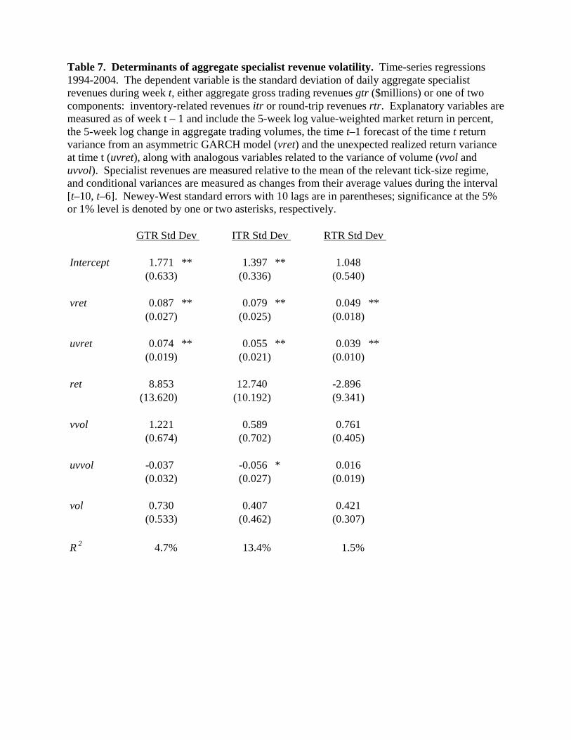
Table 7. Determinants of aggregate specialist revenue volatility. Time-series regressions 1994-2004. The dependent variable is the standard deviation of daily aggregate specialist revenues during week t, either aggregate gross trading revenues gtr ($millions) or one of two components: inventory-related revenues itr or round-trip revenues rtr. Explanatory variables are measured as of week t – 1 and include the 5-week log value-weighted market return in percent, the 5-week log change in aggregate trading volumes, the time t–1 forecast of the time t return variance from an asymmetric GARCH model (vret) and the unexpected realized return variance at time t (uvret), along with analogous variables related to the variance of volume (vvol and uvvol). Specialist revenues are measured relative to the mean of the relevant tick-size regime, and conditional variances are measured as changes from their average values during the interval [t–10, t–6]. Newey-West standard errors with 10 lags are in parentheses; significance at the 5% or 1% level is denoted by one or two asterisks, respectively.
Intercept 1.771 ** 1.397 ** 1.048(0.633) (0.336) (0.540)
vret 0.087 ** 0.079 ** 0.049 **(0.027) (0.025) (0.018)
uvret 0.074 ** 0.055 ** 0.039 **(0.019) (0.021) (0.010)
ret 8.853 12.740 -2.896(13.620) (10.192) (9.341)
vvol 1.221 0.589 0.761(0.674) (0.702) (0.405)
uvvol -0.037 -0.056 * 0.016(0.032) (0.027) (0.019)
vol 0.730 0.407 0.421(0.533) (0.462) (0.307)
R 2 4.7% 13.4% 1.5%
GTR Std Dev ITR Std Dev RTR Std Dev
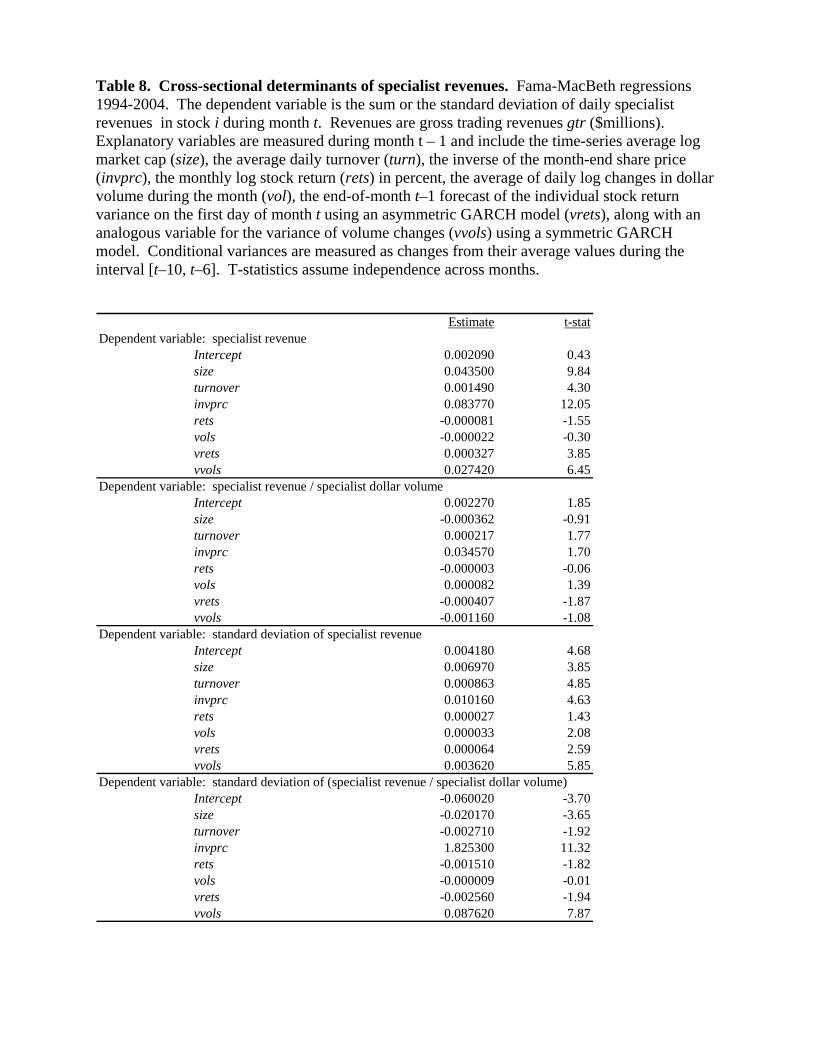
Table 8. Cross-sectional determinants of specialist revenues. Fama-MacBeth regressions 1994-2004. The dependent variable is the sum or the standard deviation of daily specialist revenues in stock i during month t. Revenues are gross trading revenues gtr ($millions). Explanatory variables are measured during month t – 1 and include the time-series average log market cap (size), the average daily turnover (turn), the inverse of the month-end share price (invprc), the monthly log stock return (rets) in percent, the average of daily log changes in dollar volume during the month (vol), the end-of-month t–1 forecast of the individual stock return variance on the first day of month t using an asymmetric GARCH model (vrets), along with an analogous variable for the variance of volume changes (vvols) using a symmetric GARCH model. Conditional variances are measured as changes from their average values during the interval [t–10, t–6]. T-statistics assume independence across months.
Estimate t-statDependent variable: specialist reven
Interceptsizeturnoverinvprcretsvolsvretsvvols
Dependent variable: specialist revenInterceptsizeturnoverinvprcretsvolsvretsvvols
Dependent variable: standard deviInterceptsizeturnoverinvprcretsvolsvretsvvols
Dependent variable: standard deviInterceptsizeturnoverinvprcretsvolsvretsvvols
ue0.002090 0.430.043500 9.840.001490 4.300.083770 12.05
-0.000081 -1.55-0.000022 -0.300.000327 3.850.027420 6.45
ue / specialist dollar volume0.002270 1.85
-0.000362 -0.910.000217 1.770.034570 1.70
-0.000003 -0.060.000082 1.39
-0.000407 -1.87-0.001160 -1.08
ation of specialist revenue0.004180 4.680.006970 3.850.000863 4.850.010160 4.630.000027 1.430.000033 2.080.000064 2.590.003620 5.85
ation of (specialist revenue / specialist dollar volume)-0.060020 -3.70-0.020170 -3.65-0.002710 -1.921.825300 11.32
-0.001510 -1.82-0.000009 -0.01-0.002560 -1.940.087620 7.87
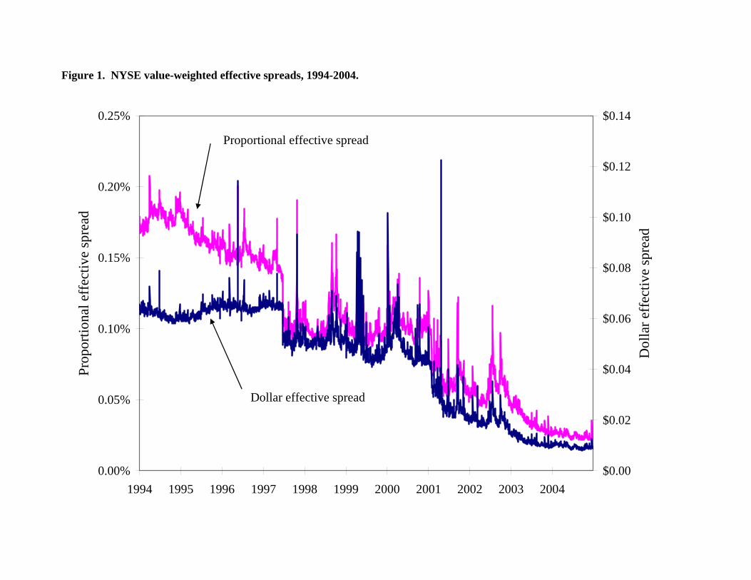
Figure 1. NYSE value-weighted effective spreads, 1994-2004.
0.00%
0.05%
0.10%
0.15%
0.20%
0.25%
1994 1995 1996 1997 1998 1999 2000 2001 2002 2003 2004
Prop
ortio
nal e
ffec
tive
spre
ad
$0.00
$0.02
$0.04
$0.06
$0.08
$0.10
$0.12
$0.14
Dol
lar e
ffec
tive
spre
ad
Dollar effective spread
Proportional effective spread
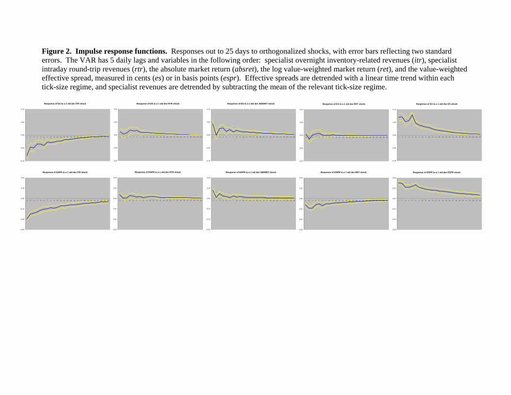
Figure 2. Impulse response functions. Responses out to 25 days to orthogonalized shocks, with error bars reflecting two standard errors. The VAR has 5 daily lags and variables in the following order: specialist overnight inventory-related revenues (itr), specialist intraday round-trip revenues (rtr), the absolute market return (absret), the log value-weighted market return (ret), and the value-weighted effective spread, measured in cents (es) or in basis points (espr). Effective spreads are detrended with a linear time trend within each tick-size regime, and specialist revenues are detrended by subtracting the mean of the relevant tick-size regime. Response of ES to a 1 std dev ITR shock
-0.10
-0.05
0.00
0.05
0.10
1 2 3 4 5 6 7 8 9 10 11 12 13 14 15 16 17 18 19 20 21 22 23 24 25
Response of ES to a 1 std dev ABSRET shock
-0.10
-0.05
0.00
0.05
0.10
1 2 3 4 5 6 7 8 9 10 11 12 13 14 15 16 17 18 19 20 21 22 23 24 25
Response of ES to a 1 std dev RTR shock
-0.10
-0.05
0.00
0.05
0.10
1 2 3 4 5 6 7 8 9 10 11 12 13 14 15 16 17 18 19 20 21 22 23 24 25
Response of ES to a 1 std dev ES shock
-0.10
-0.05
0.00
0.05
0.10
1 2 3 4 5 6 7 8 9 10 11 12 13 14 15 16 17 18 19 20 21 22 23 24 25
Response of ES to a 1 std dev RET shock
-0.10
-0.05
0.00
0.05
0.10
1 2 3 4 5 6 7 8 9 10 11 12 13 14 15 16 17 18 19 20 21 22 23 24 25
Response of ESPR to a 1 std dev RTR shock
-0.30
-0.20
-0.10
0.00
0.10
0.20
1 2 3 4 5 6 7 8 9 10 11 12 13 14 15 16 17 18 19 20 21 22 23 24 25
Response of ESPR to a 1 std dev ABSRET shock
-0.30
-0.20
-0.10
0.00
0.10
0.20
1 2 3 4 5 6 7 8 9 10 11 12 13 14 15 16 17 18 19 20 21 22 23 24 25
Response of ESPR to a 1 std dev RET shock
-0.30
-0.20
-0.10
0.00
0.10
0.20
1 2 3 4 5 6 7 8 9 10 11 12 13 14 15 16 17 18 19 20 21 22 23 24 25
Response of ESPR to a 1 std dev ITR shock
-0.30
-0.20
-0.10
0.00
0.10
0.20
1 2 3 4 5 6 7 8 9 10 11 12 13 14 15 16 17 18 19 20 21 22 23 24 25
Response of ESPR to a 1 std dev ESPR shock
-0.30
-0.20
-0.10
0.00
0.10
0.20
1 2 3 4 5 6 7 8 9 10 11 12 13 14 15 16 17 18 19 20 21 22 23 24 25
Recommended