1
MAGNETOTELLURICS FOR ONSHORE PETROLEUM EXPLORATION: A
CASE STUDY FROM THE OFFICER BASIN
Clarke Petrick
Continental Evolution Research Group
School of Earth and Environmental Sciences
University of Adelaide
Adelaide SA 5005 Australia
Phone: 0408 859 534
Facsimile: 08 83034347
Graham Heinson
Continental Evolution Research Group
School of Earth and Environmental Sciences
University of Adelaide
Adelaide SA 5005 Australia
Phone: 08 83035377
Facsimilie: 08 83034347
E-mail: [email protected]
Left Running Heading: Petrick and Heinson
Right Running Heading: MT Exploration of Officer Basin

2
Table of Contents ABSTRACT……………………………………………………………………………...3
INTRODUCTION……………………………………………………………………….4
GEOLOGICAL SETTING...……………………………………………………………5
MAGNETOTELLURIC EXPLORATION……………….…………………………....6
OFFICER BASIN GEOPHYSICAL EXPLORATION……………………………….7
2D Seismic Lines…………………………………………………………………7
Magnetotellurics………………………………………………………………… 8
Dimensionality of the Earth……………………………………………………10
FIELD
SURVEY………………………………………………………………………...11
Two-dimensional Inversion…………………………………………….………14
DISCUSSION OF MODELLING RESULTS………………………………………...16
Magnetotelluric Results………………………………………………………16
Gravity Results………………………………………………………………..19
CONCLUSION……………………………………………………………………...….21
ACKNOWLEDGEMENTS……………………………………………………………21
REFERENCES…………………………………………………………………...……..22
TABLE AND FIGURE CAPTIONS…………………………………………………..27
EQUATIONS………………………………………………………………………..….30
TABLES AND FIGURES……………………………………………………………...30
Table 1: MT site locations 30
Table 2: Gravity readings 31
Figure 1: Reflection seismic 32
Figure 2: Officer Basin map 33
Figure 3: Schematic of Officer Basin 34
Figure 4: Site locations and MT array 35
Figure 5: Line 85 Pseudo-sections 36
Figure 6: Graph resistivity Vs depth 37
Figure 7: Line 86 TM mode 38
Figure 8: Line 85 TM mode 39
Figure 9: Line 85 TE mode 40
Figure 10:Line 85 TE mode, constrained forward model 41
Figure 11: MT modeling sensitivity test 42
Figure 12: Bouguer gravity values and elevations along line 85 43
Figure 13: Gravity model 44
3
ABSTRACT
The Officer Basin, South Australia, is a sedimentary basin that contains several possible
salt diapiric structures that have been partially defined from two-dimensional (2D)
seismic transects. This paper reports a case study to assess the potential of using
magnetotellurics (MT) and gravity data to delineate salt diapiric structures. The study
aimed to develop an economical and low impact technique for greenfields exploration of
basins in which hydrocarbon resources may be structurally controlled by salt tectonics.
Twenty-six MT sites were deployed across two orthogonal transects (seismic lines 85-
0009 and 86-0194), one that crosses a known salt structure and the other with no salt wall
structure. For the line 85-0009, the depth to the top of the salt dome was 700 m with a
width 2.5 km, and appears to be quite disseminated resulting in low acoustic impedance
contrasts. Each 18 km line was two-dimensionally modeled to a depth of 3.5 km and
evaluated against the seismically imaged basin model.
We show that the salt diapiric structure is only marginally defined by the MT and gravity
data, but with more sites and better quality data the resolution will undoubtedly improve.
The salt structure was imaged in the same location as the seismic anomaly, and appears
as a slightly more resistive body (>200 .m) compared to the porous sedimentary host
(~2-200 .m). The resistivity model imaged the depth of the dipping basement, and is
consistent with the gravity data. We conclude that in areas of salt structure poorly
imaged by seismic methods, MT may be a significant new exploration tool to delineate
potential targets.

4
Key words: Gravity, Magnetotellurics, Officer Basin, Petroleum Exploration, Salt
Diapir.
INTRODUCTION
Petroleum exploration in the Officer Basin began in the 1960s with seismics,
aeromagnetics and regional gravity surveys being carried out (Morton and Drexel, 1997).
Exploration has been sporadic since then, but over 7000 km of 2D seismic data have now
been acquired. Seven petroleum wells and forty-two stratigraphic/deep mineral wells
have also been drilled into the Officer Basin, with indication the presence of a deposit.
However, to date, no significant oil plays have been discovered. Despite the relatively
low levels of exploration in this onshore basin, the petroleum industry in general is yet to
make a judgment on the prospectivity of the Officer Basin (Morton, 1996a).
Much of the 2D seismic imaging in the area is of poor quality. Carbonates commonly
pose difficulties for seismic reflection surveys because excessive reverberations
effectively mask reflections from structures beneath them (Figure 1). Alternative
techniques need to be incorporated to reduce the ambiguities in the interpretation of 2D
seismic reflection data. The MT experiment presented in this paper was carried out
during July-August 2004, and was designed to test the feasibility of MT to delineate the
structure of a salt diapirs identified from a 2D seismic survey. The field area is within the
eastern Officer Basin, which is located in remote western South Australia (Figure 2).

5
GEOLOGICAL SETTING
The Officer Basin is Australia’s largest present day intracratonic basin (Lindsay and
Leven, 1996). The elongate, roughly E-W- trending trough is located in the west of South
Australia and extends into Western Australia. The Neoproterozoic to Palaeozoic basin
was one of a number of troughs that formerly comprised the Centralian Superbasin
(Walter et al., 1995). During the Petermann Orogeny the Centralian Superbasin
dismembered into a southern fragment (Officer Basin), and a northern fragment
(incorporating the Amadeus, Georgina, Ngalia and Savory Basins) (Haddad et al., 2001;
Hoskins and Lemon, 1995; Lindsay and Leven, 1996; Moussavi-Harami and Gravestock,
1995; Walter et al., 1995). The Officer Basin’s northern margin is sharply thrust faulted
against the exhumed Musgrave Block (Walter and Gorter, 1994). Archaean-
Palaeoproterozoic Gawler Craton constrains the basin to the south. The sedimentary
sequences found in the Officer Basin were deposited over 500 Ma, from the initial
deposition of the Willouran (800 Ma), They comprise shallow-water sediments that were
deposited in an extensive sag basin (Preiss and Forbes, 1981; Walter et al., 1992). Three
orogenic events then followed, the Petermann Range Orogeny at 550 Ma (Comacho and
McDougall, 2000; Lindsay and Leven, 1996); the Delamerian Orogeny 500 Ma (Hand et
al., 1999); and finally the Alice Springs Orogeny at 300-400 Ma (Cartwright and Buick,
1999; Hand et al., 1999). The intracratonic thrusting and uplift resulted in the deposition
of thick sedimentary sequences, ending in the Carboniferous (Moussavi-Harami and
Gravestock, 1995).
A marine shelf-evaporitic sea, depositional setting contributed large volumes of salt into
the basin. The intrusion of deep-seated evaporites into overlying sediments may form a

6
structural or stratigraphic hydrocarbon trap. Commercially important traps are
commonly found in sediments associated with rock-salt intrusion (Levorsen, 1967). Salt
can have either an active or passive role in its association with petroleum traps.
Deformation of sediments enclosing the salt dome is caused by active intrusion of the
rising salt mass and subsequent uplifting of adjacent strata (Levorsen, 1967). The source
of the salt in the intrusive salt dome is deep-seated, and has developed into salt walls and
salt pillows, as shown in Figure 3. Both active and passive salt structures have the
potential to form petroleum traps and are actively explored worldwide for this reason
(Lerche and O'Brien, 1987).
MAGNETOTELLURIC EXPLORATION
Magnetotelluric methods may be particularly useful in petroleum exploration for
situations where the seismic technique fails to image sediment packages beneath rock
units that scatter and reflect incident seismic energy (Hoversten et al., 1998). In areas of
difficult terrain, such as the Officer Basin MT methods are cheaper and easier to
undertake than seismic methods (Cull and Gray, 1989). (Constable et al., 1998;
Hoversten et al., 2000) have shown that MT is an increasingly important tool in exploring
offshore sedimentary basins. However, little work has been carried out onshore. A
similar 1D study was conducted in 1989 over the Eromanga Basin, MT inversions
imaged sediment compaction but the results where inconclusive (Cull and Gray, 1989).
In the case of the 100,000 km2 Officer Basin, 2D MT methods may be useful for

7
determining structural relationships, thickness of sedimentary units and the presence of
conductive or resistive masses.
Long-period MT records natural variations of electric and magnetic fields in the band
with of 1 to 105 s. Such data constrain lithospheric-scale structure (Heinson, 1999;
Heinson et al., 1996). However, a marine test above the Gemini structure, Gulf of
Mexico, using magnetic sensors with much higher precision, demonstrated that high-
quality shallow sea-floor MT data could be acquired, despite the attenuation of naturally
occurring fields by electrically conductive seawater (Hoversten et al., 2000). Various
model studies have now been carried out to test the feasibility of the MT method to map
salt bodies in the Gulf of Mexico (Blood, 2001; Hoversten, 1992; Hoversten et al., 1998;
Hoversten and Unsworth, 1994). The resistivity of crystalline salt (>100 .m) is at least
ten times greater than surrounding porous sediments (<10 .m), providing a highly
suitable target for MT (Constable et al., 1998). Hoversten et al. (2000) showed that with
MT data of reasonable quality in the 10-3
to 1Hz (1 to 103 s) band, combined with a
knowledge of the depth to the top of salt, the base of salt could be mapped.
OFFICER BASIN GEOPHYSICAL EXPLORATION
2D Seismic Lines
Extensive 2D seismic surveys have been conducted in the Officer Basin (Morton and
Drexel, 1997). Much of the seismic data produced low-quality images due to the vintage
of processing, energy source and high reflectivity contrasts within the sediments,
8
resulting from the presence of carbonates, crystalline salt (Hoversten et al., 2000).
Excessive reverberations within these units mask signals from deeper reflectors (Ogilive
and Purnell, 1996). The presence of salt with a density () of 2.2 kgm-2
(Blood, 2001) and
a seismic compressional velocity 4500 ms-1
(Telford et al., 1998) creates reflection
coefficients at its boundary of R=+0.176 in a typical sedimentary profile.
Petty-Ray Geophysical Pty Ltd shot line 85-0009 in 1985 with thumper trucks, to a
stacking of 60 fold. Data were then migrated by Hosking Geophysics Corp for Comalco
Mineral and Petroleum Exploration. The inferred salt structure runs east-west,
perpendicular to the series of north-south seismic lines that intercept it. From the series
of 2D seismic transects the width was constrained to be 3.5 km and the length to 12 km.
A number of continuous reflectors have been mapped as horizons, further constrained by
well logging information. Figure 1 shows an example of the data quality from line 85-
0009. The image does not illustrate the typical strong top of salt reflectivity seen in the
Gulf of Mexico (O'Brien and Gray, 1996). Instead, the area had been identified due to
poor reflections and the upward warping of bedding.
Basement in Figure 1 was identified at 1.2 s TWT in the south and 1.8 TWT in the north,
representing a 2 slope to the north. Shallowing of the basin in the south is consistent
with trends observed in gravity data (Haddad et al., 2001). Basement depth at the base of
the salt dome in about 2.6 km and the interpreted top of salt is at a depth of 700 m. This
depth of salt represents maximum dimensions of 2 km in height; a width of 2.5 km and
12 km in length developing a maximum salt affected volume of 20 km3.

9
Magnetotellurics
The MT method utilises natural sources of time-varying magnetic fields that induce
electric current flow in the Earth. Such fluctuations occur over periods from seconds to
hours (Keller and Frischknecht, 1966) The periodicity and polarisation of the inducing
field is not predictable, but times of heightened EM signals can be predicted by
monitoring of solar flare activity. At low frequencies, natural MT fields consist of
periodic variations in Earth’s magnetic field. Such variations arise from interactions
between particle emissions from the Sun and the Earth’s atmosphere and magnetosphere.
Magnetic storms, caused by material ejected from flares on the surface of the sun, occur
approximately once a month and cause erratic variations in the MT field (Vozoff, 1991).
When the flare material enters the Earth’s natural magnetic field it induces a current in
the earth. The horizontal component of the Earth’s magnetic field enhances on the side
facing the solar flare cloud due to the Earth’s Solar diurnal current (Keller and
Frischknecht, 1966). Inducing magnetic events are worldwide, so it is reasonable to treat
the MT field at mid-latitudes as a plane-wave source-field.
Computation of the Earth’s electrical impedance Z from measurements of orthogonal
magnetic (magneto) field B and electric (or telluric) field E yields frequency (period)
dependent responses. Time-series data are Fourier transformed to give expressions of
apparent resistivity (a) and phase () for each period. These two quantities, measured at
a number of locations, are interpreted in terms of the electrical resistivity distribution of
the earth as a function of depth. The MT method depends on the penetration of EM
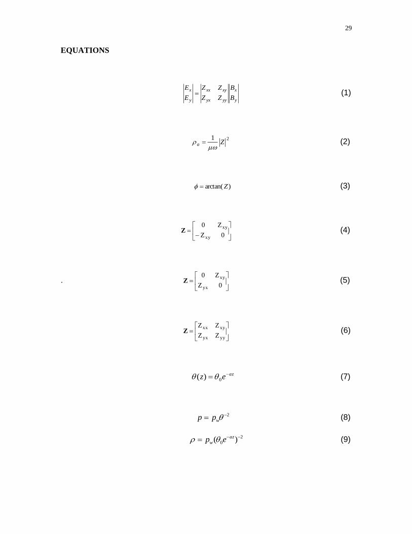
energy into the Earth. The MT impedance tensor Z is defined by:

10
y
x
yyyx
xyxx
y
x
B
B
ZZ
ZZ
E
E (1)
Equation (1) states that B is the inducing field, E the resulting field and Zij represent the
Earth’s electrical impedance.
The apparent resistivity, a, of the conductor can be determined from the equation:
21
Za
(2)
Phase is defined from the equation:
)arctan( Z (3)
Dimensionality of the Earth
In modelling the sub-surface electrical structure, we must consider how the resistivity
varies vertically and laterally. For the trivial case of a homogenous Earth, a is the same
at every frequency, and E leads B in-phase by 45 degrees at all frequencies (Keller and
Frischknecht, 1966). In the real non-homogenous case, the phase relation between the
two field components varies, and determines the Earth’s resistivity distribution (Keller
and Frischknecht, 1966). The 1D case depends only on the change in with depth. In
2−D, resistivity varies along one horizontal coordinate across strike and with depth.
When resistivity varies with both horizontal coordinates and depth the full 3D structure is
displayed (Vozoff, 1991).

11
For a one-dimensional Earth; Zxx = Zyy = 0 and Zxy = Zyx,
0Z
Z0
xy
xyZ (4)
Modeling in two dimensions, the x- axis can be mathematically rotated so that it is
oriented perpendicular to the strike, allowing the impedance values, Zxx Zyy Zxy Zyx
0 to be simplified. Two-dimensional impedance values can be written as Zxx =Zyy=0
and Zxy Zyx 0, giving:
0Z
Z0
yx
xyZ (5)
For a three-dimensional Earth, Zxx Zyy Zxy Zyx 0, and thus
yyyx
xyxx
ZZ
ZZZ (6)
Dimensionality is important because the MT method is sensitive to both structure and
electrical resistivity. In a 2D situation, the Transverse Magnetic (TM) mode defines the
electric field perpendicular and magnetic field parallel to geological strike. Transverse
Electric (TE) mode defines the electric field parallel and the magnetic field
perpendicular. These modes are treated independently; TM mode has components E
(perpendicular), E (vertical) and B (parallel); TE mode has components E (parallel), B
(perpendicular) and B (vertical) (Vozoff, 1972).
FIELD SURVEY
Recent advances in processing and modelling techniques have significantly improved the
MT method and its ease of use. The addition of the remote-reference field reduced noise

12
in magnetic-field measurements (Gamble et al., 1979). Various robust response function
estimation methods have increased the accuracy and certainty of data processing (Chave
et al., 1987; Egbert, 1997; Egbert and Booker, 1986). Development of 1D, 2D and 3D
forward and inverse modelling codes e.g. (Constable et al., 1987; Rodi and Mackie, 2001;
Smith and Booker, 1991; Wannamaker et al., 1986) have produced unprecedented
modelling capabilities.
In the Officer Basin study, MT data were collected with five instruments. Each
instrument comprised a three-component fluxgate magnetometer measuring Bx, By and
Bz and an electrode array which measured Ex and Ey components. The north-south and
east-west electrodes where reduced in length from 50 m to 10 m. The system
configuration is illustrated in Figure 4. This alteration of equipment was performed in the
field to reduce the voltage potential difference between electrodes. Due to the
heterogeneous nature of the sedimentary basin, self-potential (SP) effects generated large
voltage differences, which were off-scale for the recording instrument.
The reduction in dipole length reduced deployment time significantly. Copper sulphate
electrolyte-filled pots were used as electrodes and auguring approximately 50 cm into
moist sand attained good ground coupling. The on-board computer was set running by a
notebook PC with a USB connection to record the signal amplitude at 10 Hz. Each
instrument and electrode was buried to a depth of 20 cm below the surface in an attempt
to stabilize instrument temperature. However, the arid climate produced daily
temperature fluctuations of 30C. This cyclic variation generated a large electrode offset
drift, and in some cases causing voltages to go off-scale. The five instruments were

13
deployed concurrently to facilitate remote referencing between stations (Gamble et al.,
1979).
During each survey, time series of the horizontal electric and magnetic fields were
collected simultaneously over five sites. Magnetotelluric responses in the bandwidth of
10-1000s where recorded over 24 hours at each location. The data recorded showed low-
levels of signal, due to low-levels of natural time-varying magnetic fields present during
the survey period, as noted form the Alice Springs magnetic observatory. A profile of
stations was used to image the lateral extent of the body. Two perpendicular lines where
selected; 85-0009 (line 85) with a salt structure present and 86-0104 (line 86) without
(Figure 4). A site spacing of 1 km was generally used, but some in-filling sites were
added, depending on the complexity of structure interpreted from seismic data.
The raw data, initially in binary format, were converted to ASCII files at four-second
averages, and MT transfer functions were determined using the RRRMT method by
(Chave and Thomson, 1989; Chave et al., 1987). Impedance tensors estimates were
calculated for each site over a band width of 10-1000 s. Data was imported into
WinGLink program and then modeled using 2-D inversion software (Rodi and Mackie,
2001).
Figure 5 displays MT data as a mode pseudo section for line 85. The pseudo-sections
show apparent resistivity in (.m) and phase (in degrees) plotted against period (s) for
the TM mode (upper two plots) and TE mode (lower two plots).
14
In general the resistivity increases from low values at short periods to high values at long
periods, The broad increase in apparent resistivity (particularly in the TM mode) in the
period band of 10 to 100 s below sites I, J and K shows the measured response from the
elevated resistivity of the salt dome. Phase angles are less sensitive to structure and are
rather more homogeneous.
Two-dimensional Inversion
The 2D inversion process involves a smooth model inversion routine developed by (Rodi
and Mackie, 2001) The routine finds regularized solutions (Tikhonov Regularization) to
the 2D-inversion problem for MT data using the method of non-linear conjugate
gradients. The forward model simulations are computed using finite-difference equations
generated by network analogs to Maxwell’s equations. The program inverts for a user-
defined 2D mesh of resistivity blocks, extending beyond the dimensions of the survey
area.
Two profiles were constructed for lines 85 and 86. Both lines intercept at a common site
(A) allowing the lines to be tied see (Figure 4). Not all the MT survey sites were included
in the inversion, due to low coherency values and hence large error bars. Thus 14 sites
were used for line 85. The north-orientated horizontal electrical channel (Ex) or (TM
mode) was input into the inversion algorithm. This channel ran perpendicular to the strike
of the salt structure and should record the greatest level of complexity (Wannamaker,
1984). A bandwidth of 0.1-0.0001 Hz (period of 10-1000 s) was selected from the TM
mode. A number of smooth MT inversions where run over the 85 line. The starting model
in each case was varied between a conductive half space, resistive half space and

15
seismically constrained models. After 300-600 iterations these models converged to a
similar structure. Multiple paths where taken to reach the regional minimum reducing the
possibility of the program locating the RMS in a local minimum. Floor-errors were
applied to data so an error bar of at least 5% surrounded each point at every frequency to
reduce the program over fitting individual points.
The resistivity profile produced from the MT inversion has a causal link with sediment
porosity variations with depth (Heinson and Segawa, 1995). The large connected pore
spaces of the surface sands reduce in porosity lower in the profile due to increased
compaction (Keller and Frischknecht, 1966). Water filled porosity () of sediments can
be related to depth of burial (Z) by a simple exponential function,
azez 0)( (7)
Combining this equation with Archie’s law gives:
2 wpp (8)
2
0 )( az
w ep (9)
The porosity 0 of the sediments in generally 50% at the surface, with ground water
resistivity of 1 . A value of 1.8 km was used for the constant 1a from (Le Pichon et
al., 1990). Figure 6 illustrates the relationship between resistivity and depth that would
be expected due to compaction down to the basement. Indicative salt and basement
resistivities are also displayed showing the level of contrast with surrounding sediments.
Salt has its greatest contrast with sediments at 1 km depth. The sharp change in colour in
the MT images at the basement level concurs with offset in the resistivity along the
dashed line in Figure 6.

16
DISCUSSION OF MODELLING RESULTS
Magnetotelluric Results
The Lines 85 and 86 were modeled in all permutations of TM, TE and vertical field (Hz)
modes with a consistent model of increasing resistivity down to the dipping basement.
From all these, three representative images with low RMS have been presented (Figure
7,8 and 9).
Line 86 was imaged in TM mode in an attempt to depict any structures (Figure 7). No
significant anomalies were observed from the data in either pseudo-sections or in the TE
modes. Figure 7 shows vertically increasing resistivity, with almost no lateral variation,
consistent with a sedimentary profile from an extensional basin (Keller and Frischknecht,
1966). The result from this line accurately represented the horizontal structure of basin
along strike with a shallow dip to the west, interpreted from seismic, gravity and basin
evolution models (Morton and Drexel, 1997).
Line 85 is of great interest and shows a resistivity deviation from the norm in the TM
mode (Figure 8). An increase in resistivity below stations I J and K is coincident with
inferred salt from seismic imaging. Presence of this feature is not as clear in the TE
mode (Figure 9), as the structure is orientated parallel to the electric dipole in this mode,
and there would be little electric field change along strike (Wannamaker, 1984).
However, the basement structure (> 1000 .m), which is laterally extensive, has been

17
well modelled in both modes. Interestingly a slight rise in the basement below site M
coincides with a salt withdrawal zone interpreted by (Lindsay and Leven, 1996).
A limitation of MT modelling is that it represents resistivity as an averaging of the earth’s
true resistivity, reducing the definition of any structure observed. Modelling also works
on a smoothing factor, further reducing anomalous features and fitting them to a simpler
model. The contrast between porous saturated sediments (1-20 .m) and salt (100
.m) provides an order of magnitude contrast, but this can be overwhelmed by
difference of two orders of magnitude between the sediments and basement (1000 .m)
which is much more prominent.
The non-uniqueness of MT provides a high level of variability and allows a number of
possible geological interpretations. Additional information can quickly constrain the
model. Seismic distortion is indicative of a salt presence. The presence at depth of the
the evaporite Alinya Formation (Figure 1) provides a source of salt to explain the
resistive anomaly. The salt structure could be a salt wall, or a salt migration.
The salt wall hypothesis was tested using a seismically defined forward model. The
basement architecture was maintained from Figures 8 and 9 which were already
consistent with seismic data. A pillar of resistivity 100 .m was drawn in to represent a
salt dome. The model was run for 100 iterations in the TM mode. The smoothing factor
was reduced for the inversions so as to maintain as much structure as possible. The salt
structure presence was maintained after 100 iterations and little variation was seen in the
basement (Figure 10). The RMS (1.277) recorded was slightly lower than in Figures 8

18
and 9, which was recorded from the unconstrained model. The resistivity high on the
basement is reduced in Figure 8, and the resistivity in the zone of salt dome is increased.
This is due the non-uniqueness of MT and the number of local minimums. The result is
an accurate model consistent with the seismic salt wall interpretation produced by PIRSA
(2000).
As a test of model sensitivity, a second identical salt structure was placed under site G in
Figure 11. The structure was inconsistent with existing seismic data to test the sensitivity
of the model to this structure, under the same conditions as in the previous salt dome
forward model (Figure 10). Figure 11 illustrates the model after 100 iterations. We note
that the second salt dome is not preserved in the inversion, and is therefore not required
by the TM mode data. The lower figure indicates model sensitivity, with blue regions
showing maximum sensitivity and red low sensitivity. There is good sensitivity directly
beneath sites I, J and K indicating that we have confidence that the salt wall is required
part of the model.
The region of salt was not as clearly imaged as for other salt bodies in the Gulf of Mexico
(Constable et al., 1998). We suggest that the the salt is widely disseminated. This would
explain the low level of resistive contrast and the absence of a strong reflection from the
top of the salt structure.
An interpretation of Figure 7 was conducted independent of existing basin knowledge. A
salt roller model can be used to explaine the resistivity result, because salt migrates, it
forms laterally extensive salt bands (Guglielmo et al., 1997). This is the simplest

19
explanation and would be the case if MT were the sole exploration tool. It can be seen
from seismic that the edges of the affected area are vertical and the displacement of
reflector is greater than that of the salt roller accumulation. The salt structure does not
display the lateral branching or relay patterns of the seismic roller model (Guglielmo et
al., 1997).
Gravity Results
The gravity profile along line 85 was taken at 500 m intervals with a La Coste Romberg
Gravimeter (Figure 4). Bouguer gravity anomalys were calculated accounting for a free
air corrections, instrumental drift and Bouguer slab. It must be noted that due to the trial
nature of the survey, latitude corrections and terrain were not performed. Elevations
were inferred from seismic shot point locations to an accuracy of 1 m (Figure 12). Sand
dunes over the survey line had been mobile since they were first recorded in 1985. Due
to this fact and the interpolation of elevation between seismic recordings, errors were
increased to 2.5 m. This uncertainty was included into free air and Bouguer corrections
and represent an underlying 0.5 mGal uncertainty.
A 20 mGal slope across the profile was delineated confirming the increased basement
depth to the north and the filing of younger sediments of lower density (Haddad et al.,
2001). The dipping basin and sedimentary profile was modelled to a depth of 10 km
(Figure 12). A small -3 mGal gravity anomaly at site K (location E788386 N6868774)
overlies the salt body. Modelling of gravity profile in Model Vision 5.0 shows that the
body can be represented as a body of slightly lower density putting further constraint on
20
the overall interpretation. However due to the accuracy of gravity data, further inferences
were not possible.
Imaging of comparative densities between pure salt and surrounding sediment can be
constrained in modelling by assigning known values of salt. Crystalline salt has a density
2.2 g/cm3 that remains constant under increasing pressure, unlike sediments which
increases as a function of depth due to compaction. An estimation of concentration is
needed in the contaminated-salt block case. Assuming 80% salt at 2.2 g/cm3
and 20%
anhydrite at 2.90 g/cm3 a density of 2.34 g/cm
3 is produced. This ratio has been
successful in gravity modelling in the South Oman basin (Blood, 2001). The volume and
depth of salt can be calculated from gravity modelling, but density values of the
surrounding sediments must be constrained (Smith & Whitehead, 1989). This can be
calculated from base line gravity response, using density wireline log well data or
estimations of compaction rates. Regional variations in geology make the identification
of small negative amplitude anomalies extremely difficult; a feature also reported by
Smith and Whitehead (1989). Closely spaced gravity measurements have, however,
identified basement and, indicate the possible presence of salt. The size of the salt dome
has made identification difficult. It has been stated that a salt body of dimensions greater
than 5 km is needed amongst compacted sediments to be resolved independently by
gravity (Blood, 2001).
21
CONCLUSION
MT has proven itself as a significant geophysical technique for the onshore investigation
of subsurface salt structure in sedimentary basins. Resistivity model studies have
independently imaged 1000 .m resistive basement over two profiles at a depth of 2.5
km. Sedimentary sequence resistivities were shown to increase down the profile.
Calculations of porosity variation with depth produced matching resistivities.
Identification of elevated resistivities were depicted, and are associated with salt bodies.
With the addition of seismic data MT modelling allowed the resistivity and dimensions to
be further constrained to 100 .m to a depth of 700 m and a width of 2.5 km. The
seismically-constrained salt wall interpretation was confirmed with a reduction in misfit.
The MT method is a cheap and effective approach for mapping salt onshore. Minimal
environmental impact, remote access and low logistical requirements are all
characteristics that make MT a unique deep exploration technique for areas that have
poor seismic coverage. Development of sites over existing seismic profiles allows higher
confidence in interpretation. Quality of data could be significantly enhanced with
additional instruments, closer spaced deployments and an increase in recording time.
ACKNOWLEDGEMENTS
Special thanks go to my supervisor, Dr Graham Heinson for dedicating his time and
knowledge to this endeavour. I would like to thank Dr Peter Boult and PIRSA for
developing and financially supporting this project. Gratitude also goes to the ASEG
Research Foundation for their financial assistance. Adam Davey, Oliver Ninglegen,
22
Dennis Rippe and Stephan Thiel were essential participants during expeditions to the
Officer Basin. We wish to thank the Maralinga Tjarutja for permitting access to their
land.
REFERENCES
Blood, M. F., 2001, Exploration for a frontier salt basin in Southwest Oman: The Leading
Edge, 20, 1252.
Carter, N. L. and Hanansen, F. D., 1983, Creep of rock salt: Tectonophysics, 116, 275-
333.
Cartwright, I. and Buick, I. S., 1999, The flow of surface derived fluids through Alice
Springs age middle-crustal ductile shear zones, Reynolds Range, central Australia:
Journal of Metamorphic Geology, 17, 397-414.
Chave, A. D. and Thomson, D. J., 1989, Some comments on magnetotelluric response
function estimation: Journal of Geophysical Research, 94, 14215-14225.
Chave, A. D., Thomson, D. J. and Ander, M. E., 1987, On the robust estimation of power
spectra, coherences, and transfer functions: Journal of Geophysical Research, 92, 633-
648.
Comacho, A. and McDougall, I., 2000, Intracratonic strike-slip partitoned transpression
and the formation and exhumation of eclogite facies rocks: an example from the
Musgrave Block, central Australia: Tectonics, 19, 978-996.
Constable, S. C., Orange, A. S., Hoversten, G. M. and Morrison, H. F., 1998, Marine
magnetotellurics for petroleum exploration Part I: A sea-floor equipment system:
Geophysics, 63, 816-825.
Cull, J. P. and Gray, J. D., 1989, Sedimentary Compaction and Magnetotelluric Data in
the Eromanga Basin: Exploration Geophysics, 20, 335-337.
Egbert, G. D., 1997, Robust multiple-station magnetoturic data processing: Geophysics
Journal of the royal Astronomical Society , 130, 475-496.
Egbert, G. D. and Booker, J. R., 1986, Robust estimation of geomagnetic transfer
functions: Geophysics, 87, 173-194.
23
Gamble, T. D., Goubau, W. M. and Clarke, J., 1979, Magnetotellurics with remote
magnetic reference: Geophysics, 44, 53-68.
Guglielmo, G., Jackson, J. M. P. A. and Vendeville, B. C., 1997, Three-dimensional
visualization of salt walls and associated fault systems: AAPG Bulletin, 81, 46-61.
Haddad, D., Watts, A. B. and Lindsay, J., 2001, Evolution of the intracratonic Officer
Basin, central Australia: implications from subsidence analysis and gravity modelling:
Basin Research, 13, (217-238).
Hand, M., Mawby, J., Kinny, P. and Foden, J., 1999, U-Pb ages from the Hart's Range,
central Australia: evidence for early Ordovician extention and constraints on
Carboniferous metamorphism: Journal of Geological Society, London, 156, 715-730.
Heinson, G. and Segawa, J., 1995, Electrokinetic signature of the Nankai Trough
accretionary complex: preliminary modelling for the Kaiko-Tokai program: Physics of
the Earth and Planetary Interiors, 99, 33-53.
Hoskins, D. and Lemon, N., 1995, Tectonic development of the eastern Officer Basin,
central Australia: Exploration Geophysics, 26, 243-246.
Hoversten, G. M., 1992, Seaborne electromagnetic subsalt exploration: EOS, 73, 313.
Hoversten, G. M., Morrison, H. F. and Constable, S. C., 1998, Marine magnetotellurics
for petroleum exploration, Part II: Numerical analysis of subsalt resolution: Geophysics,
63, 826-840.
Hoversten, M. G., Constable, S. C. and H., M. F., 2000, Marine magnetotellurics for
base-of-salt mapping: Gulf of Mexico field test at the Gemini structure: Geophysics, 65,
1476-1488.
Keller, G. V. and Frischknecht, F. C., 1966, Electrical Methods in Geophysical
Prospecting, Pergamon Press, Inc.
Le Pichon, X., Henry, P. and Lallemant, S., 1990, Water flow in the Barbados
Accretionary Complex: Geophysical Research, 95, 8945-8967.
Lindsay, J. F. and Leven, J. H., 1996, Evolution of a Neoproterozoic to Palaeozoic
intracratonic setting, Officer Basin South Australia: Basin Research, 8, 403-424.
Levorsen, A.I., 1967, Geology of Petroleum, 2nd Edition. publisher, Freeman, W.H. &
Co.
Lerche, I. and O'Brien, J. J., 1987, Dynamic geology of salt and related structures,
published Academic Press, Inc.
Morton, J. G. G., 1996, MESA Petroleum industry survey: South Australian. Department
of Mines and Energy report book, 96, 17-63.

24
Morton, J. G. G. and Drexel J. F, 1997, The Petroleum Geology Of South Australia,
Volume 3: Officer Basin, 1-321.
Moussavi-Harami, R. and Gravestock, D. I., 1995, Burial history of the eastern Officer
Basin, South Australia: AAPG Journal, 35, 307-320.
O'Brien, M. J. and Gray, S. H., 1996, Can we image beneath salt?: The Leading Edge, 15,
Ogilive, J. S. and Purnell, G. W., 1996, Effects of salt-related mode conversion on subsalt
prospecting: Geophysics, 61, 331-348.
Preiss, W. V. and Forbes, B. G., 1981, Stratigraphy, correlaion and sedimentary history
of Adeladiean (Late Proterozoic) basins in Australia: Precambrian Research, 15, 255-
304.
PIRSA, 2002, Officer Basin, Primary Industries and Resourses South Australia, 1-13.
Rodi, W. and Mackie, R. L., 2001, Nonlinear conjugate gradients algorithm for 2-D
magnetotelluric inversion: Geophysics, 66, 174-187.
Smith, J. T. and Booker, J. R., 1991, Rapid inversion of two and three-dimensional
magnetotelluric data: Journal of Geophysical Research, 96, 3905-3922.
Vozoff, K., 1972, The magnetotelluric method in exploration of sedimentary basins:
Geophysics, 37, 98-141.
Vozoff, K., 1991, The magnetotelluric method, in Nabighian, M. N., Ed.,
Glectromagnetic methods in applied geophysics, 2: Society of Exploration Geophysists,
641-711.
Walter, M. R., Veevers, J. L., Calver, C. R., Grey, K. and Hilyard, D., 1992, The
Proterozoic Centralian Superbasin: a frountier petroleum province: Bulletin American
Association of Perroleum Geology, 76, 1132.
Walter, M. R., Veevers, J. L., Calver, C. R. and Grey, K., 1995, Neoproterozoic
stratigraphy of the Centralian Superbasin, Australia.: Precambrian Research, 73, 173-
195.
Walter, M. R. and Gorter, J. D., 1994, The Neoproterozoic Centralian Superbasin in
Western Australia. Petroleum Exploration Society Australia, 851-964.
Wannamaker, P. E., Stodt, J. A. and Rijo, L., 1986, A stable finite element solution for
two-dimensional modeling: Geophysics, 37, 277-296.
Smith, J. T. and Booker, J. R., 1991, Rapid inversion of two and three-dimensional
magnetotelluric data: Journal of Geophysical Research, 96, 3905-3922.
25
Telford, W. M., Geldart, L.P. and Sheriff, R. E, 1998, Applied Geophysics Second
edition, Cambridge University Press.
Vozoff, K., 1972, The magnetotelluric method in exploration of sedimentary basins:
Geophysics, 37, 98-141.
Vozoff, K., 1991, The magnetotelluric method, in Nabighian, M. N., Ed.,
Electromagnetic methods in applied geophysics, 2: Society of Exploration Geophysists,
641-711.
Walter, M. R., Veevers, J. L., Calver, C. R. and Grey, K., 1995, Neoproterozoic
stratigraphy of the Centralian Superbasin, Australia.: Precambrian Resurch, 73, 173-195.
Walter, M. R., Veevers, J. L., Calver, C. R., Grey, K. and Hilyard, D., 1992, The
Proterozoic Centralian Superbasin: a frountier petroleum province: Bulliten American
Association of Perroleum Geology, 76, 1132.
Wannamaker, P. E., Stodt, J. A. and Rijo, L., 1986, A stable finite element solution for
two-dimensional modeling: Geophysics, 37, 277-296.
Yilmas, O., 2001, Seismic data analysis. Processing, inversion and interpretation of
seismic data: SEG Investigation in Geophysics, 10, 171-213.

26
TABLES AND FIGURE CAPTIONS
Table 1: MT data recorded in the Officer Basin in July and August 2004. Lines 85 and
86 are aligned north-south and east-west respectively. Site A is the intercept location and
is common to both lines.
Table 2: Gravity data locations and Bouguer gravity calculations. Readings were taken
at approximately 500 m intervals away from topographic highs as to reduce the need for
terrain corrections.
Fig. 1: Reflection seismic data recorded in 1985, a number of horizons have been traced.
The salt dome in question has been outlined in yellow. Adapted from Morton (1997).
Fig. 2: The map of the Officer Basin shows general geology within South Australia. The
darkened square in the center map shows the location of the study area and the
orientation of profiles. Munta 1 well is located on the western end of line 86. Basin depth
increases towards the Manyari Trough. Adapted from PIRSA, (2002).
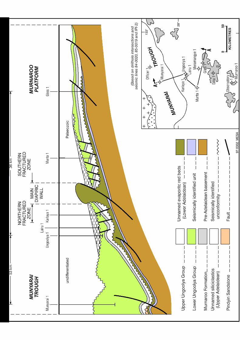
Fig. 3: Schematic cross section of the Officer Basin. The diapric wall is located between
wells Karlaya 1 and Munta 1 is a close representation of seismic line 85. Adapter from
PIRSA, (2002).

27
Fig. 4: Illustrates the site locations of MT and gravity lines with respect to the salt wall.
Site A is common to both lines and Munta 1 is located at site O on line 86. The MT array
shows the instrument deployment.
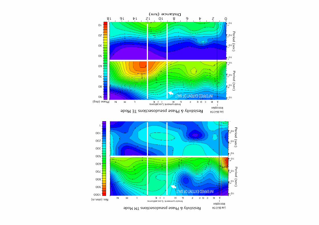
Fig. 5: Line 85 pseudo-sections. The TM mode represents a broad resistive high over the
area of the salt dome. TE mode also displays this anomaly at the surface with an
additional zone of high resistivities at high periods.
Fig. 6: The basin resistivity graph generated from equation (9) shows the change in
resistivity with depth in the sedimentary profile. The dark solid line represents the higher
more homogeneous resistivity of the basement. Triple lines displayed the salt and the
variation of the resistivity contrast with the sediments.
Fig. 7: Line 86 is located along the flank of the salt dome at a distance of 7 km. The MT
model shows the vertical profile and accurately depicts westerly dip in the basement.
The image has been overlaid with reflection seismic data and mapped horizons have been
interpreted from well Munta 1.
Fig. 8: Line 85 crosses the salt dome at locations I, J and K. The MT image shows a
slight resistivity high in the TM mode, along with the basin profile and basement. Below
site B is increased resistively associated with a salt withdrawn zone.

28
Fig. 9: Line 85 was imaged in the TE mode, the same high resistivity bump was not
shown as in Figure 8 but a slight elevation in resistivity at 1 km depth can be observed.
The basement structure was close to that of the TM mode.
Fig. 10: This MT image is the result of 100 iterations of a seismically defined TM
forward mode. The number iterations and a reduction in RMS from Figure 8 gives the
reader confidence in the image. MT has imaged the salt dome extremely close to that
seen in Figure 1.
Fig. 11: Line 85 MT image in TM mode. A reproduction of Figure 10 was carried out
with 2 identical domes, to test the discriminative characteristics of the inversion process.
The result shows a reduction in dome 2 and an increase in RMS error. The sensitivity of
the program with depth shows that both domes are in equivalent zones. The second dome
has been reduces as it doesn’t fit the data.
Fig. 12: Graph of Bouguer gravity at each site location. The lower figure shows 1985
seismic shot point elevations used in gravity calculations. It can be seen that the
instrument elevation has been correctly calculated, as there no correlation between
graphs.
Fig. 13: The gravity model shows dipping basement consistent with the MT figures and
shows a small -3 mGal anomaly above the salt dome.
29
EQUATIONS
y
x
yyyx
xyxx
y
x
B
B
ZZ
ZZ
E
E (1)
21
Za
(2)
)arctan( Z (3)
0Z
Z0
xy
xyZ (4)
.
0Z
Z0
yx
xyZ (5)
yyyx
xyxx
ZZ
ZZZ (6)
azez 0)( (7)
2 wpp (8)
2
0 )( az
w ep (9)


Recommended


![Petroleum (Onshore) Act 1991 · Petroleum (Onshore) Regulation 2016 [NSW] Explanatory note Page 2 Published LW 12 August 2016 (2016 No 500) (q) the certificate of authority required](https://img.pdfslide.us/doc/110x75/5f169642ea28275573224bd6/petroleum-onshore-act-1991-petroleum-onshore-regulation-2016-nsw-explanatory.jpg)