IJMMS 2004:62, 3357–3368PII. S0161171204311270
http://ijmms.hindawi.com© Hindawi Publishing Corp.
MAGNETOHYDRODYNAMICS EFFECT ON THREE-DIMENSIONALVISCOUS INCOMPRESSIBLE FLOW BETWEEN TWO HORIZONTAL
PARALLEL POROUS PLATES AND HEAT TRANSFER WITHPERIODIC INJECTION/SUCTION
PAWAN KUMAR SHARMA and R. C. CHAUDHARY
Received 23 November 2003
We investigate the hydromagnetic effect on viscous incompressible flow between two hor-izontal parallel porous flat plates with transverse sinusoidal injection of the fluid at thestationary plate and its corresponding removal by periodic suction through the plate inuniform motion. The flow becomes three dimensional due to this injection/suction veloc-ity. Approximate solutions are obtained for the flow field, the pressure, the skin-friction, thetemperature field, and the rate of heat transfer. The dependence of solution onM (Hartmannnumber) and λ (injection/suction) is investigated by the graphs and tables.
2000 Mathematics Subject Classification: 76D99, 76W05, 80A20.
1. Introduction. The problem of laminar flow control has become very important
in recent years, particularly in the field of aeronautical engineering, owing to its ap-
plication in reducing drag and hence in enhancing the vehicle power by a substantial
amount. Several methods have been developed for the purpose of artificially controlling
the boundary layer and the developments on this subject. The boundary layer suction
is one of the effective methods of reducing the drag coefficient, which entails large
energy losses. The effect of different arrangements and configurations of the suction
holes and slits has been studied by various scholars. Gersten and Gross [2] have in-
vestigated the flow and heat transfer along a plane wall with periodic suction velocity.
Effects of such a suction velocity on various flow and heat transfer problems along
flat and vertical porous plates have been studied by Singh et al. [10, 11] and Singh [8].
Recently the problem of transpiration cooling with the application of the transverse
sinusoidal injection/suction velocity has been studied by Singh [9].
Magnetic fields influence many natural and man-made flows. They are routinely used
in industry to heat, pump, stir, and levitate liquid metals. There are the terrestrial mag-
netic field, which is maintained by fluid motion in the earth’s core, the solar magnetic
field which generates sunspots and solar flares, and the galactic field which influences
the formation of stars. The flow problems of an electrically conducting fluid under the
influence of magnetic field have attracted the interest of many authors in view of their
applications to geophysics, astrophysics, engineering, and to the boundary layer con-
trol in the field of aerodynamics. On the other hand, in view of the increasing technical
applications using magnetohydrodynamics (MHD) effect, it is desirable to extend many
of the available viscous hydrodynamic solutions to include the effects of magnetic field

3358 P. K. SHARMA AND R. C. CHAUDHARY
for those cases when the viscous fluid is electrically conducting. Rossow [5], Greenspan
and Carrier [3], and Singh [6, 7] have studied extensively the hydromagnetic effects
on the flow past a plate with or without injection/suction. The hydromagnetic chan-
nel flow and temperature field was investigated by Attia and Kotb [1]. Hossain et al.
[4] have studied the MHD free convection flow when the surface is kept at oscillating
surface heat flux. Boundary layer flows of fluids of small electrical conductivity are im-
portant, particularly in the field of aeronautical engineering. Therefore the object of the
present note is to study the effects of the magnetic field on the flow of a viscous, in-
compressible, and electrically conducting fluid between two horizontal parallel porous
plates with transverse sinusoidal injection of the fluid at the stationary plate and its
corresponding removal by periodic suction through the plate in uniform motion.
2. Formulation of the problem. We consider the Couette flow of a viscous incom-
pressible electrically conducting fluid between two parallel flat porous plates with trans-
verse sinusoidal injection of the fluid at the stationary plate and its corresponding re-
moval by periodic suction through the plate in uniform motion U . Let the x∗−z∗ plane
lie along the plates and let the y∗-axis be taken normal to the free-stream velocity. The
distance d is taken between the plates. Denote the velocity components by u∗, v∗, w∗
in the x∗-, y∗-, z∗-directions, respectively. The lower and upper plates are assumed
to be at constant temperature T0 and T1, respectively, with T1 > T0. We derive the gov-
erning equations with the assumption that the flow is steady and laminar, and is of
a finitely conducting fluid. The magnetic field of uniform strength B is applied to the
perpendicular of the free-stream velocity (see Figure 2.1); at lower magnetic Reynolds
number, the magnetic field is practically independent of the flow motion and the in-
duced magnetic field is neglected. The Hall effects, electrical and polarization effects
also have been neglected. All physical quantities are independent of x∗ for this problem
of fully developed laminar flow, but the flow remains three-dimensional due to the in-
jection/suction velocity V∗(z∗)=V(1+εcosπz∗/d). Thus, under these assumptions,
the problem is governed by the following nondimensional system of equations:
vy+wz = 0, (2.1)
vuy+wuz =[uyy+uzz−M2(u−1)
]λ
, (2.2)
vvy+wvz =−py+[vyy+vzz
]λ
, (2.3)
vwy+wwz =−pz+[wyy+wzz−M2w
]λ
, (2.4)
vθy+wθz =(θyy+θzz
)λPr
, (2.5)
where y = y∗/d, z = z∗/d, u= u∗/U , v = v∗/V , w =w∗/V , p = p∗/ρV 2, Pr (Prandtl
number) = ν/α, M (Hartmann number) = (σB2d2/ρν)1/2, λ (injection/suction
parameter) = Vd/ν , and θ = (T∗−T0)/(T1−T0) are the dimensionless quantities and
V , ρ, ν , α, σ , and p are, respectively, injection/suction velocity, density, kinematic

MAGNETOHYDRODYNAMICS EFFECT ON THREE-DIMENSIONAL VISCOUS . . . 3359
y∗
U
V∗(z∗)
V∗(z∗)
x∗
d
B
z∗o
T1
T0
Figure 2.1. Schematic of the flow configuration.
viscosity, thermal diffusivity, electrical conductivity, and pressure. In energy equation
terms corresponding to viscous dissipation and Joule heating have been neglected due
to their small magnitude as compared to other terms. The (∗) stands for dimensional
quantities. The corresponding boundary conditions in the dimensionless form are
y = 0 :u= 0, v(z)= 1+εcosπz, w = 0, θ = 0,
y = 1 :u= 1, v(z)= 1+εcosπz, w = 0, θ = 1.(2.6)
3. Solution of the problem. Since the amplitude of the injection/suction velocity
ε (� 1) is very small, we now assume the solution of the following form:
f(y,z)= f0(y)+εf1(y,z)+ε2(y,z)+··· , (3.1)
where f stands for any of u, v , w, p, and θ. When ε = 0, the problem is reduced to the
well-known two-dimensional flow. The solution of this two-dimensional problem is
u0(y)= 1+[exp
(J2+J1y
)−exp(J1+J2y
)][exp
(J1)−exp
(J2)] ,
θ0(y)=[exp(λPry)−1
][exp(λPr)−1
] , v0 = 1, w0 = 0, p0 = constant,
(3.2)

3360 P. K. SHARMA AND R. C. CHAUDHARY
where
J1 =[λ+(λ2+4M2
)1/2]
2, J2 =
[λ−(λ2+4M2
)1/2]
2. (3.3)
When ε ≠ 0, substituting (3.1) in (2.1)–(2.5) and comparing the coefficient of ε, neglecting
those of ε2,ε3, . . . , the following first-order equations are obtained with the help of
solution (3.2):
v1y+w1z = 0, (3.4)
v1u0y+u1y =(u1yy+u1zz−M2u1
)λ
, (3.5)
v1y =−p1y+(v1yy+v1zz
)λ
, (3.6)
w1y =−p1z+(w1yy+w1zz−M2w1
)λ
, (3.7)
v1θ0y+θ1y =(θ1yy+θ1zz
)λPr
. (3.8)
The corresponding boundary conditions reduce to
y = 0 :u1 = 0, v1 = cosπz, w1 = 0, θ1 = 0,
y = 1 :u1 = 0, v1 = cosπz, w1 = 0, θ1 = 0.(3.9)
This is the set of linear partial differential equations, which describe the three-
dimensional flow. To solve these equations, we assume v1, w1, p1, u1, and θ1 of the
following form:
u1(y,z)=u11(y)cosπz,
v1(y,z)= v11(y)cosπz,
w1(y,z)=−{v′11(y)sinπz
}π
,
p1(y,z)= p11(y)cosπz,
θ1(y,z)= θ11(y)cosπz,
(3.10)
where the prime denotes differentiation with respect to y . Expressions for v1(y,z)and w1(y,z) have been chosen so that the equation of continuity (3.4) is satisfied.
Substituting (3.10) in (3.5)–(3.8) and applying the corresponding boundary conditions,

MAGNETOHYDRODYNAMICS EFFECT ON THREE-DIMENSIONAL VISCOUS . . . 3361
we get the solutions for v1, w1, p1, u1, and θ1 as follows:
v1(y,z)= (A)−1[A1 exp(J3y
)+A2 exp(J4y
)−A3 exp(J5y
)−A4 exp(J6y
)]cosπz,
w1(y,z)=−(πA)−1[A1J3 exp(J3y
)+A2J4 exp(J4y
)−A3J5 exp(J5y
)
−A4J6 exp(J6y
)]sinπz,
p1(y,z)=(π2λA
)−1[A1J3(J1J3−λJ3−M2)exp
(J3y
)+A2J4(J1J4−λJ4−M2)exp
(J4y
)
−A3J5(J2J5−λJ5−M2)exp
(J5y
)
−A4J6(J2J6−λJ6−M2)exp
(J6y
)]cosπz,
u1(y,z)=[E exp
(g1y
)+F exp(g2y
)
+b1
{A1
(J1 exp
(J2+J1y+J3y
)b2
− J2 exp(J1+J2y+J3y
)b6
)
+A2
(J1 exp
(J2+J1y+J4y
)b3
− J2 exp(J1+J2y+J4y
)b7
)
−A3
(J1 exp
(J2+J1y+J5y
)b8
− J2 exp(J1+J2y+J5y
)b4
)
−A4
(J1 exp
(J2+J1y+J6y
)b9
− J2 exp(J1+J2y+J6y
)b5
)}]cosπz,
θ1(y,z)=[Rexp
(s1y
)+S exp(s2y
)
+C1
{A1 exp
(J3y+λPry
)C2
+ A2 exp(J4y+λPry
)C3
− A3 exp(J5y+λPry
)C4
− A4 exp(J6y+λPry
)C5
}]cosπz,
(3.11)
where
A= [J4J5+J3J6−J3J5−J4J6]{
exp(J5+J6
)+exp(J3+J4
)}
−[J4J5+J3J6−J3J4−J5J6]{
exp(J3+J5
)+exp(J4+J6
)}
−[J5J6+J3J4−J3J5−J4J6]{
exp(J3+J6
)+exp(J4+J5
)},
A1 =[J4J6−J5J6
]exp
(J4+J5
)−[J4J5−J5J6]exp
(J4+J6
)+[J4J5−J4J6]exp
(J5+J6
)
+[J4J5−J4J6]exp
(J4)+[J5J6−J4J5
]exp
(J5)+[J4J6−J5J6
]exp
(J6),

3362 P. K. SHARMA AND R. C. CHAUDHARY
A2 =[J3J5−J5J6
]exp
(J3+J6
)−[J3J6−J5J6]exp
(J3+J5
)−[J3J5−J3J6]exp
(J5+J6
)
+[J3J6−J3J5]exp
(J3)+[J3J5−J5J6
]exp
(J5)+[J5J6−J3J6
]exp
(J6),
A3 =[J4J6−J3J6
]exp
(J3+J4
)+[J3J4−J4J6]exp
(J3+J6
)−[J3J4−J3J6]exp
(J4+J6
)
−[J3J4−J3J6]exp
(J3)−[J4J6−J3J4
]exp
(J4)−[J3J6−J4J6
]exp
(J6),
A4 =[J3J5−J4J5
]exp
(J3+J4
)+[J4J5−J3J4]exp
(J3+J5
)−[J3J5−J3J4]exp
(J4+J5
)
−[J3J5−J3J4]exp
(J3)−[J3J4−J4J5
]exp
(J4)−[J4J5−J3J5
]exp
(J5),
J3 =[J1+
(J2
1 +4π2)1/2
]
2, J4 =
[J1−
(J2
1 +4π2)1/2
]
2, J5 =
[J2+
(J2
2 +4π2)1/2
]
2,
J6 =[J2−
(J2
2 +4π2)1/2
]
2, g1 =
[λ+(λ2+4π2+4M2
)1/2]
2,
g2 =[λ−(λ2+4π2+4M2
)1/2]
2, s1 =
[λPr+(λ2Pr2+4π2
)1/2]
2,
s2 =[λPr−(λ2Pr2+4π2
)1/2]
2, b1 = λ[
A{
exp(J1)−exp
(J2)}] ,
b2 = 3J1J3−λJ3, b3 = 3J1J4−λJ4, b4 = 3J2J5−λJ5, b5 = 3J2J6−λJ6,
b6 = 2J2J3+J1J3−λJ3, b7 = 2J2J4+J1J4−λJ4, b8 = 2J1J5+J2J5−λJ5,
b9 = 2J1J6+J2J6−λJ6, C1 = λ2Pr2[A{
exp(λPr)−1}] , C2 = J1J3+J3λPr,
C3 = J1J4+J4λPr, C4 = J2J5+J5λPr, C5 = J2J6+J6λPr,
C6 = λ[A{
exp(J1)−exp
(J2)}·{exp
(g1)−exp
(g2)}] ,
C7 = λ2Pr2[A{
exp(λPr)−1}·{exp
(s1)−exp
(s2)}] ,
E=C6
[A1
{J1(exp
(J2+g2
)−exp(J1+J2+J3
))b2
− J2(exp
(J1+g2
)−exp(J1+J2+J3
))b6
}
+A2
{J1(exp
(J2+g2
)−exp(J1+J2+J4
))b3
−J2(exp
(J1+g2
)−exp(J1+J2+J4
))b7
}
−A3
{J1(exp
(J2+g2
)−exp(J1+J2+J5
))b8
−J2(exp
(J1+g2
)−exp(J1+J2+J5
))b4
}
−A4
{J1(exp
(J2+g2
)−exp(J1+J2+J6
))b9
− J2(exp
(J1+g2
)−exp(J1+J2+J6
))b5
}],

MAGNETOHYDRODYNAMICS EFFECT ON THREE-DIMENSIONAL VISCOUS . . . 3363
F = C6
[A1
{J1(exp
(J1+J2+J3
)−exp(J2+g1
))b2
− J2(exp
(J1+J2+J3
)−exp(J1+g1
))b6
}
+A2
{J1(exp
(J1+J2+J4
)−exp(J2+g1
))b3
− J2(exp
(J1+J2+J4
)−exp(J1+g1
))b7
}
−A3
{J1(exp
(J1+J2+J5
)−exp(J2+g1
))b8
− J2(exp
(J1+J2+J5
)−exp(J1+g1
))b4
}
−A4
{J1(exp
(J1+J2+J6
)−exp(J2+g1
))b9
− J2(exp
(J1+J2+J6
)−exp(J1+g1
))b5
}],
R = C7
[A1{
exp(s2)−exp
(J3+λPr
)}C2
+ A2{
exp(s2)−exp
(J4+λPr
)}C3
− A3{
exp(s2)−exp
(J5+λPr
)}C4
− A4{
exp(s2)−exp
(J6+λPr
)}C5
],
S = C7
[A1{
exp(J3+λPr
)−exp(s1)}
C2+ A2
{exp
(J4+λPr
)−exp(s1)}
C3
− A3{
exp(J5+λPr
)−exp(s1)}
C4− A4
{exp
(J6+λPr
)−exp(s1)}
C5
].
(3.12)
Now, after knowing the velocity field, we can calculate skin-friction components τx and
τz in the main and transverse directions, respectively, as follows:
τx = dτ∗x
µU=(du0
dy
)y=0
+ε(du11
dy
)y=0
cosπz,
τx = C8+ε[Eg1+Fg2
+b1
{A1
((J21+J1J3
)·exp(J2)
b2−(J2
2 +J2J3)·exp
(J1)
b6
)
+A2
((J21 +J1J4
)·exp(J2)
b3−(J2
2+J2J4)·exp
(J1)
b7
)
−A3
((J21 +J1J5
)·exp(J2)
b8−(J2
2+J2J5)·exp
(J1)
b4
)
−A4
((J21 +J1J6
)·exp(J2)
b9−(J2
2+J2J6)·exp
(J1)
b5
)}]cosπz,
3364 P. K. SHARMA AND R. C. CHAUDHARY
1
0.8
0.6
0.4
0.2
0
n
0 0.2 0.4 0.6 0.8 1
y
M = 0, λ = 1
M = 0, λ = 0
M = 2, λ = 0
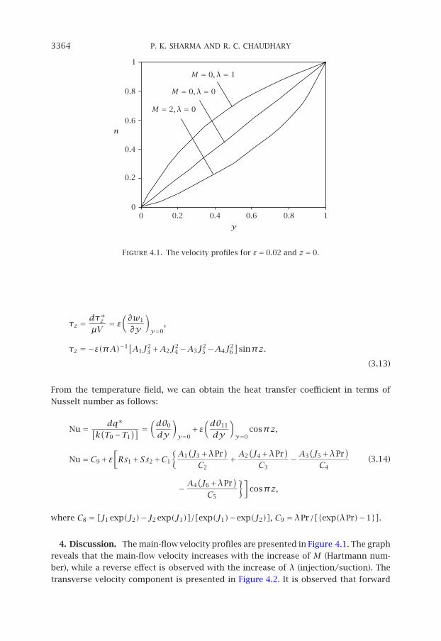
Figure 4.1. The velocity profiles for ε = 0.02 and z = 0.
τz = dτ∗z
µV= ε(∂w1
∂y
)y=0
,
τz =−ε(πA)−1[A1J23 +A2J2
4 −A3J25 −A4J2
6
]sinπz.
(3.13)
From the temperature field, we can obtain the heat transfer coefficient in terms of
Nusselt number as follows:
Nu= dq∗[k(T0−T1
)] =(dθ0
dy
)y=0
+ε(dθ11
dy
)y=0
cosπz,
Nu= C9+ε[Rs1+Ss2+C1
{A1(J3+λPr
)C2
+ A2(J4+λPr
)C3
− A3(J5+λPr
)C4
− A4(J6+λPr
)C5
}]cosπz,
(3.14)
where C8 = [J1 exp(J2)−J2 exp(J1)]/[exp(J1)−exp(J2)], C9 = λPr/[{exp(λPr)−1}].
4. Discussion. The main-flow velocity profiles are presented in Figure 4.1. The graph
reveals that the main-flow velocity increases with the increase of M (Hartmann num-
ber), while a reverse effect is observed with the increase of λ (injection/suction). The
transverse velocity component is presented in Figure 4.2. It is observed that forward

MAGNETOHYDRODYNAMICS EFFECT ON THREE-DIMENSIONAL VISCOUS . . . 3365
0.15
0.05
−0.05
−0.15
00.2 0.4 0.6 0.8
1w1
y
M = 0, λ = 0.5
M = 2, λ = 0.5
M = 2, λ = 0
Figure 4.2. The transverse velocity components for z = 0.5.
Table 4.1. The values of pressure (p1) for z = 0.
y λ= 0.2, M = 0 λ= 0.5, M = 0 λ= 0.5, M = 2
0 22.468 8.8780 8.9312
0.1 15.752 6.2182 6.3015
0.2 10.604 4.1773 4.2728
0.3 6.5114 2.5520 2.6355
0.4 3.0665 1.1807 1.2316
0.5 −0.0732 −0.0773 −0.0661
0.6 −3.2202 −1.3342 −1.3715
0.7 −6.6877 −2.7281 −2.7983
0.8 −10.820 −4.3934 −4.4752
0.9 −16.030 −6.4960 −6.5628
1.0 −22.835 −9.2450 −9.2758
flow is developed from y = 0 to about y = 0.5, and then, onwards, there is backward
flow. It is due to the fact that the dragging action of the faster layer exerted on the
fluid particles in the neighborhood of the stationary plate is sufficient to overcome the
adverse pressure gradient, and hence there is forward flow. The dragging action of the
faster layer exerted on the fluid particles will be reduced due to the periodic suction at
the upper plate, and hence this dragging action is insufficient to overcome the adverse
pressure gradient and there is backward flow. It is noted that this backward flow is
just the optical image of the forward flow. Further, it is evident from this figure that
3366 P. K. SHARMA AND R. C. CHAUDHARY
2.5
2
1.5
1
0.5
00 0.2 0.4 0.6 0.8 1
τx
λ
M = 2
M = 0
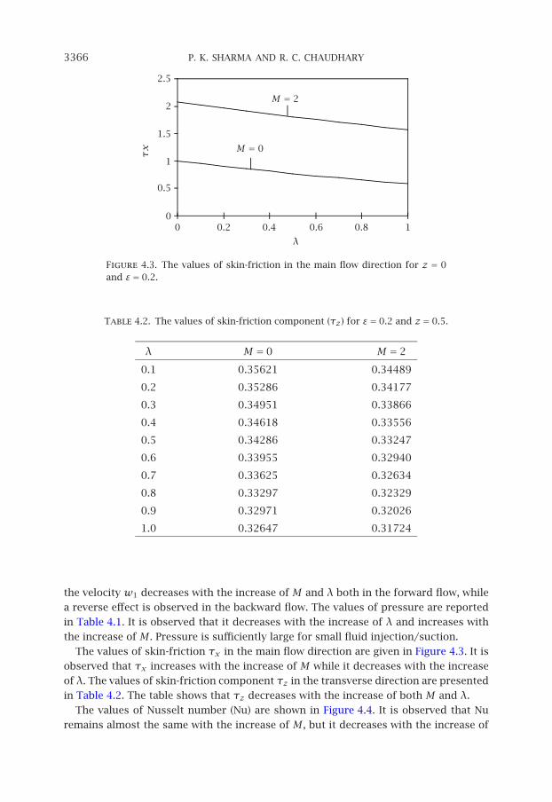
Figure 4.3. The values of skin-friction in the main flow direction for z = 0and ε = 0.2.
Table 4.2. The values of skin-friction component (τz) for ε = 0.2 and z = 0.5.
λ M = 0 M = 2
0.1 0.35621 0.34489
0.2 0.35286 0.34177
0.3 0.34951 0.33866
0.4 0.34618 0.33556
0.5 0.34286 0.33247
0.6 0.33955 0.32940
0.7 0.33625 0.32634
0.8 0.33297 0.32329
0.9 0.32971 0.32026
1.0 0.32647 0.31724
the velocity w1 decreases with the increase of M and λ both in the forward flow, while
a reverse effect is observed in the backward flow. The values of pressure are reported
in Table 4.1. It is observed that it decreases with the increase of λ and increases with
the increase of M . Pressure is sufficiently large for small fluid injection/suction.
The values of skin-friction τx in the main flow direction are given in Figure 4.3. It is
observed that τx increases with the increase of M while it decreases with the increase
of λ. The values of skin-friction component τz in the transverse direction are presented
in Table 4.2. The table shows that τz decreases with the increase of both M and λ.
The values of Nusselt number (Nu) are shown in Figure 4.4. It is observed that Nu
remains almost the same with the increase of M , but it decreases with the increase of

MAGNETOHYDRODYNAMICS EFFECT ON THREE-DIMENSIONAL VISCOUS . . . 3367
1
0.8
0.6
0.4
0.2
00 2 4 6 8 10
Nu
M
Pr = 0.71, λ = 0.2
Pr = 0.71, λ = 0.5
Pr = 7, λ = 0.2
Pr = 7, λ = 0.5
Figure 4.4. The values of Nusselt number for ε = 0.2 and z = 0.
λ in both situations (Pr = 0.71 (air) and Pr = 7 (water)). It is also clear from this figure
that Nu is much lower in the case of water (Pr= 7) than in the case of air (Pr= 0.71).
Acknowledgment. The authors are extremely thankful to the editor and the
anonymous reviewers for their valuable suggestions.
References
[1] H. A. Attia and N. A. Kotb, MHD flow between two parallel plates with heat transfer, ActaMech. 117 (1996), no. 1–4, 215–220.
[2] K. Gersten and J. F. Gross, Flow and heat transfer along a plane wall with periodic suction,Z. Angew. Math. Phys. 25 (1974), 399–408.
[3] H. P. Greenspan and G. F. Carrier, The magnetohydrodynamic flow past a flat plate, J. FluidMech. 6 (1959), 77–96.
[4] M. A. Hossain, S. K. Das, and I. Pop, Heat transfer response of MHD free convection flowalong a vertical plate to surface temperature oscillations, Internat. J. Non-LinearMech. 33 (1998), no. 3, 541–553.
[5] V. J. Rossow, On flow of electrically conducting fluids over a flat plate in the presence of atransverse magnetic field, Tech. Report 1358, NACA Ames Aeronautical Laboratory,1958.
[6] K. D. Singh, Hydromagnetic effects on the three-dimensional flow past a porous plate, Z.Angew. Math. Phys. 41 (1990), no. 3, 441–446.
[7] , Three-dimensional MHD oscillatory flow past a porous plate, ZAMM Z. Angew. Math.Mech. 71 (1991), no. 3, 192–195.
[8] , Three-dimensional viscous flow and heat transfer along a porous plate, ZAMM Z.Angew. Math. Mech. 73 (1993), no. 1, 58–61.
[9] , Three-dimensional Couette flow with transpiration cooling, Z. Angew. Math. Phys.50 (1999), no. 4, 661–668.
[10] P. Singh, V. P. Sharma, and U. N. Misra, Three dimensional fluctuating flow and heat transferalong a plate with suction, Int. J. Heat Mass Transfer 21 (1978), no. 8, 1117–1123.

3368 P. K. SHARMA AND R. C. CHAUDHARY
[11] , Three dimensional free convection flow and heat transfer along a porous verticalplate, Appl. Sci. Res. 34 (1978), no. 1, 105–115.
Pawan Kumar Sharma: Department of Mathematics, University of Rajasthan, Jaipur 302004,India
E-mail address: [email protected]
R. C. Chaudhary: Department of Mathematics, University of Rajasthan, Jaipur 302004, IndiaE-mail address: [email protected]

Submit your manuscripts athttp://www.hindawi.com
Hindawi Publishing Corporationhttp://www.hindawi.com Volume 2014
MathematicsJournal of
Hindawi Publishing Corporationhttp://www.hindawi.com Volume 2014
Mathematical Problems in Engineering
Hindawi Publishing Corporationhttp://www.hindawi.com
Differential EquationsInternational Journal of
Volume 2014
Applied MathematicsJournal of
Hindawi Publishing Corporationhttp://www.hindawi.com Volume 2014
Probability and StatisticsHindawi Publishing Corporationhttp://www.hindawi.com Volume 2014
Journal of
Hindawi Publishing Corporationhttp://www.hindawi.com Volume 2014
Mathematical PhysicsAdvances in
Complex AnalysisJournal of
Hindawi Publishing Corporationhttp://www.hindawi.com Volume 2014
OptimizationJournal of
Hindawi Publishing Corporationhttp://www.hindawi.com Volume 2014
CombinatoricsHindawi Publishing Corporationhttp://www.hindawi.com Volume 2014
International Journal of
Hindawi Publishing Corporationhttp://www.hindawi.com Volume 2014
Operations ResearchAdvances in
Journal of
Hindawi Publishing Corporationhttp://www.hindawi.com Volume 2014
Function Spaces
Abstract and Applied AnalysisHindawi Publishing Corporationhttp://www.hindawi.com Volume 2014
International Journal of Mathematics and Mathematical Sciences
Hindawi Publishing Corporationhttp://www.hindawi.com Volume 2014
The Scientific World JournalHindawi Publishing Corporation http://www.hindawi.com Volume 2014
Hindawi Publishing Corporationhttp://www.hindawi.com Volume 2014
Algebra
Discrete Dynamics in Nature and Society
Hindawi Publishing Corporationhttp://www.hindawi.com Volume 2014
Hindawi Publishing Corporationhttp://www.hindawi.com Volume 2014
Decision SciencesAdvances in
Discrete MathematicsJournal of
Hindawi Publishing Corporationhttp://www.hindawi.com
Volume 2014 Hindawi Publishing Corporationhttp://www.hindawi.com Volume 2014
Stochastic AnalysisInternational Journal of
Recommended