MAE 552 – Heuristic Optimization
Lecture 6
February 4, 2002
Summary of Traditional Methods
• We have learned up to this point that ‘traditional’ local search algorithms are not robust for a wide variety of problems.
• 3 main algorithms studied:
1. Hill-Climbing Method: Moves to the peak of a portion of the design space. Large tendency to get caught in local optima.
2. Enumerative Method: Only practical for small problems. Guaranteed to find the global optimal when properly applied.
3. Greedy Algorithms: Only a portion of the problem is considered at a time. Example: For NLP this consists of a series of line searches in n directions.
Summary of Traditional Methods
• When properly applied these methods can be very efficient.
• If you are faced with a quadratic problem, you should use a method like Newton’s.
• If you are faced with a linear problem, the most efficient method is simplex.
• It is important that the strengths and weaknesses of the algorithms is well understood.
• Most real-world problems cannot be successfully solved with traditional. If they could they would have been solved already.
• More powerful and robust methods are needed!!!!
Escaping Local Minima
• All of the methods discussed so far have either of the following characteristics.
1. They guarantee finding a global solution, but are too expensive, computationally speaking, practical problems.
2. They get stuck in local optima.
• There are two options,
(1) speed up algorithms that guarantee global optimality OR
(2) Design algorithms that are capable of escaping local optima.
Escaping Local Minima
• Can we speed up algorithms that guarantee global optimality? ----------------NO!!!
• Why? -------Because the problems that we are really interested in solving are NP-hard
AND• There are no polynomial time algorithms to solve
NP-hard problems• Even large, large orders of magnitude increases in
computer speed would not make a dent in most moderately sized problems.
Escaping Local Minima
• This leaves us with the option of designing algorithms that escape local minima. How?
1. Use the idea of the iterated hill climber, restart a local search algorithm multiple times and try to cover the search space.
2. Introduce parameters that allow the search to escape a local minima.
Simulated Annealing
• Simulated Annealing or SA is a global optimization technique that imitates the physical annealing process of a solid.
• SA is a robust approach that is extremely good for problems w/local minima.
• It typically can find a global optimum in a reasonable amount of CPU time.
• SA has been widely used for combinatorial functions with great success. It has been used less often for continuous problems with constraints although there is no reason it can’t.
Simulated Annealing
• SA can find better solutions that gradient-based methods on multi-modal, non-monotonic problems.
• It is more efficient than enumerative search methods as well which require enormous amounts of function evaluations.
• SA was derived from the ‘Metropolis Monte Carlo’ algorithm and was introduced by Kirkpatrick in
• It locates the near global optimal solutions by simulating the physical annealing process of a solid into its lowest energy state (ground state).
Simulated Annealing-Introduction
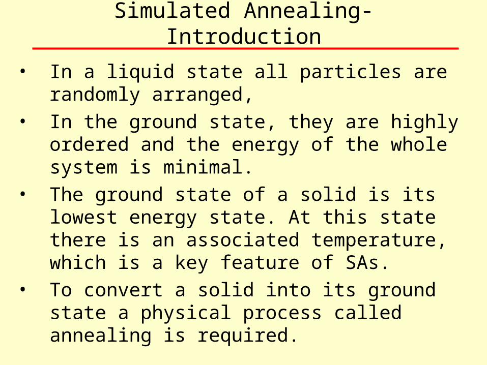
• In a liquid state all particles are randomly arranged, • In the ground state, they are highly ordered and the
energy of the whole system is minimal.• The ground state of a solid is its lowest energy state. At
this state there is an associated temperature, which is a key feature of SAs.
• To convert a solid into its ground state a physical process called annealing is required.
Simulated Annealing - Introduction
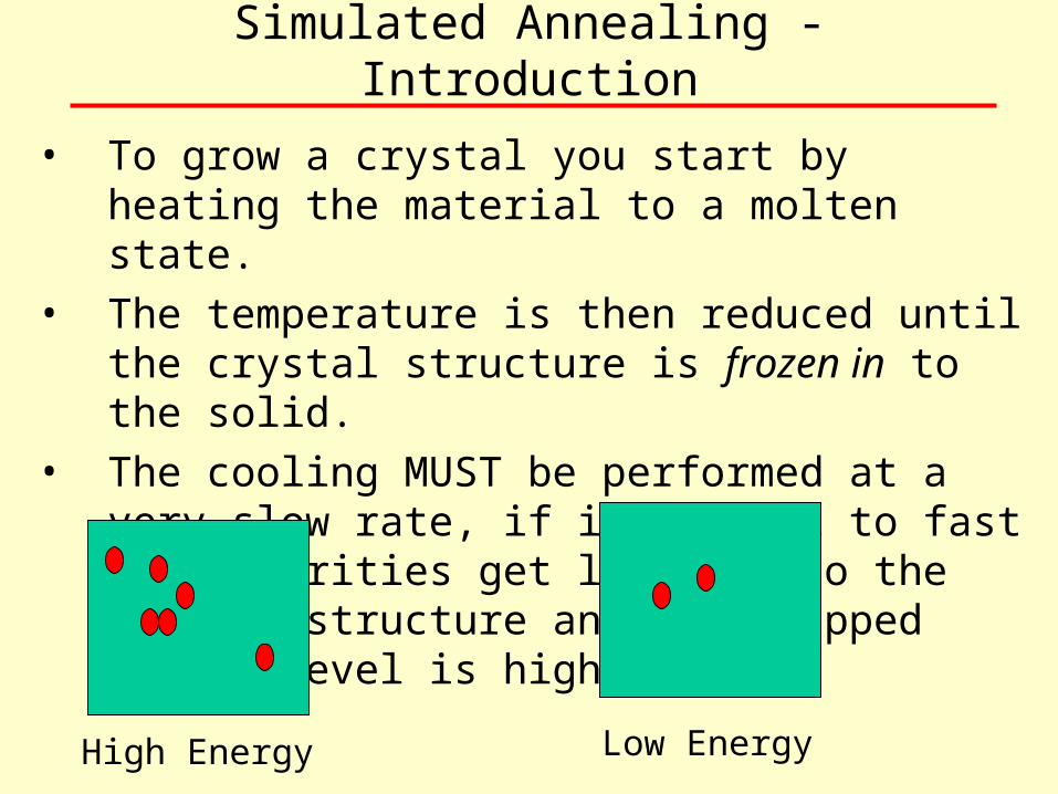
• To grow a crystal you start by heating the material to a molten state.
• The temperature is then reduced until the crystal structure is frozen in to the solid.
• The cooling MUST be performed at a very slow rate, if it is cool to fast irregularities get locked into the crystal structure and the trapped energy level is high.
High Energy Low Energy
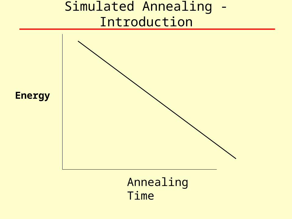
Simulated Annealing - Introduction
Energy
Annealing Time
Physical Annealing
• Annealing first melts a solid by increasing the temperature of the heat bath to a value at which all particles are randomly ordered.
• In this new state, where particles are randomly ordered, the solid has become a liquid. The temperature is then lowered sufficiently slowly so as to allow it to come to thermal equilibrium at each temperature.
• By this type of procedure the ground state is finally reached.
Physical Annealing
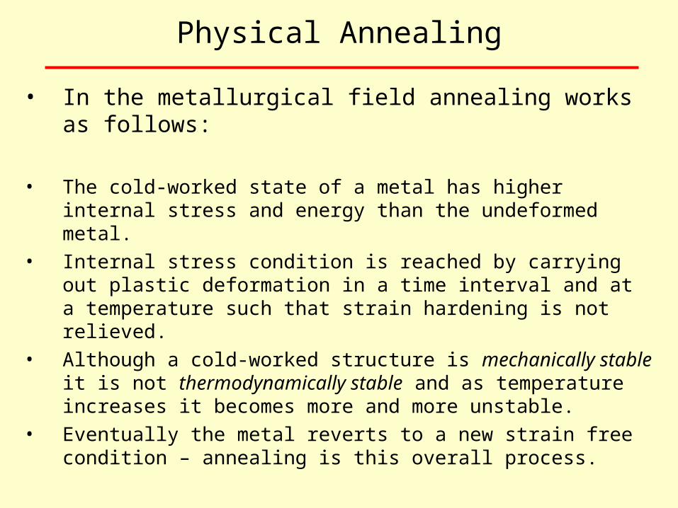
• In the metallurgical field annealing works as follows:
• The cold-worked state of a metal has higher internal stress and energy than the undeformed metal.
• Internal stress condition is reached by carrying out plastic deformation in a time interval and at a temperature such that strain hardening is not relieved.
• Although a cold-worked structure is mechanically stable it is not thermodynamically stable and as temperature increases it becomes more and more unstable.
• Eventually the metal reverts to a new strain free condition – annealing is this overall process.
Physical Annealing - Stages
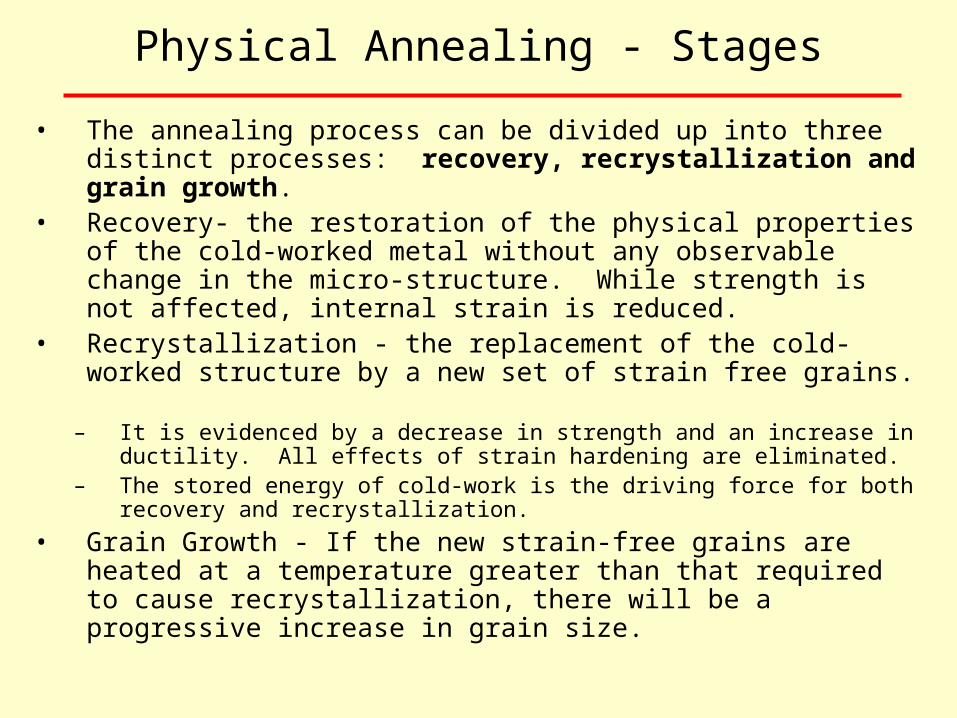
• The annealing process can be divided up into three distinct processes: recovery, recrystallization and grain growth.
• Recovery- the restoration of the physical properties of the cold-worked metal without any observable change in the micro-structure. While strength is not affected, internal strain is reduced.
• Recrystallization - the replacement of the cold-worked structure by a new set of strain free grains.
– It is evidenced by a decrease in strength and an increase in ductility. All effects of strain hardening are eliminated.
– The stored energy of cold-work is the driving force for both recovery and recrystallization.
• Grain Growth - If the new strain-free grains are heated at a temperature greater than that required to cause recrystallization, there will be a progressive increase in grain size.

Physical Annealing
Six main variables influence recrystallization:
1. Amount of prior deformation
2. Temp
3. Time
4. Initial Grain Size
5. Composition of Material
6. Amount of recovery prior to the start of recrystallization
Physical Annealing
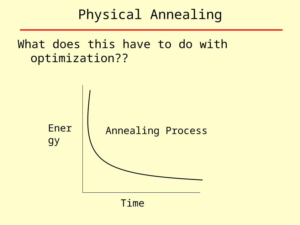
What does this have to do with optimization??
Energy
Time
Annealing Process
Physical Annealing
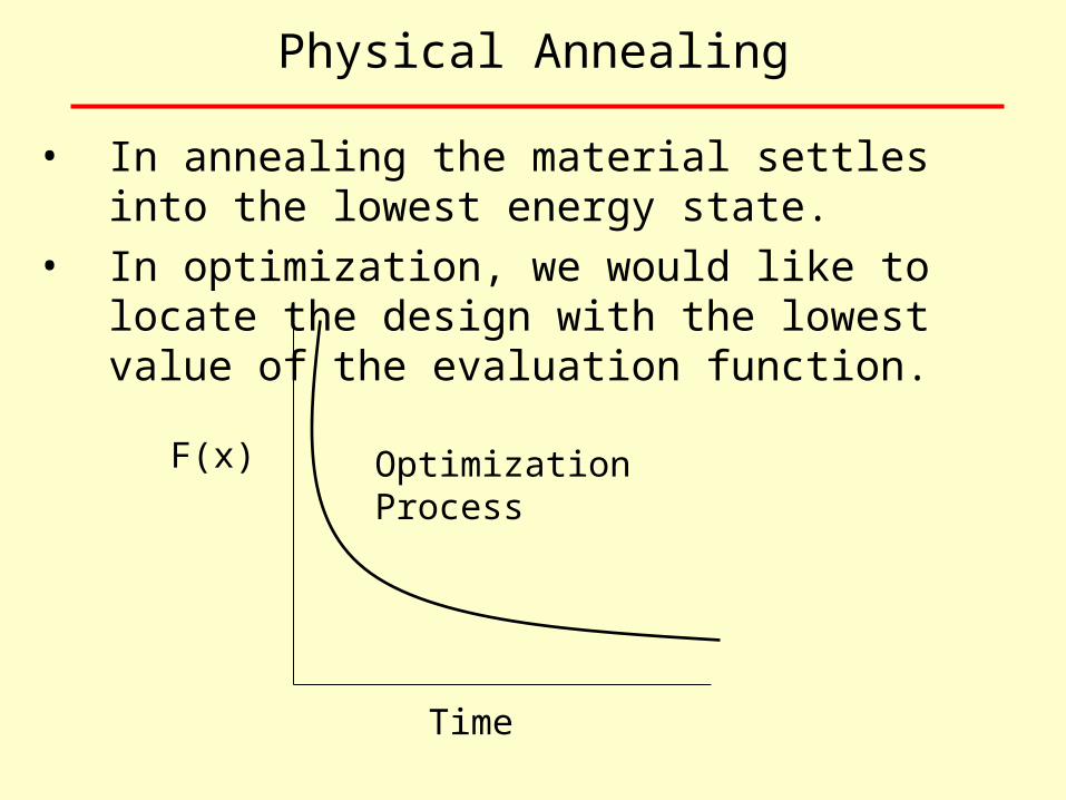
• In annealing the material settles into the lowest energy state.
• In optimization, we would like to locate the design with the lowest value of the evaluation function.
F(x)
Time
Optimization Process
Simulated Annealing
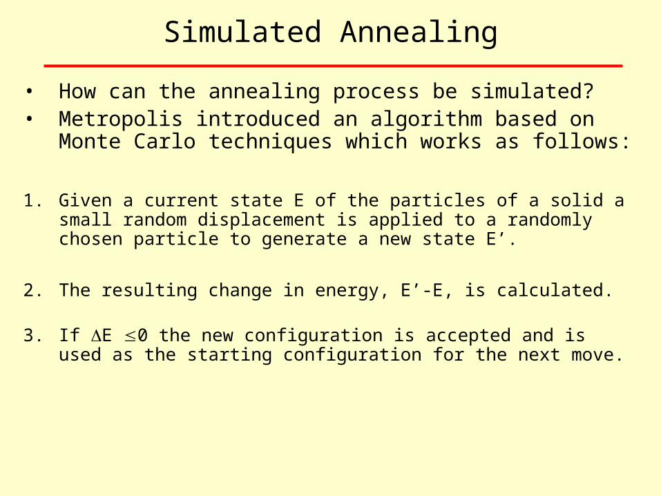
• How can the annealing process be simulated?• Metropolis introduced an algorithm based on Monte
Carlo techniques which works as follows:
1. Given a current state E of the particles of a solid a small random displacement is applied to a randomly chosen particle to generate a new state E’.
2. The resulting change in energy, E’-E, is calculated.
3. If E 0 the new configuration is accepted and is used as the starting configuration for the next move.
Simulated Annealing
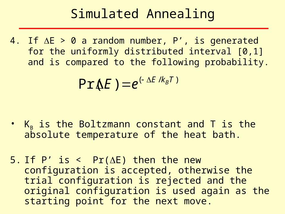
4. If E > 0 a random number, P’, is generated for the uniformly distributed interval [0,1] and is compared to the following probability.
)/()Pr( TkE BeE
• KB is the Boltzmann constant and T is the absolute temperature of the heat bath.
5. If P’ is < Pr(E) then the new configuration is accepted, otherwise the trial configuration is rejected and the original configuration is used again as the starting point for the next move.
Simulated Annealing
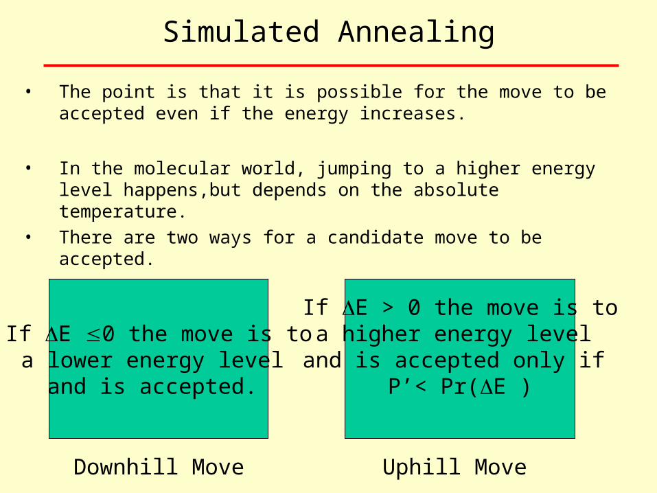
• The point is that it is possible for the move to be accepted even if the energy increases.
• In the molecular world, jumping to a higher energy level happens,but depends on the absolute temperature.
• There are two ways for a candidate move to be accepted.
Downhill Move Uphill Move
If E 0 the move is toa lower energy level
and is accepted.
If E > 0 the move is toa higher energy level
and is accepted only if P’< Pr(E )
Simulated Annealing
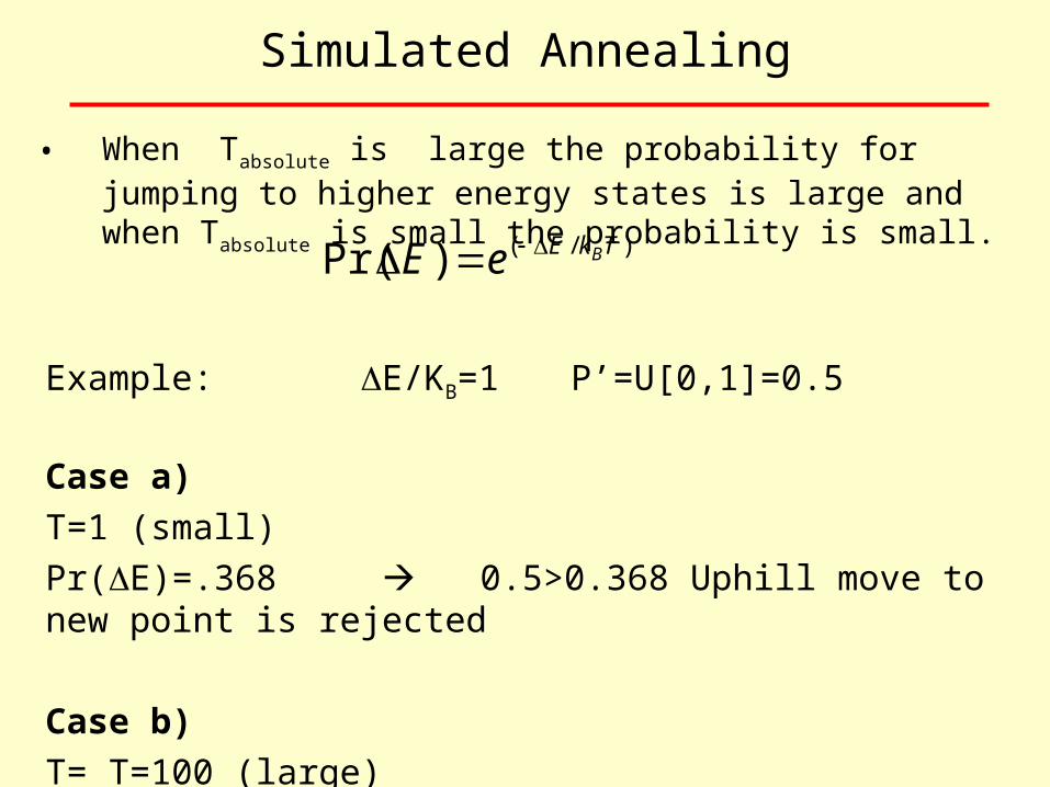
• When Tabsolute is large the probability for jumping to higher energy states is large and when Tabsolute is small the probability is small. )/()Pr( TkE BeE
Example: E/KB=1 P’=U[0,1]=0.5
Case a)
T=1 (small)
Pr(E)=.368 0.5>0.368 Uphill move to new point is rejected
Case b)
T= T=100 (large)
Pr(E)=.99 0.5<0.99 Uphill move to new point is accepted
If we had gotten a random number # of .5 and T=1 P’=.5 is not less that .368 so the move is
rejected but P’ < .99 so this move is accepted.
Simulated Annealing
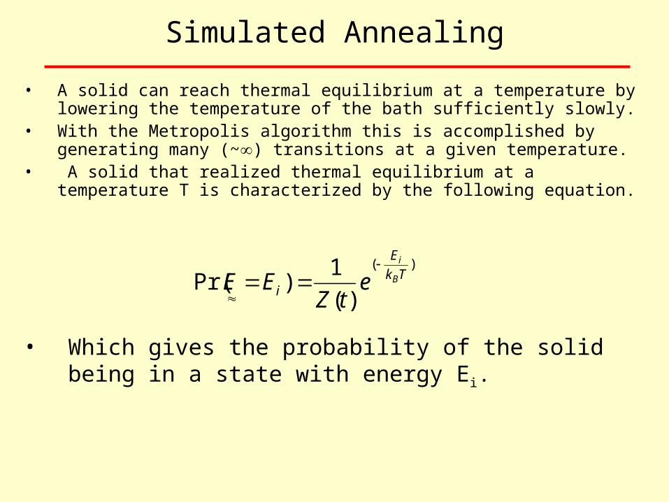
• A solid can reach thermal equilibrium at a temperature by lowering the temperature of the bath sufficiently slowly.
• With the Metropolis algorithm this is accomplished by generating many (~) transitions at a given temperature.
• A solid that realized thermal equilibrium at a temperature T is characterized by the following equation.
)(
)(
1)Pr( Tk
E
iB
i
etZ
EE
• Which gives the probability of the solid being in a state with energy Ei.
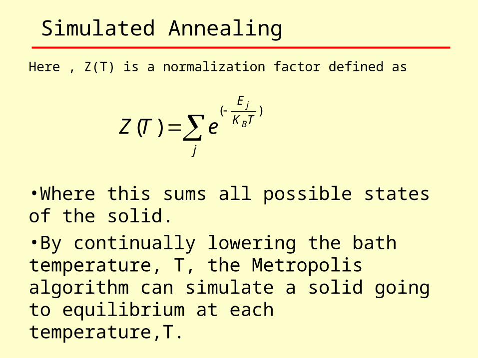
Here , Z(T) is a normalization factor defined as
j
TK
E
B
j
eTZ)(
)(
Simulated Annealing
•Where this sums all possible states of the solid. •By continually lowering the bath temperature, T, the Metropolis algorithm can simulate a solid going to equilibrium at each temperature,T.
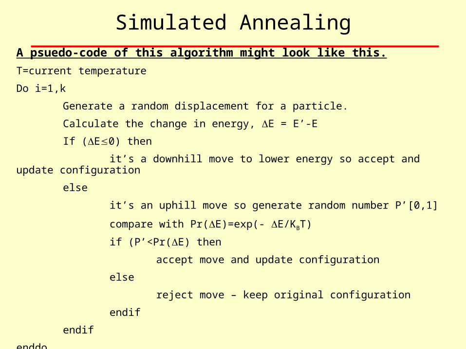
Simulated AnnealingA psuedo-code of this algorithm might look like this.
T=current temperature
Do i=1,k
Generate a random displacement for a particle.
Calculate the change in energy, E = E’-E
If (E0) then
it’s a downhill move to lower energy so accept and update configuration
else
it’s an uphill move so generate random number P’[0,1]
compare with Pr(E)=exp(- E/KBT)
if (P’<Pr(E) then
accept move and update configuration
else
reject move – keep original configuration
endif
endif
enddo
Recommended


![Informed [Heuristic] Search - University of Delawaredecker/courses/681s07/pdfs/04-Heuristic...Informed [Heuristic] Search Heuristic: “A rule of thumb, simplification, or educated](https://img.pdfslide.us/doc/110x75/5aa1e13c7f8b9a84398c48b6/informed-heuristic-search-university-of-delaware-deckercourses681s07pdfs04-heuristicinformed.jpg)