macroeconomics fifth edition
N. Gregory Mankiw
PowerPoint® Slides by Ron Cronovichm
acro
© 2004 Worth Publishers, all rights reserved
CHAPTER THIRTEEN
Aggregate Supply
Edited by:Taggert J. BrooksUW-La Crosse
CHAPTER 13CHAPTER 13 Aggregate Supply Aggregate Supply slide 2
Learning objectivesLearning objectives
three models of aggregate supply in which output depends positively on the price level in the short run
the short-run tradeoff between inflation and unemployment known as the Phillips curve
CHAPTER 13CHAPTER 13 Aggregate Supply Aggregate Supply slide 3
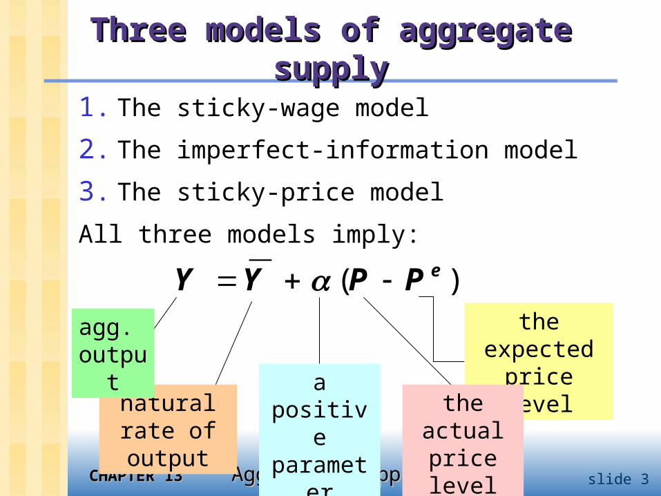
Three models of aggregate supplyThree models of aggregate supply
1. The sticky-wage model
2. The imperfect-information model
3. The sticky-price model
All three models imply:
( )eY Y P P
natural rate of output
a positive paramet
er
the expected price level
the actual price level
agg. outpu
t
CHAPTER 13CHAPTER 13 Aggregate Supply Aggregate Supply slide 4
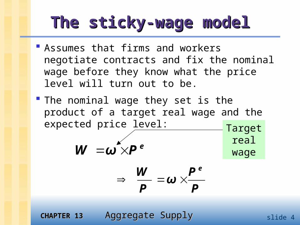
The sticky-wage modelThe sticky-wage model
Assumes that firms and workers negotiate contracts and fix the nominal wage before they know what the price level will turn out to be.
The nominal wage they set is the product of a target real wage and the expected price level:
eW ω P eW P
ωP P
Target real
wage
CHAPTER 13CHAPTER 13 Aggregate Supply Aggregate Supply slide 5
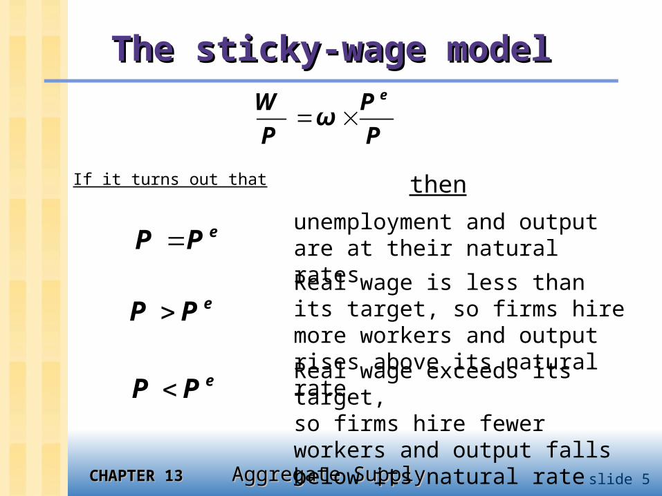
The sticky-wage modelThe sticky-wage model
If it turns out that
eW Pω
P P
eP P
eP P
eP P
then
unemployment and output are at their natural rates
Real wage is less than its target, so firms hire more workers and output rises above its natural rateReal wage exceeds its target,
so firms hire fewer workers and output falls below its natural rate
CHAPTER 13CHAPTER 13 Aggregate Supply Aggregate Supply slide 7
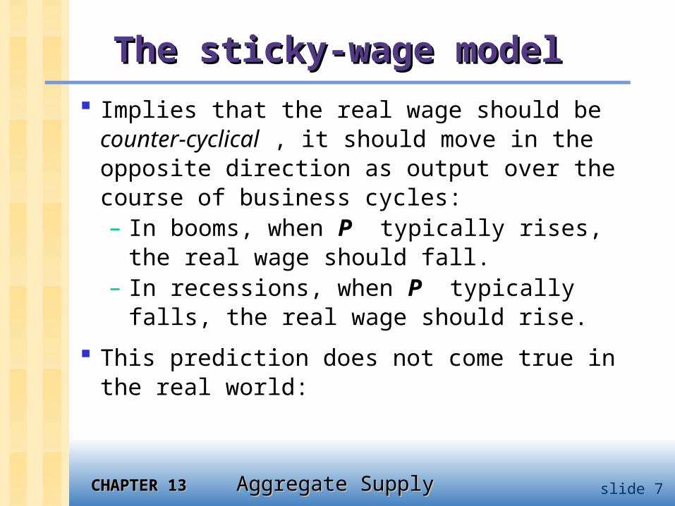
The sticky-wage modelThe sticky-wage model
Implies that the real wage should be counter-cyclical , it should move in the opposite direction as output over the course of business cycles:– In booms, when P typically rises, the
real wage should fall. – In recessions, when P typically falls,
the real wage should rise.
This prediction does not come true in the real world:

CHAPTER 13CHAPTER 13 Aggregate Supply Aggregate Supply slide 8
The cyclical behavior of the real wageThe cyclical behavior of the real wageP
erc
en
tag
e
ch
an
ge
in r
eal w
ag
e
Percentage change in real GDP
1982
1975
19931992
1960
1996
19991997
1998
1979
1970
1980
1991
1974
1990
19842000
1972
1965
-3 -2 -1 0 1 2 3 7 8654
4
3
2
1
0
-1
-2
-3
-4
-5
CHAPTER 13CHAPTER 13 Aggregate Supply Aggregate Supply slide 9
The imperfect-information modelThe imperfect-information model
Assumptions:
all wages and prices perfectly flexible, all markets clear
each supplier produces one good, consumes many goods
each supplier knows the nominal price of the good she produces, but does not know the overall price level
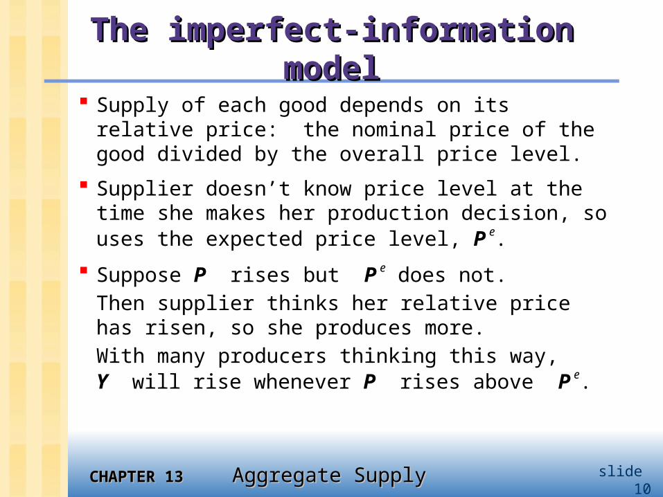
CHAPTER 13CHAPTER 13 Aggregate Supply Aggregate Supply slide 10
The imperfect-information modelThe imperfect-information model
Supply of each good depends on its relative price: the nominal price of the good divided by the overall price level.
Supplier doesn’t know price level at the time she makes her production decision, so uses the expected price level, P
e.
Suppose P rises but P e does not.
Then supplier thinks her relative price has risen, so she produces more. With many producers thinking this way, Y will rise whenever P rises above P
e.
CHAPTER 13CHAPTER 13 Aggregate Supply Aggregate Supply slide 11
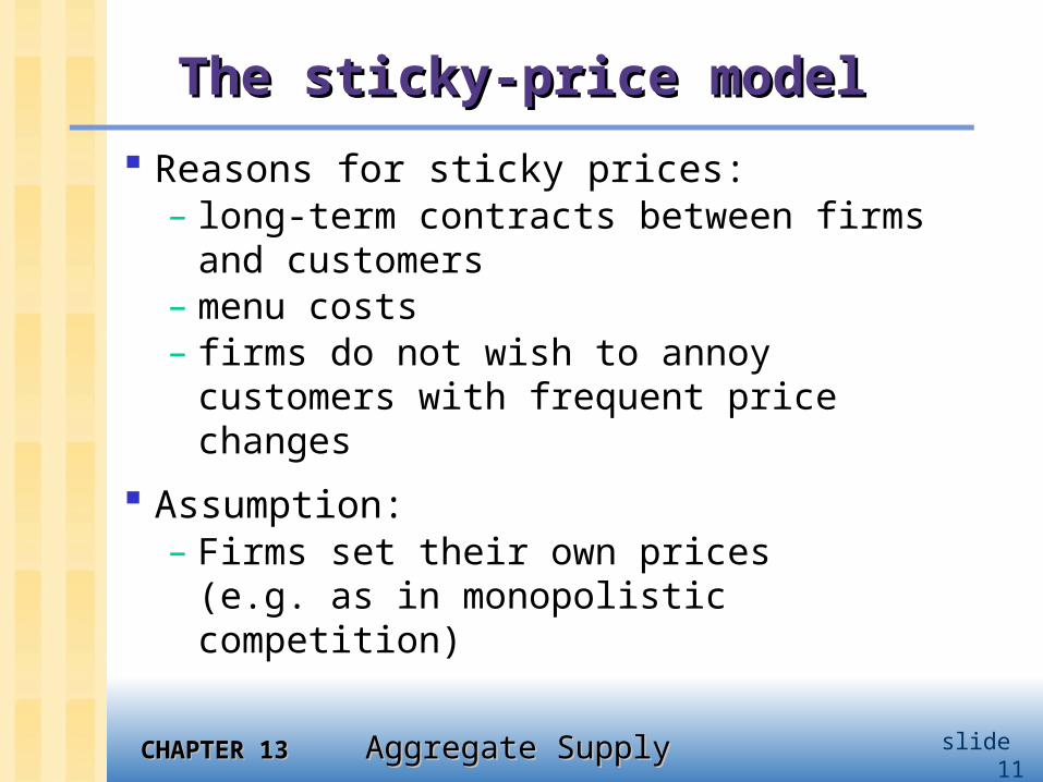
The sticky-price modelThe sticky-price model
Reasons for sticky prices:– long-term contracts between firms
and customers– menu costs– firms do not wish to annoy customers
with frequent price changes
Assumption:– Firms set their own prices
(e.g. as in monopolistic competition)
CHAPTER 13CHAPTER 13 Aggregate Supply Aggregate Supply slide 12
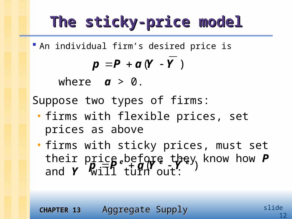
The sticky-price modelThe sticky-price model
An individual firm’s desired price is
where a > 0.
Suppose two types of firms:• firms with flexible prices, set prices as
above• firms with sticky prices, must set their
price before they know how P and Y will turn out:
( )p P Y Y a
( )e e ep P Y Y a
CHAPTER 13CHAPTER 13 Aggregate Supply Aggregate Supply slide 13
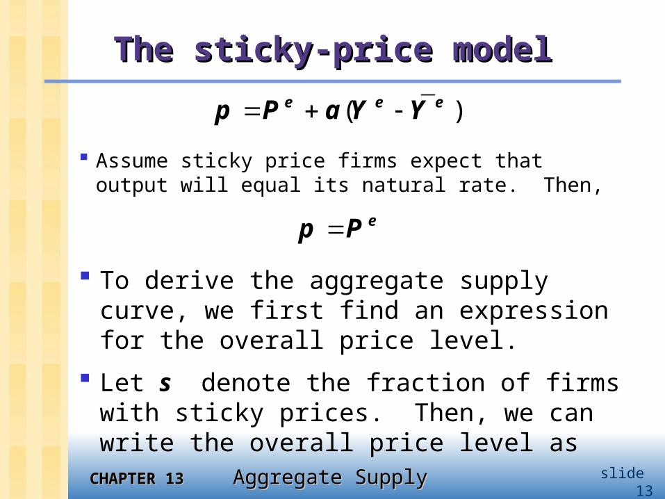
The sticky-price modelThe sticky-price model
Assume sticky price firms expect that output will equal its natural rate. Then,
( )e e ep P Y Y a
ep P
To derive the aggregate supply curve, we first find an expression for the overall price level.
Let s denote the fraction of firms with sticky prices. Then, we can write the overall price level as
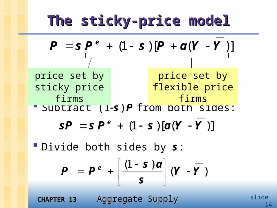
CHAPTER 13CHAPTER 13 Aggregate Supply Aggregate Supply slide 14
The sticky-price modelThe sticky-price model
Subtract (1s )P from both sides:
(1 )[ ( )]eP s P s P Y Y a
price set by flexible price
firms
price set by sticky price
firms
(1 )[ ( )]esP s P s Y Y a
Divide both sides by s :
(1 )( )e s
P P Y Ys
a
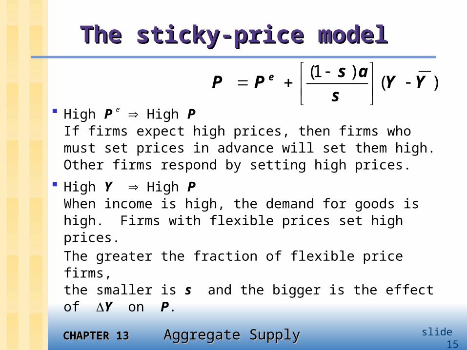
CHAPTER 13CHAPTER 13 Aggregate Supply Aggregate Supply slide 15
The sticky-price modelThe sticky-price model
High P e High PIf firms expect high prices, then firms who must set prices in advance will set them high.Other firms respond by setting high prices.
High Y High P When income is high, the demand for goods is high. Firms with flexible prices set high prices. The greater the fraction of flexible price firms, the smaller is s and the bigger is the effect of Y on P.
(1 )( )e s
P P Y Ys
a
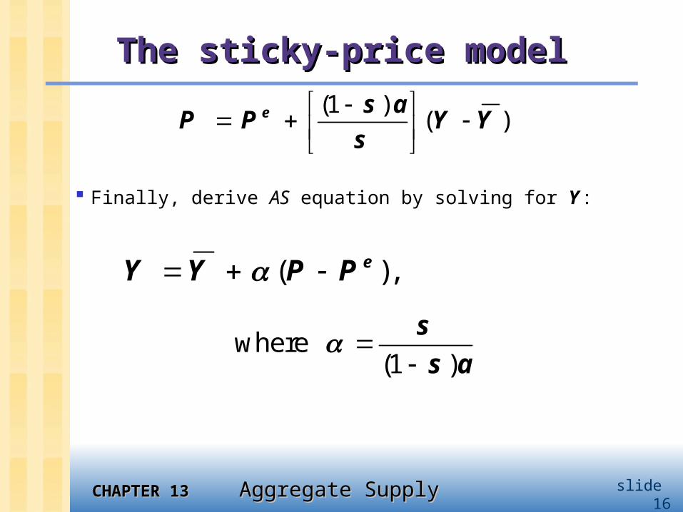
CHAPTER 13CHAPTER 13 Aggregate Supply Aggregate Supply slide 16
The sticky-price modelThe sticky-price model
Finally, derive AS equation by solving for Y :
(1 )( )e s
P P Y Ys
a
( ),eY Y P P
where (1 )
ss
a
CHAPTER 13CHAPTER 13 Aggregate Supply Aggregate Supply slide 17
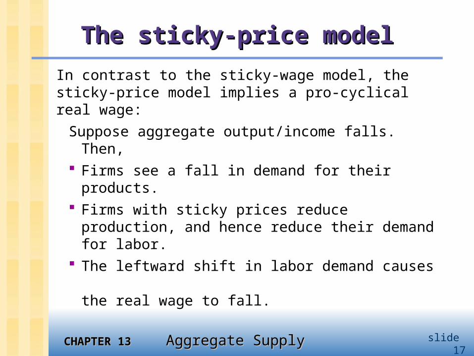
The sticky-price modelThe sticky-price model
In contrast to the sticky-wage model, the sticky-price model implies a pro-cyclical real wage:
Suppose aggregate output/income falls. Then,
Firms see a fall in demand for their products.
Firms with sticky prices reduce production, and hence reduce their demand for labor.
The leftward shift in labor demand causes the real wage to fall.
CHAPTER 13CHAPTER 13 Aggregate Supply Aggregate Supply slide 18
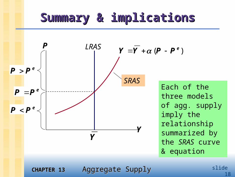
Summary & implicationsSummary & implications
Each of the three models of agg. supply imply the relationship summarized by the SRAS curve & equation
Y
P LRAS
Y
SRAS
( )eY Y P P
eP P
eP P
eP P
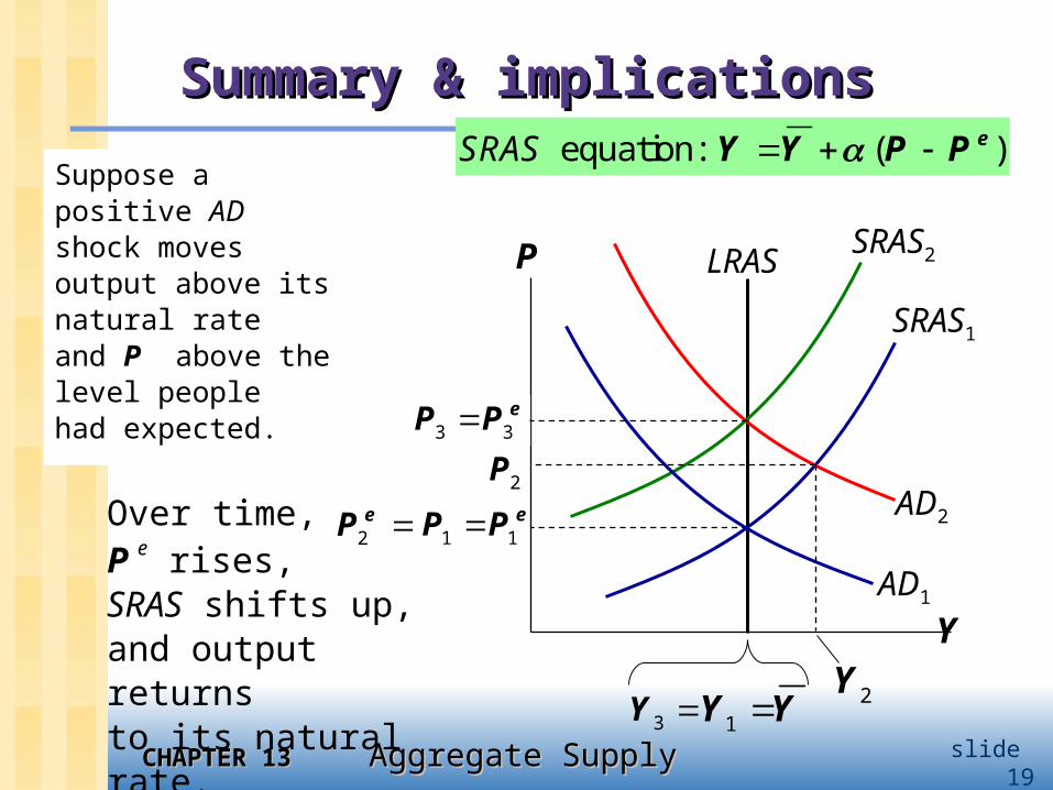
CHAPTER 13CHAPTER 13 Aggregate Supply Aggregate Supply slide 19
Summary & implicationsSummary & implications
Suppose a positive AD shock moves output above its natural rate and P above the level people had expected.
Y
P LRAS
SRAS1
equation: ( )eY Y P P SRAS
1 1eP P
SRAS2
AD1
AD22eP
2P3 3
eP P
Over time, P e rises, SRAS shifts up,and output returns to its natural rate. 1Y Y 2Y
3Y
CHAPTER 13CHAPTER 13 Aggregate Supply Aggregate Supply slide 20
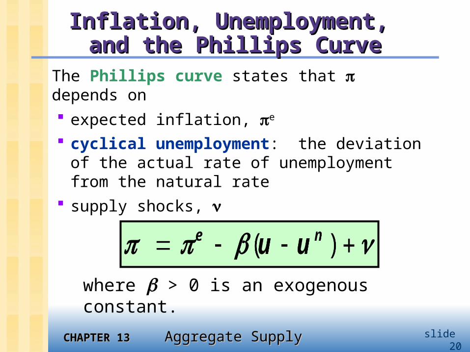
Inflation, Unemployment, Inflation, Unemployment, and the Phillips Curveand the Phillips Curve
The Phillips curve states that depends on expected inflation, e
cyclical unemployment: the deviation of the actual rate of unemployment from the natural rate
supply shocks,
where > 0 is an exogenous constant.
CHAPTER 13CHAPTER 13 Aggregate Supply Aggregate Supply slide 21
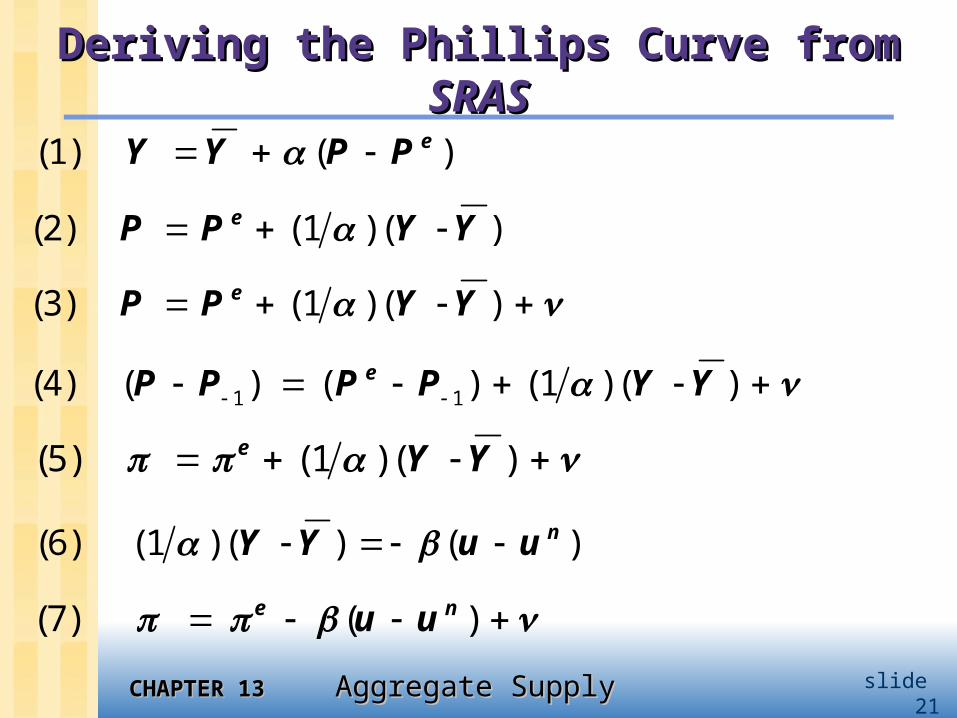
Deriving the Phillips Curve from Deriving the Phillips Curve from SRASSRAS
(1) ( )eY Y P P
(2) (1 )( )eP P Y Y
1 1(4) ( ) ( ) (1 )( )eP P P P Y Y
(5) (1 )( )e Y Y
(6) (1 )( ) ( )nY Y u u
(7) ( )e nu u
(3) (1 )( )eP P Y Y
CHAPTER 13CHAPTER 13 Aggregate Supply Aggregate Supply slide 22
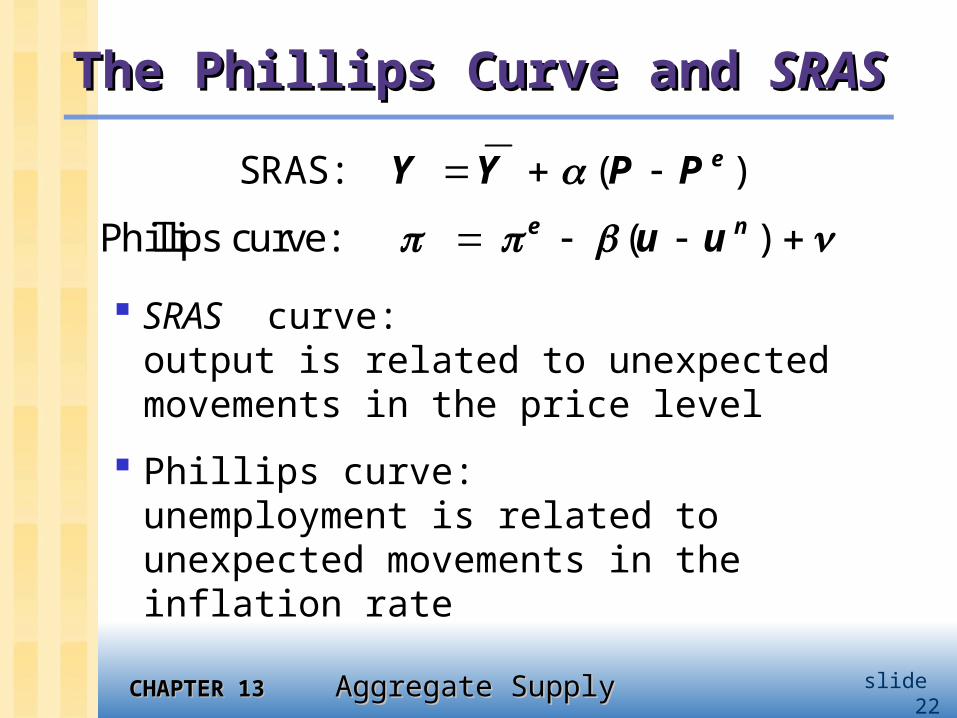
The Phillips Curve and The Phillips Curve and SRASSRAS
SRAS curve: output is related to unexpected movements in the price level
Phillips curve: unemployment is related to unexpected movements in the inflation rate
SRAS: ( )eY Y P P
Phillips curve: ( )e nu u
CHAPTER 13CHAPTER 13 Aggregate Supply Aggregate Supply slide 23
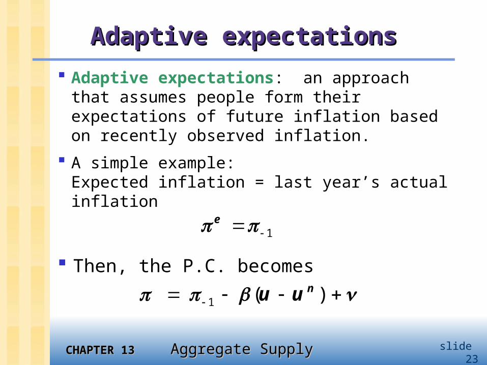
Adaptive expectationsAdaptive expectations
Adaptive expectations: an approach that assumes people form their expectations of future inflation based on recently observed inflation.
A simple example: Expected inflation = last year’s actual inflation
1 ( )nu u
1e
Then, the P.C. becomes
CHAPTER 13CHAPTER 13 Aggregate Supply Aggregate Supply slide 24
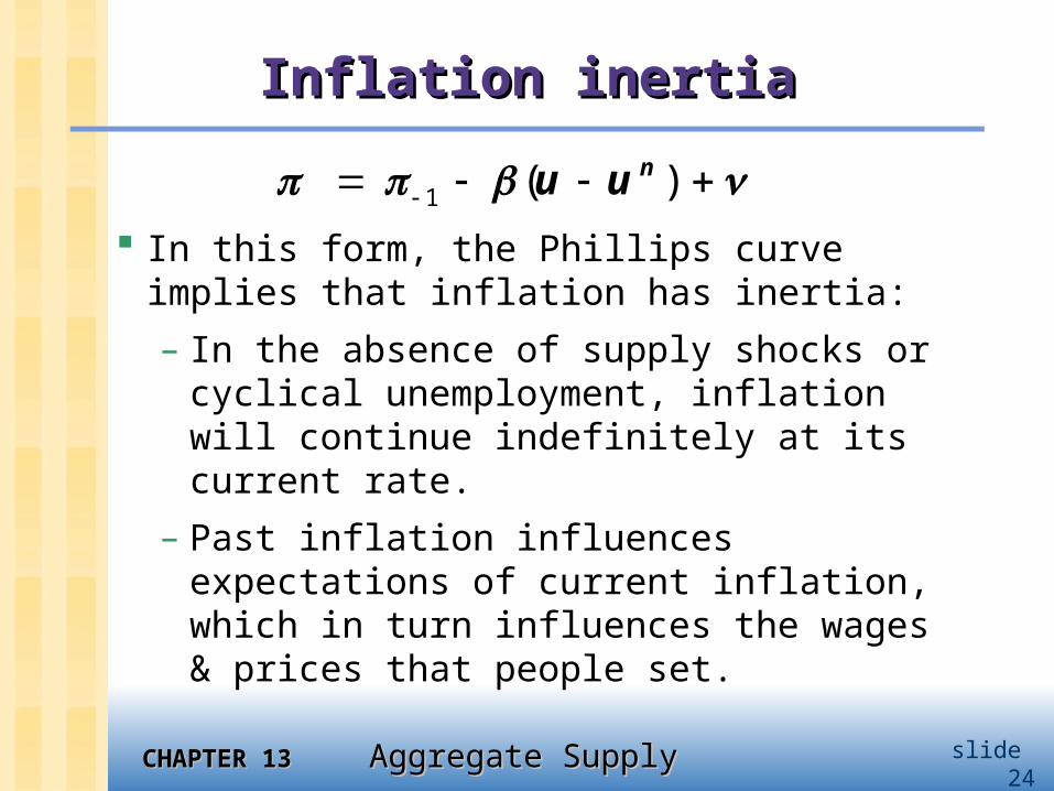
Inflation inertiaInflation inertia
In this form, the Phillips curve implies that inflation has inertia:
– In the absence of supply shocks or cyclical unemployment, inflation will continue indefinitely at its current rate.
– Past inflation influences expectations of current inflation, which in turn influences the wages & prices that people set.
1 ( )nu u
CHAPTER 13CHAPTER 13 Aggregate Supply Aggregate Supply slide 25
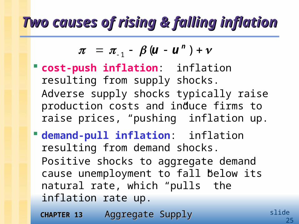
Two causes of rising & falling inflationTwo causes of rising & falling inflation
cost-push inflation: inflation resulting from supply shocks.Adverse supply shocks typically raise production costs and induce firms to raise prices, “pushing” inflation up.
demand-pull inflation: inflation resulting from demand shocks.Positive shocks to aggregate demand cause unemployment to fall below its natural rate, which “pulls” the inflation rate up.
1 ( )nu u
CHAPTER 13CHAPTER 13 Aggregate Supply Aggregate Supply slide 26
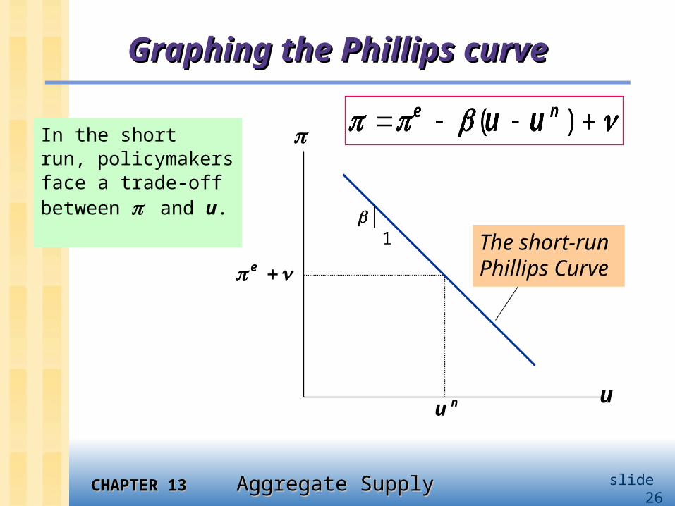
Graphing the Phillips curveGraphing the Phillips curve
In the short run, policymakers face a trade-off between and u.
u
nu
1
The short-run Phillips Curve
e
CHAPTER 13CHAPTER 13 Aggregate Supply Aggregate Supply slide 27
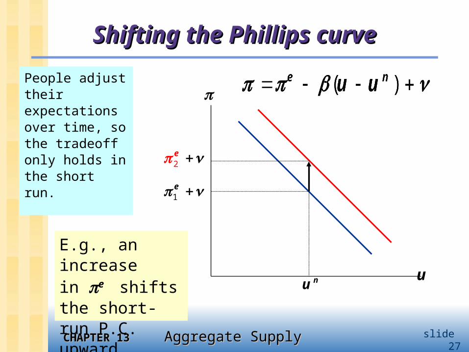
Shifting the Phillips curveShifting the Phillips curve
People adjust their expectations over time, so the tradeoff only holds in the short run.
u
nu
1e
2e
E.g., an increase in e shifts the short-run P.C. upward.
CHAPTER 13CHAPTER 13 Aggregate Supply Aggregate Supply slide 28
The sacrifice ratioThe sacrifice ratio
To reduce inflation, policymakers can contract agg. demand, causing unemployment to rise above the natural rate.
The sacrifice ratio measures the percentage of a year’s real GDP that must be foregone to reduce inflation by 1 percentage point.
Estimates vary, but a typical one is 5.
CHAPTER 13CHAPTER 13 Aggregate Supply Aggregate Supply slide 29
The sacrifice ratioThe sacrifice ratio Suppose policymakers wish to reduce
inflation from 6 to 2 percent. If the sacrifice ratio is 5, then reducing inflation by 4 points requires a loss of 45 = 20 percent of one year’s GDP.
This could be achieved several ways, e.g.– reduce GDP by 20% for one year– reduce GDP by 10% for each of two years– reduce GDP by 5% for each of four years
The cost of disinflation is lost GDP. One could use Okun’s law to translate this cost into unemployment.
CHAPTER 13CHAPTER 13 Aggregate Supply Aggregate Supply slide 30
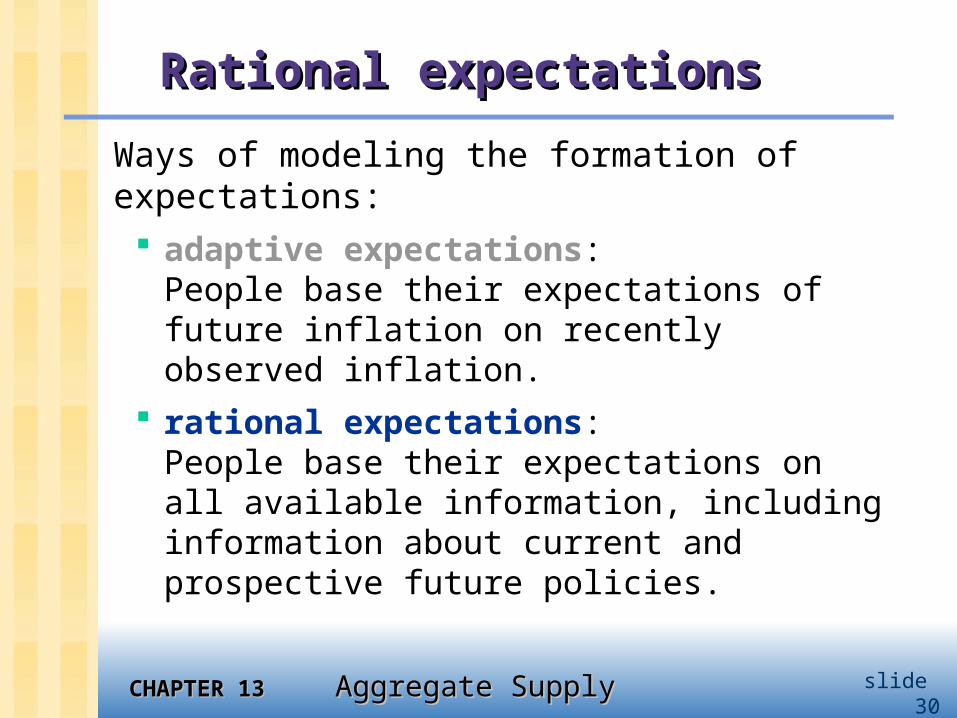
Rational expectations Rational expectations
Ways of modeling the formation of expectations: adaptive expectations:
People base their expectations of future inflation on recently observed inflation.
rational expectations:People base their expectations on all available information, including information about current and prospective future policies.
CHAPTER 13CHAPTER 13 Aggregate Supply Aggregate Supply slide 31
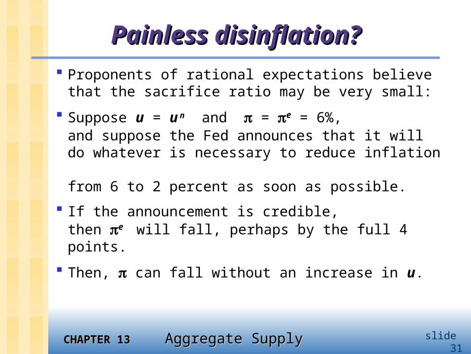
Painless disinflation?Painless disinflation?
Proponents of rational expectations believe that the sacrifice ratio may be very small:
Suppose u = u n and = e = 6%,
and suppose the Fed announces that it will do whatever is necessary to reduce inflation from 6 to 2 percent as soon as possible.
If the announcement is credible, then e will fall, perhaps by the full 4 points.
Then, can fall without an increase in u.
CHAPTER 13CHAPTER 13 Aggregate Supply Aggregate Supply slide 32
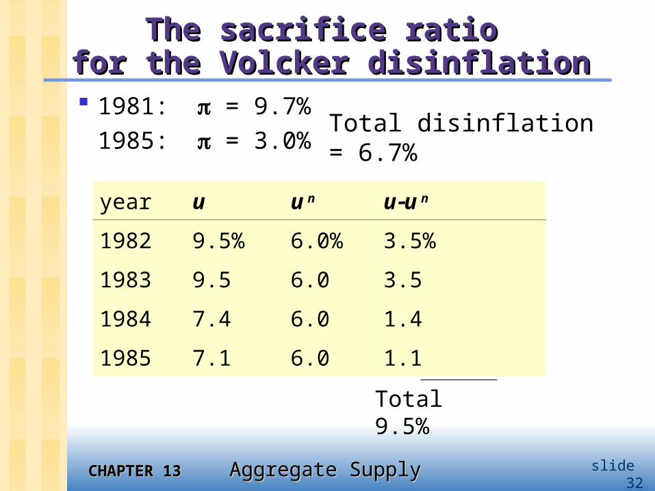
The sacrifice ratio The sacrifice ratio for the Volcker disinflationfor the Volcker disinflation
1981: = 9.7%1985: = 3.0%
year u u n uu n
1982 9.5% 6.0% 3.5%
1983 9.5 6.0 3.5
1984 7.4 6.0 1.4
1985 7.1 6.0 1.1
Total 9.5%
Total disinflation = 6.7%
CHAPTER 13CHAPTER 13 Aggregate Supply Aggregate Supply slide 33
The sacrifice ratio The sacrifice ratio for the Volcker disinflationfor the Volcker disinflation
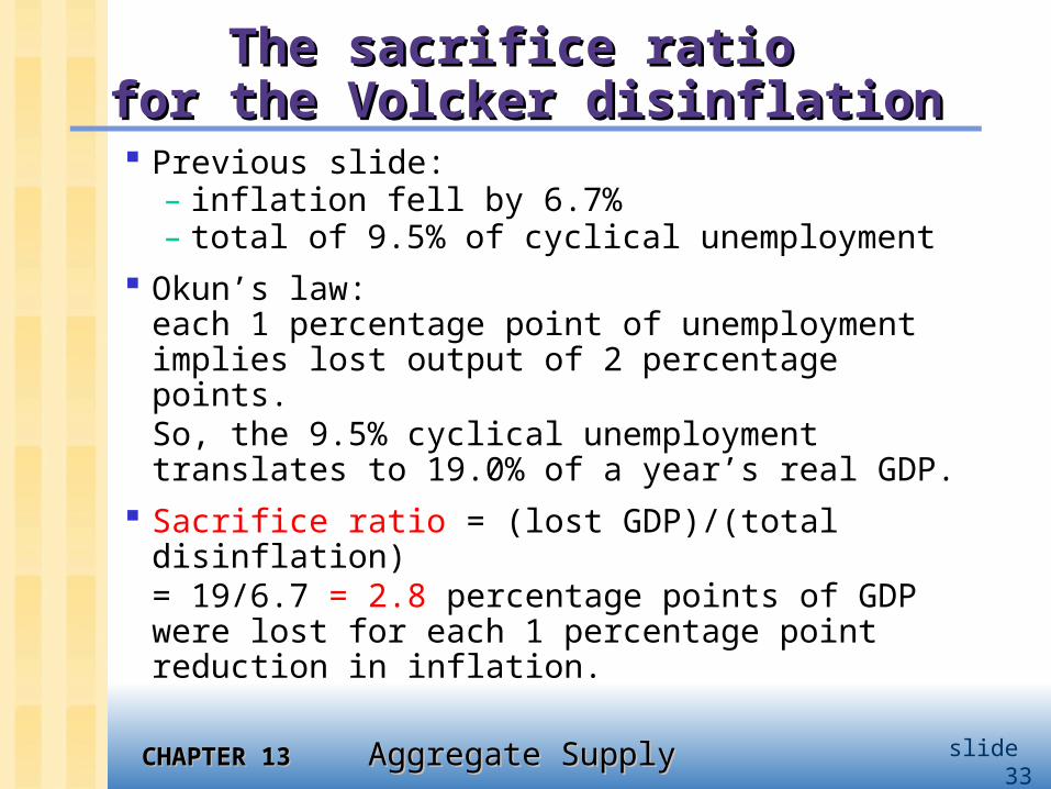
Previous slide:– inflation fell by 6.7%– total of 9.5% of cyclical unemployment
Okun’s law: each 1 percentage point of unemployment implies lost output of 2 percentage points. So, the 9.5% cyclical unemployment translates to 19.0% of a year’s real GDP.
Sacrifice ratio = (lost GDP)/(total disinflation)= 19/6.7 = 2.8 percentage points of GDP were lost for each 1 percentage point reduction in inflation.
CHAPTER 13CHAPTER 13 Aggregate Supply Aggregate Supply slide 34
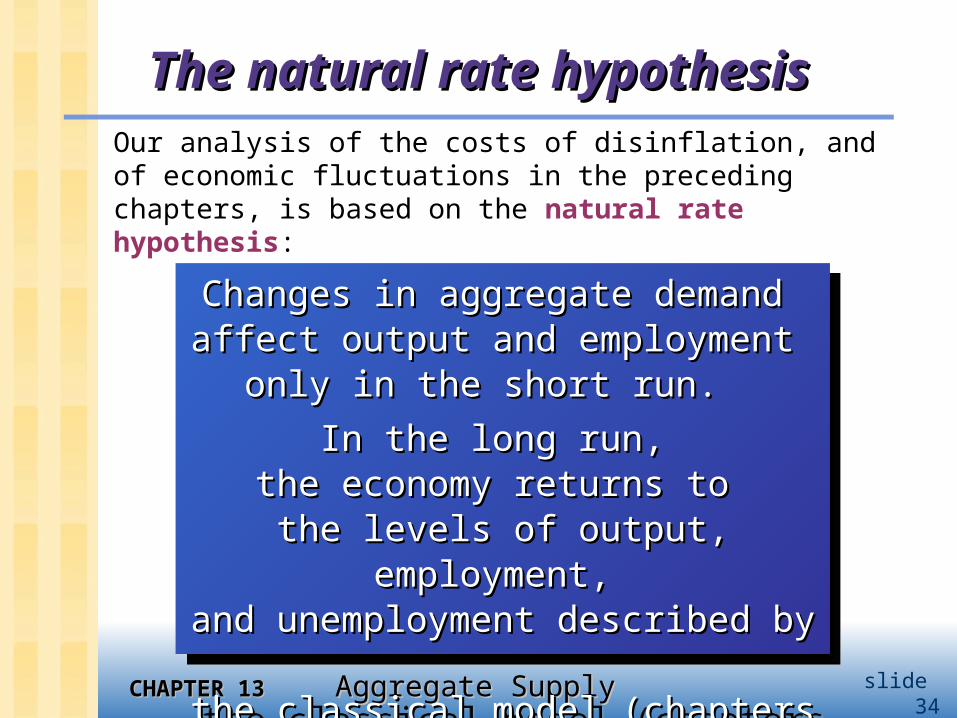
The natural rate hypothesisThe natural rate hypothesisOur analysis of the costs of disinflation, and of economic fluctuations in the preceding chapters, is based on the natural rate hypothesis:
Changes in aggregate demand Changes in aggregate demand affect output and employment affect output and employment
only in the short run. only in the short run.
In the long run, In the long run, the economy returns to the economy returns to
the levels of output, employment, the levels of output, employment, and unemployment described by and unemployment described by the classical model (chapters 3-8).the classical model (chapters 3-8).
CHAPTER 13CHAPTER 13 Aggregate Supply Aggregate Supply slide 35
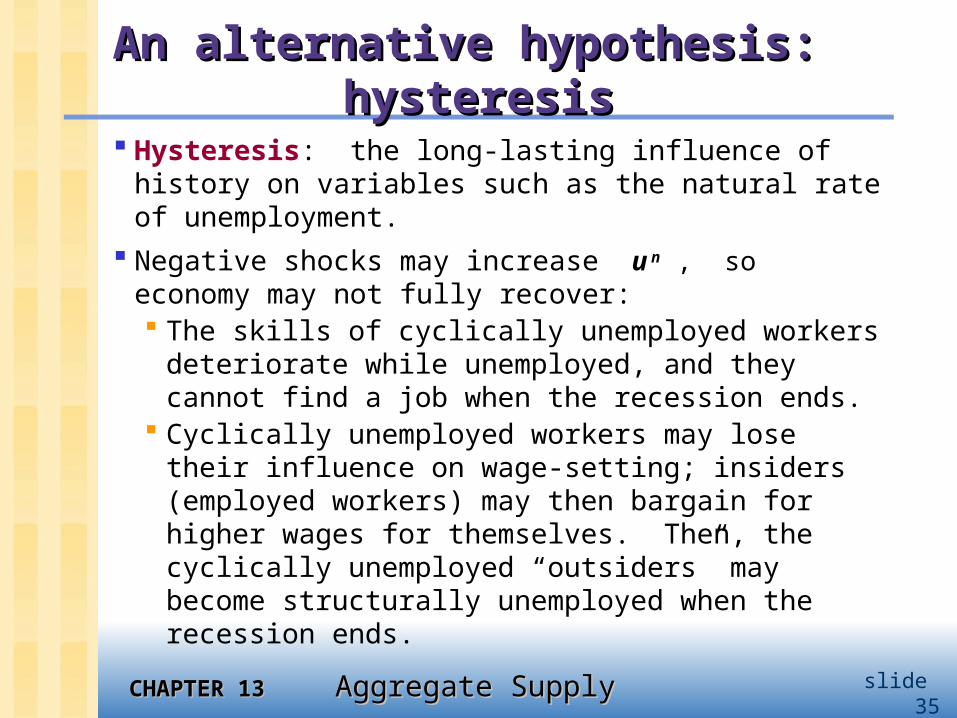
An alternative hypothesis: hysteresisAn alternative hypothesis: hysteresis
Hysteresis: the long-lasting influence of history on variables such as the natural rate of unemployment.
Negative shocks may increase u n , so economy
may not fully recover: The skills of cyclically unemployed workers
deteriorate while unemployed, and they cannot find a job when the recession ends.
Cyclically unemployed workers may lose their influence on wage-setting; insiders (employed workers) may then bargain for higher wages for themselves. Then, the cyclically unemployed “outsiders” may become structurally unemployed when the recession ends.
CHAPTER 13CHAPTER 13 Aggregate Supply Aggregate Supply slide 36
Chapter summaryChapter summary
1. Three models of aggregate supply in the short run: sticky-wage model imperfect-information model sticky-price model
All three models imply that output rises above its natural rate when the price level falls below the expected price level.
CHAPTER 13CHAPTER 13 Aggregate Supply Aggregate Supply slide 37
Chapter summaryChapter summary
2. Phillips curve derived from the SRAS curve states that inflation depends on
expected inflation cyclical unemployment supply shocks
presents policymakers with a short-run tradeoff between inflation and unemployment
CHAPTER 13CHAPTER 13 Aggregate Supply Aggregate Supply slide 38
Chapter summaryChapter summary
3. How people form expectations of inflation adaptive expectations
based on recently observed inflation
implies “inertia” rational expectations
based on all available information implies that disinflation may be
painless
CHAPTER 13CHAPTER 13 Aggregate Supply Aggregate Supply slide 39
Chapter summaryChapter summary
4. The natural rate hypothesis and hysteresis the natural rate hypotheses
states that changes in aggregate demand can only affect output and employment in the short run
hysteresis states that agg. demand can have
permanent effects on output and employment
CHAPTER 13CHAPTER 13 Aggregate Supply Aggregate Supply slide 40
Recommended