wool -avalrk m pffiyf6 . "10 E7.3- I I. I 10In the interest of early and wide dis- 15 9semination of Earth Resources SurveyProgram information and without liability
Interim Report for any use made thereof."
ORSER-SSEL Technical Report 16-73
SURVEY AND INVENTORY OF FOREST RESOURCES
B. J. Turner and D. L. .Williams
ERTS Investigation 082
Contract Number NAS 5-23133
INTERDISCIPLINARY APPLICATION AND INTERPRETATION OF-ERTS DATA
WITHIN THE SUSQUEHANNA RIVER BASIN
Resource Inventory, Land Use, and Pollution
Office for Remote Sensing of Earth Resources (ORSER)Space Science and Engineering Laboratory (SSEL)Room 219 Electrical Engineering WestThe Pennsylvania State UniversityUniversity Park, Pennsylvania 16802
(E73-111o0) SURVEY AND INVENTORY OF N73-3267FOREST RESOURCES Interim Report 733326(Pennsylvania State Univ.) 14 p HC
CSCL 02F Unclas
G3/13 01110Principal Investigators:
Dr. George J. McMurtryDr. Gary W. Petersen
Date: May 1973
https://ntrs.nasa.gov/search.jsp?R=19730024534 2019-06-04T21:31:55+00:00Z
SURVEY AND INVENTORY OF FOREST RESOURCES
B. J. Turner and D. L. Williams
Before it is possible to determine the role of ERTS-1 data in aforest resources inventory, it is necessary to explore the limits ofthese data for discriminating vegetative differences. When these limitsare known, progress toward the development of multi-stage samplingdesigns, detection of insect defoliation, etc., can be rapidly made.Results to date are encouraging. Computer processing of MSS tapes isyielding far more information than appeared possible from visual exam-ination of ERTS imagery. However, there are some difficulties to beovercome before this preliminary phase of study can be considered satis-factorily completed.
Purpose and Scope
The initial goal of this project was to determine the extent towhich it is possible to discriminate between coniferous and non-coniferousforest vegetation using ERTS-1 data, under typical Pennsylvania conditionsof intimate mixtures of these two vegetative types. It was anticipatedthat this would lead to further exploration and problem definition.
The test area chosen, shown on the U2 photograph in Figure 1 , isa part of The Pennsylvania State University Experimental Forest in StoneValley, Huntingdon County. This area includes the 70 acre Universitydam and the surrounding forest land, comprising approximately 4500 acres.This particular area was chosen for the following major reasons:
1. the vast amount of ground truth information available fromprevious vegetation studies on this area, carried out by various Univer-sity groups;
2. the availability of adequate coniferous vegetation, bothnatural and planted;
3. the presence of a large area of uniform reflectance (theUniversity dam) as a geographical reference point; and

2
PRINT NOT YET AVAILABLE
Figure 1: Enlargement of U2 photograph of the StoneValley area. (Flight 73-009, sensor 12,frame 126; approximate scale:
4. the proximity of the area (about 12 miles) to the campus,
facilitating ground checking.
Data Sources
Data from two ERTS-1 overpasses were used to give representative
summer and winter conditions. These were:
1. Date: September 6, 1972
Scene number: 1045-15243
Tape number: #2 of 4
Quality: Relatively cloud-free over test area
Channels: Initially all 4, but channel 6 gave bad data
in every sixth scan line and was not used in
most of the analysis
2. Date: January 10, 1973
Scene number: 1171-15245
Tape number: #2 of 4
Quality: Cloud-free, overall low reflectance
Channels: All 4
Principal underflight support photography came from two U2 70 mm
films. These were:
1. Date: June 7, 1972
Flight number: 72-094
Flight line: U-V
Frame numbers: 172-173
Sensors: 11 through 15
Quality: Very good over test area
2. Date: January 25, 1973
Flight number: 73-009
Flight line: M-N
Frame numbers: 126-127
Sensors: 11 through 13
Quality: Very good over test area
4
Photography from two small aircraft flights, privately flown for theRecreation and Parks Department of The Pennsylvania State University,were also used. These were flown on April 21 and May 10, 1972, andprovided stereo coverage at a scale of 1:3000 and 1:12,000, respectively.Two maps were used: the USGS 7 1/2 minute quadrangle map of Pine GroveMills, derived from 1962 photography; and a map of vegetative cover typesof The Pennsylvania State University Experimental Forest, produced in1965 (from 1962 photography) by the Pennsylvania Cooperative WildlifeResearch Unit of the U.S. Department of the Interior.
Analytical Procedure
Separate work tapes were prepared, using the SUBSET program , fromdata from the September and January ERTS scenes for an area encompassingthe test site. The first stage of analysis was concerned with locatinggeographical reference points, using the program NMAP. It became imme-diately apparent from the NMAP printouts that a channel of bad data wascausing misrepresentation. Every sixth scan line of the printout con-sisted of sporadic data. This problem was "corrected" by eliminatingall data from channel 6, and working only with channels 4, 5, and 7.This permitted use of data from the September scene, one of the fewclear passes over the test area, but created at least two problems.First of all, the channel eliminated was the one containing the mostinformation on vegetative cover. And secondly, because vegetation issuch a dominating feature in summer imagery, elimination of the badchannel caused considerable changes in the overall reflectance values.As a result, the reflectance class limits for NMAP had to be recalculatedto get satisfactory map output.
After these adjustments were made, NMAP printouts of the Septemberand January scenes were compared. The low reflectance of the Universitydam in the summer scene permitted easy identification of this body ofwater, simplifying orientation within the test area. The dam was parti-ally frozen over and snow covered in the January scene, and resembledthe surrounding snow-covered land surface. This was confirmed from
1
See ORSER-SSEL Technical Report 10-73 for complete programdescriptions.
examination of the U2 imagery. For this scene, therefore, ridge shadow
patterns were used, and compared with those of the September scene, for
locational purposes.
The second stage of analysis was concerned with obtaining spectral
signatures for gross vegetation cover types. The class limit adjustments
made on the NMAP program for the September scene had resulted in such
excellent definition of features that the intermediate steps of STATS
and ACLASS were unnecessary, and the DCLUS program was run directly.
This program maps a given area, assigns specific symbols to areas having
the same spectral signatures, and calculates the spectral signatures for
each symbol. The quality of the output can be enhanced by varying the
critical angles or distances, and the sample size. These techniques
were used until satisfactory results were obtained. The vegetation map
of the Experimental Forest was used to identify the gross patterns of
specific symbols on the map. A close resemblance of gross features was
easily noticed, especially for pine plantations and the dam. For the
January scene, a map obtained by DCLUS was used to define training areas
for the STATS program, to check on the uniformity of these areas, and tocompare STATS signatures and DCLUS signatures. These signatures were
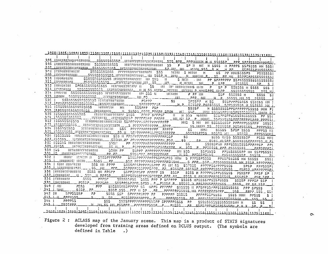
then combined as inputs to ACLASS and DCLASS runs, producing maps that
discriminated the following targets: conifers, hardwoods, and shaded
hardwoods. This map is shown in Figure 2; the categories, symbols used,and other information relevant to this map are shown in Table 1. The
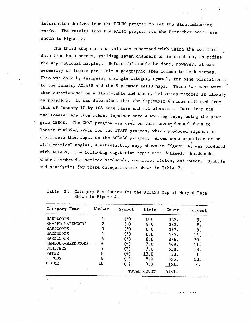
RATIO program was used with both scenes, to discriminate between conifersand non-conifers, using a ratio of channel 4 to channel 7 and using
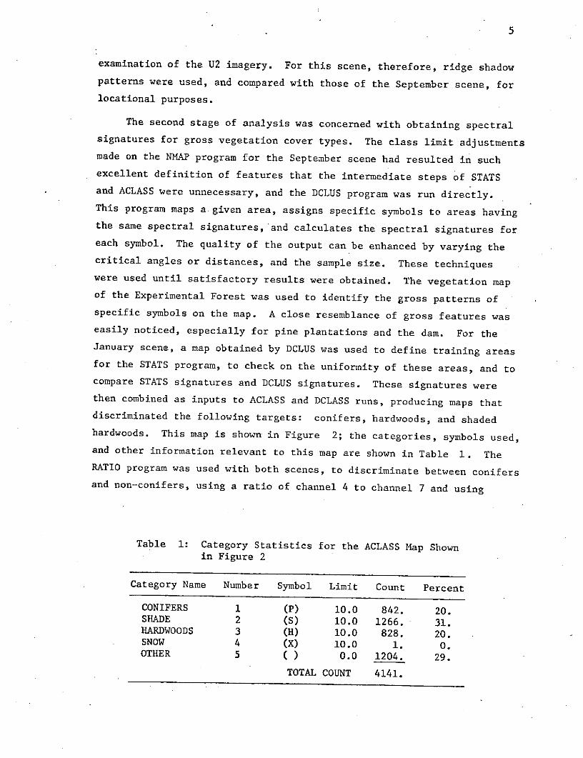
Table 1: Category Statistics for the ACLASS Map Shownin Figure 2
Category Name Number Symbol Limit Count Percent
CONIFERS 1 (P) 10.0 842. 20.SHADE 2 (S) 10.0 1266. 31.HARDWOODS 3 (H) 10.0 828. 20.SNOW 4 (X) 10.0 1. 0.OTHER 5 ( ) 0.0 1204. 29.
TOTAL COUNT 4141.
111.1 112DLUrrU111- 11 S .UZ- 1j.2L~13_jj3.rj 14n 11@SI1VlnI~ Il I I110 1 1] Arl1117nl I 17; 1 1 P n IW; I I I- S S. 3 SS 11 1 H T III iI I: 11 :H H 1
SOG ~ ~ ~ ~ O 0lHliii~ililllii .1'~ss ,s ii3iliiii5H S P SP 1H HH H SSSS IH PPPPS SSPSSSS HR SSSI.50 a.LJJIUJLLUIJIIIII -WI MIIil iI jIll Lij1~ 4J'411 rJ'I- ' HS 14 - PP Rnpr--PilIrelS L5C,,f' m~fllii'ililrSI (IIIIIIIIfIII i I 11 Vj 4 111! 11 SS5 Iii~III S HHHH. H SS PP RH iiSSSSPs PssssssI.5_rii I inIjij 1iii nflIL i i I~.SS 17111111 H 1414111-111 P nn PP R l sSPPSaaS S.SSSa j.5in I ill IiilH M ~ ~ SSS Ii~lilJli~ifh! HI S.SN ii S 1011 SSII SHM -iiiI PP SPPPPPPP SSPSSSSSSSSSSSSSSSI"111 iII i-j! :II 3S _ _ i10- - 11jil IM I li SH~512 11lI 1111111iii O PI'S 5S 55r S s ilflitii1ili:!l[ i H~ilII 11 S 1ii I! IIHIiIIIIIIIIIS iiWR P SP P 355555 H SSSS 555 I
T"~~l~lll Il 11' -311111P tj~isp , '' I514i IlMiilH 55.~S55 iiH'IINIiiiii Uill 055 G, 41 1 11:1411 P PP IH SSP SZSSSS H 5555 SI515L1)W - r 5 5 55 ., . . Li LUL.ili.. S -. _ S SS.SSJ.ic- ~5,~1t iH mp~p Ss SPSSPP 1H S 3 SG5PPPP5SSSS SS55SS Hfil~NUL!?233' -3.5_~3 S53 5 SHIUU2LL2III -- S 111P P Ps =W-Z-32~SS~5p 5assas SS 1iia.51.I355I 55 S HfHI~II H SSSPPP PSP SSSSP H SSSSSSSSPPSPPPPPppS55 RHH P)ill IM HIM1 11:itri1iiip:IH iiiiISSr) PPIP Si'PP:;P H H Sr53 HiMii Sr ,PPS3PP~S5SS5sS35S PP SSI
4~ ~ 1.1111 SiL IM HiHiSS SOSI Sl PPPPPPSGPP IS214 %7~; -. S:iiHS11i]iI:Hn PPPPri'PPPPPP PlP~ SS [11J1 iLSS S~P~SP SsS PPPSS .1525 lsrsss:":' 5 iii:pp~ ii Sin::: Hss npppppp SPP 35 in ss pP Ss PPPSSSII
, ~ I. Dii~i S.,. ii 0P2pp'pppp~ SS S Iss MISS SSSSSSSIP PSSG H I_5_1LSSS____ 11'] I:I i:LH1 VR -iJI.5ZI UL-PI J'1; )P 'lP3PP1~L2 SS52C ISSSSS liii:un:Pi~n~ 35! PppIpppi'pPPPPPPPIPPPPP SS GsSzssPn-ii PPPSSSSSSSSPPPPSP Pr'j_51n S's I:II!;!1 IN I ii 1 11 1111 HJLLSSJIJ P3 PLPpiPPPSO,3 5p2.EflE2 LsPP~a0 S5j_5RPPm2=S Js aa PSPa2530 1;5 1 WI WITs li[i:;I IM t1ii SSriM Pu' F:;rpp p"PrPPPPrpppp in sss sPSiSSs PPSSSSSS.SPP Im SSPpssss532 1 I II hiirirn : I:H~ GnSSPPPPPPP Sn ;pPPPrPPPPSGPP0sps1HI 111 PPIDSSPS0SSS0 PPSSPSS5SS RH SSSSS SSS I-533-1il~~~n i:i 11111.11.111_N] $P PPPPP PPPPRR2PSi UIjIfl_. pp , .P255p24SSSJHSp~~.534 1 IN IIijiifHIIINIii SS liii PPPP JsoPs PPPP31PPP PS Ili SS SZPSSS PPPPPSGPPPPSS~s SPSP PPPSSSPj3.3LnIJU1 IiLI~u!In.. S1-iL~~l5ppsspsp _Pp 555Prr ~ rrrp S S_52.JJP2PPRSJ536 11iiii:1,1HiMMIini 55 fll PP5PP SSPPS)PpPP PPPPP S5 SSSP SSS H PPPPP'SSPP3SSSSS PSSSPP PPSP SP I.3J1_LIU[L!W: 1U L I .SHL 2?S U 0S5J,p55 S a111P.P 0 S V ... P 2I--~ a-, S H PPPPPPPPPssI 7sse Ipp , ~531 '.iiiiiiiiuHP11 rn ppr r ~.p; rP) 555 PPP P SPPPPP SSSSS HPSSSSPPSSSPSSSS SSsSP PPPGP SSP I54() ( till PSSS PHI sSssipp 55 IllPs PPPPPP 535355"I 11 PPSPP5SI'PPSGSSSSSSSS PPP SPSSS5!aU ~ u1S~sL p s~ .PPP._ PR SP. PS RPPP.PRPSSSS.JII p.PPSP 2SP Rspp sss P- S SI5112 Ill SPPS1 spssp PP Sr1s SSP SPPP~P :;~PP PP PPPPPP SISSss PPPPPSSPSSSS SSSS HHH PPSSS S I5;114 IJ ----~ Us- 5 SPPPPP P P. p~ PP ppq!f 5 ' P P 1 qPppss PI'.-11 1111sssssssi iu s3J54...Z ) S SSSP.R LU&iL54P~PP PPPPPPSSPP PZPSSS PP 'Z S~h2SQS S P i wY e
I1 -5 1.1 01 12 111 1 11 rI. I I I 1 q I I I P I 0\
Figure 2 :ACLASS map of the January scene. This map is a product of STATS signaturesdeveloped from training areas defined on DCLUS output. (The symbols aredefined in Table .
-7
information derived from the DCLUS program to set the discriminating
ratio. The results from the RATIO program for the September scene are
shown in Figure 3.
The third stage of analysis was concerned with using the combined
data from both scenes, yielding seven channels of information, to refine
the vegetational mapping. Before this could be done, however, it was
necessary to locate precisely a geographic area common to both scenes.
This was done by assigning a single category symbol, for pine plantations,to the January ACLASS and the September RATIO maps. These two maps were
then superimposed on a light-table and the symbol areas matched as closely
as possible. It was determined that the September 6 scene differed from
that of January 10 by +68 scan lines and +81 elements. Data from the
two scenes were then subset together onto a working tape, using the pro-
gram MERGE. The UMAP program was used on this seven-channel data to
locate training areas for the STATS program, which produced signatures
which were then input to the ACLASS program. After some experimentation
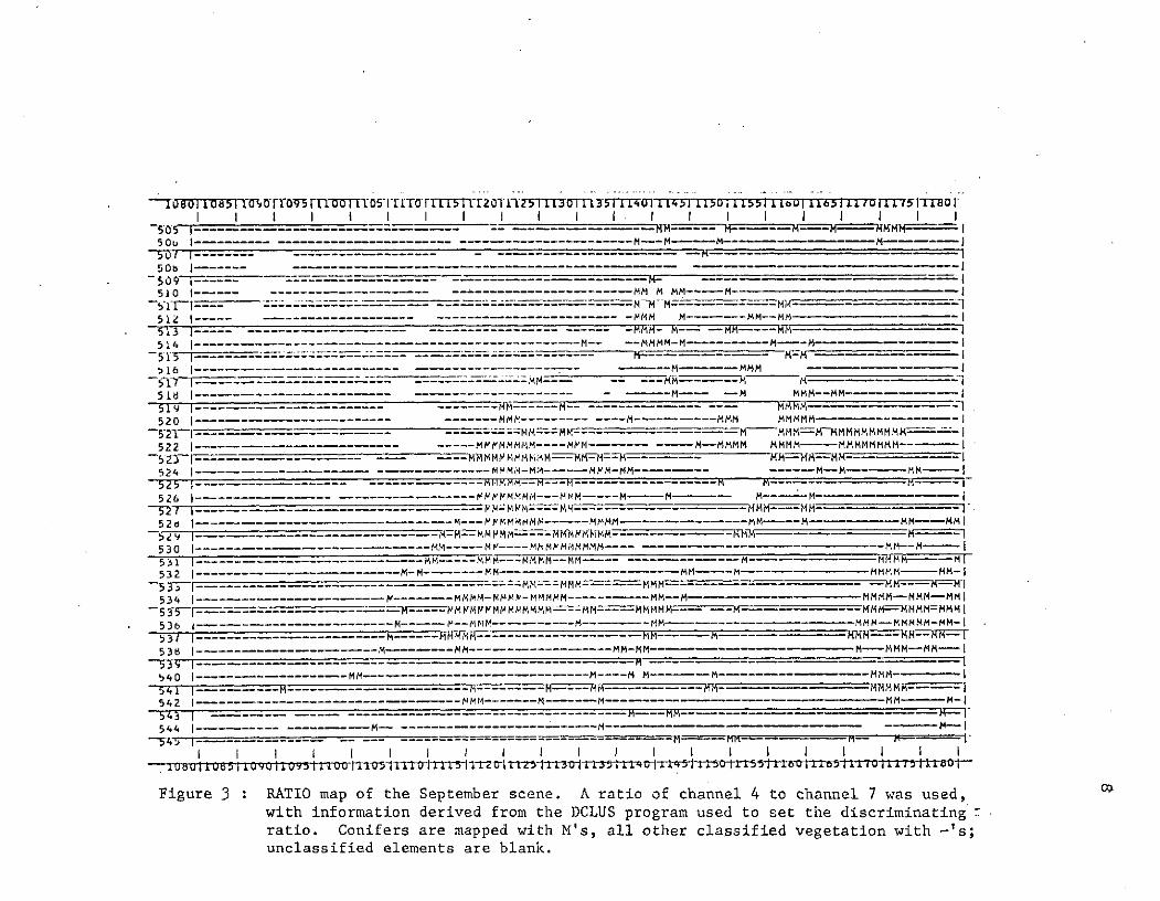
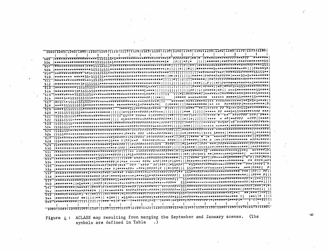
with critical angles, a satisfactory map, shown in Figure 4, was produced
with ACLASS. The following vegetation types were defined: hardwoods,shaded hardwoods, hemlock hardwoods, conifers, fields, and water. Symbols
and statistics for these categories are shown in Table 2.
Table 2: Category Statistics for the ACLASS Map of Merged DataShown in Figure 4.
Category Name Number Symbol Limit Count Percent
HARDWOODS 1 (*) 8.0 362. 9.SHADED HARDWOODS 2 (S) 8.0 331. 8.HARDWOODS 3 (*) 8.0 377. 9.HARDWOODS 4 (*) 8.0 473. 11.HARDWOODS 5 (*) 8.0 826. 20.HEMLOCK-HARDWOODS 6 (=) 7.0 469. 11.CONIFERS 7 (P) 7.0 538. 13.WATER 8 (+) 13.0 58. 1.FIELDS 9 (I) 8.0 556. 13.OTHER 10 ( ) 0.0 151. 4.
TOTAL COUNT 4141.
106 1001 T ot05FrO110o0rn-[L rrO110T t511Tr201 1123ILT30TL35 I11O1lrlT43 U i 1155 1i u T165711u 1S]Tt8 VI I I I I I I I I I I I I I I I I I 1 I I 1 1
50 1---- --------------------- M------- -------- NM N=-- I500 1--- ------- ------------------ ----- ------------------ M-------------- -
S-------- -------------------------------------50 I------- ----- --------- -------- ---
509 ------ ---------- - ----------------- -------------- -
510 1------ - ----------- N-------- M
1 1 ----------- ------------- M--MM513 ----- --------------- ------------------ --- -MMM- M--- ----- M--------
514 ----- ------------------ ----------- --- -MMMM-M---- M----M------------ 1
-515 1 - -- --- M
51 1- - ----------------- ------ M--- ------------------ --- MMM- I
522 I---M--.-......--- ------- ------- -- -- ---- N ---------- M------- -M --- MM---------I51 ----------------------- ------ MM-- ----- M-- M -------- ----- I518 T---------- ------------------ - --------- M -------------
520 I---------------------- ------- MM------M-- -------- ----MMM MMMM--- MM-------------I5 1 ---------------- ------ MM-- -- M------------- M MM- M MM-------
52 1---------- ----------------- ------- MM----------- -------- --- M MM-----MMM -- "--- I
522 -------------- ---- ---- MMMMMN M---MMMM--- ---- MMMM---MMMM- -- I
524 1------- -------- --------- ---M MMMMM---'I------ ----- MM-------MM--MMI
524 --------- - M- MMM-MM-----M-M------- M--- I
52 I------------------ ----------- MMMM------------------- M-----52 I----------------------- MM----N------M------- -M------------- ---
5 I ------ ------- - --------- ----- --- M--M-- MI
52 ----- --- M MM --------------------- nM- - ------------ MM- I530 I---------------------- ---- n ---- M.M, -5321 -------------------------- M---M-------M----M------------- - MN-N-I
532 I -------------------- "----N---- ------ -- N532 1 ------------------ -------- ------ MM----MM---------------------- -MM-MM- MA -
-5 31 -------- -'h------ --MMMMK5 5 1- ------------------- -M-M----- MMMMrin-M-----MMMMM-------M ---- KM===M I---- -
531 1 - ------- ------------- ------ -K-M- ---------------- M------------------ M--HM---1
538 1 ---------- -------- -------- M -------- --------- M-----------------M--n--
5 3 - - -- . fT540 MI- --------- ---------- M--1
540 |-------------------M M-----------------------------M M-------M-------- ---- H------ I
542 I -- - - Ai -- " M--- -
M-- -
541 ------------- --------------------- ---------M-------------------------- MMM-----I
542 1 --------------N--- --- - - -- I- ------ ------ ---- ----------------------- ------ M1--------- ?----
I I I B 1 1 6 1 1 1 I U I I 1 I I
Figure 3 : RATIO map of the September scene. A ratio of channel 4 to channel 7 was used,with information derived from the DCLUS program used to set the discriminatingratio. Conifers are mapped with M's, all other classified vegetation with -'s;unclassified elements are blank.
- 131DTO-8T0-9 11T1VM-T&Y5 Fl [0FrrT5TrI201l123fT30 TI33T4 1114!1115 T53=T6U T63TITIT5' ITSO I
IS, 5- a W WVI 4 fkV*S P P I P P -P I Ii
506 IPI Il*Pl* liIll******IPP*P*l*-%*p.*****SSl
510 1********~*I*S ******~~=~IITfi~
502 l* *****~SSSSS *****~*~PP*IIiII *1I****=******** j****j
51 1 1 15.~~ 1 1 1 1 1 *1 1~ 1 U 1 1 I wwq IiT*W *f*T*i P I
512
513 i**S*ssss**********SsSS* ********* * **PII*I 1*** ...... S=**S***
518 I-**S=SSSSSSSSSS***********u ******~**SS=***PP jj++jj j***** *=**** ++++4
519**~* ***illj=*P **Il ... PP +*+====...3S~**
510 I*SSSSSSSSSS*** * ****I. l*S ****SPP *PP==ll lJlil 111111+++++ P - PPPPO***#***P *
522 IS**SSSSSSSS**********w**II l *S**P*II[11Ip..** *Il jlll+*++ PIP =PSSS* .*l
520 ISSSSSSSSSSS************** II I*S*PPPPPPl*=PP...III I* ** I IIl+++++ PP **==S=S*******P****jI
525T35 *7 S'P S I IrT ==~ PP = - P1P P PPI 11 t11 pf**p *++ I
522 ISSSSSSSS= ********* *SO**P PPP =PPP.PPPP**IlIIllIlllll++++ ... ==pP P~l
528. PIPPP PP-PPP=*P PPPI ll lp** ~Ii * 1*IP.**** I+*+*++ I
526 lSS****** ********* ***~*IPI**P PPf pp~pppp***lPIII*l*****II++ .I****~*ll~**
532 l****Itl******SS* * PPPIISPPPP=*pp=== Ijps**jJ= l*IPP***** =P*=**pPI
534 5 FP*P= ~ ~PPPI*( [jl-**=.PP* .*p ***TPP PP*IPj
536 1 P****~~ ***pP I *-PI = I*IPPP I*SI I~ I SS* P=P - S*** .=***IjP
532 **P*PI* *=*-SP PFPP *P ppp ==p**Il* SS**P=. ****=**S****-** I I P I IPP I
536 l******w************PIl** P***.=P=p*IP=S*pPPI **PPll SS P=P *** *jPPill
539 1*** *****S***p=I** p =~**~*PPP*55** -P====***** ...... PI .P
541 1 v * I I IF~z * v * I w= = ===-j~f 5 **PTT* n 1d
54Z I****,*~**==-*PP**P* I ===**PPSPP*PP=PPPP*IPPPPPPP==SSSa **PP=* ********1I** P**.III Il
543I* * 1~* * I **j I I 1 446 1*~ 1 **I* 1P1-
544 l***PP=P **I II *I Il I SS*Pz= sPpp*S*.****PPP*SSSS**PP**. . ******* .I .l1 I
I I I I I I I I I I I I I I I I I II U U 0 1 8 5 1 TO L9 011T it1 tt0l - I ITj-nj t-rMI r -z 0I 11 t -1113 0- -tit 1-r4-T5 1 1 151 1 1 01 -
Figure 4 :ACLASS map resulting from merging the September and January scenes. (The
symbols are defined in Table .
10
Ground truth, in the form of maps, underflight photography, and a
visit to the field area, was used to check the final map produced by the
ACLASS program from the merged data. The USGS 7 1/2 minute topographic
map was practically the same scale as the digital printout, facilitating
the transfer of stream systems and roads to an overlay on the computer
map. This map was then compared to the U2 and large-scale underflight
photography, and to the vegetation map of the experimental forest. A
half-day field inspection of the test area further refined the comparison
with ground truth.
Results
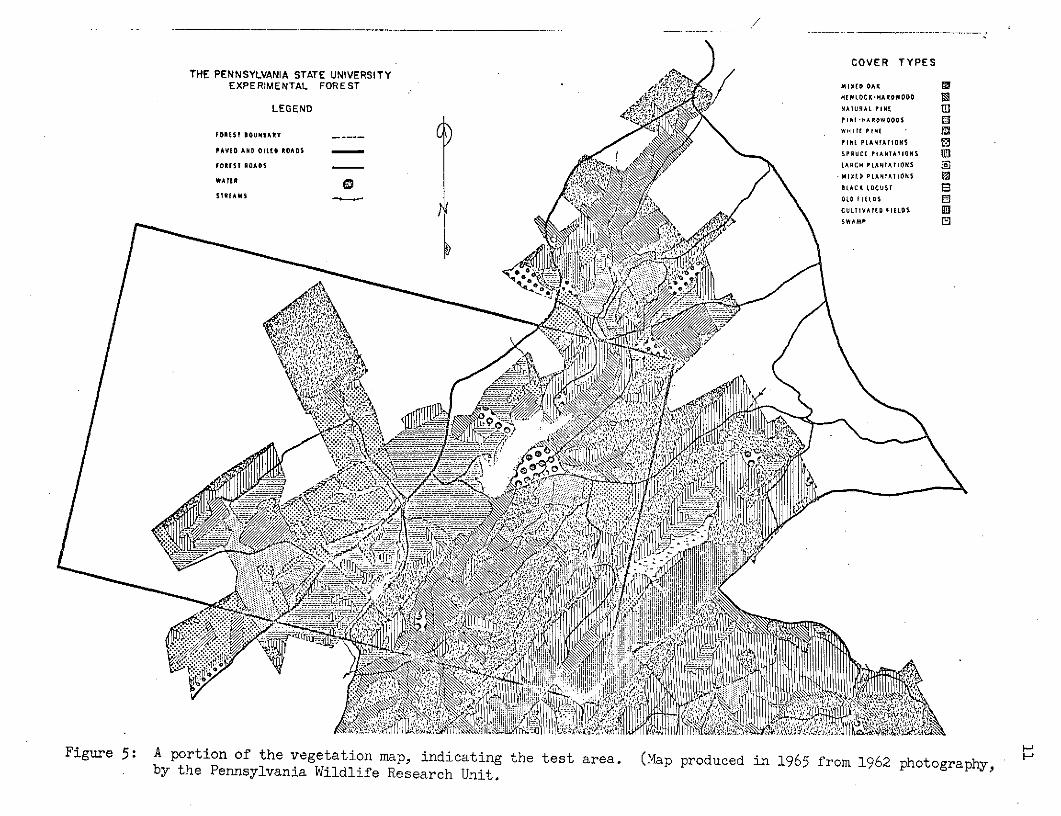
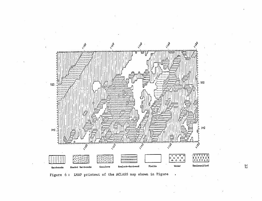
Comparison of the vegetation map (Figure 5 ) with an LMAP printout
of the ACLASS map from the merged data (Figure 6 ) indicates the accuracy
that has been achieved in mapping vegetation classes in the test area by
this method. The following results from this study have been realized:
1. Three ORSER programs (RATIO, ACLASS, and DCLUS) were able
to isolate and map coniferous forest vegetation provided the conifers
occurred in blocks of approximately five acres or more and comprised the
bulk of the vegetation in those blocks. This was verified by ground
truth, and was achieved on both summer and winter scenes.
2. The merging of winter and summer scene data made it possible
to differentiate hardwoods with coniferous understory from hardwoods on
the one hand and conifers on the other. This possibly was suggested when
it was observed that conifers occurred in some areas in the winter scene
maps which had been classified as hardwoods in the summer scenes. This
area of apparent confusion was verified, by field-checking, as being
hardwoods with an understory of hemlocks.
3. Discrimination between coniferous species on the basis of
spectral characteristics alone does not appear very promising. However,
where a particular species is associated with another vegetation type,
discrimination is possible. Thus, hemlocks with hardwoods can be dif-
ferentiated from coniferous plantations, and it seems likely that Virginia
pine and table mountain pine on old fields can be also defined as a
COVER TYPESTHE PENNSYLVANIA STATE UNIVERSITY,_,
EXPERIMENTAL FOREST MIXED OAKAH[MLOCK-HARDWOOD
LEGEND NATURAL PINE EPINE-MARDWOODS
FOREST BOUNDARY wPINE PLANTATIONS 0
PAVED AND OlfED ROADS SPRUCE PLANTATIONS [
FOREST ROADS LARCH PLANTATIONS ra
MtIXD PLANTATIONSWATER
BLACK LOCUST E3STREAMS - OLO FIELDS
CULIVATED FIELDS l
1 7
'Y'
Figure 5: A portion of the vegetation map, indicating the test area. (Map produced in 1965 from 1962 photography, Hby the Pennsylvania Wildlife Research Unit.
~"~ c :::::~0
VI11
~f~7IA
ION 1111y; ,; 1-
,, IN
F i g r e 5 : A o r i o o t e eg t a i o m a , nd c a i n t e e s a e a ( a p p r o u c d n 9 6 f o m 19 2 h o og a p y ,by hePensyvaiaWillie eserc Uit
//////////// ,// III0
/////// , 1Ir2 // // ,, 11 1- //// // i xII i
/. .t .. .. ... ..
/// ~
////
%'=F,'d I I
- //
:::tXX
A,
.' + Ix h , I
+ _+ + rx-777+ C~+ x x x
~~1 1
Hardvoods Shaded lardwoods Conifers Remlock-Hardwood Fields Water Onclassified
Figure 6 : LMAP printout of the ACLASS map shown in Figure .
13
separate category. However, the separation of spruce plantations fromred pine plantations does not appear promising.
4. Discrimination between hardwood types in this scene doesnot appear very promising when using only winter and summer data, exceptwhere these types are characterized by association with evergreen species.The addition of spring and fall data may help. However, variation inhardwood type within the test area is not great.
5. Although major ridges do not occur within the experimentalforest, their presence in the mapped scenes indicates potential problemsin matching vegetation signatures in the shaded areas with signatures ofthe same vegetation type under open light. This is to be further inves-tigated.
6. Clear-cut areas of more than 20 acres in size were easilydetected by computer processing.
Conclusions
By computer processing of ERTS-1 tapes it is possible to identifyand map major forest types. The precision of classification appears tobe such that it could serve as a useful first stage of a multi-stagesampling scheme for forest inventory. Refinement of vegetation typeidentification is made possible by using merged data from differentseasonal overpasses. Before this preliminary phase can be consideredcompleted, however, further work is needed to explore additional refine-ments of classifications, to statistically analyze classification accu-racy, and to develop procedures for classifying shaded vegetation.
ORSER-SSEL Technical Report 16-73The Pennsylvania State UniversityMay 1973
Recommended