Research Division Federal Reserve Bank of St. Louis Working Paper Series
Lucas meets Baumol and Tobin
Yi Wen
Working Paper 2010-014B http://research.stlouisfed.org/wp/2010/2010-014.pdf
June 2010 Revised October 2010
FEDERAL RESERVE BANK OF ST. LOUIS Research Division
P.O. Box 442 St. Louis, MO 63166
______________________________________________________________________________________
The views expressed are those of the individual authors and do not necessarily reflect official positions of the Federal Reserve Bank of St. Louis, the Federal Reserve System, or the Board of Governors.
Federal Reserve Bank of St. Louis Working Papers are preliminary materials circulated to stimulate discussion and critical comment. References in publications to Federal Reserve Bank of St. Louis Working Papers (other than an acknowledgment that the writer has had access to unpublished material) should be cleared with the author or authors.

Lucas Meets Baumol and Tobin�
Yi WenFederal Reserve Bank of St. Louis
&Tsinghua University
First Version: October 2009
This Version: October 17, 2010
Abstract
Many issues that were traditionally analyzed using the Baumol-Tobin model can also be
analyzed, perhaps more easily, using the Lucas (1980) cash-in-advance model where money
serves both as a medium of exchange and as a store of value. This is illustrated by three
examples (implications) of the Lucas model: (i) the velocity of money is time varying, volatile,
and in�ation-dependent; (ii) transitory money injections have expansionary real e¤ects on output
and employment; and (iii) the welfare cost of anticipated in�ation is a couple of orders larger
than the conventional estimates.
Keywords: Cash-in-Advance, Distribution of Money Demand, Velocity, Welfare Costs of
In�ation.
JEL codes: E12, E13, E31, E32, E41, E43, E51.
�This paper is based an earlier version titled "When does heterogeneity matter?" I thank Tom Cooley, NarayanaKocherlakota, Nancy Stokey, Pengfei Wang, and Mike Woodford for comments, Luke Shimek for research assistance,and Judy Ahlers for editorial assistance. The usual disclaimer applies. Correspondence: Yi Wen, Research De-partment, Federal Reserve Bank of St. Louis, P.O.Box 442, St. Louis, MO, 63166. Phone: 314-444-8559. Fax:314-444-8731. Email: [email protected].
1

1 Introduction
Many important issues in applied monetary theory that have been analyzed traditionally using the
Baumol (1952) and Tobin (1956) model can also be analyzed, perhaps more easily, using the Lucas
(1980) model. In particular, it is shown that allowing money to serve as a store of value in addition
to a medium of exchange can lead to dramatically di¤erent implications of monetary policies, in
contrast to standard cash-in-advance (CIA) models. These di¤erences include the following: (i) The
velocity of money is highly variable in response to environmental changes, in contrast to the �ndings
of Hodrick, Kocherlakota, and Lucas (1991) based on a representative-agent CIA framework. (ii)
Transitory lump-sum monetary injections have expansionary e¤ects on aggregate consumption,
employment, and output. (iii) Anticipated in�ation is potentially very costly: with a su¢ ciently
strong precautionary motive for cash holdings to match the interest elasticity of aggregate money
demand in the United States, households are willing to give up 10% to 15% of consumption to
avoid 10% annual in�ation, in sharp contrast to the �ndings of Cooley and Hansen (1989), Lucas
(2000), and others in the literature based on the representative-agent assumption.1
The key feature of the Lucas (1980) model, in contrast to standard CIA models, is that there
exists a precautionary motive for holding money (because of uninsured idiosyncratic preference
shocks) and thus a well-de�ned and endogenously determined distribution of money balances in
equilibrium, as in the Baumol-Tobin model. All of the aforementioned implications of the Lucas
model are generated through the responses of this endogenous distribution of money demand to
monetary policy changes.
For example, there are three factors contributing to the large welfare cost of in�ation in the
Lucas model: (i) Precautionary money demand motivates agents to hold excessive amounts of cash
to avoid liquidity (CIA) constraints, and agents with large money holdings su¤er disproportionately
more from in�ation tax than do agents with smaller real balances. (ii) The fraction of the population
with a binding CIA constraint increases with in�ation. This especially hurts those with the greatest
urge to consume and generates additional welfare costs along the extensive margin. (iii) In addition,
as in Cooley and Hansen (1989), agents opt to switch from "cash" goods (consumption) to "credit"
goods (leisure), thereby reducing labor supply and aggregate output. These e¤ects together yield
a much larger welfare cost of in�ation compared to that in representative-agent CIA models where
only the third factor operates.
However, the most crucial factor is the sensitivity of the distribution of money demand (or
1E.g., also see Dotsey and Ireland (1996).
2

aggregate velocity) to policy and environmental changes. CIA constraints are e¤ectively borrowing
constraints and such constraints do not always bind. So aggregate velocity is linked to the dis-
tribution of money demand because cash-poor agents spend money more "quickly" than cash-rich
agents when in�ation rises and the portion of cash-poor agents also increases with in�ation. This
link between velocity (or the distribution of money demand) and in�ation has important welfare
consequences. As noted by Aiyagari (1994, 1995) and Huggett (1993, 1997) in real models, un-
der borrowing constraints agents have strong incentives to self-insure against idiosyncratic shocks
through precautionary savings. Hence, in equilibrium the probability of a binding borrowing con-
straint, or the proportion of the liquidity-constrained population, is very small. This implies that
heterogeneous consumers are su¢ ciently self-insured and their consumption level behaves like that
of the median or representative agent. However, the same precautionary-saving mechanism works
against these individuals when the chief means of saving is money, because the motive for self-
insurance implies that agents opt to hold too much cash in hand to avoid a binding CIA constraint.
Thus, they would be heavily taxed by in�ation unless they could rapidly reduce money holdings as
in�ation rises. However, although reducing money demand can lower the in�ation tax, it creates
another cost: The portion of liquidity-constrained population increases. This raises the welfare
cost of in�ation along the extensive margin because liquidity-constrained agents must face a higher
variance of consumption than nonconstrained agents.2
The aggregate economy reacts positively to transitory monetary shocks because monetary in-
jections stimulate consumption for liquidity-constrained individuals but not for cash-rich agents;
thus, the aggregate price level does not move one for one with aggregate money supply. In addi-
tion, under precautionary saving motives, money demand will increase more than proportionately
with consumption, which induces labor supply to rise so that income can increase su¢ ciently to
satisfy both the higher consumption and the higher money demand. These together imply that the
aggregate price level appears "sticky", the velocity of money is countercyclical (because aggregate
money demand rises more than consumption), and money has expansionary e¤ects on aggregate
employment and output.3 This is in sharp contrast to representative-agent CIA models where the
velocity is constant, prices move nearly one for one with money injections, and monetary shocks
are contractionary.4
Since the original Lucas (1980) model is not analytically tractable under standard constant-
2 Imrohoroglu (1992) noted that a similar mechanism in the Bewley (1980) model can lead to a large welfare costof in�ation. However, the fraction of the population with a binding liquidity constraint is �xed in her model, leadingto a smaller welfare cost of in�ation than is implied by this model. See Wen (2009) for more discussions on this issue.
3Based on a Baumol-Tobin inventory-theoretic model with heterogeneous money demand, Alvarez, Atkeson, andEdmond (2008) also noted that velocity is countercyclical and aggregate price is "sticky" under monetary shocks.
4For the monetary literature based on the Baumol-Tobin model, see Jovanovic (1982), Grossman and Weiss (1983),Rotemberg (1984), Romer (1986), and Chatterjee and Corbae (1992). For the more recent literature, see Alvarez,Atkeson and Kehoe (1999), Alvarez, Atkeson and Edmond (2008), Chiu (2007), and Khan and Thomas (2006), amongothers.
3

relative-risk-aversion (CRRA) utility functions, representative-agent versions of this model are rou-
tinely used in the literature for monetary-policy and business-cycle analyses (see, e.g., Lucas, 1984;
Lucas and Stokey, 1987; and Cooley and Hansen, 1989; among many others). However, under
indivisible labor (or quasi-linear preferences), the Lucas (1980) model can be made analytically
tractable and the equilibrium distribution of money demand can be characterized by closed forms.5
Consequently, both the short-run and long-run implications of monetary policies can be examined
by standard solution methods available in the real-business-cycle (RBC) literature without the need
to rely on numerical methods (such as Krusell and Smith, 1998). Analytical tractability not only
reduces computational costs but also makes the model�s mechanisms transparent.
In a separate paper (Wen, 2009), I study welfare implications of monetary policies in a gen-
eralized Bewley (1980) model where money serves solely as a store of value and is not required
as a medium of exchange. There I show that anticipated in�ation can also be extremely costly
when the model is calibrated to match the distribution of household money demand in the data.
The major di¤erences between Wen (2009) and this paper include the following: (i) A monetary
equilibrium does not always exist in the model of Wen (2009) especially if the rate of in�ation is
su¢ ciently high, whereas agents must hold money for transaction purposes in the Lucas (1980)
economy even under hyperin�ation. (ii) The velocity of money can be in�nity in a Bewley economy
but bounded above by unity in the Lucas (1980) economy. In addition, Wen (2009) considers idio-
syncratic wealth shocks, which are more di¢ cult to self-insure than preference shocks. For these
di¤erences, there is no a priori reason to expect the implications of monetary policies be the same
in the two economies. An independent methodological contribution of this paper is to make the
Lucas (1980) model analytically tractable.
This paper is also related to a recent strand of the monetary literature that studies the welfare
implications of in�ation in heterogeneous-agent models with incomplete markets and borrowing
constraints.6 In particular, Algan and Ragot (2010) show that the long-run neutrality of in�ation
on capital accumulation obtained in complete market models no longer holds when households
face binding credit constraints. In their model, borrowing-constrained households are not able
to rebalance their �nancial portfolio when in�ation varies, and thus adjust their money holdings
di¤erently compared to unconstrained households. This heterogeneity leads to a precautionary
savings motive, which implies that in�ation increases capital accumulation, à la Aiyagari (1994).
A fundamental modeling di¤erence between Algan and Ragot (2010) and this paper is that they
derive money demand by assuming money in the utility function. In addition, the asset that
5 It is noted by Stokey and Lucas (1989, ch13.6-7) that the Lucas model is analytically tractable with a linearutility function in consumption. In this paper, I follow Wen (2009) and consider CRRA utility functions (e.g., logutility).
6See, e.g., Akyol (2004), Algan and Ragot (2010), Boel and Camera (2009), Erosa and Ventura (2002), Telyukovaand Visschers (2009), among others.
4

provides self-insurance in their model is capital, instead of money (as in this paper).
In many aspects my model may appear isomorphic to the search model of Lagos and Wright
(LW, 2005) for the following reasons: (i) My model assumes quasi-linear preferences to achieve
analytical tractability. (ii) My model has two subperiods in every time period� labor supply and
capital investment are determined in the �rst subperiod and money demand and consumption
are determined in the second subperiod. (iii) LW also �nd much larger welfare cost of in�ation
then the representative-agent monetary literature (e.g., Cooley and Hansen, 1989; Lucas, 2000).
But the similarities may be more super�cial than substantive. First and most importantly, the
motives for holding money are fundamentally di¤erent in the two models. There is no lack of
double coincidence (or search friction) in my model, which is the key physical environment in LW
to motivate money demand as a medium of exchange. In contrast, even though CIA constraints are
imposed, the main function of money in my model is a store of value that provides self insurance
against idiosyncratic shocks (as in Bewley, 1980; Svensson, 1985). Consequently, all trades take
place in centralized markets and there is no need to assume consumers to have two utility functions
in the two subperiods (which is the case in LW). Second, there exists a well de�ned and analytically
tractable distribution of money holdings in my model, whereas money distribution in the LW model
is not analytically tractable without a sequential centralized market and it becomes degenerate
under quasi-linear preferences. Third, my model has a standard neoclassical DSGE environment
with capital accumulation whereas capital is absent in the LW model. Because of these di¤erences,
there is no reason to expect a priori that the two models generate similar results. As emphasized
by LW, search frictions are critical to obtaining their large welfare results; yet the welfare cost of
in�ation in my model is several times larger than found in LW. Nonetheless, in many aspects one
may re-interpret the model as a stochastic version of the LW model with anonymous centralized
trading in both the �rst and second sub-periods. Since not much work has been done to study
quantitatively the short-run dynamics in the LW model, not all of the results in the two papers are
directly comparable and it remains an interesting research topic to formally establish the equivalence
of the two models.7
The rest of the paper is organized as follows. Section 2 presents the benchmark model and
shows how to obtain closed-form decision rules for money demand at the individual level. Section
3 characterizes general equilibrium. Section 4 presents a representative-agent version of the model
(as the control model) to further highlight the critical role played by the distribution of money
demand. The implications of heterogeneity are studied and compared with those of the control
model in Sections 5 through 8. Section 9 concludes the paper.
7A recent literature has extended the LW framework to incorporate capital accumulation and uninsured idio-syncratic risk. See, e.g., Aruoba and Wright (2003) and Aruoba, Waller, and Wright (2009) for how to introduceneoclassical �rms and capital accumulation into the LW framework, and Telykova and Visschers (2009) for how tointroduce uninsured idiosyncratic uncertainty (and the literature therein).
5
2 The Model
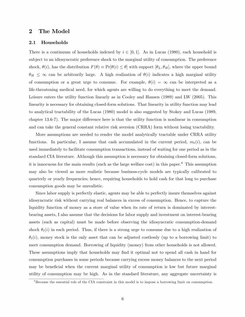
2.1 Households
There is a continuum of households indexed by i 2 [0; 1]. As in Lucas (1980), each household issubject to an idiosyncratic preference shock to the marginal utility of consumption. The preference
shock, �(i), has the distribution F (�) � Pr[�(i) � �] with support [�L; �H ], where the upper bound�H � 1 can be arbitrarily large. A high realization of �(i) indicates a high marginal utility
of consumption or a great urge to consume. For example, �(i) = 1 can be interpreted as a
life-threatening medical need, for which agents are willing to do everything to meet the demand.
Leisure enters the utility function linearly as in Cooley and Hansen (1989) and LW (2005). This
linearity is necessary for obtaining closed-form solutions. That linearity in utility function may lead
to analytical tractability of the Lucas (1980) model is also suggested by Stokey and Lucas (1989,
chapter 13.6-7). The major di¤erence here is that the utility function is nonlinear in consumption
and can take the general constant relative risk aversion (CRRA) form without losing tractability.
More assumptions are needed to render the model analytically tractable under CRRA utility
functions. In particular, I assume that cash accumulated in the current period, mt(i), can be
used immediately to facilitate consumption transactions, instead of waiting for one period as in the
standard CIA literature. Although this assumption is necessary for obtaining closed-form solutions,
it is innocuous for the main results (such as the large welfare cost) in this paper.8 This assumption
may also be viewed as more realistic because business-cycle models are typically calibrated to
quarterly or yearly frequencies; hence, requiring households to hold cash for that long to purchase
consumption goods may be unrealistic.
Since labor supply is perfectly elastic, agents may be able to perfectly insure themselves against
idiosyncratic risk without carrying real balances in excess of consumption. Hence, to capture the
liquidity function of money as a store of value when its rate of return is dominated by interest-
bearing assets, I also assume that the decisions for labor supply and investment on interest-bearing
assets (such as capital) must be made before observing the idiosyncratic consumption-demand
shock �t(i) in each period. Thus, if there is a strong urge to consume due to a high realization of
�t(i), money stock is the only asset that can be adjusted costlessly (up to a borrowing limit) to
meet consumption demand. Borrowing of liquidity (money) from other households is not allowed.
These assumptions imply that households may �nd it optimal not to spend all cash in hand for
consumption purchases in some periods because carrying excess money balances to the next period
may be bene�cial when the current marginal utility of consumption is low but future marginal
utility of consumption may be high. As in the standard literature, any aggregate uncertainty is
8Because the essential role of the CIA constraint in this model is to impose a borrowing limit on consumption.
6

resolved at the beginning of each period and is orthogonal to idiosyncratic uncertainty.
An alternative setup of the model�s information structure for decision-making is as follows.
Each time period is divided into two subperiods. The preference shock �t(i) is realized only in the
second subperiod. In the �rst subperiod, after aggregate shocks are realized, household i chooses
labor supply nt(i) and a nonmonetary asset st(i) that pays the real rate of return rt > 0. In the
second subperiod, after the idiosyncratic shocks are realized, the household chooses consumption
ct(i) and nominal balance mt(i) to maximize utility subject to a liquidity (CIA) constraint.
De�ne
xt(i) �mt�1(i) + �� t
Pt+Wtnt(i) + (1 + rt)st�1(i)� st(i) (1)
as the cash in hand of household i, which includes real cash balances carried over from the previous
period plus any lump-sum transfers, mt�1(i)+� tPt
, labor income, Wtnt(i), and capital gains net of
investment in the nonmonetary asset, (1 + rt) st�1(i)� st(i); where Pt denotes aggregate price, Wt
the real wage, and �� t a lump-sum per capita nominal transfer. Taken as given the macroeconomic
variables fPt;Wt; rt; �� tg, household i�s problem can thus be expressed compactly as9
maxfc;mg
E0
(maxfn;sg
~E0
( 1Xt=0
�t [�t(i) log ct(i)� ant(i)]))
subject to
ct(i) +mt(i)
Pt� xt(i) (2)
ct(i) �mt(i)
Pt; (3)
where the operator ~Et denotes expectations conditional on the information set of period t excluding
the idiosyncratic shocks �t(i), whereas the operator Et denotes expectations conditional on the full
information set of period t including �(i). Without loss of generality, assume a = 1 in the utility
function.
Note the following important features of the model:
(i) Cash in hand, xt(i), is predetermined in the second subperiod (after �t(i) is realized) be-
cause labor supply and asset investment are chosen in the �rst subperiod without observing �t(i).
A question thus naturally arises: Would the CIA constraint in equation (3) always bind, as in
representative-agent CIA models? The answer is "No." In fact, how often the CIA constraint may
bind in this model depends crucially on labor supply and the anticipated in�ation rate � the cost
9The model remains analytically tractable even if the period-utility function takes the more general CRRA form,
u(c; n) = �t(i)ct(i)
1� �11� � ant(i).
7

of holding money. If the in�ation rate is low, the CIA constraint may rarely bind because the
household can almost fully self-insure itself against random liquidity-demand shocks by working
harder and accumulating more cash in the �rst subperiod. On the other hand, if holding cash is too
costly because of high in�ation, the CIA constraint may bind frequently because the household opts
to reduce real balances by working fewer hours. Hence, the probability of a binding CIA constraint
depends on the distribution of �(i) and the in�ation rate.
(ii) In anticipating that the CIA constraint may or may not bind in the second subperiod, the
household opts to choose labor supply in the �rst subperiod optimally based on expected in�ation
and the distribution of �t(i) so that the level of cash in hand is optimal ex ante, although ex post
the actual cash in hand may be below or above what is required to satisfy the realized liquidity
demand determined by �t(i).
(iii) Since preference shocks are i.i.d. and the marginal cost of labor supply is constant, house-
holds can adjust hours worked (labor income) elastically to target any optimal level of cash in
hand (xt(i)) regardless of the initial wealth level (mt�1(i)Pt
+ (1 + rt) st�1(i)). In such a case, indi-
vidual history (such as mt�1(i) and st�1(i)) no longer matters and households can all start the
second subperiod with the same optimal amount of cash in hand when making consumption and
money-holding decisions. This property simpli�es the model tremendously and makes the model
analytically tractable.10
De�ne St as household i�s state space that includes all predetermined variables and exogenous
shocks but excludes �it (we use �i and �(i) interchangeably). With this notation, labor supply
can be denoted as nt(i;St) because it is independent of �it. Denoting��t(i;St; �
it); vt(i;St; �
it)as
the Lagrangian multipliers for constraints (2) and (3), respectively, the �rst-order conditions for
{ct(i;St; �it); nt(i;St); mt(i;St; �t); st(i;St; �t)} are given, respectively, by
�t(i)ct(i;St; �t)�1 = �t(i;St; �t) + vt(i;St; �t) (4)
1 =Wt~E [�t(i;St; �t)] (5)
�t(i;St; �t)
Pt= �Et
�t+1(i;St+1; �t+1)
Pt+1+vt(i;St; �t)
Pt(6)
~E [�t(i;St; �t)] = �Et [(1 + rt+1)�t+1(i;St+1; �t+1)] ; (7)
where the operator ~E in equations (5) and (7) re�ects the fact that labor supply and asset investment
must be chosen in the �rst subperiod before observing the idiosyncratic shock �t(i). By the law
10This property is reminiscent of Lagos and Wright (2005).
8
of iterated expectations and the orthogonality assumption of aggregate and idiosyncratic shocks,
equations (6) and (7) can be rewritten as
�t(i;St; �t) = �Et
�PtPt+1
~E [�t+1(i;St+1; �t+1)]
�+ vt(i;St; �t) = �Et
PtPt+1Wt+1
+ vt(i;St; �t) (8)
1
Wt= �Et
h(1 + rt+1) ~E [�t+1(i;St+1; �t+1)]
i= �Et
1 + rt+1Wt+1
; (9)
where the �rst equality in each of the above two equations applies the law of iterated expectations
and the orthogonality condition, and the second equality in each of the above two equations uses
equation (5).
In a steady state without aggregate uncertainty, Wt = W and rt = r; hence, equation (9)
implies 1 = � (1 + r), a standard relationship for interest-bearing assets. Hence, unlike Aiyagari
(1994), this model does not have the "over accumulation of capital" problem because there are no
precautionary saving motives for capital, so taxing capital is not optimal here. As shown below,
however, taxing money holdings (by in�ation) is not optimal either despite the precautionary saving
motive for real balances.
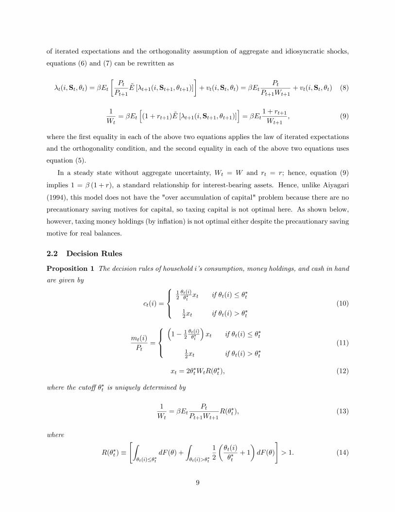
2.2 Decision Rules
Proposition 1 The decision rules of household i�s consumption, money holdings, and cash in hand
are given by
ct(i) =
8><>:12�t(i)��txt if �t(i) � ��t
12xt if �t(i) > ��t
(10)
mt(i)
Pt=
8><>:�1� 1
2�t(i)��t
�xt if �t(i) � ��t
12xt if �t(i) > ��t
(11)
xt = 2��tWtR(�
�t ); (12)
where the cuto¤ ��t is uniquely determined by
1
Wt= �Et
PtPt+1Wt+1
R(��t ); (13)
where
R(��t ) �"Z
�t(i)���tdF (�) +
Z�t(i)>�
�t
1
2
��t(i)
��t+ 1
�dF (�)
#> 1: (14)
9
Proof. See Appendix.
These decision rules are economically very intuitive. Both consumption and saving are propor-
tional to cash in hand xt but with the marginal propensity to consume (and the marginal propensity
to save) state-dependent. When the urge to consume is high (�(i) > ��), total cash in hand is split
perfectly between consumption and cash (because cash is needed to purchase consumption goods);
so the marginal propensity to consume is 12 , as in a standard representative-agent CIA model.
When the urge to consume is low (�(i) < ��), less than half of the total cash in hand is allocated
to consumption, more than half is allocated to saving; so the marginal propensity to consume is
12�t(i)��t
< 12 , and consumption comoves perfectly with preference shocks and saving absorbs any extra
cash in hand not spend. Hence, saving (money demand) is a bu¤er stock.
The probability of a binding liquidity constraint is given by F (��t ), which is endogenously and
optimally determined by each household according to the macroeconomic states because the cuto¤
is determined by equation (13). The determination of the optimal cuto¤ is thus related to the
determination of optimal cash in hand, which in turn is related to the optimal labor supply (or
wage income).
The function R(��) in equation (13) measures the (shadow) rate of return to liquidity (or
cash inventory). The left-hand side of equation (13) is the opportunity cost of holding one more
unit of real balances as inventory instead of one more unit of real capital asset. The right-hand
side is the expected real returns to money, which takes two possible values: The �rst is simply
the discounted next-period utility cost of inventory (�Et PtPt+1Wt+1
) in the case of low liquidity
demand (� � ��), which has probabilityR�(i)��� dF (�). The second is the marginal utility of
consumption ( �t(i)��t�Et
PtPt+1Wt+1
) in the case of high liquidity demand (� > ��), which has probabilityR�(i)>�� dF (�). The optimal cuto¤ �
�t (or labor income) is chosen so that the marginal cost equals
the expected marginal gains. Hence, the rate of return to inventory investment in money (liquidity)
is determined by R(��t ). Notice that R(��t ) > 1 as long as �
�t < �H . That is, the liquidity premium
R(��) exceeds 1 as long as the probability of being cash constrained is strictly positive. The fact
that R > 1 implies that the option value of one dollar exceeds 1 because it provides liquidity in the
event of a high urge to consume. This inventory-theoretic formula of the rate of return to liquidity
is similar to that derived by Wen (2008, 2009) in di¤erent models.
Equations (13) and (14) imply that the cuto¤ ��t is independent of i under the assumption that
�(i) is i.i.d. Equation (12) then implies that the optimal cash in hand, xt(i), is also independent of
i. The intuition for xt to be independent of i is as follows: (i) xt is determined before the realization
of �t(i) and agents face the same distribution of �(i) when choosing xt. (ii) The marginal cost of
10

leisure is constant; hence, labor is elastically supplied. Therefore, labor income can be adjusted
elastically through labor supply to target any optimal level of cash in hand that balances the
expected marginal costs and bene�ts of carrying money. In other words, since the expected bene�ts
and costs of holding one extra dollar depend only on the distribution of �(i) and macro variables
that individuals take as given, and since labor can be adjusted elastically with constant marginal
utility cost, all households opt to choose the same target level of cash in hand regardless of their
initial wealth. In other words, such a target policy is both feasible and optimal because of the quasi-
linear preference. This implies that the distribution of cash in hand (xt) is degenerate, similar to
LW (2005). This property greatly simpli�es the computation of general equilibrium and makes
the model analytically tractable. However, unlike LW (2005), even though the distribution of xt is
degenerate, the distributions of money holdings mt(i)Pt
is not degenerate, and this is what matters
for our subsequent welfare analysis regarding the costs of in�ation.
Denoting as aggregate variables Ct �Rct(i)di; Mt �
Rmt(i)di; St =
Rst(i)di; Nt =
Rnt(i)di;
and Xt =Rxtdi, and integrating the household decision rules over i by the law of large numbers,
we have
Xt = 2��tWtR(�
�t ) (15)
Ct =WtR(��t )D(�
�t ) (16)
Mt
Pt=WtR(�
�t )H(�
�t ); (17)
where
D(��) �Z����
�(i)dF (�) +
Z�>��
��dF (�) (18)
H(��) �Z����
(2�� � �(i)) dF (�) +Z�>��
��dF (�): (19)
and these functions satisfy D(��) +H(��) = 2��.
2.3 Some Immediate Implications
The Quantity Theory. Before studying general equilibrium, we may observe that the aggregate
relationship between the consumption equation (16) and the money-demand equation (17) implies
the quantity equation,
PtCt =MtVt; (20)
where V denotes the consumption velocity of money and is determined by
Vt =D(��t )
H (��t ); (21)
11
which has the supporth
E�2�H�E� ; 1
i(where E� is the mean). Velocity is thus bounded above by 1
and below by E�2�H�E� < 1.
11
Distributional E¤ects. Notice that monetary policies will generally a¤ect the distribution
of money holdings across households by a¤ecting the cuto¤ ��t . Equation (13) is the key to un-
derstanding such e¤ects. For example, consider the situation without aggregate uncertainty and
assume that a steady state exists (which can be easily veri�ed). Equation (13) implies that the
cuto¤ �� is determined by the following relationship:
R(��) =1 + �
�; (22)
where � � Pt�Pt�1Pt�1
is the steady-state rate of in�ation.12 Hence, the distribution of money holdings
depends on in�ation. In particular, since @R@�� < 0, an increase in the rate of in�ation decreases the
cuto¤, hence shifting the distribution of money holdings toward a situation where more agents are
liquidity constrained. This suggests that with heterogeneous agents the welfare costs of in�ation
can be signi�cantly di¤erent from those in representative-agent models because in�ation a¤ects the
distribution of real balances and agents with a binding CIA constraint have a higher variance of
consumption than cash-rich agents.
3 General Equilibrium
The heterogeneous-agent Lucas model outlined above can be easily embedded in a standard neo-
classical growth model with capital accumulation. For example, assume that capital is the only non-
monetary asset and is accumulated according to Kt+1� (1� �)Kt = It, where I is gross aggregate
investment and � the rate of depreciation; the production technology is given by Yt = AtKt�N1��t ,
where A denotes total factor productivity (TFP) shocks. Under perfect competition, factor prices
are determined by marginal products: rt + � = � YtKtand Wt = (1� �) YtNt . Market clearing implies
St = Kt+1,Rnt(i) = Nt, and Mt =M t =M t�1+ � t, where M t denotes aggregate money supply in
period t. Notice that equations (15), (16), and (17) with money market clearing (Mt =Mt�1+ � t)
imply the aggregate goods market-clearing condition,
Ct +Kt+1 � (1� �)Kt = Yt: (23)
Note equation (15) implies
11Alternatively, we can also measure the velocity of money by aggregate income, PY = M ~V , where ~V � V YCis
the income velocity of money.12The quantity relation (20) implies Pt
Pt�1= Mt
Mt�1in the steady state, so the steady-state in�ation rate is the same
as the growth rate of money.
12

Mt�1 + �� tPt
+WtNt + (1 + rt)Kt�1 �Kt = 2��tWtR(��t ): (24)
A general equilibrium is de�ned as the sequence fCt; Yt; Nt;Kt+1;Mt; Pt;Wt; rt; ��t g, such that
given prices fPt;Wt; rtg and monetary policies f� tg, households maximize utilities subject to bothresource and CIA constraints, �rms maximize pro�ts, all markets clear, the law of large numbers
holds, and the set of standard transversality conditions is satis�ed. The equations needed to solve
for the nine aggregate variables in general equilibrium include equations (9), (13), (16), (17), (23),
and (24); the production function; �rms��rst-order conditions with respect to fK;Ng; and the lawof motion for money, M =M�1 + � .
By applying the eigenvalue method, it can be con�rmed that the aggregate model consisting of
the nine equations has a unique saddle-path steady state. The aggregate dynamics of the model can
be solved by standard methods available in the RBC literature, such as log-linearizing the system
around the steady state and then applying the method of Blanchard and Kahn (1980) to �nd the
stationary saddle path as in King, Plosser, and Rebelo (1988).
Monetary Policy. We consider two types (regimes) of monetary policies. For the short-run
dynamic analysis, money supply shocks are purely transitory without a¤ecting the steady-state
stock of money,
� t = �� t�1 +M"t; (25)
Mt =M + � t; (26)
where � 2 [0; 1] and M is the steady-state money supply. This policy implies the percentage
deviation of money stock follows an AR(1) process, Mt�MM
= �Mt�1�MM
+ "t. Under this policy
regime, the steady-state in�ation rate is zero, � = 0.13
For the long-run (steady-state) analysis, money supply has a permanent growth component
with
� t = ��Mt�1 (27)
where �� � 0 is the constant growth rate of money that determines the anticipated in�ation rate.
4 The Control Model
To further highlight the critical role played by the distribution of money holdings in generating the
implications of monetary policies, we introduce a control model with a degenerate distribution of
13This policy is analogous to the "quantitative easing" policy currently adopted by the United States, whichincreases money supply in the short run and withdraws the injected money gradually without a¤ecting the long-runstock of money.
13

money demand. The control model is a version of the CIA model studied by Cooley and Hansen
(1989), where a representative agent chooses consumption C, hours worked N , capital stock K 0,
and money demand M to solve
maxE0
1Xt=0
�t��� logCt �Nt
subject to
Ct +Mt
Pt+Kt+1 � (1� �)Kt � AtK�
t N1��t +
Mt�1 + � tPt
(28)
Ct �Mt
Pt; (29)
where �� � E� is the mean of �. This parameter is added to make the control model symmetric
to the heterogeneous-agent model. Denoting f�t;�tg as the Lagrangian multipliers for constraints
(28) and (29), respectively, the �rst-order conditions for fC;N;M;K 0g are given, respectively, by
��C�1t = �t +�t (30)
1 = �t(1� �)YtNt
(31)
�tPt= �Et
�t+1Pt+1
+�tPt
(32)
�t = �Et�t+1
��Yt+1Kt+1
+ 1� ��: (33)
As argued by Cooley and Hansen (1989) and numerically con�rmed by Hodrick, Kocherlakota, and
Lucas (1991), the CIA constraint (29) will almost always bind in all states, as long as the in�ation
rate is above the Friedman rule, �t =Pt�Pt�1Pt�1
> �� 1. Hence, as in Cooley and Hansen (1989), we
assume the constraint holds with equality and the Lagrangian multiplier �t > 0 for all t.
5 Steady-State Analysis
5.1 Control Model
A "steady state" is de�ned as the situation without aggregate uncertainty and where all aggregate
real variables are constant over time. For the representative-agent control model, equation (33)
implies KY =��
1��(1��) ; the budget constraint (28) impliesCY = 1�
���1��(1��) . Equation (32) implies
14

� (1 + � � �) = (1 + �)�. Notice that � > 0 as long as 1 + � > �. Equation (30) implies
��C�1 = ��1 + 1+���
1+�
�, and equation (31) then implies
C =1 + �
2(1 + �)� ���W; (34)
where W = (1� �)�
��1��(1��)
� �1��
is the marginal product of labor, which is independent of in�a-
tion. Hence, consumption is decreasing in �. At the limit where in�ation approaches the Friedman
rule, 1 + � = �, we have the maximum consumption given by C� = ��W . Given the real wage W ,
hours worked are given by
N =(1� �)W
Y =(1� �)W
1� �(1� �)1� �(1� �)� ���C: (35)
5.2 Heterogeneous-Agent Model
For the heterogeneous-agent model, the aggregate capital-to-output and consumption-to-output
ratio in the steady state are given by KY =
��1��(1��) and
CY = 1�
���1��(1��) , respectively. Since r+� =
� YK and W = (1� �) YN , the factor prices are given by r =1� � 1 and W = (1� �)
���
1��(1��)
� �1��,
respectively. These results are the same as in the control model. Hence, heterogeneity does not
alter the steady-state capital-to-output ratio and the real factor prices. However, the levels of
income, consumption, employment, and capital stock are di¤erent from their counterparts in the
control model because they are a¤ected by monetary policy through the cuto¤ (��):
C =WR(��)D(��); Y =1� �(1� �)
1� �(1� �)� ���C; N =(1� �)W
Y; K =��
1� �(1� �)Y: (36)
To facilitate quantitative analysis, we assume that the idiosyncratic shock �(i) follows the Pareto
distribution,
F (�) = 1� ���; (37)
with � > 1 and the support � 2 (1;1). An in�nite value of � can be interpreted as a life-
threatening medical need (although the probability measure of such an event is zero). In the case
of a life-threatening medical need, the marginal utility of consumption is in�nity and agents are
willing to give up everything to meet such a demand. This implies that the optimal demand for
money may be in�nity if holding money has zero costs. This property is important for the model
to match the empirical money-demand function analyzed by Lucas (2000). Since the support is
15
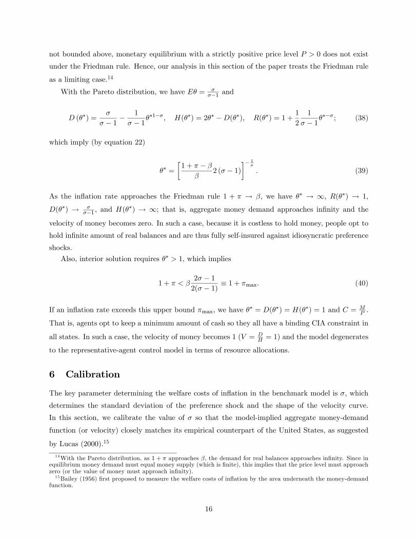
not bounded above, monetary equilibrium with a strictly positive price level P > 0 does not exist
under the Friedman rule. Hence, our analysis in this section of the paper treats the Friedman rule
as a limiting case.14
With the Pareto distribution, we have E� = ���1 and
D (��) =�
� � 1 �1
� � 1��1��; H(��) = 2�� �D(��); R(��) = 1 +
1
2
1
� � 1����; (38)
which imply (by equation 22)
�� =
�1 + � � �
�2 (� � 1)
�� 1�
: (39)
As the in�ation rate approaches the Friedman rule 1 + � ! �, we have �� ! 1, R(��) ! 1,
D(��) ! ���1 , and H(�
�) ! 1; that is, aggregate money demand approaches in�nity and the
velocity of money becomes zero. In such a case, because it is costless to hold money, people opt to
hold in�nite amount of real balances and are thus fully self-insured against idiosyncratic preference
shocks.
Also, interior solution requires �� > 1, which implies
1 + � < �2� � 12(� � 1) � 1 + �max: (40)
If an in�ation rate exceeds this upper bound �max, we have �� = D(��) = H(��) = 1 and C = MP .
That is, agents opt to keep a minimum amount of cash so they all have a binding CIA constraint in
all states. In such a case, the velocity of money becomes 1 (V = DH = 1) and the model degenerates
to the representative-agent control model in terms of resource allocations.
6 Calibration
The key parameter determining the welfare costs of in�ation in the benchmark model is �, which
determines the standard deviation of the preference shock and the shape of the velocity curve.
In this section, we calibrate the value of � so that the model-implied aggregate money-demand
function (or velocity) closely matches its empirical counterpart of the United States, as suggested
by Lucas (2000).15
14With the Pareto distribution, as 1 + � approaches �, the demand for real balances approaches in�nity. Since inequilibrium money demand must equal money supply (which is �nite), this implies that the price level must approachzero (or the value of money must approach in�nity).15Bailey (1956) �rst proposed to measure the welfare costs of in�ation by the area underneath the money-demand
function.
16

Using long-term time-series data for nominal GDP, money stock (M1), and the nominal interest
rate, Lucas (2000) showed that the ratio of M1 to nominal GDP is downward sloping against the
nominal interest rate. Lucas interpreted this downward relationship as a "money-demand" curve
and argued that it can be rationalized by the representative-agent Sidrauski (1967) model of money
in the utility:
M
PY= Ar��; (41)
where A is a scale parameter, r the nominal interest rate, and � the interest elasticity of money
demand. He showed that � = 0:5 gives the best �t.
Analogous to Lucas (2000), the money-demand curve implied by the heterogeneous-agent CIA
model of this paper takes the form
M
PY= A
H(��)
D(��); (42)
where A is a scale parameter in�uenced by the de�nition of money in the data and the cuto¤ �� is
a function of the nominal interest rate implied by equation (22). Experiments show that at annual
frequency, setting � = 1:5 and A = 0:08 provides a good �t between the model and the data.
Figure 1 plots the money-demand curves of the United States (solid circles) and that implied by
the model (solid line with cross symbols). The curve represented by the open circles is discussed
below.16
The �gure shows a good �t of the model. A key factor for the close �t of our model to the
U.S. data, in addition to the variability of the velocity of money, is the Pareto distribution for �.
The long tail property of this distribution implies that aggregate money demand (or the inverse of
velocity) can increase rapidly as in�ation approaches the Friedman rule. This property is reinforced
if the value of � is close to 1. As an example, if we set � = 3:0, then the �t is worsened signi�cantly
(see the curve represented by the open circles in Figure 1). As noted by Lucas (2000), that money
demand can rise rapidly toward in�nity near zero interest rate is important for a monetary model
to match the data.17
If the goodness of �t is measured by the metric, d = 1k
Pjm1 �m2j, where k is the number of
sample points, m1 denotes MPY based on the US data,
18 and m2 denotes the theoretical counterpart
16The circles in Figure 1 show plots of annual time series of a short-term nominal interest rate (the commercialpaper rate) against the ratio of M1 to nominal GDP for the United States for the period 1892�1997. The dataare from the online Historical Statistics of the United States�Millennium Edition. The solid line with the cross (�)symbols is the model�s prediction calibrated at annual frequency with � = 0:97; � = 0:1; � = 0:3, and � = 1:5. Thenominal interest rate in the model is de�ned as 1+�
�. The scale parameter is set to A = 0:08.
17However, Ireland (2009) shows that the more recent data from the United States do not support a steep money-demand curve near the zero interest rate. Hence, a value of � = 3 is more consistent with Ireland�s �nding based onthe more recent data.18The US data are sorted according to the nominal interest rate.
17

in the model, then the model proposed by Lucas (2000) gives d = 0:077, whereas our benchmark
model gives d = 0:059.19 Thus, the generalized heterogeneous-agent Lucas (1980) model �ts the
data better than the representative-agent Sidrauski model adopted by Lucas (2000).
Figure 1. Predicted Money Demand Curve (���) and U.S. Data (� � �).
Based on the goodness of �t for aggregate money demand, we calibrate the shape parameter
of the Pareto distribution to � = 1:5. We set the other structural parameters according to the
standard RBC literature. For example, if the time period is a year, we set � = 0:97, � = 0:1, and
� = 0:3; if the time period is a month, we set � = 0:97112 and � = 1:1
112 � 1, and so on.
7 Welfare Costs of In�ation
Following Cooley and Hansen (1989), we measure the welfare costs of in�ation by a �% increase in
compensation so that each household i is indi¤erent in terms of expected utilities between accepting
a positive in�ation � and the Friedman rule:
Z� log (1 + �) c(i; �)dF (�)�N =
Z� log ~c(i; �)dF (�)� ~N; (43)
19We set A = 0:5 in the Lucas (2000) model.
18

wheren~c(i; �); ~N
odenotes allocations under the Friedman rule. By the law of large numbers,
the expected utility of an individual is the same as the aggregate utility of all households in the
economy with equal social-welfare weights.
Given the consumption function in equation (10), the welfare cost is given by
log (1 + �) =��1��
� � 1 � logR(��) + (1� �) Y
C
�R(��)D(��)
� � 1�
� 1�: (44)
Analogously, the welfare cost of in�ation in the control model is given by
log (1 + �o) = log
�2� �
(1 + �)
�� (1� �) Y
C
�(1 + �)� �2(1 + �)� �
�: (45)
Notice that when � = �max, we have log (1 + �o) = log�
2�2��1
�� 1
2(1��)�
YC in the control model.
Figure 2. Welfare, Velocity, and Money Demand.
When the time period is a month by setting � = 0:97112 and � = 1:1
112 � 1, the welfare costs of
in�ation, the velocity of money, and the aggregate money demand implied by the heterogeneous-
agent model are depicted by the curves shown in Figure 2, where in each panel solid lines represent
19

the heterogeneous-agent model and dashed lines the control model. In the �gure, the top-left panel
shows the welfare costs of in�ation, the bottom-left panel the velocity, and the bottom-right panel
aggregate money demand. We defer discussions for the top-right panel.
Notice how heterogeneity alters the model�s implications of monetary policy. First, the top-left
panel in the �gure shows that the welfare cost curve with heterogeneous agents is astonishingly
much higher than that implied by the representative-agent model for any rate of in�ation except
near the Friedman rule. For example, when in�ation increases from 0% to 10% a year, the welfare
cost is equivalent to only 0:78% of consumption in the control model, but it is 14:6% in the
heterogeneous-agent model.
Second, the velocity of money in the heterogeneous-agent model is not constant but highly
variable with respect to in�ation. It equals zero at the Friedman-rule in�ation rate and rises
gradually with in�ation. It becomes constant at unity after the in�ation rate reaches 1 + �max =
� 2��12(��1) = 1:994 9. That is, the velocity of money reaches its upper bound of 1 after the in�ation
rate becomes 200% per month � in which case the CIA constraint binds for all agents in all states
of nature because holding money becomes too costly. At this point, the precautionary motive of
money demand disappears completely and the model becomes identical to the control model in
terms of aggregate allocations.
Third, the aggregate money demand in the heterogeneous-agent model is far larger and more
in�ation elastic than that in the control model. In particular, near the Friedman rule, aggregate
demand for real balances in the heterogeneous-agent model is arbitrarily close to in�nity; but, as
in�ation rises, demand for real balances drops rapidly and converge from above to that in the
control model. The excessively large aggregate demand for money in the heterogeneous-agent
model at low in�ation rates arises because of a strong precautionary motive for holding cash to
bu¤er idiosyncratic preference shocks. However, when the in�ation rate increases, such an incentive
for self-insurance diminishes. In contrast, money demand declines very slowly with in�ation in the
control model. Such a di¤erence in the behavior of money demand implies a large discrepancy of the
welfare cost of in�ation between the two models for two reasons: (i) The precautionary insurance
motive induces agents to hold an excessively large amount of cash at low in�ation rates; which
raises the welfare cost of in�ation due to a larger base for the in�ation tax (the Bailey triangle).
(ii) More importantly, in�ation destroys the liquidity value of money and raises the portion of the
cash-constrained population by reducing the incentives of holding money; when households become
cash-constrained, they are not able to raise consumption according to the marginal utility.
To see how the representative-agent assumption seriously distorts the estimates of the welfare
costs of in�ation, consider an alternative (but incorrect) measure of the welfare cost of in�ation in
the heterogeneous-agent model, which is to use the average consumption C =Rc(i)di to measure
20

social welfare:
�� log
��1 + ��
� Zc(i)di
��N = �� log
�Z~c(i)di
�� ~N: (46)
This implies
log�1 + ��
�= log
�
1 + ��log
1� 1
�
�1 + � � �
�2 (� � 1)
���1�
!+(1� �) Y
C
�R(��)D(��)
� � 1�
� 1�:
(47)
With this alternative measure, if � = �max, then log�1 + ��
�= log
�2�2��1
�� 1
2(1��)�
YC , which is
identical to that in the control model. In fact, at both the Friedman-rule in�ation rate and for
in�ation rates � � �max, the aggregate allocation of the heterogeneous-agent model is identical
to that of the control model; hence, the welfare implications are also identical in those ranges
of in�ation rates if we use the utility of average consumption (instead of the average utility of
individual consumption) as the base to measure welfare.
The top-right panel in Figure 2 shows that the alternative measure of welfare in equation (47)
is far closer to that of the control model, and it di¤ers from the control model only moderately
in the in�ation range � 2 (� � 1; �max). This incorrect measure coincides with that of the controlmodel for high in�ation rates because all households are liquidity constrained when � � �max andthis measure ignores the idiosyncratic risk facing individual agents when they become liquidity
constrained. That is, from the point of view of average consumption, it does not matter whether or
not individuals are self-insured. In contrast, with the correct welfare measure that takes into account
individual risk, the costs of in�ation are dramatically di¤erent between the two economies even when
in�ation is su¢ ciently high (i.e., � � �max) so that all agents become liquidity-constrained.Why does heterogeneity matter so much for welfare costs? The crucial reason is that, with
low in�ation, the CIA constraint does not bind for most agents (or not very often for the same
agent) because of precautionary saving motives under idiosyncratic risk. This is very di¤erent from
representative-agent models where the CIA constraint always binds under aggregate risks. This
implies a larger welfare gain from reducing in�ation toward the Friedman rule in the heterogeneous-
agent model than in the control model.
Figure 3 plots the probability of a binding CIA constraint in the heterogeneous-agent model
as a function of the in�ation rate. It shows that the probability of liquidity constraint is very low
under moderate in�ation, suggesting that most agents are very well self-insured most of the time.
However, as in�ation increases, the probability of a binding CIA constraint rises rapidly, thus more
agents (especially those with the most urge to consume) will become liquidity-constrained, which
reduces social welfare signi�cantly along the extensive margin because self-insurance can provide
21

far larger welfare than a low in�ation tax could � namely, the opportunity cost of holding non-
interest�bearing cash (the Bailey triangle) is relatively less important compared with the loss of
self-insurance as in�ation increases.
Figure 3. Probability of a Binding CIA Constraint.
Notice in Figure 3 the probability of a binding borrowing constraint is a linear function of the
in�ation rate. A formal proof of this result is provided here. Equation (22) implies 1+�� = R(��) =
1 + 12
1��1�
���, which implies ���� = 2 (� � 1) 1+���� . Hence, 1 � F (��) is a linear function of
in�ation. Suppose � = 0:97 and � = 0:1; then 1 � F (��) = 13:4%. That is, when the time periodis a year and the annual in�ation rate is 10%, households still opt to hold so much money that the
probability of a binding CIA constraint is less than 14%. This result is in sharp contrast to that
obtained by Hodrick, Kocherlakota, and Lucas (1991) based on a representative-agent CIA model,
where they show that the probability of a binding CIA constraint is close to 100% regardless of the
in�ation rate.
In other words, although precautionary demand for money will raise the in�ation tax on house-
holds, the more important contributing factor to the large welfare cost of in�ation is the inability to
self-insure when the CIA constraint binds. With idiosyncratic risk, the Friedman rule ensures that
agents are fully insured against such shocks so that consumption comoves perfectly with preference
shocks (�). When in�ation rises, the probability of a binding CIA constraint increases because of
lower money demand, which implies that the portion of CIA-constrained agents also increases. Since
the welfare of a liquidity-constrained agent is signi�cantly lower than that of a cash-rich agent be-
22

cause of the lack of self-insurance, in�ation� by making more agents liquidity-constrained� is very
costly. This adverse liquidity e¤ect along the extensive margin is also noted by Imrohoroglu (1992)
and Wen (2009) based on a Bewley (1980) model.
As the variance of idiosyncratic risk diminishes, the heterogeneous-agent model gradually re-
duces to a representative-agent model. The example shown in Figure 4 is generated under the
same parameter values as before but a signi�cantly smaller variance of � by setting � = 30. The
�gure shows that the heterogeneous-agent model converges to the representative-agent counterpart.
In particular, the velocity of money in the heterogeneous-agent model approaches unity almost as
soon as the in�ation rate departs from the Friedman rule (see the lower-left panel), and aggregate
money demand in the two models becomes virtually identical when the monthly in�ation rate � is
as low as 1:014 (see the lower-right panel). Most notably, the gap in the welfare costs of in�ation
between the two models is no longer so dramatic (albeit still signi�cant, see the upper-left panel),
and the welfare measure based on average consumption becomes virtually identical to that in the
representative-agent model for all in�ation rates (see the upper-right panel).
Figure 4. Welfare, Velocity, and Money Demand (� = 30).
Table 1 provides sensitivity analyses of the welfare costs to di¤erent calibrations when the
annualized in�ation rate increases from 0% to 10%. The table shows that the welfare costs are
23
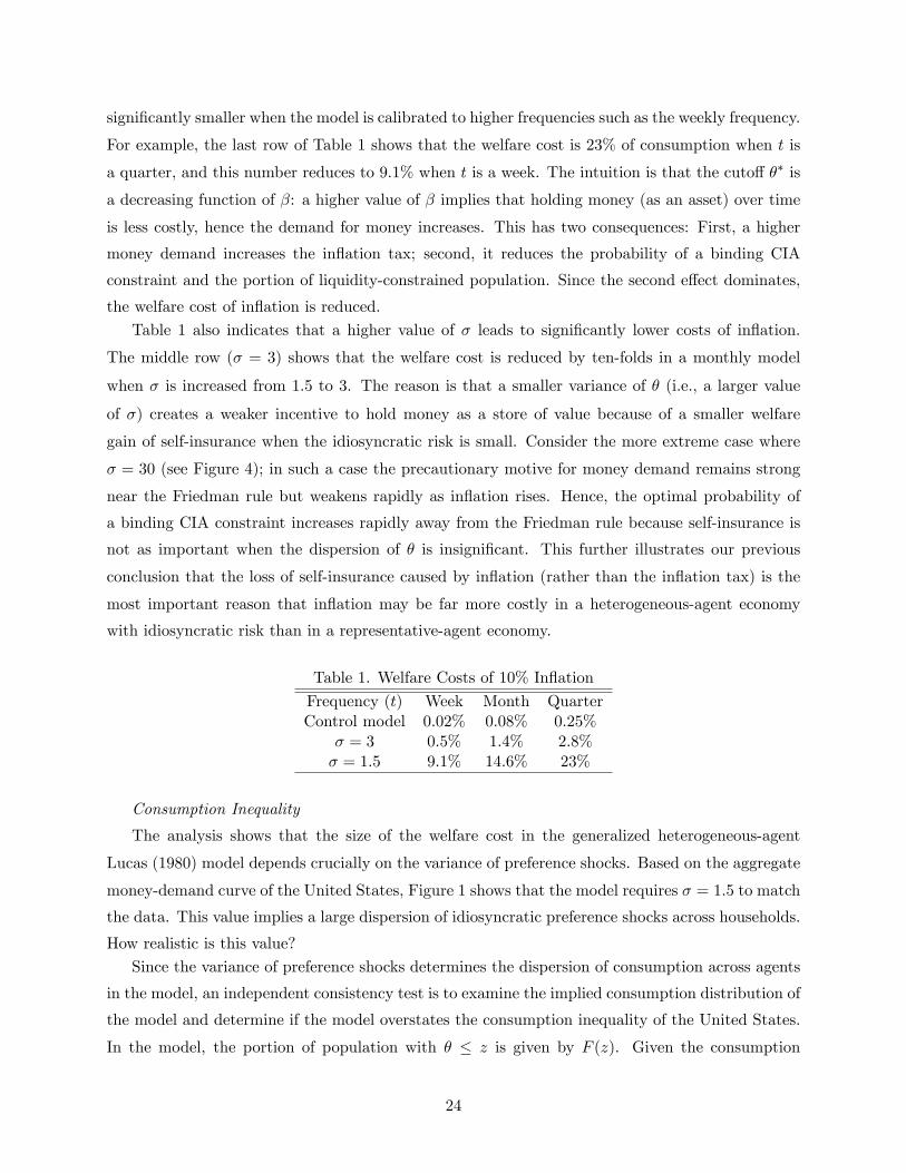
signi�cantly smaller when the model is calibrated to higher frequencies such as the weekly frequency.
For example, the last row of Table 1 shows that the welfare cost is 23% of consumption when t is
a quarter, and this number reduces to 9:1% when t is a week. The intuition is that the cuto¤ �� is
a decreasing function of �: a higher value of � implies that holding money (as an asset) over time
is less costly, hence the demand for money increases. This has two consequences: First, a higher
money demand increases the in�ation tax; second, it reduces the probability of a binding CIA
constraint and the portion of liquidity-constrained population. Since the second e¤ect dominates,
the welfare cost of in�ation is reduced.
Table 1 also indicates that a higher value of � leads to signi�cantly lower costs of in�ation.
The middle row (� = 3) shows that the welfare cost is reduced by ten-folds in a monthly model
when � is increased from 1:5 to 3. The reason is that a smaller variance of � (i.e., a larger value
of �) creates a weaker incentive to hold money as a store of value because of a smaller welfare
gain of self-insurance when the idiosyncratic risk is small. Consider the more extreme case where
� = 30 (see Figure 4); in such a case the precautionary motive for money demand remains strong
near the Friedman rule but weakens rapidly as in�ation rises. Hence, the optimal probability of
a binding CIA constraint increases rapidly away from the Friedman rule because self-insurance is
not as important when the dispersion of � is insigni�cant. This further illustrates our previous
conclusion that the loss of self-insurance caused by in�ation (rather than the in�ation tax) is the
most important reason that in�ation may be far more costly in a heterogeneous-agent economy
with idiosyncratic risk than in a representative-agent economy.
Table 1. Welfare Costs of 10% In�ation
Frequency (t) Week Month QuarterControl model 0.02% 0.08% 0.25%
� = 3 0.5% 1.4% 2.8%� = 1:5 9.1% 14.6% 23%
Consumption Inequality
The analysis shows that the size of the welfare cost in the generalized heterogeneous-agent
Lucas (1980) model depends crucially on the variance of preference shocks. Based on the aggregate
money-demand curve of the United States, Figure 1 shows that the model requires � = 1:5 to match
the data. This value implies a large dispersion of idiosyncratic preference shocks across households.
How realistic is this value?
Since the variance of preference shocks determines the dispersion of consumption across agents
in the model, an independent consistency test is to examine the implied consumption distribution of
the model and determine if the model overstates the consumption inequality of the United States.
In the model, the portion of population with � � z is given by F (z). Given the consumption
24
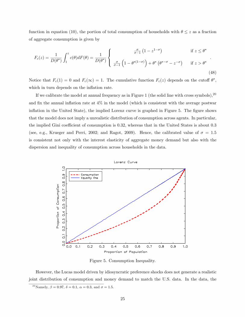
function in equation (10), the portion of total consumption of households with � � z as a fractionof aggregate consumption is given by
Fc(z) =1
D(��)
Z z
1c(�)dF (�) =
1
D(��)
8><>:���1
�1� z1��
�if z � ��
���1
�1� ��(1��)
�+ ��
����� � z��
�if z > ��
:
(48)
Notice that Fc(1) = 0 and Fc(1) = 1. The cumulative function Fc(z) depends on the cuto¤ ��,
which in turn depends on the in�ation rate.
If we calibrate the model at annual frequency as in Figure 1 (the solid line with cross symbols),20
and �x the annual in�ation rate at 4% in the model (which is consistent with the average postwar
in�ation in the United State), the implied Lorenz curve is graphed in Figure 5. The �gure shows
that the model does not imply a unrealistic distribution of consumption across agents. In particular,
the implied Gini coe¢ cient of consumption is 0:32, whereas that in the United States is about 0:3
(see, e.g., Krueger and Perri, 2002; and Ragot, 2009). Hence, the calibrated value of � = 1:5
is consistent not only with the interest elasticity of aggregate money demand but also with the
dispersion and inequality of consumption across households in the data.
Figure 5. Consumption Inequality.
However, the Lucas model driven by idiosyncratic preference shocks does not generate a realistic
joint distribution of consumption and money demand to match the U.S. data. In the data, the20Namely, � = 0:97, � = 0:1, � = 0:3, and � = 1:5.
25
distribution of consumption is positively correlated with that of money demand (see, e.g., Ragot,
2009). This implies that households with low consumption also hold less cash in the data. But with
i.i.d. preference shocks, households with the least urge to consume will carry the largest amount
of money in the model, which implies a negative correlation between consumption distribution and
cash distribution. This counterfactual joint distribution of consumption and money demand does
not exist in the model of Wen (2009) in which the source of idiosyncratic risk comes from wealth.
It is therefore expected that introducing wealth shocks or highly persistent preference shocks into
the Lucas model may resolve this problem.21
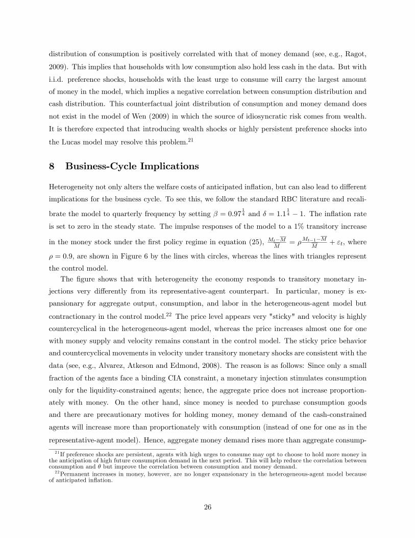
8 Business-Cycle Implications
Heterogeneity not only alters the welfare costs of anticipated in�ation, but can also lead to di¤erent
implications for the business cycle. To see this, we follow the standard RBC literature and recali-
brate the model to quarterly frequency by setting � = 0:9714 and � = 1:1
14 � 1. The in�ation rate
is set to zero in the steady state. The impulse responses of the model to a 1% transitory increase
in the money stock under the �rst policy regime in equation (25), Mt�MM
= �Mt�1�MM
+ "t, where
� = 0:9, are shown in Figure 6 by the lines with circles, whereas the lines with triangles represent
the control model.
The �gure shows that with heterogeneity the economy responds to transitory monetary in-
jections very di¤erently from its representative-agent counterpart. In particular, money is ex-
pansionary for aggregate output, consumption, and labor in the heterogeneous-agent model but
contractionary in the control model.22 The price level appears very "sticky" and velocity is highly
countercyclical in the heterogeneous-agent model, whereas the price increases almost one for one
with money supply and velocity remains constant in the control model. The sticky price behavior
and countercyclical movements in velocity under transitory monetary shocks are consistent with the
data (see, e.g., Alvarez, Atkeson and Edmond, 2008). The reason is as follows: Since only a small
fraction of the agents face a binding CIA constraint, a monetary injection stimulates consumption
only for the liquidity-constrained agents; hence, the aggregate price does not increase proportion-
ately with money. On the other hand, since money is needed to purchase consumption goods
and there are precautionary motives for holding money, money demand of the cash-constrained
agents will increase more than proportionately with consumption (instead of one for one as in the
representative-agent model). Hence, aggregate money demand rises more than aggregate consump-
21 If preference shocks are persistent, agents with high urges to consume may opt to choose to hold more money inthe anticipation of high future consumption demand in the next period. This will help reduce the correlation betweenconsumption and � but improve the correlation between consumption and money demand.22Permanent increases in money, however, are no longer expansionary in the heterogeneous-agent model because
of anticipated in�ation.
26
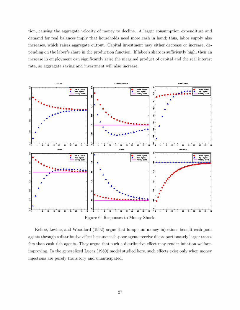
tion, causing the aggregate velocity of money to decline. A larger consumption expenditure and
demand for real balances imply that households need more cash in hand; thus, labor supply also
increases, which raises aggregate output. Capital investment may either decrease or increase, de-
pending on the labor�s share in the production function. If labor�s share is su¢ ciently high, then an
increase in employment can signi�cantly raise the marginal product of capital and the real interest
rate, so aggregate saving and investment will also increase.
Figure 6. Responses to Money Shock.
Kehoe, Levine, and Woodford (1992) argue that lump-sum money injections bene�t cash-poor
agents through a distributive e¤ect because cash-poor agents receive disproportionately larger trans-
fers than cash-rich agents. They argue that such a distributive e¤ect may render in�ation welfare-
improving. In the generalized Lucas (1980) model studied here, such e¤ects exist only when money
injections are purely transitory and unanticipated.
27

9 Conclusion
This paper provides an analytically tractable general-equilibrium version of the Lucas (1980) model.
The model makes predictions about monetary business cycle and the welfare costs of in�ation that
are quite di¤erent from those of the representative-agent literature. For example, (i) the velocity of
money is signi�cantly variable in a heterogeneous-agent CIA model, in contrast to the �ndings of
Hodrick, Kocherlakota, and Lucas (1991) based on a representative-agent CIA framework; (ii)
transitory lump-sum monetary injections have expansionary e¤ects on aggregate consumption,
employment, and output despite �exible prices, unlike the implications of the representative-agent
assumption; and (iii) anticipated in�ation can be potentially far more costly than indicated by the
literature: with a su¢ ciently strong precautionary motive for cash holdings to match the interest
elasticity of aggregate money demand and consumption inequality in the United States, households
are willing to give up 10% to 15% of consumption to avoid 10% annual in�ation. This number is
also several times larger than implied by the LW (2005) model.
The �rst two �ndings are comparable to those in the Baumol-Tobin model (e.g., Alvarez, Atke-
son, Edmond, 2009; Rotermberg, 1984; and others). The third �nding, to the best of my knowledge,
has not been shown within the Baumol-Tobin framework. The large welfare cost of in�ation arises
because (i) the precautionary insurance motive induces agents to hold an excessively large amount
of cash, which raises the welfare cost of in�ation due to an increased opportunity cost for holding
non-interest�bearing assets; (ii) more importantly, in�ation destroys the liquidity value of money
and renders an increasingly larger fraction of the population without self-insurance. Such e¤ects
and mechanisms are not captured by representative-agent CIA models (e.g., Cooley and Hansen,
1989).23
The ability to obtain closed-form solutions for the distribution of money demand is an additional
contribution of this paper. The analytical intractability of the original Lucas (1980) model has
limited its applicability and hence induced researchers (i) to use representative versions of that
model for policy analysis or (ii) to rely almost exclusively on the Baumol-Tobin framework to study
the issue of heterogeneous money demand and the associated policy implications. Hopefully, the
analysis here may convince readers that the Lucas (1980) model can serve as a fruitful alternative
to the Baumol-Tobin framework for optimal money demand and policy analysis.
23Wen (2009) obtain similar welfare results using a generalized Bewley (1980) model.
28

Appendix: Proof of Proposition 1
Proof. The decision rules at the individual level are characterized by a cuto¤ strategy. We assume
an interior solution for hours worked and use a guess-and-verify strategy to derive the decision rules
of individuals. The key to the analysis is to show that the cuto¤ is independent of i in each period.
In anticipation of this result, we denote the cuto¤ by ��t without the index i. Consider two possiblecases:
Case A: �t(i) � ��t . In this case, the urge to consume is low. Hence, it is optimal not to
spend all cash in hand to buy consumption goods but carry the excess money as inventories for
the future. Thus, ct(i) � mt(i)Pt, vt(i) = 0, and equation (8) implies the shadow value of good
�t(i) = �EtPt
Wt+1Pt+1. Equation (4) implies ct(i) = �t(i)
��Et
PtPt+1Wt+1
��1. Using the de�nition in
equation (1), the budget identity (2) then implies
mt(i)
Pt= xt(i)� �t(i)
��Et
PtPt+1Wt+1
��1: (49)
The requirement mt(i)Pt
� ct(i) then implies xt(i) � 2�t(i)��Et
PtPt+1Wt+1
��1, or
�t(i) �1
2xt(i)�Et
PtPt+1Wt+1
� ��t ; (50)
which de�nes the cuto¤ ��t . This de�nition of ��t implies
xt(i) = 2��t
��Et
PtPt+1Wt+1
��1: (51)
Hence, we have mt(i)Pt
= (2��t��t(i))2��t
xt(i) and ct(i) = 12�t(i)��txt(i), which together imply ct(i) =
�t(i)2��t��t(i)
mt(i)Pt
� mt(i)Pt.
Case B: �t(i) > ��t . In this case the urge to consume is high. It is then optimal to spend all
cash in hand for consumption, so vt(i) > 0 and ct(i) =mt(i)Pt. By the resource constraint (2), we
have ct(i) = 12xt(i), which by equation (51) implies ct(i) = �
�t
��Et
PtPt+1Wt+1
��1. Equations (4) and
(6) then imply vt(i) =�t(i)��t�Et
PtPt+1Wt+1
� �t(i) =��t(i)��t
� 1��Et
PtPt+1Wt+1
� vt(i), which gives
vt(i) =1
2
��t(i)
��t� 1��Et
PtPt+1Wt+1
> 0. (52)
29

Hence, the shadow value of goods is given by
�t(i) =1
2
��t(i)
��t+ 1
��Et
PtPt+1Wt+1
: (53)
Notice that the shadow price �t(i) is higher under Case B than under Case A.
The above analyses imply that the shadow price �t(i) takes two possible values associated with
Case A and Case B, respectively. Hence, the expected shadow value of goods, ~E�t(i), can be
explicitly solved. Consequently, equation (5) becomes
1
Wt= �Et
PtPt+1Wt+1
R(��t ); (54)
where
R(��t ) �"Z
�t(i)���tdF (�) +
Z�t(i)>�
�t
1
2
��t(i)
��t+ 1
�dF (�)
#: (55)
Equation (54) is equation (13) in Proposition 1. Equations (54) and (55) imply that the cuto¤ ��t
is independent of i under the assumption that �(i) is i.i.d. Equation (50) then implies that the
optimal cash in hand, xt(i), is also independent of i. Using equation (54), based on case A and
case B, the decision rules of household i�s consumption, money holdings, and cash in hand are then
summarized by equations (10)-(12), respectively.
30

References
[1] Aiyagari, R., 1994, Uninsured idiosyncratic risk and aggregate saving, Quarterly Journal of
Economics 109(3), 659-84.
[2] Akyol, A., 2004, Optimal monetary policy in an economy with incomplete markets and idio-
syncratic risk, Journal of Monetary Economics 51(6), 1245-1269.
[3] Algan, X. Ragot, 2010...
[4] Alvarez, F., A. Atkeson and C. Edmond, 2009, Sluggish responses of prices and in�ation to
monetary shocks in an inventory model of money demand, Quarterly Journal of Economics
124(3), 911-967.
[5] Alvarez, F., A. Atkeson and P. Kehoe, 1999, Money and interest rates with endogenously
segmented markets, NBER Working Paper No. w7060.
[6] Aruoba, B., C. Waller, and R. Wright, 2009, Money and capital: A quantitative analysis,
Federal Reserve Bank of St. Louis Working Paper 2009-031A.
[7] Aruoba, B. and R. Wright, 2003, Search, money and capital: A neoclassical dichotomy, Journal
of Money, Credit and Banking 35, 1086-1105.
[8] Bailey, M., 1956, The welfare cost of in�ationary �nance, Journal of Political Economy 64,
93-110.
[9] Baumol, William J., 1952, The Transactions Demand for Cash: An Inventory Theoretic Ap-
proach, Quarterly Journal of Economics 66(4), 545-556.
[10] Bewley, T., 1980, "The Optimum Quantity of Money," in Models of Monetary Economics, ed.
by John Kareken and Neil Wallace. Minneapolis, Minnesota: Federal Reserve Bank, 1980.
[11] Blanchard, Olivier J. and Charles M. Kahn, 1980, The solution of linear di¤erence models
under rational expectations, Econometrica 48(5), 1305-1311.
[12] Boel, P. and G. Camera, 2009, Financial sophistication and the distribution of the welfare cost
of in�ation, Journal of Monetary Economics 56, 968�978.
[13] Chatterjee, S. and D. Corbae, 1992, Endogenous market participation and the general equi-
librium value of money, The Journal of Political Economy 100(3), 615-646.
[14] Chiu, J., 2007, Endogenously segmented asset market in an inventory theoretic model of money
demand, Bank of Canada Working Paper 2007-46.
31

[15] Cooley, T. and G. Hansen, 1989, The in�ation tax in a real business cycle model, American
Economic Review 79(4), 733-748.
[16] Costa, C and I. Werning, 2008, On the optimality of the Friedman rule with heterogeneous
agents and nonlinear income taxation, Journal of Political Economy 116(1), 82-112.
[17] Dotsey, M. and P. Ireland, 1996, The welfare cost of in�ation in general equilibrium, Journal
of Monetary Economics 37(1), 29-47.
[18] Erosa, A., and Ventura, G., 2002, On in�ation as a regressive consumption tax, Journal of
Monetary Economics 49, 761�795.
[19] Grossman, S. and L. Weiss, 1983, A transactions-based model of the monetary transmission
mechanism, American Economic Review 73(5), 871-80.
[20] Heathcote, J., K. Storesletten and G. Violante, 2008, Quantitative macroeconomics with het-
erogeneous households, Federal Reserve Bank of Minneapolis Research Department Sta¤ Re-
port 420 (September).
[21] Helpman, E., 1981, An exploration in the theory of exchange rate regimes, Journal of Political
Economy 89, 865-890.
[22] Hodrick, R., N., Kocherlakota, and D. Lucas, 1991, The variability of velocity in cash-in-
advance models, Journal of Political Economy 99(2), 358-384.
[23] Huggett, M., 1993, The risk-free rate in heterogeneous-agent incomplete-insurance economies,
Journal of Economic Dynamics and Control 17(5-6), 953-969.
[24] Huggett, M., 1997, The one-sector growth model with idiosyncratic shocks: Steady states and
dynamics, Journal of Monetary Economics 39(3), 385-403.
[25] Imrohoroglu, A., 1989, Cost of business cycles with indivisibilities and liquidity constraints,
Journal of Political Economy 97(6), 1364-1383.
[26] Imrohoroglu, A., 1992, The welfare cost of in�ation under imperfect insurance, Journal of
Economic Dynamics and Control 16(1), 79-91.
[27] Ireland, P., 1996, The role of countercyclical monetary policy, The Journal of Political Economy
104(4), 704-723.
[28] Ireland, P., 2009, On the welfare cost of in�ation and the recent behavior of money demand,
American Economic Review 99(3), 1040-1052.
32

[29] Jellou, M.B., 2007, Money, self insurance and liquidity: Baumol and Tobin meet Bewley, Paris
School of Economics Working Paper.
[30] Jovanovic, B., 1982, In�ation and welfare in the steady state, Journal of Political Economy
90, 561-577.
[31] Kehoe, T., D. Levine, and M. Woodford, 1992, The optimum quantity of money revisited,
in Economic Analysis of Markets and Games, ed. by P. Dasgupta, D. Gale, 0. Hart, and E.
Maskin, Cambridge, Mass.: M.I.T. Press.
[32] Khan, A. and J. Thomas, 2007, In�ation and Interest Rates with Endogenous Market Seg-
mentation, Federal Reserve Bank of Philadelphia working paper.
[33] King, R., C. Plosser and S. Rebelo, 1988, Production, growth, and business cycles: I. The
basic neoclassical model, Journal of Monetary Economics 21(2-3), 195-232.
[34] Krusell, P. and A. Smith, Jr., 1998, Income and Wealth Heterogeneity in the Macroeconomy,
Journal of Political Economy 106(5), 867-895.
[35] Krusell, P. and A. Smith, 1999, On the welfare e¤ects of eliminating business cycles, Review
of Economic Dynamics 2(1), 245-72.
[36] Lagos, R. and R. Wright, 2005, A Uni�ed Framework for Monetary Theory and Policy Analysis,
Journal of Political Economy 113(3), 463-484.
[37] Levine, D. and W. Zame, 2002, Does market incompleteness matter? Econometrica 70(5),
1805-1839.
[38] Lucas, R.E. Jr., 1980, Equilibrium in a Pure Currency Economy, Economic Inquiry 18(2),
203-220.
[39] Lucas, R.E. Jr., 1984, Money in a Theory of Finance, Carnegie-Rochester Conference Series
for Public Policy 21, 9-45.
[40] Lucas, R.E. Jr., 2000, In�ation and welfare, Econometrica, Vol. 68(2), 247-274.
[41] Lucas, R.E. Jr. and N. Stokey, 1987, Money and interest in a cash-in-advance economy, Econo-
metrica 55(3), 491-513.
[42] Ragot, X., 2009, The case for a �nancial approach to money demand, Working Paper, Banque
de France.
33
[43] Romer, D., 1986, A simple general equilibrium version of the Baumol-Tobin model. The Quar-
terly Journal of Economics, 101(4):663 686.
[44] Rotermberg, J., 1984, A monetary equilibrium model with transactions costs. Journal of Po-
litical Economy 92(1), 4-58.
[45] Sidrauski, M, 1967, �Rational Choice and Patterns of Growth in a Monetary Econ-
omy,�American Economic Review, 57(2), 534 544.
[46] Stokey, N. and R. Lucas (with E. Prescott), 1989, Recursive Methods in Economic Dynamics,
Cambridge, Mass.: Harvard University Press.
[47] Svensson, Lars, E.O., 1985, Money and asset prices in a cash-in-advance economy, Journal of
Political Economy, 93(5), 919-944.
[48] Telyukova, I. and L. Visschers, 2009, Precautionary demand for money in a monetary business
cycle model, Working Paper.
[49] Tobin, J., 1956, The interest-elasticity of the transactions demand for cash, Review of Eco-
nomics and Statistics. 38(3), 241-247.
[50] Wen, Y., 2008, Input and output inventory dynamics, Federal Reserve Bank of St. Louis
Working Paper 2008-008B.
[51] Wen, Y., 2009, Liquidity demand and welfare in a heterogeneous-agent economy, Federal
Reserve Bank of St. Louis Working Paper 2010-009A.
[52] Yaari, M., 1976, A law of large numbers in the theory of consumer�s choice under uncertainty,
Journal of Economic Theory, 12, 202-217.
34
Recommended