Sri Vidya College of Engineering & Technology, Virudhunagar Course Material (Lecture Notes)
IT 6501 & Graphics and Multimedia Unit 2 Page 1
LP 1: Three Dimensional Object Representations
Representation schemes for solid objects are divided into two categories as follows:
1. Boundary Representation ( B-reps)
It describes a three dimensional object as a set of surfaces that separate the object interior from
the environment. Examples are polygon facets and spline patches.
2. Space Partitioning representation
It describes the interior properties, by partitioning the spatial region containing an object into a
set of small, nonoverlapping, contiguous solids(usually cubes). Eg: Octree Representation.
Polygon Surfaces
Polygon surfaces are boundary representations for a 3D graphics object is a set of polygons that
enclose the object interior.
Polygon Tables
The polygon surface is specified with a set of vertex coordinates and associated attribute
parameters.
For each polygon input, the data are placed into tables that are to be used in the subsequent
processing.
Polygon data tables can be organized into two groups: Geometric tables and attribute
tables.
Geometric Tables Contain vertex coordinates and parameters to identify the spatial orientation
of the polygon surfaces.
Attribute tables Contain attribute information for an object such as parameters specifying the
degree of transparency of the object and its surface reflectivity and texture characteristics. A
convenient organization for storing geometric data is to create three lists:
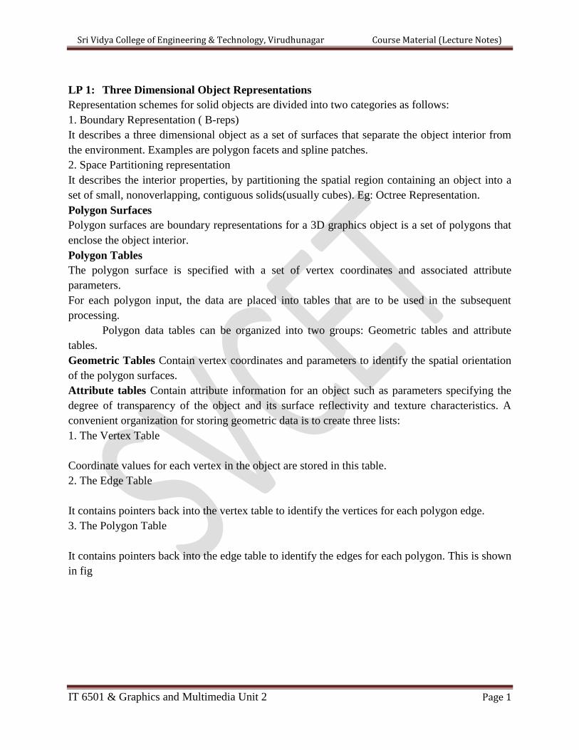
1. The Vertex Table
Coordinate values for each vertex in the object are stored in this table.
2. The Edge Table
It contains pointers back into the vertex table to identify the vertices for each polygon edge.
3. The Polygon Table
It contains pointers back into the edge table to identify the edges for each polygon. This is shown
in fig
Sri Vidya College of Engineering & Technology, Virudhunagar Course Material (Lecture Notes)
IT 6501 & Graphics and Multimedia Unit 2 Page 2
Listing the geometric data in three tables provides a convenient reference to the individual
components (vertices, edges and polygons) of each object.
The object can be displayed efficiently by using data from the edge table to draw the component
lines.
Extra information can be added to the data tables for faster information extraction. For instance,
edge table can be expanded to include forward points into the polygon table so that common
edges between polygons can be identified more rapidly.
E1 : V1, V2, S1
E2 : V2, V3, S1
E3 : V3, V1, S1, S2
E4 : V3, V4, S2
E5 : V4, V5, S2
E6 : V5, V1, S2
is useful for the rendering procedure that must vary surface shading smoothly across the edges
from one polygon to the next. Similarly, the vertex table can be expanded so that vertices are
cross-referenced to corresponding edges.
Additional geometric information that is stored in the data tables includes the slope for each edge
and the coordinate extends for each polygon. As vertices are input, we can calculate edge slopes
and we can scan the coordinate values to identify the minimum and maximum x, y and z values
for individual polygons.
Sri Vidya College of Engineering & Technology, Virudhunagar Course Material (Lecture Notes)
IT 6501 & Graphics and Multimedia Unit 2 Page 3
The more information included in the data tables will be easier to check for errors.
Some of the tests that could be performed by a graphics package are:
1. That every vertex is listed as an endpoint for at least two edges.
2. That every edge is part of at least one polygon.
3. That every polygon is closed.
4. That each polygon has at least one shared edge.
5. That if the edge table contains pointers to polygons, every edge referenced by a polygon
pointer has a reciprocal pointer back to the polygon.
Plane Equations:
To produce a display of a 3D object, we must process the input data representation for the object
through several procedures such as,
- Transformation of the modeling and world coordinate descriptions to viewing coordinates.
- Then to device coordinates:
- Identification of visible surfaces
- The application of surface-rendering procedures.
For these processes, we need information about the spatial orientation of the individual surface
components of the object. This information is obtained from the vertex coordinate value and the
equations that describe the polygon planes.
The equation for a plane surface is
Ax + By+ Cz + D = 0 ----(1)
Where (x, y, z) is any point on the plane, and the coefficients A,B,C and D are constants
describing the spatial properties of the plane.
We can obtain the values of A, B,C and D by solving a set of three plane equations using the
coordinate values for three non collinear points in the plane.
For that, we can select three successive polygon vertices (x1, y1, z1), (x2, y2, z2) and (x3, y3,
z3) and solve the following set of simultaneous linear plane equations for the ratios A/D, B/D
and C/D.
(A/D)xk + (B/D)yk + (c/D)zk = -1, k=1,2,3 -----(2)
The solution for this set of equations can be obtained in determinant form, using Cramer’s rule as
1 y1 z1 x1 1 z1 x1 y1 1 x1 y1 z1
A= 1 y2 z2 B= x2 1 z2 C= x2 y2 1 D= x2 y2 z2 ----(3)
1 y3 z3 x3 1 z3 x3 y3 1 x3 y3 z3
Expanding the determinants , we can write the calculations for the plane coefficients in the form:
A = y1 (z2 –z3 ) + y2(z3 –z1 ) + y3 (z1 –z2 )
B = z1 (x2 -x3 ) + z2 (x3 -x1 ) + z3 (x1 -x2 )
Sri Vidya College of Engineering & Technology, Virudhunagar Course Material (Lecture Notes)
IT 6501 & Graphics and Multimedia Unit 2 Page 4
C = x1 (y2 –y3 ) + x2 (y3 –y1 ) + x3 (y1 -y2 )
D = -x1 (y2 z3 -y3 z2 ) - x2 (y3 z1 -y1 z3 ) - x3 (y1 z2 -y2 z1) ------(4)
As vertex values and other information are entered into the polygon data structure, values for A,
B, C and D are computed for each polygon and stored with the other polygon data.
Plane equations are used also to identify the position of spatial points relative to the plane
surfaces of an object. For any point (x, y, z) hot on a plane with parameters A,B,C,D, we have
Ax + By + Cz + D ≠ 0
We can identify the point as either inside or outside the plane surface according o the sigh
(negative or positive) of Ax + By + Cz + D:
If Ax + By + Cz + D < 0, the point (x, y, z) is inside the surface. If Ax + By + Cz + D > 0, the
point (x, y, z) is outside the surface.
These inequality tests are valid in a right handed Cartesian system, provided the plane parmeters
A,B,C and D were calculated using vertices selected in a counter clockwise order when viewing
the surface in an outside-to-inside direction.
Polygon Meshes
A single plane surface can be specified with a function such as fillArea. But when object
surfaces are to be tiled, it is more convenient to specify the surface facets with a mesh function.
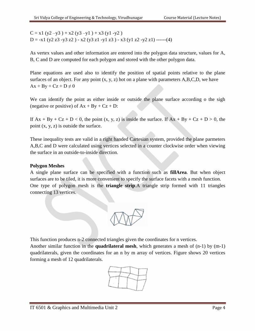
One type of polygon mesh is the triangle strip.A triangle strip formed with 11 triangles
connecting 13 vertices.
This function produces n-2 connected triangles given the coordinates for n vertices.
Another similar function in the quadrilateral mesh, which generates a mesh of (n-1) by (m-1)
quadrilaterals, given the coordinates for an n by m array of vertices. Figure shows 20 vertices
forming a mesh of 12 quadrilaterals.
Sri Vidya College of Engineering & Technology, Virudhunagar Course Material (Lecture Notes)
IT 6501 & Graphics and Multimedia Unit 2 Page 5
Curved Lines and Surfaces Displays of three dimensional curved lines and surface can be
generated from an input set of mathematical functions defining the objects or from a set of user
specified data points. When functions are specified, a package can project the defining equations
for a curve to the display plane and plot pixel positions along the path of the projected function.
For surfaces, a functional description in decorated to produce a polygon-mesh approximation to
the surface.
Spline Representations A Spline is a flexible strip used to produce a smooth curve through a
designated set of points. Several small weights are distributed along the length of the strip to
hold it in position on the drafting table as the curve is drawn.
The Spline curve refers to any sections curve formed with polynomial sections satisfying
specified continuity conditions at the boundary of the pieces.
A Spline surface can be described with two sets of orthogonal spline curves. Splines are used in
graphics applications to design curve and surface shapes, to digitize drawings for computer
storage, and to specify animation paths for the objects or the camera in the scene. CAD
applications for splines include the design of automobiles bodies, aircraft and spacecraft
surfaces, and ship hulls.
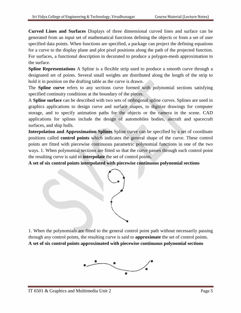
Interpolation and Approximation Splines Spline curve can be specified by a set of coordinate
positions called control points which indicates the general shape of the curve. These control
points are fitted with piecewise continuous parametric polynomial functions in one of the two
ways. 1. When polynomial sections are fitted so that the curve passes through each control point
the resulting curve is said to interpolate the set of control points.
A set of six control points interpolated with piecewise continuous polynomial sections
1. When the polynomials are fitted to the general control point path without necessarily passing
through any control points, the resulting curve is said to approximate the set of control points.
A set of six control points approximated with piecewise continuous polynomial sections
Sri Vidya College of Engineering & Technology, Virudhunagar Course Material (Lecture Notes)
IT 6501 & Graphics and Multimedia Unit 2 Page 6
Interpolation curves are used to digitize drawings or to specify animation paths.
Approximation curves are used as design tools to structure object surfaces. A spline curve is
designed , modified and manipulated with operations on the control points.The curve can be
translated, rotated or scaled with transformation applied to the control points. The convex
polygon boundary that encloses a set of control points is called the convex hull. The shape of the
convex hull is to imagine a rubber band stretched around the position of the control points so that
each control point is either on the perimeter of the hull or inside it. Convex hull shapes (dashed
lines) for two sets of control points
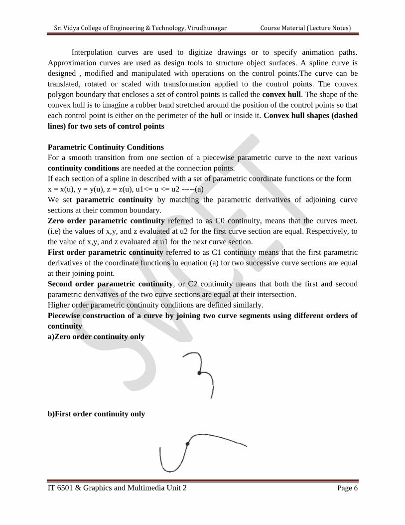
Parametric Continuity Conditions
For a smooth transition from one section of a piecewise parametric curve to the next various
continuity conditions are needed at the connection points.
If each section of a spline in described with a set of parametric coordinate functions or the form
x = x(u), y = y(u), z = z(u), u1<= u <= u2 -----(a)
We set parametric continuity by matching the parametric derivatives of adjoining curve
sections at their common boundary.
Zero order parametric continuity referred to as C0 continuity, means that the curves meet.
(i.e) the values of x,y, and z evaluated at u2 for the first curve section are equal. Respectively, to
the value of x,y, and z evaluated at u1 for the next curve section.
First order parametric continuity referred to as C1 continuity means that the first parametric
derivatives of the coordinate functions in equation (a) for two successive curve sections are equal
at their joining point.
Second order parametric continuity, or C2 continuity means that both the first and second
parametric derivatives of the two curve sections are equal at their intersection.
Higher order parametric continuity conditions are defined similarly.
Piecewise construction of a curve by joining two curve segments using different orders of
continuity
a)Zero order continuity only
b)First order continuity only
Sri Vidya College of Engineering & Technology, Virudhunagar Course Material (Lecture Notes)
IT 6501 & Graphics and Multimedia Unit 2 Page 7
c) Second order continuity only
Geometric Continuity Conditions
To specify conditions for geometric continuity is an alternate method for joining two successive
curve sections.
The parametric derivatives of the two sections should be proportional to each other at their
common boundary instead of equal to each other.
Zero order Geometric continuity referred as G0 continuity means that the two curves sections
must have the same coordinate position at the boundary point.
First order Geometric Continuity referred as G1 continuity means that the parametric first
derivatives are proportional at the interaction of two successive sections.
Second order Geometric continuity referred as G2 continuity means that both the first and second
parametric derivatives of the two curve sections are proportional at their boundary. Here the
curvatures of two sections will match at the joining position.
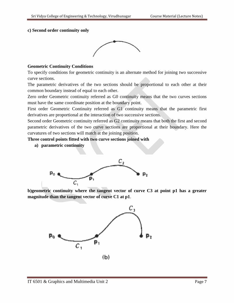
Three control points fitted with two curve sections joined with
a) parametric continuity
b)geometric continuity where the tangent vector of curve C3 at point p1 has a greater
magnitude than the tangent vector of curve C1 at p1.
Sri Vidya College of Engineering & Technology, Virudhunagar Course Material (Lecture Notes)
IT 6501 & Graphics and Multimedia Unit 2 Page 8
Spline specifications There are three methods to specify a spline representation:
1. We can state the set of boundary conditions that are imposed on the spline; (or)
2. We can state the matrix that characterizes the spline; (or)
3. We can state the set of blending functions that determine how specified geometric constraints
on the curve are combined to calculate positions along the curve path.
To illustrate these three equivalent specifications, suppose we have the following parametric
cubic polynomial representation for the x coordinate along the path of a spline section.
x(u)=axu3 + axu2 + cxu + dx 0<= u <=1 ----------(1) Boundary conditions for this curve might be
set on the endpoint coordinates x(0) and x(1) and on the parametric first derivatives at the
endpoints x’(0) and x’(1). These boundary conditions are sufficient to determine the values of
the four coordinates ax, bx, cx and dx. From the boundary conditions we can obtain the matrix
that characterizes this spline curve by first rewriting eq(1) as the matrix product
x(u) = [u3 u2 u1 1] ax
bx
cx -------( 2 )
dx
= U.C
where U is the row matrix of power of parameter u and C is the coefficient column matrix.
Using equation (2) we can write the boundary conditions in matrix form and solve for the
coefficient matrix C as
C = Mspline . Mgeom -----(3) Where Mgeom in a four element column matrix containing the
geometric constraint values on the spline and Mspline in the 4 * 4 matrix that transforms the
geometric constraint values to the polynomial coefficients and provides a characterization for the
spline curve.
Matrix Mgeom contains control point coordinate values and other geometric constraints.
We can substitute the matrix representation for C into equation (2) to obtain.
x (u) = U . Mspline . Mgeom ------(4)
The matrix Mspline, characterizing a spline representation, called the basis matriz is useful for
transforming from one spline representation to another.
Finally we can expand equation (4) to obtain a polynomial representation for coordinate x in
terms of the geometric constraint parameters.
x(u) = Σ gk. BFk(u) where gk are the constraint parameters, such as the control point
coordinates and slope of the curve at the control points and BFk(u) are the polynomial blending
functions.
Sri Vidya College of Engineering & Technology, Virudhunagar Course Material (Lecture Notes)
IT 6501 & Graphics and Multimedia Unit 2 Page 9
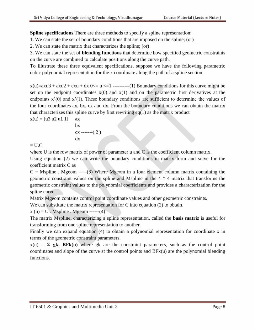
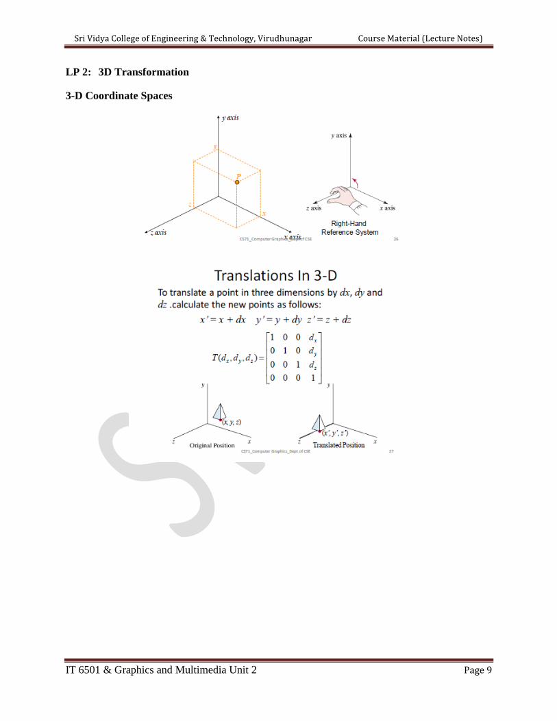
LP 2: 3D Transformation
3-D Coordinate Spaces
Sri Vidya College of Engineering & Technology, Virudhunagar Course Material (Lecture Notes)
IT 6501 & Graphics and Multimedia Unit 2 Page 10
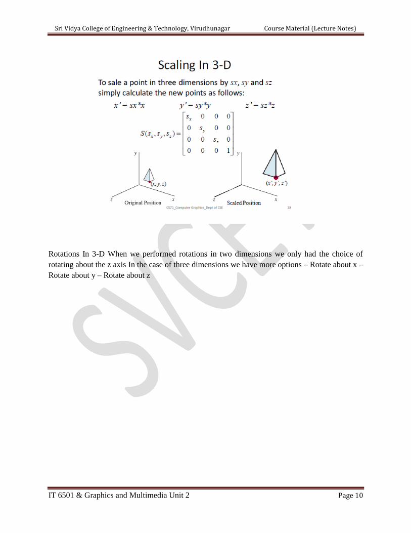
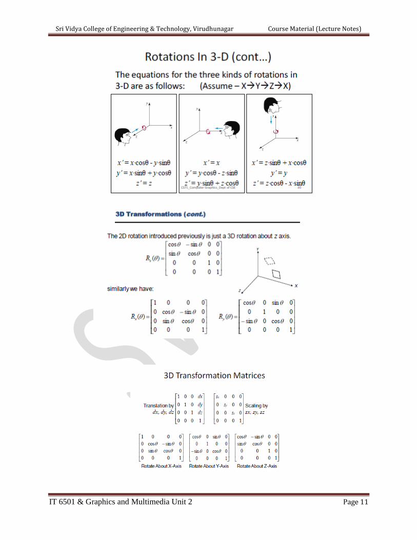
Rotations In 3-D When we performed rotations in two dimensions we only had the choice of
rotating about the z axis In the case of three dimensions we have more options – Rotate about x –
Rotate about y – Rotate about z
Sri Vidya College of Engineering & Technology, Virudhunagar Course Material (Lecture Notes)
IT 6501 & Graphics and Multimedia Unit 2 Page 11
Sri Vidya College of Engineering & Technology, Virudhunagar Course Material (Lecture Notes)
IT 6501 & Graphics and Multimedia Unit 2 Page 12
General 3D Rotations • Rotation about an axis that is parallel to one of the coordinate
axes : 1. Translate the object so that the rotation axis coincides with the parallel coordinate axis
2. Perform the specified rotation about the axis 3. Translate the object so that the rotation axis is
moved back to its original position • Not parallel : 1. Translate the object so that the rotation axis
passes through the coordinate origin 2. Rotate the object so that the axis of rotation coincides
with one of the coordinate axes 3. Perform the specified rotation about the axis 4. Apply inverse
rotations to bring the rotation axis back to its original orientation 5. Apply the inverse translation
to bring back the rotation axis to its original position
3 D Transformation functions • Functions are – translate3(translateVector, matrixTranslate) –
rotateX(thetaX, xMatrixRotate) – rotateY(thetaY, yMatrixRotate) – rotateZ(thetaZ,
zMatrixRotate) – scale3(scaleVector,matrixScale) • To apply transformation matrix to the
specified points , – transformPoint3(inPoint, matrix,outPoint) • We can construct composite
transformations with the following functions – composeMatrix3 – buildTransformationMatrix3 –
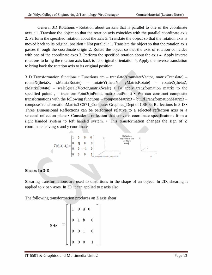
composeTransformationMatrix3 CS71_Computer Graphics_Dept of CSE 34 Reflections In 3-D •
Three Dimensional Reflections can be performed relative to a selected reflection axis or a
selected reflection plane • Consider a reflection that converts coordinate specifications from a
right handed system to left handed system. • This transformation changes the sign of Z
coordinate leaving x and y coordinates
Shears In 3-D
Shearing transformations are used to distortions in the shape of an object. In 2D, shearing is
applied to x or y axes. In 3D it can applied to z axis also
The following transformation produces an Z axis shear
1 0 a 0
0 1 b 0
SHz
0 0 1 0
0 0 0 1
Sri Vidya College of Engineering & Technology, Virudhunagar Course Material (Lecture Notes)
IT 6501 & Graphics and Multimedia Unit 2 Page 13
Parameters a and b can be assigned any real values
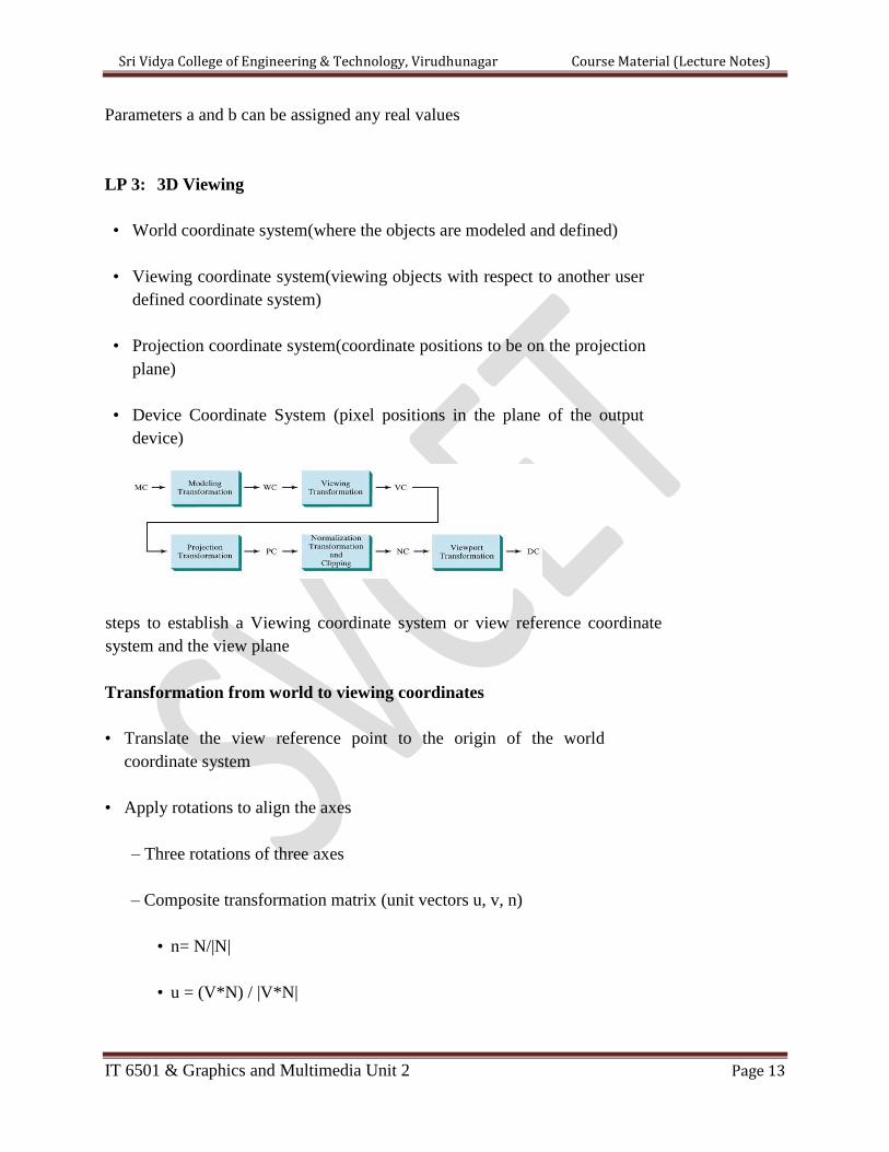
LP 3: 3D Viewing
• World coordinate system(where the objects are modeled and defined)
• Viewing coordinate system(viewing objects with respect to another user
defined coordinate system)
• Projection coordinate system(coordinate positions to be on the projection
plane)
• Device Coordinate System (pixel positions in the plane of the output
device)
steps to establish a Viewing coordinate system or view reference coordinate
system and the view plane
Transformation from world to viewing coordinates
• Translate the view reference point to the origin of the world
coordinate system
• Apply rotations to align the axes
– Three rotations of three axes
– Composite transformation matrix (unit vectors u, v, n)
• n= N/|N|
• u = (V*N) / |V*N|
Sri Vidya College of Engineering & Technology, Virudhunagar Course Material (Lecture Notes)
IT 6501 & Graphics and Multimedia Unit 2 Page 14
• v = n * u
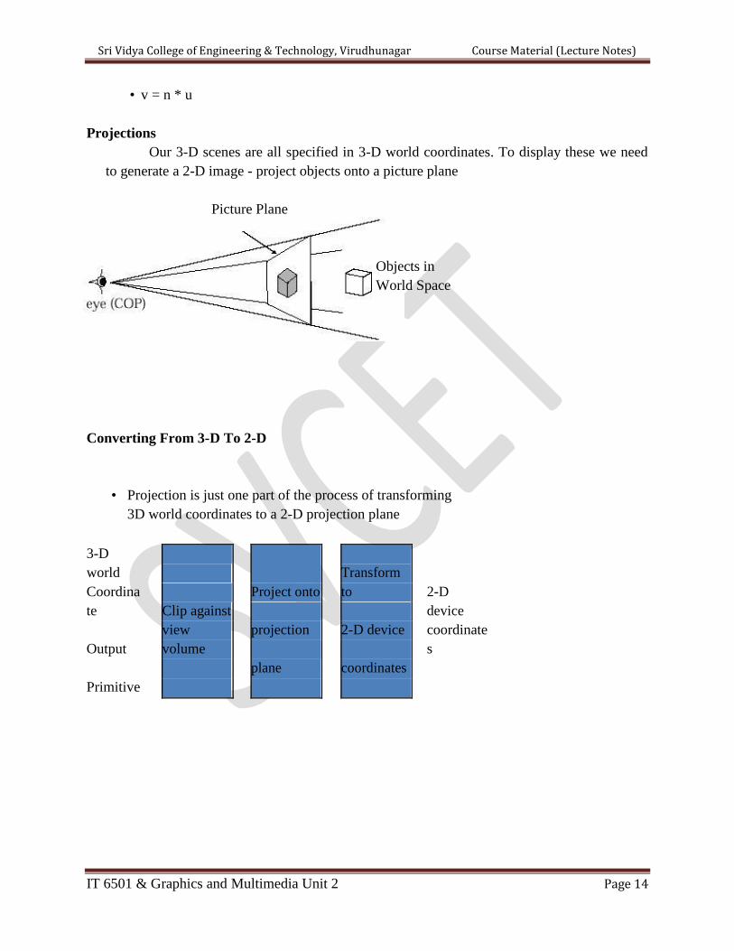
Projections
Our 3-D scenes are all specified in 3-D world coordinates. To display these we need
to generate a 2-D image - project objects onto a picture plane
Picture Plane
Objects in
World Space
Converting From 3-D To 2-D
• Projection is just one part of the process of transforming
3D world coordinates to a 2-D projection plane
3-D
world
Project onto
Transform
to
Coordina
te Clip against
2-D
device
projection
2-D device
Output
view
volume
coordinate
s
plane
coordinates
Primitive
Sri Vidya College of Engineering & Technology, Virudhunagar Course Material (Lecture Notes)
IT 6501 & Graphics and Multimedia Unit 2 Page 15
LP 5: Color Models
Color Model is a method for explaining the properties or behavior of color within some
particular context. No single color model can explain all aspects of color, so we make use of
different models to help describe the different perceived characteristics of color.
Properties of Light
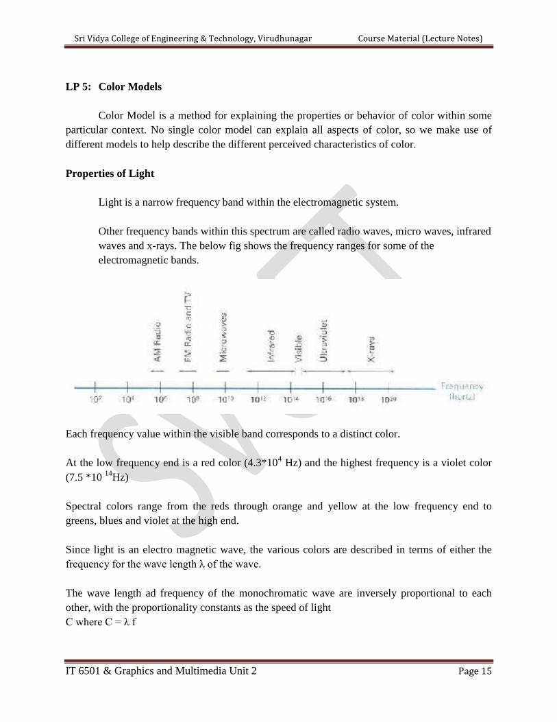
Light is a narrow frequency band within the electromagnetic system.
Other frequency bands within this spectrum are called radio waves, micro waves, infrared
waves and x-rays. The below fig shows the frequency ranges for some of the
electromagnetic bands.
Each frequency value within the visible band corresponds to a distinct color.
At the low frequency end is a red color (4.3*104 Hz) and the highest frequency is a violet color
(7.5 *10 14
Hz)
Spectral colors range from the reds through orange and yellow at the low frequency end to
greens, blues and violet at the high end.
Since light is an electro magnetic wave, the various colors are described in terms of either the
frequency for the wave length λ of the wave.
The wave length ad frequency of the monochromatic wave are inversely proportional to each
other, with the proportionality constants as the speed of light
C where C = λ f
Sri Vidya College of Engineering & Technology, Virudhunagar Course Material (Lecture Notes)
IT 6501 & Graphics and Multimedia Unit 2 Page 16
A light source such as the sun or a light bulb emits all frequencies within the visible range to
produce white light. When white light is incident upon an object, some frequencies are reflected
and some are absorbed by the object. The combination of frequencies present in the reflected
light determines what we perceive as the color of the object.
If low frequencies are predominant in the reflected light, the object is described as red. In this
case, the perceived light has the dominant frequency at the red end of the spectrum. The
dominant frequency is also called the hue, or simply the color of the light.
Brightness is another property, which in the perceived intensity of the light.
Intensity in the radiant energy emitted per limit time, per unit solid angle, and per unit projected
area of the source.
Radiant energy is related to the luminance of the source.
The next property in the purity or saturation of the light.
o Purity describes how washed out or how pure the color of the light appears.
o Pastels and Pale colors are described as less pure.
The term chromaticity is used to refer collectively to the two properties, purity and
dominant frequency.
Two different color light sources with suitably chosen intensities can be used to produce
a range of other colors.
If the 2 color sources combine to produce white light, they are called complementary
colors. E.g., Red and Cyan, green and magenta, and blue and yellow.
Color models that are used to describe combinations of light in terms of dominant
frequency use 3 colors to obtain a wide range of colors, called the color gamut.
The 2 or 3 colors used to produce other colors in a color model are called primary colors.
Standard Primaries
XYZ Color
The set of primaries is generally referred to as the XYZ or (X,Y,Z) color model
Sri Vidya College of Engineering & Technology, Virudhunagar Course Material (Lecture Notes)
IT 6501 & Graphics and Multimedia Unit 2 Page 17
where X,Y and Z represent vectors in a 3D, additive color space.
Any color Cλ is expressed as
Cλ = XX + YY + ZZ------------- (1)
Where X,Y and Z designates the amounts of the standard primaries needed
to match Cλ.
It is convenient to normalize the amount in equation (1) against luminance
(X+ Y+ Z). Normalized amounts are calculated as,
x = X/(X+Y+Z), y = Y/(X+Y+Z), z = Z/(X+Y+Z)
with x + y + z = 1
Any color can be represented with just the x and y amounts. The parameters x and y are
called the chromaticity values because they depend only on hue and purity.
If we specify colors only with x and y, we cannot obtain the amounts X, Y and Z. so, a
complete description of a color in given with the 3 values x, y and Y.
X = (x/y)Y, Z = (z/y)Y
Where z = 1-x-y.
Intuitive Color Concepts
Color paintings can be created by mixing color pigments with white and black
pigments to form the various shades, tints and tones.
Starting with the pigment for a „pure color‟ the color is added to black pigment to
produce different shades. The more black pigment produces darker shades.
Different tints of the color are obtained by adding a white pigment to the original color,
making it lighter as more white is added.
Tones of the color are produced by adding both black and white pigments.
Sri Vidya College of Engineering & Technology, Virudhunagar Course Material (Lecture Notes)
IT 6501 & Graphics and Multimedia Unit 2 Page 18
RGB Color Model
Based on the tristimulus theory of version, our eyes perceive color through the
stimulation of three visual pigments in the cones on the retina.
These visual pigments have a peak sensitivity at wavelengths of about 630 nm (red), 530
nm (green) and 450 nm (blue).
By comparing intensities in a light source, we perceive the color of the light.
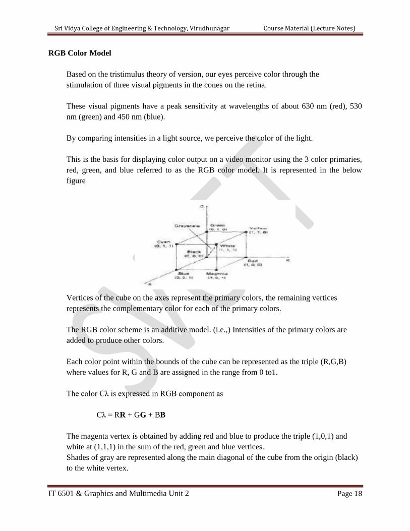
This is the basis for displaying color output on a video monitor using the 3 color primaries,
red, green, and blue referred to as the RGB color model. It is represented in the below
figure
Vertices of the cube on the axes represent the primary colors, the remaining vertices
represents the complementary color for each of the primary colors.
The RGB color scheme is an additive model. (i.e.,) Intensities of the primary colors are
added to produce other colors.
Each color point within the bounds of the cube can be represented as the triple (R,G,B)
where values for R, G and B are assigned in the range from 0 to1.
The color Cλ is expressed in RGB component as
Cλ = RR + GG + BB
The magenta vertex is obtained by adding red and blue to produce the triple (1,0,1) and
white at (1,1,1) in the sum of the red, green and blue vertices.
Shades of gray are represented along the main diagonal of the cube from the origin (black)
to the white vertex.
Sri Vidya College of Engineering & Technology, Virudhunagar Course Material (Lecture Notes)
IT 6501 & Graphics and Multimedia Unit 2 Page 19
YIQ Color Model
The National Television System Committee (NTSC) color model for forming the
composite video signal in the YIQ model.
In the YIQ color model, luminance (brightness) information in contained in the Y
parameter, chromaticity information (hue and purity) is contained into the I and Q
parameters.
A combination of red, green and blue intensities are chosen for the Y parameter to yield
the standard luminosity curve.
Since Y contains the luminance information, black and white TV monitors use only the Y
signal.
Parameter I contain orange-cyan hue information that provides the flash-tone shading and
occupies a bandwidth of 1.5 MHz.
Parameter Q carries green-magenta hue information in a bandwidth of about 0.6MHz.
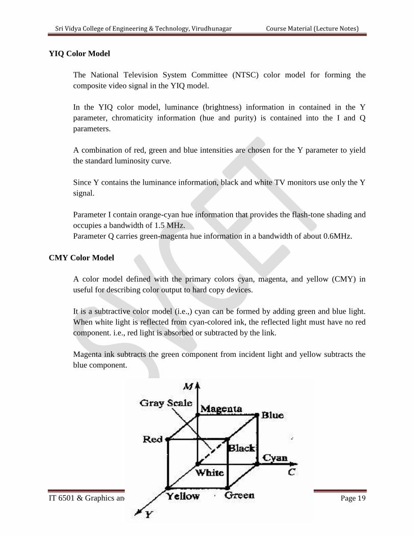
CMY Color Model
A color model defined with the primary colors cyan, magenta, and yellow (CMY) in
useful for describing color output to hard copy devices.
It is a subtractive color model (i.e.,) cyan can be formed by adding green and blue light.
When white light is reflected from cyan-colored ink, the reflected light must have no red
component. i.e., red light is absorbed or subtracted by the link.
Magenta ink subtracts the green component from incident light and yellow subtracts the
blue component.
Sri Vidya College of Engineering & Technology, Virudhunagar Course Material (Lecture Notes)
IT 6501 & Graphics and Multimedia Unit 2 Page 20
In CMY model, point (1,1,1) represents black because all components of the incident
light are subtracted.
The origin represents white light.
Equal amounts of each of the primary colors produce grays along the main diagonal of
the cube.
A combination of cyan and magenta ink produces blue light because the red and green
components of the incident light are absorbed.
The printing process often used with the CMY model generates a color point with a
collection of 4 ink dots; one dot is used for each of the primary colors (cyan, magenta and
yellow) and one dot in black.
The conversion from an RGB representation to a CMY representation is expressed as
[ ] [ ] [ ]
Where the white is represented in the RGB system as the unit column vector.
Similarly the conversion of CMY to RGB representation is expressed as
[ ] [ ] [ ]
Where black is represented in the CMY system as the unit column vector.
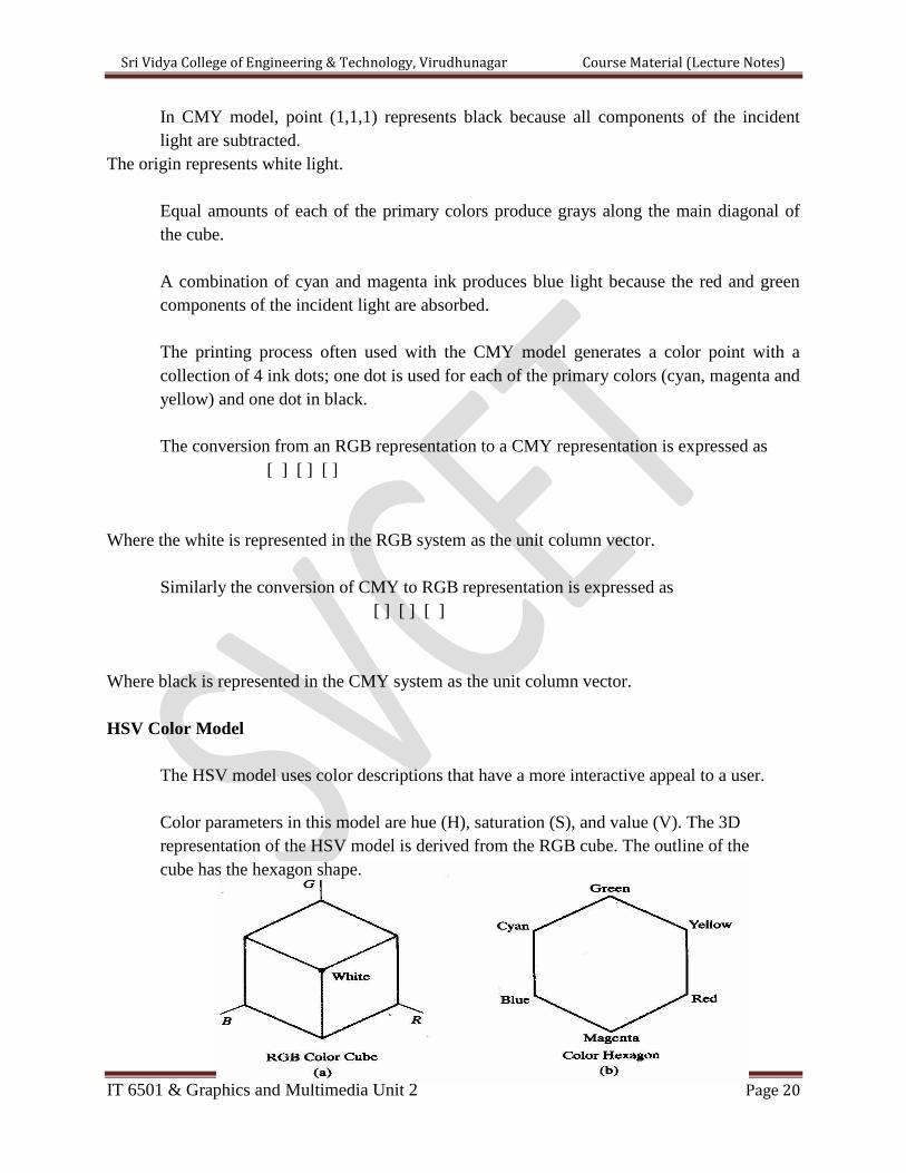
HSV Color Model
The HSV model uses color descriptions that have a more interactive appeal to a user.
Color parameters in this model are hue (H), saturation (S), and value (V). The 3D
representation of the HSV model is derived from the RGB cube. The outline of the
cube has the hexagon shape.
Sri Vidya College of Engineering & Technology, Virudhunagar Course Material (Lecture Notes)
IT 6501 & Graphics and Multimedia Unit 2 Page 21
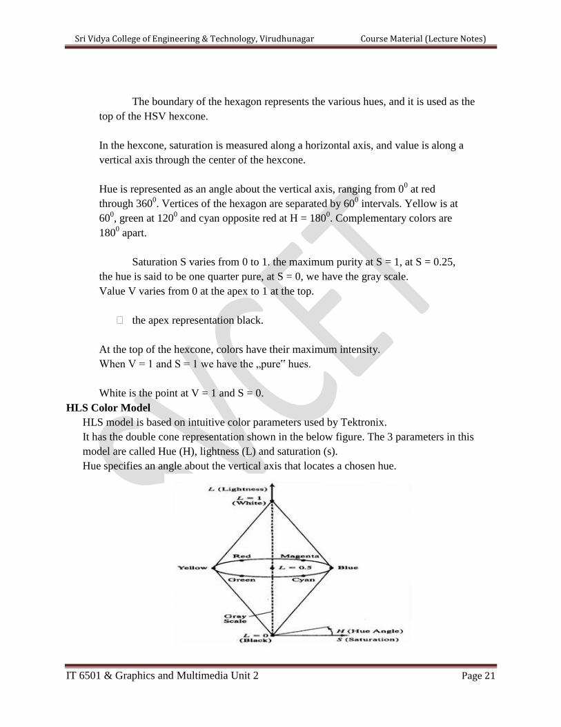
The boundary of the hexagon represents the various hues, and it is used as the
top of the HSV hexcone.
In the hexcone, saturation is measured along a horizontal axis, and value is along a
vertical axis through the center of the hexcone.
Hue is represented as an angle about the vertical axis, ranging from 00 at red
through 3600. Vertices of the hexagon are separated by 60
0 intervals. Yellow is at
600, green at 120
0 and cyan opposite red at H = 180
0. Complementary colors are
1800 apart.
Saturation S varies from 0 to 1. the maximum purity at S = 1, at S = 0.25,
the hue is said to be one quarter pure, at S = 0, we have the gray scale.
Value V varies from 0 at the apex to 1 at the top.
the apex representation black.
At the top of the hexcone, colors have their maximum intensity.
When V = 1 and S = 1 we have the „pure‟ hues.
White is the point at V = 1 and S = 0.
HLS Color Model
HLS model is based on intuitive color parameters used by Tektronix.
It has the double cone representation shown in the below figure. The 3 parameters in this
model are called Hue (H), lightness (L) and saturation (s).
Hue specifies an angle about the vertical axis that locates a chosen hue.
Sri Vidya College of Engineering & Technology, Virudhunagar Course Material (Lecture Notes)
IT 6501 & Graphics and Multimedia Unit 2 Page 22
In this model H = θ0 corresponds to Blue.
The remaining colors are specified around the perimeter of the cone in the same order as in
the HSV model.
Magenta is at 600, Red in at 120
0, and cyan in at H = 180
0.
The vertical axis is called lightness (L). At L = 0, we have black, and white is at L
= 1 Gray scale in along the L axis and the “purehues” on the L = 0.5 plane.
Saturation parameter S specifies relative purity of a color. S varies from 0 to 1 pure hues
are those for which S = 1 and L = 0.
As S decreases, the hues are said to be less pure.
At S= 0, it is said to be gray scale.
LP 7: Animation
Computer animation refers to any time sequence of visual changes in a scene.
Computer animations can also be generated by changing camera parameters such as
position, orientation and focal length.
Applications of computer-generated animation are entertainment, advertising,
training and education.
Example : Advertising animations often transition one object shape into another.
Frame-by-Frame animation
Each frame of the scene is separately generated and stored. Later, the frames can be recoded
on film or they can be consecutively displayed in "real-time playback" mode
Design of Animation Sequences
An animation sequence in designed with the following steps:
o Story board layout
o Object definitions
o Key-frame specifications
Sri Vidya College of Engineering & Technology, Virudhunagar Course Material (Lecture Notes)
IT 6501 & Graphics and Multimedia Unit 2 Page 23
Story Board:
Generation of in-between frames.
The story board is an outline of the action.
It defines the motion sequences as a set of basic events that are to take place.
Depending on the type of animation to be produced, the story board could consist
of a set of rough sketches or a list of the basic ideas for the motion.
Object Definition
An object definition is given for each participant in the action.
Objects can be defined in terms of basic shapes such as polygons or splines.
The associated movements of each object are specified along with the shape.
Key frame
A key frame is detailed drawing of the scene at a certain time in the animation
sequence.
Within each key frame, each object is positioned according to the time for that frame.
Some key frames are chosen at extreme positions in the action; others are spaced so that
the time interval between key frames is not too much.
In-betweens
In betweens are the intermediate frames between the key frames.
The number of in between needed is determined by the media to be used to display
the animation.
Film requires 24 frames per second and graphics terminals are refreshed at the rate of
30 to 60 frames per seconds.
Time intervals for the motion are setup so there are from 3 to 5 in-between for each

Sri Vidya College of Engineering & Technology, Virudhunagar Course Material (Lecture Notes)
IT 6501 & Graphics and Multimedia Unit 2 Page 24
pair of key frames.
Depending on the speed of the motion, some key frames can be duplicated.
For a 1 min film sequence with no duplication, 1440 frames are needed.
Other required tasks are
Motion verification
Editing
Production and synchronization of a sound track.
General Computer Animation Functions
Steps in the development of an animation sequence are,
Object manipulation and rendering
Camera motion
Generation of in-betweens
Animation packages such as wave front provide special functions for designing the
animation and processing individuals objects.
Animation packages facilitate to store and manage the object database.
Object shapes and associated parameter are stored and updated in the database.
Motion can be generated according to specified constraints using 2D and 3D
transformations.
Standard functions can be applied to identify visible surfaces and apply the
rendering algorithms.
Camera movement functions such as zooming, panning and tilting are used for
motion simulation.
Sri Vidya College of Engineering & Technology, Virudhunagar Course Material (Lecture Notes)
IT 6501 & Graphics and Multimedia Unit 2 Page 25
Given the specification for the key frames, the in-betweens can be automatically
generated.
Raster Animations
On raster systems, real-time animation in limited applications can be generated using
raster operations.
Sequence of raster operations can be executed to produce real time animation of either
2D or 3D objects.
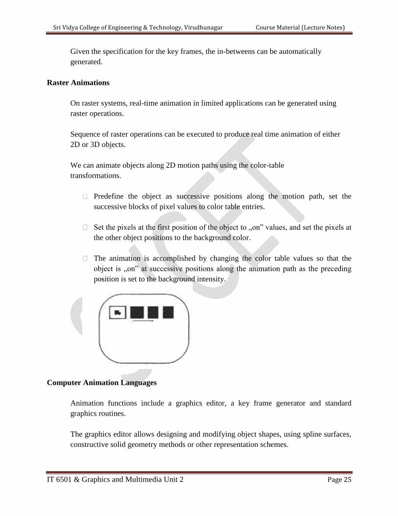
We can animate objects along 2D motion paths using the color-table
transformations.
Predefine the object as successive positions along the motion path, set the
successive blocks of pixel values to color table entries.
Set the pixels at the first position of the object to „on‟ values, and set the pixels at
the other object positions to the background color.
The animation is accomplished by changing the color table values so that the
object is „on‟ at successive positions along the animation path as the preceding
position is set to the background intensity.
Computer Animation Languages
Animation functions include a graphics editor, a key frame generator and standard
graphics routines.
The graphics editor allows designing and modifying object shapes, using spline surfaces,
constructive solid geometry methods or other representation schemes.
Sri Vidya College of Engineering & Technology, Virudhunagar Course Material (Lecture Notes)
IT 6501 & Graphics and Multimedia Unit 2 Page 26
Scene description includes the positioning of objects and light sources defining the
photometric parameters and setting the camera parameters.
Action specification involves the layout of motion paths for the objects and camera.
Keyframe systems are specialized animation languages designed dimply to generate the
in-betweens from the user specified keyframes.
Parameterized systems allow object motion characteristics to be specified as part of the
object definitions. The adjustable parameters control such object characteristics as
degrees of freedom motion limitations and allowable shape changes.
Scripting systems allow object specifications and animation sequences to be defined with
a user input script. From the script, a library of various objects and motions can be
constructed.
Keyframe Systems
Each set of in-betweens are generated from the specification of two keyframes.
For complex scenes, we can separate the frames into individual components or objects
called cells, an acronym from cartoon animation.
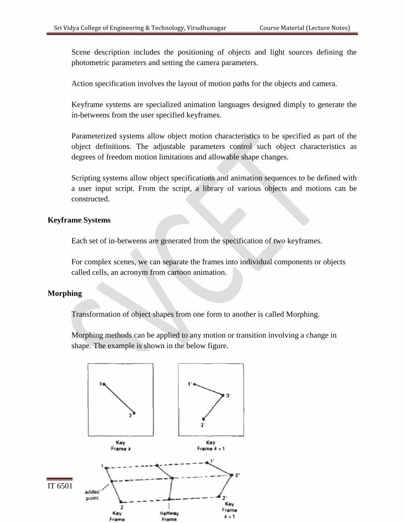
Morphing
Transformation of object shapes from one form to another is called Morphing.
Morphing methods can be applied to any motion or transition involving a change in
shape. The example is shown in the below figure.
Sri Vidya College of Engineering & Technology, Virudhunagar Course Material (Lecture Notes)
IT 6501 & Graphics and Multimedia Unit 2 Page 27
Suppose we equalize the edge count and parameters Lk and Lk+1 denote the
number of line segments in two consecutive frames. We define,
Lmax = max (Lk, Lk+1)
Lmin = min(Lk , Lk+1)
Ne = Lmax mod Lmin
Ns = int (Lmax/Lmin)
The preprocessing is accomplished by
Dividing Ne edges of keyframemin into Ns+1 section.
Dividing the remaining lines of keyframemin into Ns sections.
For example, if Lk = 15 and Lk+1 = 11, we divide 4 lines of keyframek+1 into 2
sections each. The remaining lines of keyframek+1 are left infact.
If the vector counts in equalized parameters Vk and Vk+1 are used to denote the
number of vertices in the two consecutive frames. In this case we define
Vmax = max(Vk,Vk+1), Vmin = min( Vk,Vk+1) and
Nls = (Vmax -1) mod (Vmin – 1)
Np = int ((Vmax – 1)/(Vmin – 1 ))
Preprocessing using vertex count is performed by
Adding Np points to Nls line section of keyframemin.
Adding Np-1 points to the remaining edges of keyframemin.
Simulating Accelerations
Curve-fitting techniques are often used to specify the animation paths between key frames.
Given the vertex positions at the key frames, we can fit the positions with linear or nonlinear
paths. Figure illustrates a nonlinear fit of key-frame positions. This determines the trajectories
for the in-betweens. To simulate accelerations, we can adjust the time spacing for the in-
betweens.
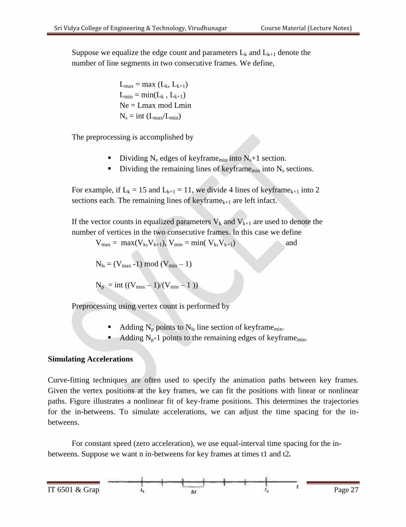
For constant speed (zero acceleration), we use equal-interval time spacing for the in-
betweens. Suppose we want n in-betweens for key frames at times t1 and t2.
Sri Vidya College of Engineering & Technology, Virudhunagar Course Material (Lecture Notes)
IT 6501 & Graphics and Multimedia Unit 2 Page 28
The time interval between key frames is then divided into n + 1 subintervals, yielding an in-
between spacing of
∆= t2-t1/n+1
we can calculate the time for any in-between as
tBj = t1+j ∆t, j = 1,2, . . . . . . n
Motion Specification
These are several ways in which the motions of objects can be specified in an
animation system.
Direct Motion Specification
Here the rotation angles and translation vectors are explicitly given.
Then the geometric transformation matrices are applied to transform coordinate
positions.
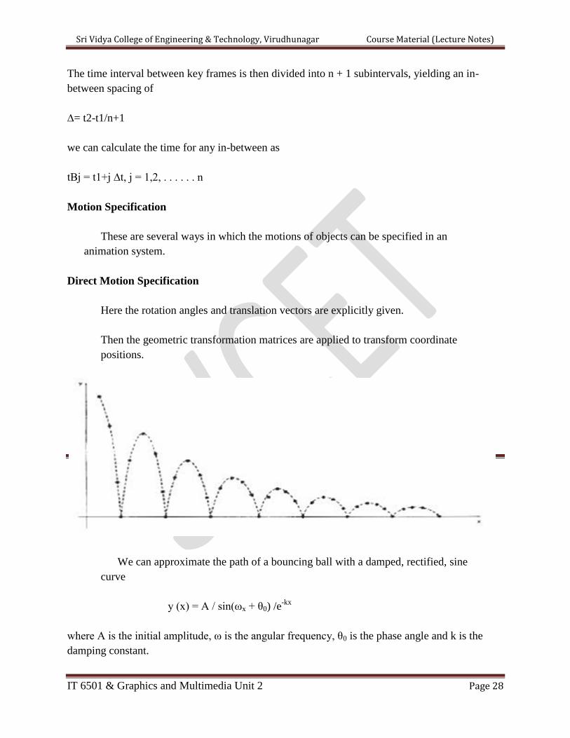
We can approximate the path of a bouncing ball with a damped, rectified, sine
curve
y (x) = A / sin(ωx + θ0) /e-kx
where A is the initial amplitude, ω is the angular frequency, θ0 is the phase angle and k is the
damping constant.
Recommended