LA-13307-M5
Summay of the Models and
Methods for the FE_E7M
Application –A Finite-Element
Heat- and Mass-T’’ansfer Code
Los AlamosNATIONAL LABORATORY
Los Alarnos National Laboratory is operated by the University of Cal~orniajbr the United Sfafes Deparfmenf of Energy under confracf W-7405-ENG-36
This work was supported by the Yucca Mountain Site CharacterizationProject Oji2e as part of the Civilian Radioactive Waste ManagementProgram of the U.S. Department of Energy.
An A-ffirmative Acfion/Equal Opportunity Employer
This report wns prepnred m m nccount of work sponsored by m ngencyof the United StafesGovernment. Mfher the Regents of the University of Ciiljbrnin, the United Stafes Governmentnor my agency fhereqf, nor my of fha”r employees, nwkes my wmmnfy, express or implied, orossznnes my legsil liability or responszbilify for fhe occunwy, completeness, or usefulness of myinfornmtion, sippvnwfus, producf, or process disclosed, or represents fhaf ifs use would nof infringepriuntely owned rights. Rq&rence herein fo my spec$c commercial producf, process, or service bytrade rmme, frademark, nzan@cfurer, or otheiwise, does nof necessm-ily consfif ufe or imply ifsendorsement, recommendsition, or favoring by the Regents of fife University of Cal$orniu, theUnifed Sfates Government, or any agency thereof The views and opinions of authors expressedherein do not necemrily state or reflecf those of fhe Regents of fhe University of California, fheUnifed States Govemnenf, or any ngency thereof. The Los Ahnnos Mfionaf Labcmfory sfronglysupports academic freedom and n researcher’sright to publish; as an ins fifnfion, however, fheLiiborafory does nof endorse the viewpoint of a publication or guarantee its technical correctness.

DISCLAIMER
Portions of this document may be illegiblein electronic image products. images areproduced from the best available originaldocument.
Summary of tlze Models and
Methods for the FEHM
Application –A Finite-Element
Heat- and Mass-Transfer Code
George A. Zyvoloslci
Bruce A. Robinson
Zora V Dash
Lynn L. Trease
LA-13307-MS
UC-800 and UC-802Issued: July 1997


TABLE OF CONTENTS
CONTENTS
Summarv of Models and Methods for the FEHM Application
TABLE OF
TABLE OF CONTENTS . . . . . . . . . . . . . . . . . . . . . . . . . . . . . . . . . . . . . . . . . . . . . . . . . . . . . . . . . . . . ..V
LIST OF FIGURES . . . . . . . . . . . . . . . . . . . . . . . . . . . . . . . . . . . . . . . . . . . . . . . . . . . . . . . . . . . . . . . ..Vii
LIST OF TABLES . . . . . . . . . . . . . . . . . . . . . . . . . . . . . . . . . . . . . . . . . . . . . . . . . . . . . . . . . . . . . . . . ..viii
ABSTRACT . . . . . . . . . . . . . . . . . . . . . . . . . . . . . . . . . . . . . . . . . . . . . . . . . . . . . . . . . . . . . . . . . . . . . . ...1
1.0.
2.0.
3.0.
4.0.
5.0.
6.0.
7.0.
8.0.
PURPOSE . . . . . . . . . . . . . . . . . . . . . . . . . . . . . . . . . . . . . . . . . . . . . . . . . . . . . . . . . . . . . . . . . ...2
DEFINITIONSANDACRONYMS. . . . . . . . . . . . . . . . . . . . . . . . . . . . . . . . . . . . . . . . . . . . . . ...2
2.1. Definitions . . . . . . . . . . . . . . . . . . . . . . . . . . . . . . . . . . . . . . . . . . . . . . . . . . . . . . . . . . . . . ...2
2.2. Acronyms . . . . . . . . . . . . . . . . . . . . . . . . . . . . . . . . . . . . . . . . . . . . . . . . . . . . . . . . . . . . . . . ..2
REFERENCES . . . . . . . . . . . . . . . . . . . . . . . . . . . . . . . . . . . . . . . . . . . . . . . . . . . . . . . . . . . . . ...2
NOTATION . . . . . . . . . . . . . . . . . . . . . . . . . . . . . . . . . . . . . . . . . . . . . . . . . . . . . . . . . . . . . . . . ...5
STATEMENTAND DESCRIPTION OF THE PROBLEM . . . . . . . . . . . . . . . . . . . . . . . . . . ...12
STRUCTUREOFTHESYSTEMMODEL . . . . . . . . . . . . . . . . . . . . . . . . . . . . . . . . . . . . . . ...13
GENERAL NUMERICALPROCEDURE . . . . . . . . . . . . . . . . . . . . . . . . . . . . . . . . . . . . . . . ...13
COMPONENTMODELS . . . . . . . . . . . . . . . . . . . . . . . . . . . . . . . . . . . . . . . . . . . . . . . . . . . . ...15
8.1. Flow and Energy-Transport Equations . . . . . . . . . . . . . . . . . . . . . . . . . . . . . . . . . . . . . ...15
Purpose
Assumptions and limitations
Derivation
Applications
Numerkalmethod type
Derivation ofnumerical model
Location
Numerical stability and accuracy
Alternatives
8.2. Dual-PorosityandDouble-Porosity/Double-Permeability Formulation . . . . . . . . . . . . . . .28
Purpose
Assumptions and limitations
Derivation
Application
Numericalmethod type
Derivation ofnumerical model
Location
Numerical stability and accuracy
Alternatives
v
Summarv of Models and Methods for the FEHM ApplicationTABLE OF CONTENTS
8.3.
8.4.
Solute Transport Models: Reactive Transport and Particle Tracking. . . . . . . . . . . . . ...35
Purpose
Assumptions and limitations
Derivation
Applications
Numerical method type
Derivation of numerical model
Location
Numerical stability and accuracy
Alternatives
Constitutive Relationships . . . . . . . . . . . . . . . . . . . . . . . . . . . . . . . . . . . . . . . . . . . . . . . 53
Purpose
Assumptions and limitations
Derivation
Application
Numerical method type
Derivation of numerical model
Location
Numerical stability and accuracy
Alternatives
9.0. EXPERIENCE . . . . . . . . . . . . . . . . . . . . . . . . . . . . . . . . . . . . . . . . . . . . . . . . . . . . . . . . . ...-...61
10.O. APPENDIX . . . . . . . . . . . . . . . . . . . . . . . . . . . . . . . . . . . . . . . . . . . . . . . . . . . . . . . . . . . . . . . ...62
vi
Figure 1.
Figure 2.
Figure 3.
Figure 4.
Figure 5.
Summary of Models and Methods for the FEHM ApplicationLIST OF FIGURES
LIST OF FIGURES
Simplified diagram of code flow in the FEHM application. . . . . . . . . . . . . . . . . . . . . . ..14
Comparison of nodal connections for conventional and Lobatto integrations
foran orthogonal grid . . . . . . . . . . . . . . . . . . . . . . . . . . . . . . . . . . . . . . . . . . . . . . . . . . ...22
Area projections and internode distances used in finite-volume calculations on
aDelaunay grid . . . . . . . . . . . . . . . . . . . . . . . . . . . . . . .. . . . . . . . . . . . . . . . . . . . . . . . . ...23
Computational volume elements showing dual-porosity and double-porosity/
double-permeability parameters. . . . . . . . . . . . . . . . . . . . . . . . . . . . . . . . . . . . . . . . . . ...30
Model system used to formulate the residence-time transfer function for
matrix diffusion . . . . . . . . . . . . . . . . . . . . . . . . . . . . . . . . . . . . . . . . . . . . . . . . . . . . . . . . ..45
vii
Table I. Nomenclature . . . . . . . . . . . . . . . . . . . . . . . . . . . . . . . . . . . . . . . . . . . . . . . . . . . . . . . . . ...5
Table II. Sorption isotherm models . . . . . . . . . . . . . . . . . . . . . . . . . . . . . . . . . . . . . . . . . . . . . . . ...37
Table III. Polynomial coeffkients forenthalpy, density andviscosityfunctions . . . . . . . . . . . . ...62
Table IV. Polynomial coeffkients for saturationfunctions . . . . . . . . . . . . . . . . . . . . . . . . . . . . . ...63
Vlll
SummaryofModels andMethodsforthe FEHMApplicationLISTOFTABLES
LIST OF TABLES

Summary of Models and Methods for the FEHM Application—A Finite-Element Heat- and Mass-Transfer Code
by
George A. Zyvoloski, Bruce A. Robinson, Zora V. Dash, and Lynn L. Trease
ABSTRACT
The mathematical models and numerical methods employed by the FEHM application, a finite-
element heat- and mass-transfer computer code that can simulate nonisothermal multiphase multi-
component flow in porous media, are described. The use of this code is applicable to natural-state
studies of geothermal systems and groundwater flow. A primary use of the FEHM application will be
to assist in the understanding of flow fields and mass transport in the saturated and unsaturated zones
below the proposed Yucca Mountain nuclear waste repository in Nevada. The component models of
FEHM are discussed. The first major component, Flow- and Energy-Transport Equations, deals with
heat conduction; heat and mass transfer with pressure- and temperature-dependent properties, rela-
tive permeabilities and capillary pressures; isothermal air-water transport; and heat and mass trans-
fer with noncondensible gas. The second component, Dual-Porosity and Double-Porosity/Double-
Permeability Formulation, is designed for problems dominated by fracture flow. Another component,
The Solute-Transport Models, includes both a reactive-transport model that simulates transport of
multiple solutes with chemical reaction and a particle-tracking model. Finally, the component, Consti-
tutive Relationships, deals with pressure- and temperature-dependent fluid/air/gas properties, relative
permeabilities and capillary pressures, stress dependencies, and reactive and sorbing solutes. Each of
these components is discussed in detail, including purpose, assumptions and limitations, derivation,
applications, numerical method type, derivation of numerical model, location in the FEHM code flow,
numerical stability and accuracy, and alternative approaches to modeling the component.
1

Summary of Models and Methods for the FEHM ApplicationPURPOSE
1.0
2.0
3.0
PURPOSE
This models-and-methods summary provides a detailed description of the mathematical
models and numerical methods employed by the FEHM application.
DEFINITIONS AND ACRONYMS
2.1
2.2
DefinitionsFEHM: Finite-element heat- and mass-transfer code (Zyvoloski et al. 1988).
FEH~ an earlier verion of FEHM designed specifically for the Yucca Mountain
Site Characterization Project. Both versions are now equivalent, and the use of
FEHMN has been dropped.
AcronymsLANL: Los Alamos National Laboratory.
RTD: residence-time distribution.
RTTF: residence-time transfer function.
SOR: simultaneous over-relaxation.
YMP: Yucca Mountain Site Characterization Project.
REFERENCES
Birdsell, K. H., K. Campbell, K. G. Eggert, and B. J. Travis. 1990. Simulation of
radionuclide retardation at Yucca Mountain using a stochastic mineralogical/
geochemical model. In High Level Radioactive Waste Management: Proceedings of the
First International Topical Meeting, Las Vegas, Nevada, April 8–12, 1990, pp. 1.53-162.
La Grange Park, Illinois: American Nuclear Society.
Brigham, W. E. 1974. Mixing equations in short laboratory cores. Society of Petroleum
Engineers Journal 14: 91–99.
Brownell, D. H., S. K. Garg, and J. W. Pritchett. 1975. Computer simulation of
geothermal reservoirs. Paper SPE 5381 in Proceedings of the 45th California Regional
Meeting of the Society of Petroleum Engineers of AIME, Ventura, California. Richardson
Texas: Society of Petroleum Engineers.
Bullivant, D., and G. A. Zyvoloski. 1990. An efficient scheme for the solution of linear
system arising from coupled differential equations. Los Alamos National Laboratory
report LA-UR-90-3 187.
Corey, A. T. 1954. The interrelation between gas and oil relative permeabilities.
Producers Monthly 19:38-41.
Dalen, V. 1979. Simplified finite-element models for reservoir flow problems. Society of
Petroleum Engineers Journal 19; 333–343.
.
2

Summary of Models and Methods for the FEHM ApplicationREFERENCES
Dash, Z. V., B. A. Robinson, and G. A. Zyvoloski. 1997. Software design, requirements,
and validation for the FEHM application—a finite-element mass- and heat-transfer
code. Los Alamos National Laboratory report LA-13305-MS (May),
Friedly, J. C., and J. Rubin. 1992. Solute transport with multipIe equilibrium-
controlled or kinetically controlled chemical reactions. Water Resources Research 28(6):
1935–1953.
Fung, L. S. K., L. Buchanan, and R. Sharma. 1994. Hybrid-CVFE method for flexible-
grid reservoir simulation. Society of Petroleum Engineers Journal 19: 188–199.
Gangi, A. F. 1978. Variation of whole and fractured porous rock permeability with
confining pressure. International Journal of Rock Mechanics and Mining Sciences and
Geomechanics Abstracts 15: 249–157.
Harr, L., J. Gallagher, and G. S. Ken. 1984. NBS/NRC Steam Tables,
Thermodynamics, and Transport Properties and Computer Programs for Vapor and
Liquid States of Water. Washington: Hemisphere Publishing Corporation.
Hinton, E., and D. R. J. Owen. 1979. An Introduction to Finite Element Computations.
Swansea, Wales: Pineridge Press.
Klavetter, E. A., and R. R. Peters. 1986. Estimation of hydrologic properties of an
unsaturated fractured rock mass. Sandia National Laboratories report SAND84-2642.
Lu, N. 1994. A semianalytical method of path line computation for transient finite-
difference groundwater flow models. Water Resources Research 30(8): 2449–2459.
Maloszewski, P., and A. Zuber. 1985. On the theory of tracer experiments in fissured
rocks with a porous matrix. Journal of Hydrology 79: 333–358.
Mercer, J. W., and C. R. Faust. 1975. Simulation of water- and vapor-dominated
hydrothermal reservoirs. Paper SPE 5520 in Proceedings of the 50th Annual Fall
Meeting of the Society of Petroleum Engineers of AIME, Dallas, Texas. Richardson
Texas: Society of Petroleum Engineers.
Moench, A. F. 1984. Double-porosity models for a fissured groundwater reservoir with
fracture skin. Water Resources Reseach 20(7): 831–846.
Neretnicks, I. 1980. Diffusion in the rock matrix: An important factor in radionuclide
migration? Journal of Geophysical Research 85(B8): 43794397.
Nitao, J. 1988. Numerical modeling of the thermal and hydrological environment
around a nuclear waste package using the equivalent continuum approximation:
Horizontal emplacement. Lawrence Livermore National Laboratory report UCID-21444.
Plummer, L. N., and E. Busenberg. 1982. The solubilities of caIcite, argonite, and
vaterite in C02-H20 solutions between O and 90°C, and an evaluation of the aqueous
model for the system CaC03-H20. Geochimica et Cosmochimica Acts 46: 1101.
Polzer, W. L., M. G. Rae, H. R. Fuentes, and R. J. Beckman. 1992. Thermodynamically
derived relationships between the modified Langmuir isotherm and experimental
parameters. Environmental Science and Technology 26: 1780–1786.
Pruess, K. 1991. TOUGH2 - a general-purpose numerical simulator for multiphase
fluid and heat flow. Lawrence Berkeley Laboratory report LBL-29400.
3

Summary of Models and Methods for the FEHM ApplicationREFERENCES
Reeves, M., N. A. Baker, and J. O. Duguid. 1994. Review and selection of unsaturated
flow models. Civilian Radioactive Waste Management and Operation Contractor report
BOOOOOOOO-01425-2200 -OOO01 (Intera).
Reimus, P. W. 1995. The use of synthetic colloids in tracer transport experiments in
saturated rock fractures. Ph.D. thesis, the University of New Mexico, Albuquerque,
New Mexico.
Robinson, B. A. 1993. Model and methods summary for the SORBEQ application. Los
Alamos National Laboratory document SORBEQ MMS, ECD-20.
Robinson, B. A. 1994. A strategy for validating a conceptual model for radionuclide
migration in the saturated zone beneath Yucca Mountain. Radioactive Waste
Management and Environmental Restoration 19: 73–96.
Starr, R. C., R. W. Gillham, and E. A. Sudicky. 1985. Experimental investigation of
solute transport in stratified porous media 2: The reactive case. Water Resources
Research 21(7): 1043–1050.
Sychev, V. V., T. B. Selover, and G. E. Slark. 1988. Thermodynamic Properties of Air.
Washington: Hemisphere Publishing Corporation.
Tang, D. H., E. O. Frind, and E. A. Sudicky. 1981. Contaminant transport in fractured
porous media: Analytical solution for a single fracture. Water Resources Research 17(3):
555–564.
Tompson, A. F. B., and L. W. Gelhar. 1990. Numerical simulation of solute transport in
three-dimensional, randomly heterogeneous porous media. Water Resources Research
26(10): 2541–2562.
van Genuchten, M. T. 1980. A closed form equation for predicting hydraulic
conductivity of unsaturated soils. S~il Science Society of America Journal 44: 892–898.
Warren, J. E., and P. J. Root. 1963. The behavior of naturally fractured reservoirs.
Society of Petroleum Engineers Journal 3: 245–255.
Weeks, E. P. 1987. Effect of topography on gas flow in unsaturated fractured rock:
Concepts and observations. Proceedings of the American Geophysical Union Symposium
on Flow and Transport in Unsaturated Fractured Rock, D. Evans and T. Nicholson,
editors. Geophysical Monograph 42. Washington, D. C.: American Geophysical Union.
Yeh, G. T., and V. S. Tripathi. 1989. A critical evaluation of recent developments in
hydrogeochemical transport models of reactive multichemical components. Water
Resources Research 25: 93–108.
Young, L. C. 1981. A finite-element method for reservoir simulation. Society of
Petroleum Engineers Journal 21: 115–128.
Zienkiewicz, O. C. 1977. The Finite Element Method. London: McGraw-Hill.
Zienkiewicz, O. C., and C. J. Parekh. 1973. Transient field problems—two- and three-
dimensional analysis by isoparametric finite elements. International Journal of
Numerical Methods in Engineering 2: 61–70.
Zyvoloski, G. 1983. Finite-element methods for geothermal reservoir simulation.
International Journal for Numerical and Analytical Methods in Geomechanics 7: 75–86.
4
4.0
Summary of Models and Methods for the FEHM ApplicationNOTATION
Zyvoloski, G. A., and Z. V. Dash. 1991. Software verification report: FEHMN version
1.0. Los Alamos National Laboratory report LA-UR-91-609.
Zyvoloski, G. A., M. J. O’Sullivan, and D. E. Kro. 1979. Finite-difference techniques for
modeling geothermal reservoirs. International Journal for Numerical and Analytical
Methods in Geomechanic.s 3: 355–366.
Zyvoloski, G. A., Z. V. Dash, and S. Kelkar. 1988. FEHM: Finite-element heat- and
mass-transfer code. Los Alamos National Laboratory report LA-11224-MS.
Zyvoloski, G. A., Z. V. Dash, and S. Kelkar. 1992. FEHMN 1.0: Finite-element heat-
and mass-transfer code. Los Alamos National Laboratory report LA-12062-MS, Rev. 1.
Zyvoloski, G. A., and B. A. Robinson. 1995. Models and methods summary for the
GZSOLVE application. Los Alamos National Laboratory software document ECD-97.
Zyvoloski, G. A., B. A. Robinson, Z. V. Dash, and L. L. Trease. 1997. User’s manual for
the FEHM application—a finite-element mass- and heat-transfer code. Los Alamos
National Laboratory report LA-13306-M (May).
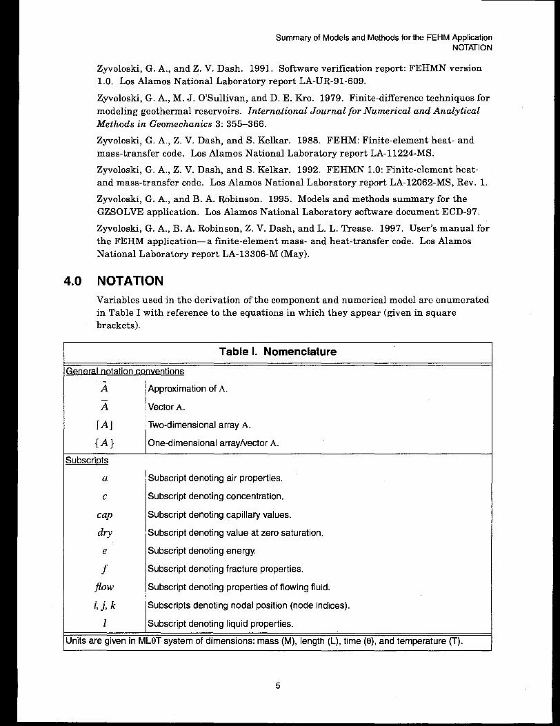
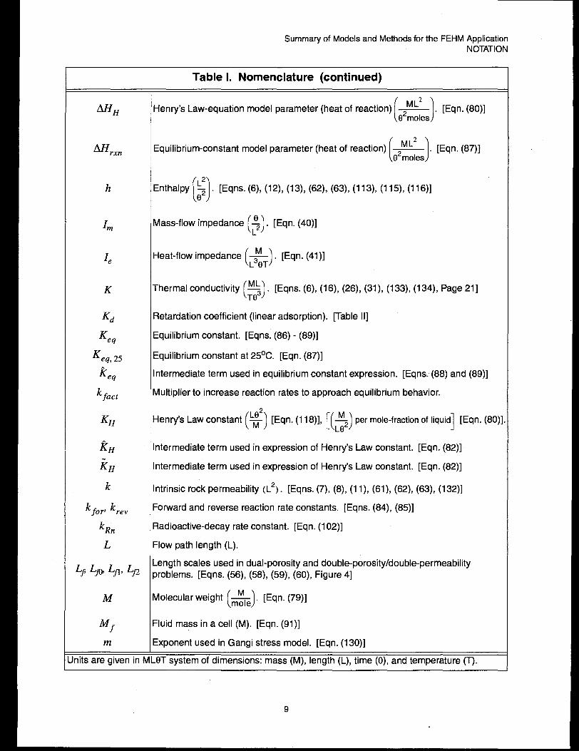
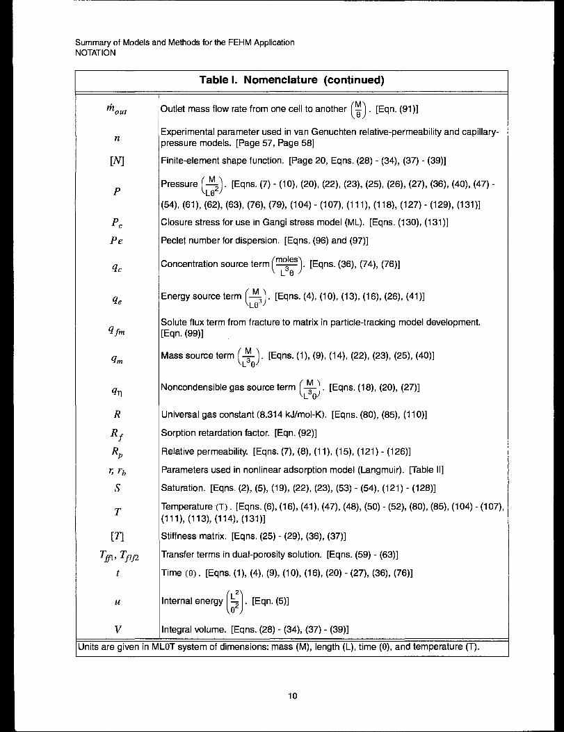
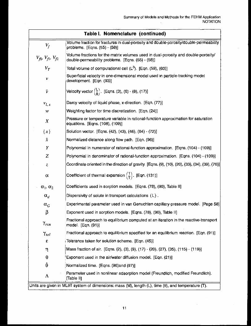
NOTATION
Variables used in the derivation of the component and numerical model are enumerated
in Table I with reference to the equations in which they appear (given in square
brackets).
Table 1. Nomenclature
;eneral notation conventions
i Approximation of A.
z Vector A.
[A] Two-dimensional array A.
{A} One-dimensional array/vector A.
hIbSCriDk
a Subscript denoting air properties.
c Subscript denoting concentration.
cap Subscript denoting capillary values.
dry Subscript denoting value at zero saturation.
e Subscript denoting energy.
f Subscript denoting fracture properties.
$Ow Subscript denoting properties of flowing fluid.
i, j, k Subscripts denoting nodal position (node indices).
1 Subscript denoting liquid properties.
Jnits are given in MLOT system of dimensions: mass (M), length (L), time @), and temperature (T).
5
Summary of Models and Methods for the FEHM ApplicationNOTATION
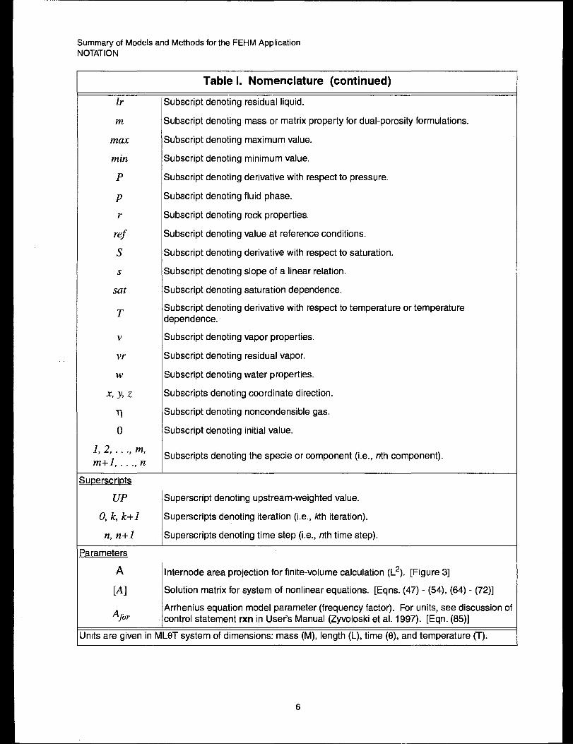
Table L Nomenclature (continued)
h- Subscript denoting residual liquid.
m Subscript denoting mass or matrix property for dual-porosity formulations.
max Subscript denoting maximum value.
min Subscript denoting minimum value.
P Subscript denoting derivative with respect to pressure.
P Subscript denoting fluid phase.
r Subscript denoting rock properties.
ref Subscript denoting value at reference conditions.
s Subscript denoting derivative with respect to saturation.
s Subscript denoting slope of a linear relation.
sat Subscript denoting saturation dependence.
TSubscript denoting derivative with respect to temperature or temperaturedependence.
v Subscript denoting vapor properties.
W Subscript denoting residual vapor.
w Subscript denoting water properties.
4 y, z Subscripts denoting coordinate direction.
~ Subscript denoting noncondensible gas.
o Subscript denoting initial value.
1,2, . . ..m.Subscripts denoting the specie or component (i.e., nth component).
m+l 9 ..., n
;uDerscri~ts
UP Superscript denoting upstream-weighted value.
O, k, k+l Superscripts denoting iteration (i.e., kth iteration).
n, n+l Superscripts denoting time step (i.e., nth time step).
‘arameters
A Internode area projection for finite-volume calculation (L*). [Figure 3]
[A] Solution matrix for system of nonlinear equations. [Eqns. (47) - (54), (64) - (72)]
‘forArrhenius equation model parameter (frequency factor). For units, see discussion ofcontrol statement rxn in User’s Manual (Zyvoloski et al. 1997). [Eqn. (85)]
Jnits are given in ML(3T system of dimensions: mass (M), length (L), time @), and temperature (T).
6
Summary of Models and Methods for the FEHM ApplicationNOTATION
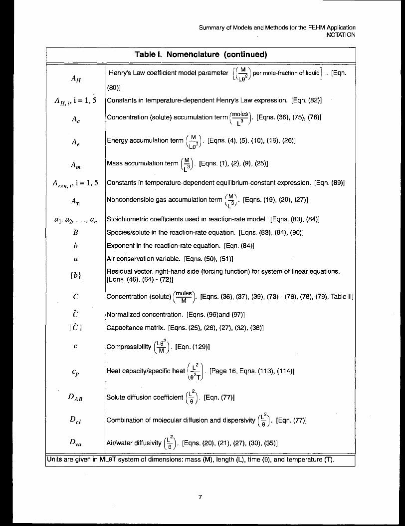
Table 1. Nomenclature (continued)
Henry’s Law coefficient model parameterM
AH [( )-@P 1er mole-fraction of liquid . [Eqn.
(80)]
AH, i,i=l,5 Constants h temperaiure-dependent Henry’s Law expression. [Eqn. (82)]
AC ()Concentration (solute) accumulation term - . [Eqns. (36), (75), (76)]
L’
A. Energy accumulation term():L . [Eqns. (4), (5), (10), (16), (26)]
Am ()Mass accumulation term ~ . [Eqns. (l), (2), (9), (25)]
A rxn, i Ti=l,5 Constants in temperature-dependent equilibrium-constant expression. [Eqn. (89)]
Aq ()Noncondensible gas accumulation term ~L . [Eqns. (19), (20), (27)]
al, az . . .. an Stoichiometric coefficients used in reaction-rate model. [Eqns. (83), (84)]
B Species/solute in the reaction-rate equation. [Eqns. (83), (84), (90)]
b Exponent in the reaction-rate equation. [Eqn. (84)]
a Air conservation variable. [Eqns. (50), (51)]
{b}Residual vector, right-hand side (forcing function) for system of linear equations.[Eqns. (46), (64) - (72)]
c()
Concentration (solute) Y . [Eqns. (36), (37), (39), (73) - (76), (78), (79), Table 11]
e Normalized concentration. [Eqns. (96)and (97)]
[c] Capacitance matrix. [Eqns. (25), (26), (27), (32), (36)]
c()
Compressibility ~ . [Eqn. (129)]
CP(1
Heat capacity/specific heat ‘2~T - [Page 16, Eqns. (1 13), (114)]
D AB()
Solute diffusion coefficient ~ . [Eqn. (77)]
Dcl0
Combination of molecular diffusion and dispersivity $ . [Eqn. (77)]
Dva()
Air/water diffusivity $ . [Eqns. (20), (21), (27), (30), (35)]
Jnits are given in ML6T system of dimensions: mass (M), length (L), time (6), and temperature (T).
7
Summary of Models and Methods for the FEHM ApplicationNOTATION
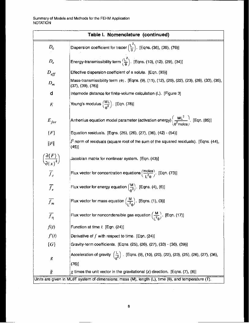
Table L Nomenclature (continued)
DC(1
Dispersion coefficient for tracer $ . [Eqns. (36), (38), (76)]
De()
Energy-transmissibility term $ . [Eqns. (10), (12), (29), (34)]
D effEffective dispersion coefficient of a solute. [Eqn. (93)]
D.Mass-transmissibility term (e). [Eqns. (9), (11), (12), (20), (22), (23), (28), (33), (35),
(37), (39), (76)]
d Internode distance for finite-volume calculation (L). [Figure 3]
E ()Young’s modulus ~L . [Eqn. (78)]
e
‘for()
Arrhenius equation model parameter (activation energy) ~ . [Eqn. (85)](32moles
{F} Equation residuals. [Eqns. (25), (26), (27), (36), (42) - (54)]
/]F/l ~ norm of residuals (square root of the sum of the squared residuals). [Eqns. (44),(45)]
d{F}
()Jacobian matrix for nonlinear system. [Eqn. (43)]
a{x]k
z ()Fiux vector for concentration equations %~ ~ . [Eqn. (73)]
z ()Flux vector for energy equation ~ . [Eqns. (4), (6)]
e
f. Flux vector for mass equation()& . [Eqns. (l), (3)]
~ Flux vector for noncondensible gas equation()& . [Eqn. (17)]
f(t) Function at time t. [Eqn. (24)]
f’(t) Derivative of ~ with respect to time. [Eqn. (24)]
{G} Gravity-term coefficients. [Eqns. (25), (26), (27), (33) - (36), (39)]
()Acceleration of gravity ~ . [Eqns. (9), (10), (20), (22), (23), (25), (26), (27), (36),
s e
(76)]
E g times the unit vector in the gravitational (z) direction. [Eqns. (7), (8)]
Jnits are given in MLeT system of dimensions: mass (M), length (L), time (e), and temperature (T).
8
Summary of Models and Methods for the FEHM ApplicationNOTATION
Table L Nomenclature (continued)
AHH()
Henry’s Law-equation model parameter (heat of reaction) * . [Eqn. (80)]ezmoles
AH,xn[)
Equilibrium-constant model parameter (heat of reaction) ~ . [Eqn. (87)]82moles
h[1
Enthalpy $ . [Eqns. (6), (12), (13), (62), (63),(113),(1 15),(116)]
Im ()Mass-flow impedance ~ . [Eqn. (40)]
1, Heat-flow impedance()&T . [Eqn. (41)]
K ()Thermal conductivity ~~ . [Eqns. (6), (16), (26), (31), (133), (134), Page 21]
T8
Kd Retardation coefficient (linear adsorption). ~able Ii]
K,q Equilibrium constant. [Eqns. (86) - (89)]
K eq, 25 Equilibrium constant at 25°C. [Eqn. (87)]
Keq Intermediate term used in equilibrium constant expression. [Eqns. (88) and (89)]
‘fact Multiplier to increase reaction rates to approach equilibrium behavior.
KH Henry’s Law constant (!$) [Eqn. (1 18)1, [(’) per mole-fraction of liquid] [Eqn. (80)].
& Intermediate term used in expression of Henry’s Law constant. [Eqn. (82)]
k~ Intermediate term used in expression of Henry’s Law constant. [Eqn. (82)]
k Intrinsic rock permeability (L*). [Eqns. (7), (8), (11), (61), (62), (63), (132)]
‘for’ ‘rev Forward and reverse reaction rate constants. [Eqns. (84), (85)]
kRn Radioactive-decay rate constant, [Eqn. (102)]
L Flow path length (L).
Length scales used in dual-porosity and double-porosity/double-permeabilityLf Lfl LP~ Ljz problems. [Eqns. (56), (58), (59), (60), Figure 4]
M ()Molecular weight ~ . [Eqn. (79)]
‘fFluid mass in a cell (M). [Eqn. (91)]
m Exponent used in Gangi stress model. [Eqn. (130)]
Jnits are given in MLf3T system of dimensions: mass (M), length (L), time @), and temperature (T).
9
Summary of Models and Methods for the FEHM ApplicationNOTATION
Table 1. Nomenclature (continued)
mout()
Outlet mass flow rate from one cell to another ~ . [Eqn. (91)]
Experimental parameter used in van Genuchten relative-permeability and capillary-n
pressure models. [Page 57, Page 58]
[M Finite-element shape function. [Page 20, Eqns. (28) - (34), (37) - (39)]
()Pressure ~ .
P[Eqns. (7) - (10), (20), (22), (23), (25), (26), (27), (36), (40), (47) -
(54), (61), ;2), (63), (76), (79), (104) - (107),(1 11),(1 18), (127) - (129), (131)]
Pc Closure stress for use in Gangi stress model (ML). [Eqns. (130), (131)]
Pe Peclet number for dispersion. [Eqns. (96) and (97)]
q. ()Concentration source term - . [Eqns. (36), (74), (76)]
L%
q. ()Energy source term ~ . [Eqns. (4), (10), (13), (16), (26), (41)]
L(33
Solute flux term from fracture to matrix in particle-tracking model development.qfm [Eqn. (99)]
qrn ()Mass source term & . [Eqns. (l), (9), (14), (22), (23), (25), (40)]
qllNoncondensible gas source term
()~ . [Eqns. (18), (20), (27)]
R Universal gas constant (8.31 4 kJ/mol-K). [Eqns. (80), (85), (1 10)]
‘fSorption retardation factor. [Eqn. (92)]
Rp Relative permeability. [Eqns. (7), (8), (11), (15), (121) -(1 26)]
~ rb Parameters used in nonlinear adsorption model (Langmuir). Table l!]
s Saturation. [Eqns. (2), (5), (19), (22), (23), (53) - (54), (121) - (128)]
TTemperature (T). [Eqns. (6),(16), (41), (47), (48), (50) - (52), (80), (85),(104) -(1 07),
(111), (113), (114), (131)]
[n Stiffness matrix. [Eqns. (25) - (29), (36), (37)]
T’ ~Tflj2 Transfer terms in dual-porosity solution. [Eqns. (59) - (63)]
t Time (e). [Eqns. (1), (4), (9), (1O), (16), (20) - (27), (36), (76)]
u[1
Internal energy $ . [Eqn. (5)]
v Integral volume. [Eqns. (28) - (34), (37) - (39)]
Jnits are given in MLeT system of dimensions: mass (M), length (L), time (El), and temperature (T).
10
Summary of Models and Methods for the FEHM ApplicationNOTATION
Table L Nomenclature (continued)
v’
Vfl Vp, vj’2
VT
v
7
Vl,x
w
x
{x}
2
Y
z
z
a
al, (X2
c(~
cx~
P
7rxn
Ttol
&
n
e
6
A
Volume fraction for fractures in dual-porosity and double-porosity/double-permeabilityproblems. [Eqns. (55) - (58)]
Volume fractions for the matrix volumes used in dual-porosity and double-porosity/double-permeability problems. [Eqns. (55) - (58)]
Total volume of computational cell (L3). [Eqn. (59), (60)]
Superficial velocity in one-dimensional model used in particle-tracking modeldevelopment. [Eqn. (93)]
()Velocity vector ~ . [Eqns. (3), (6) - (8), (17)]
Darcy velocity of liquid phase, x-direction. [Eqn. (77)]
Weighting factor for time discretization. [Eqn. (24)]
Pressure or temperature variable in rational-function approximation for saturationequations. [Eqns. (108), (109)]
Solution vector. [Eqns. (42), (43), (46), (64) - (72)]
Normalized distance along flow path. [Eqn. (96)]
Polynomial in numerator of rational-function approximation. [Eqns. (1 04) -(1 09)]
Polynomial in denominator of rational-function approximation. [Eqns. (104) -(1 09)]
Coordinate oriented in the direction of gravity. [Eqns. (9), (10), (20), (33), (34), (39), (76)
()Coefficient of thermal expansion ~ . [Eqn.(131 )]
Coefficients used in sorption models. [Eqns. (78), (90), Table 11]
Dispersivity of solute in transport calculations (L) .
Experimental parameter used in van Genuchten capillary-pressure model. [Page 58
Exponent used in sorption models. [Eqns. (78), (90), Table 11]
Fractional approach to equilibrium computed at an iteration in the reactive-transportmodel. [Eqn. (91)]
Fractional approach to equilibrium specified for an equilibrium reaction. [Eqn. (91)]
lTolerance taken for solution scheme. [Eqn. (45)]
Mass fraction of air. [Eqns. (2), (3), (9), (17) - (20), (27), (35), (1 15) -(1 19)]
Exponent used in the air/water diffusion model. [Eqn. (21)]
Normalized time. [Eqns. (96)and (97)]
Parameter used in nonlinear adsorption model (Freundlich, modified Freundlich).~able 11]
I
Jnits are given in MLeT system of dimensions: mass (M), length (L), time (6), and temperature (T).
11

Summary of Models and Methods for the FEHM ApplicationSTATEMENT AND DESCRIPTION OF THE PROBLEM
I
II
I
Table 1. Nomenclature (continued)
AParameter used in van Genuchten relative-permeability and capillary-pressuremodels. [Eqn. (125), Page 58]
P ()Viscosity # . [Eqns. (7), (8),(1 1), (15), (61), (62), (63),(1 19), (120)]
v Fractional vapor flow parameter. [Eqns. (14), (15)]
()Density fi . [Eqns. (3), (5), (7) -(1 1), (15), (17), (19) - (23), (61), (62), (63), (76),
P(90), (111), (112), (117) ]
/n ~itu stress ~L0
()[Eqn. (131)]
(32 -
T Tortuosity factor in the air/water diffusion model. [Eqn. (21)]
‘t age Particle age since entering the model domain (6). [Eqn. (102)]
Tf Fluid residence time in a cell (0). [Eqn. (91)]
‘part Particle residence time in a cell (0). [Eqn. (91)]
71/2 Radioactive-decay half-life (8).
o Porosity. [Eqns. (2), (5), (19), (21) - (23), (90), (129), (130), (132)]
~mal Matrix porosity in particle-tracking model. [Eqn. (99)]
Q Flow domain of the model. [Eqns. (28) - (34), (37) - (39)]
Jnits are given in ML(3T system of dimensions: mass (M), length (L), time (13),and temperature (T).
5.0 STATEMENT AND DESCRIPTION OF THE PROBLEM
The primary use of the FEHM application will be to assist in the understanding of flow
fields and mass transport in the saturated and unsaturated zones below the potential
Yucca Mountain repository. Studies in the saturated zone are prescribed in YMP-
LANL-SP-8.3 .1.2 .3.1.7 (the C-Wells project) and include use of the FEHM code to design
and analyze tracer tests (reactive and nonreactive) to characterize the flow field below
Yucca Mountain. Studies in the unsaturated zone are prescribed in YMP-LANL-SP-
8.3.1 .3.7.1 and include the study of coupled processes (multicomponent flow and natural
convection).
Yucca Mountain is extremely complex both hydrologically and geologically. The
computer codes that are used to model flow must be able to describe that complexity.
For example, the flow at Yucca Mountain, in both the saturated and unsaturated zones
is dominated by fracture and fault flow in many areas. With permeation to and from
faults and fractures, the flow is inherently three-dimensional (3-D). Birdsell et al.
(1990) presented calculations showing the importance of 3-D flow at Yucca Mountain.Coupled heat and mass transport occurs in both the unsaturated and saturated zones.
In the near-field region surrounding the repository, the coupled flow effects dominate
the fluid behavior. Here, boiling, dryout, and condensation can occur (Nitao 1988). In
12

Summary of Models and Methods for the FEHM ApplicationSTRUCTURE OF THE SYSTEM MODEL
6.0
the far-field unsaturated zone, Weeks (1987) has described natural convection that
occurs through Yucca Mountain due to seasonal temperature changes. Heat and mass
transfer are also important in matching saturated-zone models to temperature logs and
pressure tests and in modeling enhanced convection due to repository heating.
The transport processes at Yucca Mountain are very complex. Various adsorption
mechanisms ranging from simple linear relations to nonlinear isotherms must be
incorporated in the transport models. Multiple interacting chemical species must be
modeled so that this structure can represent radioactive decay with daughter products
and coupled geochemical transport.
STRUCTURE OF THE SYSTEM MODEL
The component models that make up the overall transport model are:
Flow- and Energy-Transport Equations for simulation of processes within porous
and permeable media, which include:
. heat conduction only;
. heat and mass transfer with pressure- and temperature-dependent
properties, relative permeabilities, and capillary pressures;
. isothermal air-water transport; and
● heat and mass transfer with noncondensible gas.
Dual-Porosity and Double-Porosity/Double-Permeability Formulation for problems
dominated by fracture flow.
Solute-Transport Models, including:
. a reactive-transport model that simulates transport of multiple solutes with
chemical reaction; and
● a particle-tracking model.
Constitutive Relationships for pressure- and temperature-dependent fluid/air/gas
properties, relative permeabilities and capillary pressures, stress dependencies,
and reactive and sorbing solutes, which encompass:
s thermodynamic equations;
. air and airlwat er vapor mixtures;
s equation-of-state models;
● relative-permeability and capillary-pressure functions;
● stress-dependent properties; and
● variable thermal conductivity.
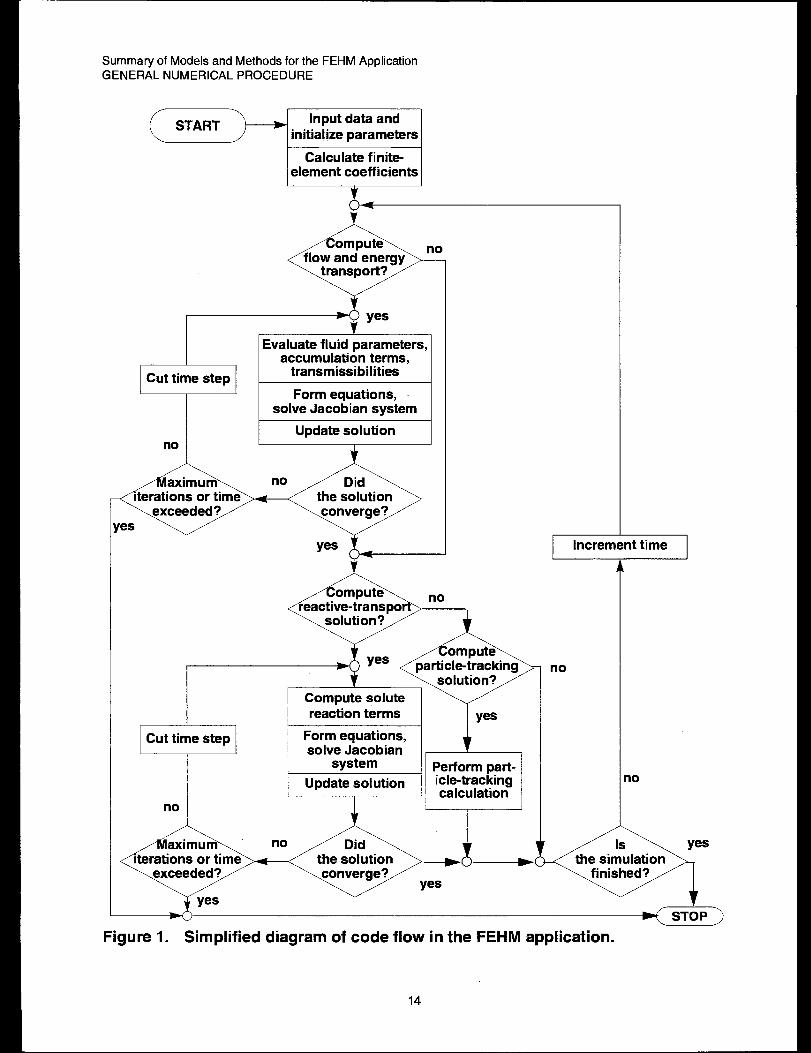
7.0 GENERAL NUMERICAL PROCEDURE
The numerical solution strategy for FEHM is shown in Figure 1.
13
Summary of Models and Methods for the FEHM ApplicationGENERAL NUMERICAL PROCEDURE
Input data andinitialize parameters
IF===
TnoUpdate solution I
Cut time step
no
oompute noreactive-transpo —
solution?
L
yes
‘5(\ompute
particle-trackingsolution?
Compute solutereaction terms yes
Form equations,solve Jacobian
system
n
Perform part-Update solution icle-tracking
calculation
‘J’yes
I Increment time
no
IoIs yesthe simulation
finished?
1
Figure 1. Simplified diagram of code flow in the FEHM application.
14

Summary of Models and Methods for the FEHM ApplicationCOMPONENT MODELS
8.0 COMPONENT MODELS
8.1 Flow and Energy-Transport Equations
8.1.1
8.1.2
8.1.3
Purpose
The purpose of this model is to simulate heat conduction, heat and mass
transfer for multiphase flow within porous and permeable media, and
noncondensible gas flow within porous and permeable media.
For heat conduction, the input to the model consists of an initial
description of the media (rock) properties and state. The output consists of
a final media state.
For heat and mass transfer, the input to the model consists of an initial
description of the fluid state as well as media properties. The output
consists of the final fluid and media states.
For noncondensible gas flow, in addition to the initial media properties and
fluid state, the description of the initial state of the gas is required. The
output consists of the final state of the gas in addition to that described for
the previous components.
Assumptions and limitations
The major assumptions are those associated with Darcy’s law for fluid flow.
This restriction means the velocity of fluid flow must be very slow. The
exact quantification of the values is best addressed in the associated
validation report (Dash et al. 1997). Another assumption is thermal
equilibrium between fluid and rock (locally), which is usually an excellent
assumption as the thermal wave for rocks travels on the order of 10-3 m/s,
10-3 m is the upper limit of the pore size, and fluid velocities are of the
order of 10-5 mis.
Other assumptions include an immovable rock phase and negligible viscous
heating. The assumptions associated with flow are discussed in Brownell,
et al. (1975).
Derivation
Because the derivations of the governing equations are analogous for heat
conduction, heat and mass transfer for multiphase flow within porous and
permeable media, noncondensible gas flow within porous and permeable
media, and transport of multiple solutes within porous and permeable
media, only the heat and mass derivation will be presented.
Detailed derivations of the governing equations for two-phase flow
including heat transfer have been presented by several investigators (e.g.,
Mercer and Faust 1975; Brownell et al. 1975), therefore, only a brief
development will be presented. The notation used is given in Table I.
Conservation of mass for water is expressed by the equation
15
Summary of Models and Methods for the FEHM ApplicationCOMPONENT MODELS
3A. —
at_+v. fm+qm=o, (1)
where the mass per unit volume, Am, is given by
(2)Am = $(svpv(l -q,)+ ~lPz(l -TI1))
and the mass flux, f—~,is given by
~ = (l- Tlv)Pvi+(PTIJP~i - (3)
Here, @ is the porosity of the matrix, S is saturation, p is density, v is the
concentration of the noncondensible gas and is expressed as a fraction of
the total mass, 7 is velocity, and the subscripts v and 1 indicate quantities
for the vapor phase and the liquid phase, respectively. Source and sink
terms (such as bores, reinfection wells, or groundwater recharge) are
represented by the term qm.
Conservation of fluid-rock energy is expressed by the equation
aAe – –
at—+v. fe+qe= c)? (4)
where the energy per unit volume, Ae, is given by
(5)Ae = (1 – @)PrZZr+ $(~VPVUV + ~lPzz@ ~
—with Ur = cprT, and the energy flux, f~, is given by
~ = pVhV< + plhl<-K~T . (6)
Here, the subscript r refers to the rock matrix, Ur, UV,and U1are specific
internal energies, Cpr is the specific heat, hv and hz are specific enthalpies, K
is an effective thermal conductivity, T is the temperature, and q= is the
energy contributed from sources and sinks.
To complete the governing equations, it is assumed that Darcy’s Law
applies to the movement of each phase:
— kRv _Vv = ----(VPv - pvg)
and
16
(7)
(8)
Summary of Models and Methods for the FEHM ApplicationCOMPONENT MODELS
Here, k is the permeability, RV and Rz are the relative permeabilities, WV
and pz are viscosities, PV and P1 are the phase pressures, and g represents
the acceleration due to gravity (the phase pressures are related by
Pv = Pl + Pcap, where PCap is the capillary pressure). For simplicity, the
equations are shown for an isotropic medium, though this restriction does
not exist in the computer code.
Using Darcy’s Law, the basic conservation equations, (1) through (4), can
be combined:
-v“ ((1 –nv)DmvvPv) – v “((1 –Tll)DmlvP1) + qm+
(9)
and
–v“ (DevvPv) - v “(DelvP1) - v “(Km)+ qe +
dAe(lo)@l?vPv + ~.lPJ + -=&- = 0,
where z is oriented in the direction of gravity. Here, the transmissibilities
are given by
kRVpV ‘%P1D=mv —, Dml=—
P’v l-+(11)
and
De, = hvDmv , Del = hlDml . (12]
The source and sink terms in Eqns. (1) and (4) arise from bores, and if the
total mass withdrawal, qm, for each bore is specified, then the energy
withdrawal, qe, is determined as follows:
q, = (#q+ qlhl , (13)
where
qv = Vqm ,q~ = (l-v)qm , (14)
and
(15)
17

Summary of Models and Methods for the FEHM ApplicationCOMPONENT MODELS
The form of Eqn. (15) shows how important the relative permeability ratio
Rz /RV is in controlling the discharge composition. Other source/sink terms
arise from implementation of boundary conditions. These include specified
pressure and temperatures and are discussed in the “Boundary conditions”
subsection of Section 8.1.6, “Derivation of numerical model”. The relative-
permeability and capillary-pressure functions are summarized in Section
8.4, “Constitutive Relationships”.
The final form of the pure heat-conduction equation is easily obtained from
Eqn. (10) when all convective terms are eliminated:
i3A–V. (m)+qe+z’=o (16)
The mass flux, ~n, source (or sink) strength, qq, and accumulation term,
An, are defined as follows for the noncondensible gas conservation
equation:
A?l= WLJVPV + %ql) “
The noncondensible gas conservation equation is
-v“ (T-@my’v)- v“ (Ipmlm’l)- v“ (Dvav?-lv)+ qn +
~A&lv%vPv + ‘w~m~Pl) + & = 0.
(17)
(18)
(19)
(20)
Here, ?l is the concentration of the noncondensible gas and is expressed as
a fraction of the total mass. As with the water-balance equations, source/
sink terms are used to implement boundary conditions. The reader is
referred to the ‘Boundary Conditions” subsection of Section 8.1.6,
“Derivation of numerical model”, for details.
The air/water diffusivity (Pruess 1991) is given by
Do 0.101325 T+ 273.15 e= Z$SVDVaPV p
vu[ 1273.15 ‘
(21)
where T is the tortuosity factor and D~a is the value of Dva at standard
conditions. Within FEHM, the value of llVa is set to 2.4 x 10⁻⁵ m2/s, () is set
to 2.334, and the tortuosity factor is an input parameter.
18

Summary of Models and Methods for the FEHM ApplicationCOMPONENT MODELS
8.1.4
Equations (9), (10), (16), and (20) represent the model equations for fluid
and energy transport in the computer code FEHM. It should be noted that
Eqn. (9) with q set to O also represents pure water.
For situations in which heat effects are minimal, the model can be
simplified. The isothermal air-water two-phase system in FEHM is
represented somewhat differently than the nonisothermal system defined
above. Here, the liquid phase is pure water and the vapor phase is pure
air. The component mass-balance equations are then also phase-balance
equations:
(22)
(23)
where Eqn. (22) is the water-balance equation and Eqn. (23) refers to the
conservation of air. Here, the subscript 1 refers to the liquid-water
properties and v refers to air properties. One option in the model is to
solve Eqns. (22) and (23) as a full two-phase flow problem. A further
simplification can be made in which the air pressure is assumed to be
constant. This assumption leads to an equation that is similar to
Richard’s equation for unsaturated flow. The method reduces to using only
Eqn. (22). The method is described further in the subsection on “Reduced
degree-of-freedom algorithms” in Section 8.1.6.
Applications
The component model described above may be used to model the flow of air,
water, water vapor, and heat in a porous medium. The validity of the
model is dependent on the validity of the equations described in
Section 8.1.3. The flow of both air and water must be sufficiently small at
all possible flow rates so that the above described equations will be valid.
This restriction is believed to be satisfied at Yucca Mountain. Of more
concern is the accuracy of the required input and the numerical precision to
which these equations are solved.
For the flow equations, the saturated permeabilities, porosities, fracture
permeabilities, and volumes of hydrogeologic units are required. In
addition, the relative-permeability and capillary-pressure functions are
required. Historically this information has been difficult to obtain. It is
important to note that the capillary pressure at low liquid saturations is
very important to the validity of the calculations but is not available in
regions near the residual saturations.
The issue of numerical accuracy is extremely important to the usefulness of
the results. The accuracy may be evaluated by solving the same problem
using different size grids and evaluating the change in the solution.

Summary of Models and Methods for the FEHM ApplicationCOMPONENT MODELS
8.1.5
8.1.6
Numerical method type
The primary numerical method used in FEHM is the finite-element
method. The reader is referred to Zienkiewicz (1977) for an excellent
account of this method. The summary of the numerics in FEHM given
Section 8.1.6 assumes a basic knowledge of the numerical solution of
in
partial differential equations. In addition, a working knowledge of the
finite-element method is helpful.
Derivation of numerical model
Discretization. The time derivatives in Eqns. (9), (10), (16), (20), and (76)
are discretized using the standard first-order method (Hinton and Owen
1979) given by
f(fn+1,= f(tn)+At[w~’(tn+ 1) + ( 1- W) fl’(tn)] , (24)
where ~(t” + 1) is the desired function at time t“+ 1,f(t”) is the known
value off at time t“, At is the time step, f“ is the derivative of f with
respect to time, and w is a weighting factor. For w = 1 , the scheme is
fully implicit (backward Euler), and for w = O, the scheme is fully explicit
(forward Euler).
The space derivatives in the governing equations are discretized using the
finite-element formulation. The finite-element equations are generated
using the Galerkin formulation. For a detailed presentation of the finite-
element method, the reader is referred to Zienkiewicz (1977). In this
method, the flow domain, ~, is assumed to be divided into finite elements,
and variables P, T, and ?l, along with the accumulation terms Am, Ae, and
Aq, are interpolated in each element: PV = [N] {P,}, P1 = [N] {Pl} ,
T = [N]{ T}, q, = [iV]{qV}, Am = [ZV]{Am}, Ae = [N]{Ae}, and
An = [N]{ An } , where [N] is the shape function.
These approximations are introduced in Eqns. (9), (10), (16), and (20), and
the Galerkin formulation (described by Zienkiewicz and Parekh 1973) is
applied. The following equations are derived:
{1dA[Tm,.l{p.}+ U’m,ll{pl}+ [~1 ~m +{qm}-
g{~m, vl-g{Gm,lJ = {Fml ,
{}
aA[T.,,]{%} + [Te,ll{pl} + [~l{T} + [?] =’ +
{~el-g{Ge, vJ-g{Ge,l) = {Fe} ,
and
(25)
(26)
20
Summary of Models and Methods for the FEHM ApplicationCOMPONENT MODELS
{1i3A[qvlu’v} + W?lll{w + [~val{’w} + m # +
{qq}-g{Gq,.}-Wq,[l = W’ql Y (27)
where
(28)
!2
‘p ~NjdV ,Teij = ~~Ni. De (29)
L2
(30)
~ij = ~NiNj dV , (32)
a
dNiGmi = ~zNj D:p pm dV ,
S1
‘~e dV .
(33)
(34)
dNi(35)‘~i = J’ ~NjD.T
L2
2KiKjIn the above equations, ~ =
UP
K;+K,and the D terms indicate an
upstream-weighted transmissibility (Dalen 1979). This technique has
worked well in the low-order elements (3-node triangle, 4-node
quadrilateral) for which the schemes resemble difference techniques. The
upstream weighting is determined by evaluating the internode flux for the
nodes i and ~. The shape-function coefficients are generated in a unique
way that requires the integrations in Eqns. (33), (34), and (35) to be
performed only once and the nonlinear coefficients to be separated from
this integration (see Zyvoloski 1983 for more details).
The integration schemes available in FEHM are Gauss integration and a
node-point scheme used by Young (1981). His implementation differs from
common methods in that it uses Lobatto instead of Gauss integration. The
21

Summary of Models and Methods for the FEHM ApplicationCOMPONENT MODELS
net effect is that, while retaining the same order of integration accuracy (at
least for linear and quadratic elements), there are considerably fewer
nonzero terms in the resulting matrix equations. Figure 2 shows a
comparison of the nodal connections for Lobatto and Gauss integration
methods. It should be noted that these results hold on an orthogona grid
0’ IA I
—
Figure 2. Comparison of nodal connections for conventional (o)
and Lobatto (o) integrations for an orthogonal grid.
only. If a nonorthogonal grid were introduced, then additional nonzero
terms would appear in the Lobatto quadrature method. Note also that the
linear elements yield the standard 5- or 7-point difference scheme. The
reader is referred to Young (1981) for more details.
In addition to the finite-element integration techniques described above,
the code has provisions for finite-volume calculation of the internode flow
terms described by Eqns. (28) to (35). In the finite-volume approach, the
geometric terms are calculated as area projections and distances between
nodes. The geometric part of Eqns. (28), (29), and (30) are given by the
area between the nodes divided by the distance. The area is partitioned
according to the perpendicular bisectors of the midpoints of the sides of the
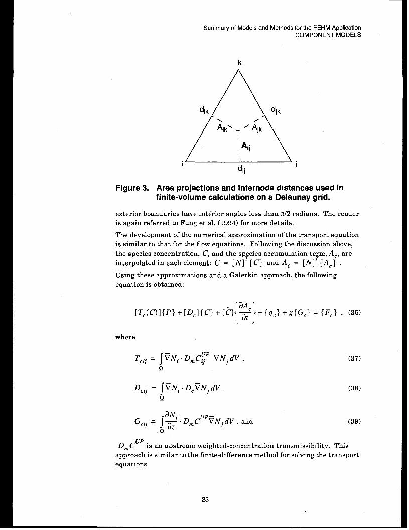
elements. This technique is shown in Fig. 3 for triangles in two
dimensions. An analogous approach is used in three dimensions for
tetrahedral. Quadrilaterals in two dimensions and hexahedrals in three
dimensions are first decomposed into triangles and tetrahedrals,
respectively, and the geometry coefficients formed as described above. For
more details the reader is referred to Fung et al. (1994).
It is important to note here that with upwinding, the geometric factors that
govern internode flow, regardless of whether calculated from a finite-
element or finite-volume approach, must not change in sign. This requires
a Delaunay grid plus the constraint that any elements at interfaces or
22
Summary of Models and Methods for the FEHM ApplicationCOMPONENT MODELS
k
Figure 3. Area projections and internode distances used infinite-volume calculations on a Delaunay grid.
exterior boundaries have interior angles less than z/2 radians. The reader
is again referred to Fung et al. (1994) for more details.
The development of the numerical approximation of the transport equation
is similar to that for the flow equations. Following the discussion above,
the species concentration, C, and the sp~cies accumulation te~m, AC, are
interpolated in each element: C = [N] {C} and AC = [N] {AC} .
Using these approximations and a Galerkin approach, the following
equation is obtained:
[Tc(c)]{l’} + [Dc]{c} + [t]{1‘+ +{qc}+g{Gc} = {Fc} , (36)
where
dNiGcij = ~~ . DmCup~Nj dV , and
n
(37)
(38)
(39)
DmCup is an upstream weighted-concentration transmissibility. This
approach is similar to the finite-difference method for solving the transport
equations.
23

Summary of Models and Methods for the FEHM ApplicationCOMPONENT MODELS
Boundary conditions. Two types of fluid (mass) sources and sinks are
implemented: a specified flow-rate source/sink and a specified pressure
condition at a source/sink. No-flow or impermeable boundary conditions
are automatically satisfied by the finite-element mesh. The constant-
pressure boundary condition is implemented using a pressure-dependent
flow term:
q = L, iu’ji!ow,~– ~J 2m, i (40:
where Pi is the pressure at the source node i, PflOw,i is the specified flowing
pressure, Im, i is the impedance, and qm, i is the mass flow rate. By
specifying a large I, the pressure can be forced to be equal to PflOw. The
energy (temperature) specified at a source/sink or flowing pressure node
refers only to the incoming fluid value; if fluid flows out, stability dictates
that the energy of the in-place fluid be used in calculations.
In addition to the mass-flow source/sink, heat-flow sources can also be
provided. A specified heat flow can be input or a specified temperature
obtained:
(? - ‘e, i( ‘flow, 1e,i — -Ti) , (41)
where Ti is the temperature at the source node i, TflOw,i is the specified
flowing temperature, le,i is the impedance to heat flow (thermal
resistance), and qe, i is the heat flow. This heat flow is superimposed on
any existing heat flow from other boundary conditions or source terms.
Specified saturations, relative humidities, air-mass fractions, as well as
specified air flows are allowed. These use source/sinks to achieve the
desired variable values in a way that is analogous to that described for
pressure boundary conditions.
In FEHM, there is also a provision for creating large volume reservoirs
that effectively hold variables at their initial values. The nodes are labeled
on input and the volumes replaced after the calculation of the geometric
coefficients with a reservoir volume of 1013 m3.
Solution method. The application of the discretization methods to the
governing partial differential equations yields a system of nonlinear
algebraic equations. To solve these equations, the Newton-Raphson
iterative procedure is used. This iterative procedure makes use of the
derivative information to obtain an updated solution from an initial guess.
Let the set equations to be solved be given by
{F}({x}) = {o} , (42)
where {x} is the vector of unknown values of the variables that satisfy the
above equation. ‘$he procedure is started by making an initial guess at the
solution, say {x} . This guess is usually taken as the solution from the
24
previous time step. Denoting the value of {x} at the kth iteration by
{x} , the updating procedure is given by
{x}k+l =k il{F} ‘1{X}k - {F} (a{x}k
)(43)
At each step, the residuals {F}k = { F}({ X}k) are compared with a
prescribed error tolerance. The prescribed error tolerance, &, is an input
parameter, and an 12 norm is used:
llF/]k= (~F:)l’2 .i k
Convergence is achieved when
(44)
(45)
The value of& is usually in the range from 10-4 to 10-7. Semiautomatic
time-step control is designed based on the convergencekof the Newton
iterations. If the code is unable to find a solution {x} such that the
residuals become less than the tolerance within a given number of
iterations, the time step is reduced and the procedure repeated. On the
other hand, if convergence is rapid, the time step is increased by
multiplying with a user-supplied factor, thus allowing for large time steps
when possible.
The linear equation set to be solved at each Newton-Raphson iteration of
Eqn. (43) is
a{F} {Ax}k+l = -{F}k ,()a{x}k
a{F}
()where — is the Jacobian matrix, {Ax }k + 1
a~x]kis the change in the
(46)
. .k+l k+l k
solution vector {Ax = x – x }, and { F}k is the residual.
It is solved with a reuse component, GZSOLVE (see Zyvoloski and Robinson
1995), that provides a robust solution method for sparse systems of
equations. Further details of the solution procedure can be found in the
GZSOLVE MMS component of the document just cited.
Reduced degree-of-freedom algorithms. In the coupled physical
processes that describe flow in porous media, one process is often
dominant. In heat and fluid flow, for example, the pressure changes more
rapidly than the temperature. As recognized by Zyvoloski et al. (1979),
this fact may be used to simplify the linear equations solved at each step of
a Newton-Raphson iteration. Solving the pure-water heat and mass flow
leads to the following set of linear equations at each such iteration:
25
Summary of Models and Methods for the FEHM ApplicationCOMPONENT MODELS
Fm
Fe(47)
The subscripts m and e refer to the mass- and energy-balance equations,
respectively. The subscripts P and T refer to derivatives with respect to
pressure and temperature, respectively. The superscripts indicating the
iteration number have been dropped for convenience. From Eqns. (9) and
(10), it can be seen that the primary contribution of temperature is to affect
the thermal conduction terms and the density and viscosities. Pressure,
however, affects the density and is directly involved in the Darcy velocities.
In other words, the pressure more directly affects the global transport of
heat and mass. Guided by this reasoning, a computationally efficient
scheme is obtained by neglecting the off-diagonal derivatives with respect
to temperature. With this modification, we can solve for the temperature
change using:
{AT} = [AeJ1{-{Fe} - [Aepl{Ap}} . (48)
This result may, in turn, be substituted in the mass-balance portion of
Eqn. (47) giving:
[[Ampl - [& Tl[AeT1-l [Aep: I{AP}=
- {Fm} + [AmT] [Ae~]-” {Fe} . (49)
The indicated matrix inversions and multiplications are performed with
diagonal matrices, and the resulting matrix for the calculation of the
pressure correction is a banded matrix of exactly the same structure as
[Amp] . It was found that additional efficiency could be achieved by taking
several passes of SOR (simultaneous over-relaxation) iterations after the
system in Eqns. (48) and (49) was solved (Bullivant and Zyvoloski 1990).
The same process can be used to reduce the air/water/heat-coupled system
to a one or two degree-of-freedom problem. The coupled 3n by 3n system
may be written as
]{
Amp A~~ Ama Ap
A,p A,~ Aea AT
Aap Aa~ Aaa Aa
=—
Fm
Fe
F.
(50)
26
Summary of Models and Methods for the FEHM ApplicationCOMPONENT MODELS
Here, the subscript a refers to the conservation of air mass and derivatives
with respect to the air variable. The air variable is eliminated in favor of
the pressure and temperature using
{As} = [Aaal-l{-{Fa} - [Aap]{AI’} - [A, TI{AT} } . (51)
Substituting this in the mass- and energy-correction equations yields:
1[[AmTl - [Amal[Aaal-l[AaTll { AP ]
[
[[Ampl - [Amal[Aaal-l [Aapll
[[Aepl - [&JIAaal-l[Aapll [[AeTl - [&J[&J-l[AaTllj [ ‘T J
!
- {Fm} + [Ama][Aaa]-l{Fa}=
- {Fe} + [Aea][Aaa]-l{Fa}
(52)
During the simulation, the phase state of the system can change. This
possibility makes it necessary to rearrange Eqns. (51) and (52). The
method remains the same. The reduced Eqns. (51) and (52) are useful in
thermal simulations in which phase changes or other factors reduce the
time step. The 3n-by-3n system may further be reduced to an n-by-n
system (discussed in Bullivant and Zyvoloski ‘1990). Bullivant and
Zyvoloski also showed that the operations given above can conveniently be
done during the equation normalization process.
The last reduced degree-of-freedom algorithm to be described reduces the
isothermal air/water problem to a one-variable system. The result is
similar to the Richard’s solution. To obtain a computationally efllcient
scheme, the air pressure is constrained to atmospheric pressure in the two-
phase region and the liquid saturation is constrained to 1.0 in the one-
phase liquid region. The method involves switching variables and
associated derivatives in the solution of the linear system that produces
the Newton-Raphson correction. The matrix equation that describes the
Jacobian matrices for an isothermal system is given by
[AWPI{AP} + [AWJ{AS} = -{Fw} . (53)
Here, the subscript w refers to the water-conservation equation, and the
subscripts P and S refer to derivatives with respect to pressure and
saturation, respectively. Though Equation (53) has the appearance of
being underconstrained, for every matrix position there is only one nonzero
entry in the two matrices [Awp] and [Aw~] . This is a consequence of the
variable switching just discussed. The algorithm consists of replacing
terms in [Awp] with terms from [AWJ if two-phase conditions exist at a
node. The resulting system is given by

Summary of Models and Methods for the FEHM ApplicationCOMPONENT MODELS
8.2
8.1.7
8.1.8
8.1.9
[Awx]{x} = -{Fw} , (54)
where x represents pressure or saturation, depending on the nodal phase
state.
Location
The implementation sequence for the Flow- and Energy-Transport
Equations may be seen in Fig. 1 in which the box “Form equations, solve
Jacobian system” indicates the position in the algorithm of the components
of these equations in the overall structure of FEHM.
Numerical stability and accuracy
The equations that are solved are highly nonlinear and coupled. The
stability of the system has been maximized by solving the fully coupled and
fully implicit formulation of the problem. Because of the nonlinearity,
however, stability cannot be guaranteed. Logic has been incorporated to
restart a time step if the code realizes it is calculating in an area in which
the equation of state (as implemented by FEHM) is not valid.
Accuracy of the simulations is also clouded by the nonlinearity issue.
Formally, the spatial differencing is second-order accurate and the time
terms are first-order accurate. There is a provision (which is usually
invoked) that upwinds the transmissibility terms. This reduces the spatial
accuracy to first order. It is difficult in practice to estimate the quality of a
simulation from these theoretical considerations. The user is advised to
run a given problem with several grid sizes and time-step sizes to assess
the quality of a particular solution obtained with FEHM. The accuracy of
the calculations is also addressed in the FEHM verification report (Dash
and Zyvoloski 1997).
Alternatives
The primary alternative to the formulation given here is an integrated
finite-difference formulation. The reader is referred to Nitao (1988) and
Pruess (1991) for details. The basic difference in theory is that FEHM uses
a node-centered approach, whereas the integrated finite-difference
formulation uses a cell-centered approach. Classical finite differences may
also be used to solve the equations presented here, but this approach lacks
the geometric flexibility of the other methods mentioned.
Dual-Porosity and Double-Porosity/Double-PermeabilityFormulation
8.2.1 Purpose
Many problems are dominated by fracture flow. In these cases, the
fracture permeability controls the pressure communication in the reservoir
even though local storage around the fracture may be dominated by the
porous rock that communicates only with the closest fractures. This
phenomena requires a model in which the fractures dominate the global
28

Summary of Models and Methods for the FEHM ApplicationCOMPONENT MODELS
pressure response of the reservoir. The fractures are needed merely as
storage. Moench (1984) has studied several wells in the saturated zone
beneath Yucca Mountain and found that results could be understood if
dual-porosity methods were used. The numerical model in which the
matrix material is constrained to communicate only in the neighboring
fractures is known as the dual-porosity method.
In a partially saturated porous medium, flow is often dominated by
capillary suction. In a medium comprised of fractures and matrix, the
matrix material has the highest capillary suction, and under relatively
static conditions, the moisture resides in the matrix material. Infiltration
events, such as severe rainfall, can saturate the porous medium allowing
rapid flow in the fractures. To capture this flow phenomena, a system of
equations allowing communication between the fractures and matrix blocks
in the reservoir in addition to the flow within the fractures and matrix
blocks is necessary. This method is known as the double-porosity/double-
permeability method.
The decision about which fracture model to use is often affected by the
transient nature of the simulation. It is possible to obtain nearly the same
results for a double-permeability simulation using a less expensive
equivalent-continuum approach for a steady-state solution, but different
results would be obtained for a transient solution.
For transport, the alternative fracture formulations are even more
important. Here, the simulations are almost always transient. The matrix
and fractures are in approximate pressure equilibrium, and there is little
flow from matrix to fracture. The tracer in this scenario is constrained to
stay in the fracture if it started there. This constraint often produces
erroneous results that can be improved if diffusion from matrix to fracture
is included. The fracture formulations in FEHM account for matrix-to-
fracture diffusion.
Assumptions and limitations
In the dual-porosity method, the computational volume consists of a
fracture that communicates with fractures in other computational cells,
and matrix material that only communicates with the fracture in its own
computational cell. This behavior of the matrix material is both a physical
limitation and a computational tool. The physical limitation results from
the model’s inability to allow the matrix materials in different cells to
communicate directly. This limitation yields only minor errors in
saturated-zone calculations but could pose larger errors in the unsaturated
zone where capillary pressures would force significant flow to occur in the
matrix material. The computational advantages will be addressed in
Section 8.2.3.
The double-porosity/double-permeability method differs from the dual-
porosity method in that the matrix can communicate with other matrix
29

Summary of Models and Methods for the FEHM ApplicationCOMPONENT MODELS
I ‘w“matrix
material
1Lf
b=~ fracture
T~J matrix
1 I - material> I 1
1 I I 1
One matrix node Two matrix nodes(double porosity/ (dual porosity)double permeability)
Figure 4. Computational volume elements showing dual-porosity and double-porosity/double-permeability parameters.
8.2.3
nodes. ‘l’his ability produces a more realistic simulation but is
computation ally more expensive.
Derivation
Figure 4 depicts the double-porosity/double-permeability and dual-porosity
concepts. Two parameters characterize a double-porosityldouble-
permeability reservoir. The first is the volume fraction, V3 of the fractures
in the computational cell. For the single-matrix-node system shown in
Fig. 4, this fraction is a/b. The second parameter is related to the
fracture’s ability to communicate with the local matrix material. In the
literature, this parameter takes a variety of forms. The simplest is a
length scale, Lfi that quantifies the average distance the matrix material is
from the fracture. With just one node in the matrix material, the transient
behavior in the matrix material cannot be modeled. To improve this
situation, two nodes are used in FEHM to represent the matrix material for
a dual-porosity reservoir. Conceptually, this approach is the same
formulation as just described with the addition of a second fracture volume
(it is assumed that the length scale of each matrix volume is proportional to
the volume fraction). This approach is the two-matrix-node system shown
in Fig. 4. More matrix nodes could be added, but data are rarely good
enough to justify the use of even two matrix nodes. The simple slab model
depicted in Fig. 4 is just one of several different geometric arrangements.
Moench (1984) and Warren and Root (1963) list other reservoir types. All
are similar in that they assume a local one-dimensional connection of the
matrix to the fracture.
A volume fraction and a length scale are used to characterize the system.
Equations (9), (10), (20), and (76) are formulated for both the fracture and
30
8.2.4
Summary of Models and Methods for the FEHM ApplicationCOMPONENT MODELS
matrix computational grids. One-dimensional versions are created to
locally couple the two sets of equations. The length scales are used to
modify spatial difference terms, and the volume fractions are used to
modify the accumulation terms.
The volume fractions for the double-porosity/double-permeability
formulation satisfy the following relationship:
Vf+vfl = 1 , (55)
where Vf is the volume fraction of fractures and V’ is the fraction of the
matrix volume. The length scales are partitioned for the fracture and
matrix volumes using
Lf = Lfovf> (56)
Lfl = Lfovfl
where Lj is the length scale for the fracture volume, Lfl is the length scale
of the matrix volume, and L@ is a characteristic length scale.
The volume fractions for the dual-porosity formulation satisfy the following
relationship:
(57).Vf+vfl+vfz=l,
where Vf is the volume fraction of fractures, V’ is the fraction of the first
matrix volume, and Vfi is the fraction of the second matrix volume. Recall
that two nodes are used to model the porous rock (matrix) and the matrix
material communicates only with the local fractures. The length scales are
given by
Lf = Lfo Vf
Lfl = Lfovfl 9
Lf2 = Lf Ovf 2
where Lf is the length scale for the fracture volume, Lfi is the length scale
of the first matrix volume, Lfi is the length scale of the second matrix
volume, and Lfl is a characteristic length scale.
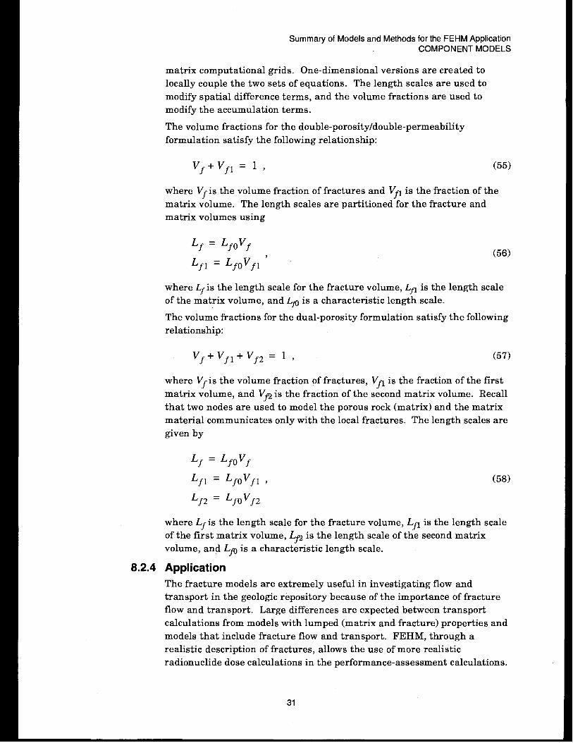
Application
The fracture models are extremely useful in investigating flow and
transport in the geologic repository because of the importance of fracture
flow and transport. Large differences are expected between transport
calculations from models with lumped (matrix and fracture) properties and
models that include fracture flow and transport. FEHM, through a
realistic description of fractures, allows the use of more realistic
radionuclide dose calculations in the performance-assessment calculations.
(58)
31
Summary of Models and Methods for the FEHM ApplicationCOMPONENT MODELS
8.2.5
8.2.6
Numerical method type
Only algebraic manipulations are used in the derivations described in
Section 8.2.6.
Derivation of numerical model
8.2.6.1 Dual porosityComputationally, the volume fractions and length scales are used to create
one-dimensional versions of Eqns. (9), (10), (20), and (76). The length scale
is used to modify spatial difference terms, and the volume factors are used
to modify the accumulation terms (the ~ matrix in Eqns. (25) and (26)).
The geometric factor representing the spatial differencing of the one-
dimensional equation for flow between the fracture and the first matrix
node (analogous to the geometric part of Eqns. (28) and (29)) is given by
VT‘m = I#,f + Lfl) ‘ (59)
where VT is the total volume of the computational cell.
The analogous term for the flow from the first matrix volume to the second
matrix volume is given by
(60)
Using these geometric factors, Eqns. (25), (26), and (27) are modified with
the addition of the following flux terms:
(kpv kPl
Tflf2 ~(pm, v)
–Pf, v) + ~(%, upf,l) ~
(kPvhv—(Pm, v - Pf, v) +‘flfz y, ‘+(%, ~- Pf, J
), and
(kpvhvqv
Tflf2 ~ %, v – Pf, J +)
‘P;;wm, J- Pf, J ,v
(61)
(62)
(63)
where m refers to the matrix and f to the fracture. The equation for the
matrix consists of these transfer terms plus accumulation terms analogous
to those for the fracture and shown in Eqns. (2), (5), (19), and (24). It
should also be noted that the gravity terms are not shown in the transfer
terms above for simplicity but are represented in an analogous way.
The one-dimensional nature of the equations provides a computationally
efficient method for solving the algebraic equations arising from the dual-
32
porosity simulation.
such a simulation:
Summary of Models and Methods for the FEHM ApplicationCOMPONENT MODELS
Equation (64) shows the matrix equation arising from
Ib.
=— bl
bz
(64)
Here, the subscript O refers to the fracture, 1 refers to the first matrix
volume, and 2 refers to the second matrix volume. The x represents the
unknown variable or variable pair. The one-dimensional character of the
matrix diffusion means that the second matrix node can only depend on the
first matrix node. Therefore, the submatrix [Azo] is empty. The fact that
matrix nodes cannot communicate with matrix nodes in other
computational cells means that the submatrices [A21 ] and [A22] are
diagonal, therefore:
{.x2} = [A#[- {bz} - [A211{xI}] , (65)
where the inversion is trivial because [A22] is diagonal. Substituting this
expression into the equation for the first matrix node gives
[AIOI{XO} + [A1l]{x1} +
[44121[A221-1[- {b2} - [A211{xI}I = -{bl} (66)
Rearranging yields
[AIOI{XO} + [[Alll - M12NA221%2111{xI} =
-{ b1}+[A12 [A221-1{b2}
or
{xl} = [&d-t{ ~l}-[Alol{xo}l ,
where
[&] = [Alll - [Z4121[44221%4211
and
{~1} = -{bl} + [A12][A22]-1{b2} .
(67)
(68)
(69)
Summary of Models and Methods for the FEHM ApplicationCOMPONENT MODELS
8.2.7
8.2.8
8.2.9
The inversion and multiplications are trivial because of the diagonal
nature of the matrices involved. Equation (67) may next be substituted
into the equation for the fracture variables. Noting that [Aoz] is empty
(the fracture can only communicate with the first matrix volume) gives
[Aool{xo}+ [Aol][&I]-l[{iI }-[ Alo]{xo}] = -{bo} . (70)
Rearranging terms results in
[[&J-[AoIl[&l-tAloll{xo} = -{ho}+ [Aol][&]-l{ii}. (71)
Equation (71) consists of an augmented fracture matrix of the same form as
the original fracture matrix [Am] . The operations carried out only add a
few percent to the solution time required to solve a single-porosity system.
After the solution of Eqn. (71) is obtained with the methods described in the
GZSOLVE MMS component of Zyvoloski and Robinson (1995), the solution in
the fracture volume can be obtained by using Eqns. (65) and (67).
8.2.6.2 Double-porosity/double-permeability methodThe double-porosity/double-permeability method is analogous to the dual-
porosity method described above with the exception that there is only one
matrix node represented in the double-porosity/double-permeability
method. The matrix node, however, can communicate globally to other
matrix nodes. This approach leads to a system of equations of the form:
(72)
In this set of linear equations, the submatrices Aoo and A 11 are sparse and
Aol and Alo are diagonal. Currently, this system of equations is solved
directly, but research to improve the efficiency of solution is ongoing.
Location
When enabled, the fracture models are called during the equation-
generation and solution phases of the simulation. This point is the same
as that shown for the Flow- and Energy-Transport Equations in Fig. 1.
Numerical stability and accuracy
The same considerations that were discussed in Section 8.1.8 for the Flow-
and Energy-Transport Equations are valid here.
Alternatives
Other approaches to modeling fractures include the equivalent continuum
approach, in which the fracture and matrix properties are averaged, and
the discrete fracture approach, in which the fractures are modeled as
34

Summary of Models and Methods for the FEHM ApplicationCOMPONENT MODELS
8.3
individual computational cells. Both of these methods are included in the
model described in Section 8.1, “Flow and Energy-Transport Equations”.
There has also been some effort to use a combination of numerical and
analytic techniques. In this approach, the matrix flow is represented with
a one-dimensional analytic expression. Because of the nonlinear nature of
the solution, this approach has not been pursued.
Solute Transport ModeIs: Reactive Transport and ParticleTracking
8.3.1
8.3.2
8.3.3
Purpose
The purpose of the reactive-transport and particle-tracking models in the
Solute-Transport Models component is to simulate the movement of tracer
solutes traveling in either the liquid or gas phases. A variety of reactive-
transport capabilities are present in the models. To perform a reactive-
transport simulation, an initial description of each solute concentration in
each phase, transport properties of the fluid and medium, and a
specification of the adsorption model and parameters and any reaction
models are required. The output consists of the final concentration of each
solute in each phase.
Assumptions and limitations
Solutes are assumed to be present in trace quantities such that their
presence does not impact the fluid properties or the computed flow fields.
A related assumption is that chemical reactions do not enter into the
energy balance through endothermic or exothermic reaction terms. If
reactions take place between the fluid and solid phases (dissolution and
precipitation), the transfer of mass is assumed to have no impact on the
hydrologic properties of the medium.
Many other specific assumptions are built into the Solute-Transport
Models component that are related to the nature of the transport and
chemical reaction behavior. These assumptions are treated in
Section 8.3.3.
Derivation
8.3.3.1 Reactive-transport modelThe solute-transport equations in the reactive-transport model
are not directly coupled to the heat- and mass-transfer system
but use the flow rates and temperatures obtained by the heat-
and mass-transfer solution. The mass flux, ~C, source (or sink)
strength, qc, and accumulation term, AC, are defined as followsfor a solute:
7. = cvPvi + clP~~l 7
q. = Cvqv + Ql , and
73)
74)
35
Summary of Models and Methods for the FEHM ApplicationCOMPONENT MODELS
Ac = WV~VP, + CZ~lPl)
The transport equation for a solute is given by
-v“ (cvDmvm’v)- v“ (Cpmlw’l)- v“ (Dcvvcv) - v“ (Dc~vcJ +
(75)
(76)
Here. C is the concentration of the solute. the terma’c,
~ . (llc~ C) is the dispersion term, p,= is an
equilibrium sorption term (see the section below for the
formulation for sorbing solutes), Cr represents the adsorption of
the solute onto the porous media, and in addition, the term qc
includes the source or sink due to chemical reaction. The
chemical-reaction terms are discussed in more detail below in
the section titled “Multiple, interacting solutes.”
Equation (76) is a general equation for a solute present in either the
liquid or gas phases or one that partitions between the liquid and
gas. The model is capable of simulating any of these possibilities, as
well as a solid species, for which only the accumulation and
chemical-reaction terms are present. Several solutes can be
simulated simultaneously and can interact with one another
through the chemical-reaction model. The transport terms can be
set as a function of position, and there is no requirement that they
be the same for all solutes present in a phase.
The next four subsections elaborate on various transport,
sorption, and reaction features of the reactive-transport model.
Dispersion coefficients. The model uses a standard
formulation for the dispersion coefficient, expressed as follows
for the x-direction:
(77)
The Darcy velocity is computed from the solution of the fluid-
flow equation. The dispersivity, ad, and the molecular-
diffusion coefficient, DAB, are properties of the medium, the
fluid (liquid in the above equation), and the solute. Similar
expressions are written for the y- and z-directions.
Adsorbing solutes.
adsorption of species
The general equilibrium model for
onto the reservoir rock is given by Polzer
et al. (1992):
36
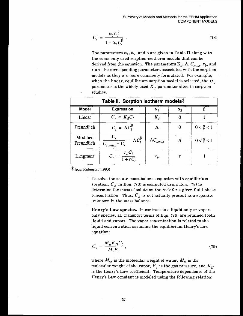
Summaty of Models and Methods for the FEHM ApplicationCOMPONENT MODELS
(78)
The parameters al, Uz, and ~ are given in Table II along with
the commonly used sorption-isotherm models that can be
derived from the equation. The parameters Kd, A, Cmax,rb, and
r are the corresponding parameters associated with the sorption
models as they are more commonly formulated. For example,
when the linear, equilibrium sorption model is selected, the 0! 1
parameter is the widely used Kd parameter cited in sorption -
studies.
Table Il. Sorption isotherm models~
Model Expression al a2 P
Linear c, = Kdcl K~ o 1
Freundlich c, = AC! A o O<pcl
r~ClLangmuir c, = rb
1 + rClr 1
$ from Robinson (1993)
To solve the solute mass-balance equation with equilibrium
sorption, CR in Eqn. (76) is computed using Eqn. (78) to
determine the mass of solute on the rock for a given fluid-phase
concentration. Thus, CR is not actually present as a separate
unknown in the mass balance.
Henry’s Law species. In contrast to a liquid-only or vapor-
only species, all transport terms of Eqn. (76) are retained (both
liquid and vapor). The vapor concentration is related to the
liquid concentration assuming the equilibrium Henry’s Law
equation:
M KHClc,= ;P ,
Vv(79)
where A4W is the molecular weight of water, Mv is the
molecular weight of the vapor, Pv is the gas pressure, and KH
is the Henry’s Law coefficient. Temperature dependence of the
Henry’s Law constant is modeled using the following relation:
37
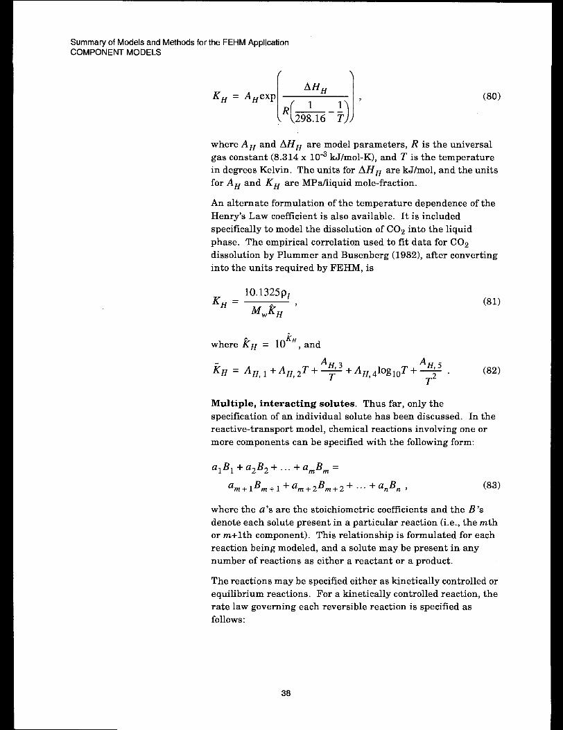
Summary of Models and Methods for the FEHM ApplicationCOMPONENT MODELS
KH = A~exp
[1
H
‘(,::, T)
11’— ——
(80)
where AH and AHH are model parameters, R is the universal
gas constant (8.3 14 x 10-3 kJ/mol-K), and T is the temperature
in degrees Kelvin. The units for AHH are kJ/mol, and the units
for AH and KH are MPa/liquid mole-fraction.
An alternate formulation of the temperature dependence of the
Henry’s Law coefficient is also available. It is included
specifically to model the dissolution of C02 into the liquid
phase. The empirical correlation used to fit data for C02
dissolution by Plummer and Busenberg (1982), after converting
into the units required by FEHM, is
10.1325p1KH =
&?wKH ‘(81)
where KH = 10K~, and
A A H, 5~H = z4H,1+14H,2T+ ~ ‘AH,4@lc)T+ — (82)
T2 “
Multiple, interacting solutes. Thus far, only the
specification of an individual solute has been discussed. In the
reactive-transport model, chemical reactions involving one or
more components can be specified with the following form:
alB1 +a2B2+ . . . +a~B~ =
Bam+l m+l +am~2Bm~2+... +anBn , (83)
where the a‘s are the stoichiometric coefficients and the B‘sdenote each solute present in a particular reaction (i.e., the mth
or m+ lth component ). This relationship is formulated for each
reaction being modeled, and a solute may be present in any
number of reactions as either a reactant or a product.
The reactions may be specified either as kinetically controlled or
equilibrium reactions. For a kinetically controlled reaction, the
rate law governing each reversible reaction is specified as
follows:
38
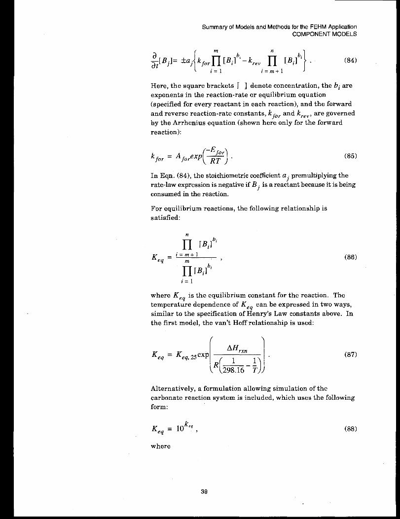
Summary of Models and Methods for the FEHM ApplicationCOMPONENT MODELS
{&?jl= Aaj kforfi U@ - #krev 1fi[B,]” . (84)
,=1 ,Zrn+l
Here, the square brackets [ ] denote concentration, the bi are
exponents in the reaction-rate or equilibrium equation
(specified for every reactant in each reaction), and the forward
and reverse reaction-rate constants, kfor and kreV, are governed
by the Arrhenius equation (shown here only for the forward
reaction):
()‘Efor‘for = Aforexp ~ . (85)
In Eqn. (84), the stoichiometric coefficient a j premultiplying the
rate-law expression is negative if Bj is a reactant because it is being
consumed in the reaction.
For equilibrium reactions, the following relationship is
satisfied:
fi [B,]”~eq=i=m+l
7
fi[B]‘i
i
(86)
i=l
where Keq is the equilibrium constant for the reaction. The
temperature dependence of Keq can be expressed in two ways,
similar to the specification of Henry’s Law constants above. In
the first model, the van’t Hoff relationship is used:
Keq = Keq, 25exp
[1
rxn
‘(,::, T)
11— ——(87)
Alternatively, a formulation allowing simulation of the
carbonate reaction system is included, which uses the following
form:
A
Keq = 10K” ,
where
39
(88)

Summary of Models and Methods for the FEHM ApplicationCOMPONENT MODELS
A AK,q = A,Xn ~+ ArX~,zT+ F+A ,X., ~loglOT + -=@ . (89)
T2
In Eqns. (87) and (89), the temperatures are in degrees Kelvin.
For sorbing species, reaction may occur for solute in the fluid
phase, in the sorbed phase, or both. For the modified
Freundlich isotherm (Eqn. (78)), the total concentration used in
the reaction-rate law for the case of fluid and sorbed-phase
solute participating in the reaction is
[Bj]~O~ = [Bj] + [Bj],OC~ = [Bj] +P,%u$lp
, (90)
PpO(l + a2[Bjlp)
where pr is the bulk-rock density, pp is the fluid density, $ is
porosity, and a 1, a2, and ~ are the sorption isotherm
parameters. Effectively, the second term on the right-hand side
of Eqn. (90) is the equivalent concentration of the sorbed species
if it were present in the fluid phase. The assumption that
reactivity is identical for solute regardless of phase is valid for
radioactive decay but will certainly be incorrect for some
chemical reactions. Thus, FEHM provides an option whereby,
for each species in each reaction, the user may specify whether
the reaction applies to solute in the fluid phase (concentration of
[B~] ), solute in the sorbed phase (concentration given by the
fraction on the right hand side of Eqn. (90)), or both. For two-
phase flow, pP is replaced by ~PPp, where SP is the saturation
of the phase (p) containing the solute.
For reactions involving a solid species, typically a zero-order
chemical reaction is assumed, though this is not required. The
concentration of a solid is expressed in moles of species per kg
rock, whereas all other concentrations in the code are expressed
in moles of species per kg of fluid. The model for solid reactions
undergoing zero-order reactions accounts for the degree of
saturation when computing rates. When there is no solid
present, a solution must be supersaturated (the rate of the
reaction forming the solid must be greater than the rate of the
reaction consuming the solid), or else the reaction is assumed to
not take place.
Finally, when Henry’s Law species are specified as undergoing
chemical reactions, it is assumed that the reaction takes place
for solute in either the liquid or vapor phases but not both. The
user must specify which phase participates in the reaction.
When it is desired that the reaction take place in both phases
40

Summary of Models and Methods for the FEHM ApplicationCOMPONENT MODELS
(say, for a radioactive-decay reaction), the user must specify two
reactions with identical rate expressions, one for the liquid-
borne portion of the solute and one for the vapor-borne portion.
Solute sources and sinks. Solute sources or sinks are
handled in a manner analogous to the fluid-flow sources and
sinks. If there is fluid flow out of the model domain (a fluid
sink), the in-place solute concentration is used in the solute
mass balance. For fluid entering the system, the solute
concentration of the incoming fluid can be specified.
Alternatively, the concentration at a node or nodes can be held
at a fixed concentration. This boundary condition can be either
a source or a sink for solute, depending on the gradient in
concentration at locations adjacent to the node at which the
boundary condition is applied.
8.3.3.2 Particle-tracking modelThe particle-tracking method developed in FEHM views the
fluid-flow computational domain as an interconnected network
of fluid storage volumes. The description that follows is
applicable for steady-state flow fields; the variations in the
method for treating transient flow systems are discussed later.
The two steps in the particle-tracking approach are to
determine 1) the time a particle spends in a given cell and 2)
which cell the particle travels to next. These two steps are
detailed below.
The residence time that a particle spends in a cell is governed
by a transfer function describing the probability of the particle
spending a given length of time in the cell. Thus, this particle-
tracking approach is called the “residence-time transfer
function” (RTTF) method. For a cumulative probability
distribution function of particle residence times, the residence
time of a particle in a cell is computed by generating a random
number between O and 1 and determining the corresponding
residence time. If a large number of particles pass through the
cell, the cumulative residence-time distribution (RTD) of
particles in the cell will be reproduced.
From the solution of the flow field in a numerical model, the
mass of fluid in the computational cell and the mass flow rate to
or from each adjacent cell is obtained. In the simplest case, the
residence time of a particle within each finite-difference cell,
T~ar~, is given by
41
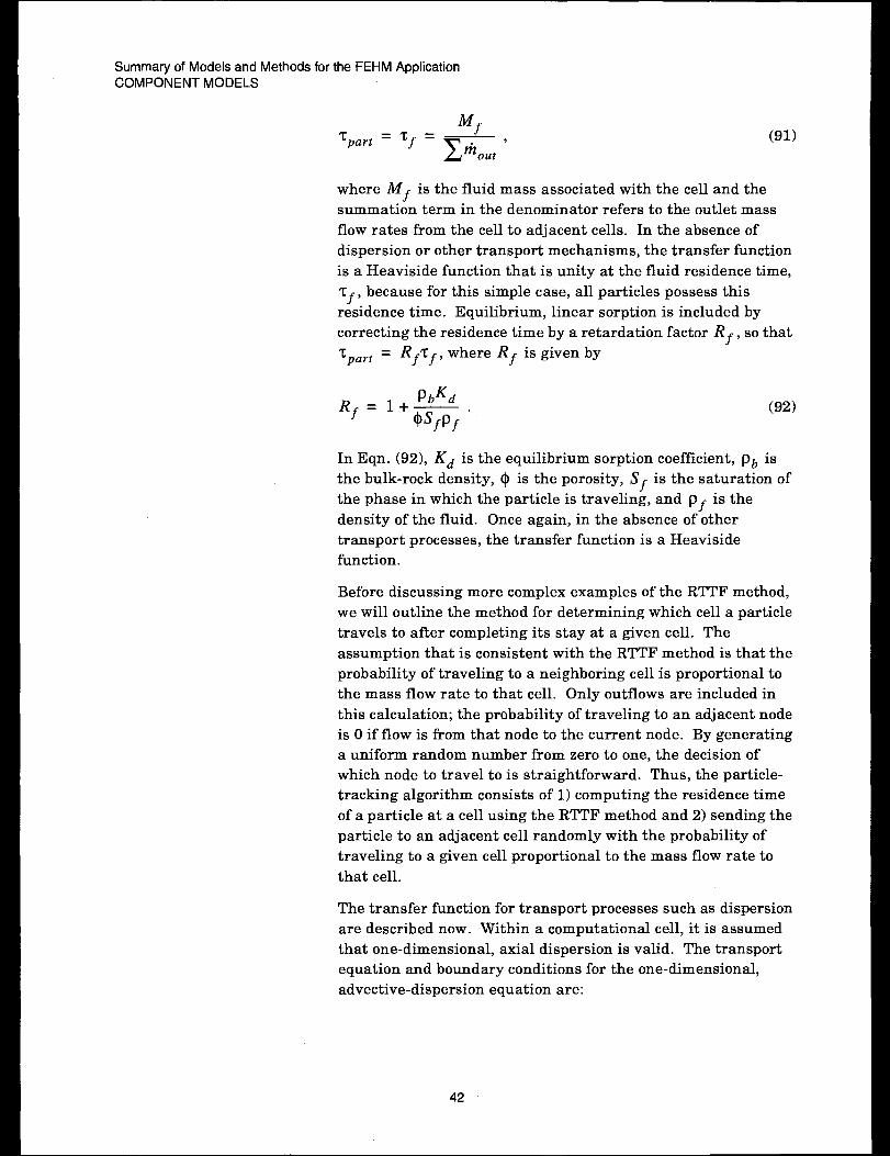
Summary of Models and Methods for the FEHM ApplicationCOMPONENT MODELS
‘f‘part =Tf= ~ ,
x out
(91)
where A4f is the fluid mass associated with the cell and the
summation term in the denominator refers to the outlet mass
flow rates from the cell to adjacent cells. In the absence of
dispersion or other transport mechanisms, the transfer function
is a Heaviside function that is unity at the fluid residence time,
~f, because for this simple case, all particles possess this
residence time. Equilibrium, linear sorption is included by
correcting the residence time by a retardation factor Rf, so that
= Rf~f, where Rf is given by‘part
pbKd‘f = 1 + $Sfpf
(92)
In Eqn. (92), Kd is the equilibrium sorption coefficient, Pb is
the bulk-rock density, $ is the porosity, Sf is the saturation of
the phase in which the particle is traveling, and Pf is the
density of the fluid. Once again, in the absence of other
transport processes, the transfer function is a Heaviside
function.
Before discussing more complex examples of the RTTF method,
we will outline the method for determining which cell a particle
travels to after completing its stay at a given cell. The
assumption that is consistent with the RTTF method is that the
probability of traveling to a neighboring cell is proportional to
the mass flow rate to that cell. Only outflows are included in
this calculation; the probability of traveling to an adjacent node
is O if flow is from that node to the current node. By generating
a uniform random number from zero to one, the decision of
which node to travel to is straightforward. Thus, the particle-
tracking algorithm consists of 1) computing the residence time
of a particle at a cell using the RTTF method and 2) sending the
particle to an adjacent cell randomly with the probability of
traveling to a given cell proportional to the mass flow rate to
that cell.
The transfer function for transport processes such as dispersion
are described now. Within a computational cell, it is assumed
that one-dimensional, axial dispersion is valid. The transport
equation and boundary conditions for the one-dimensional,
advective-dispersion equation are:
42
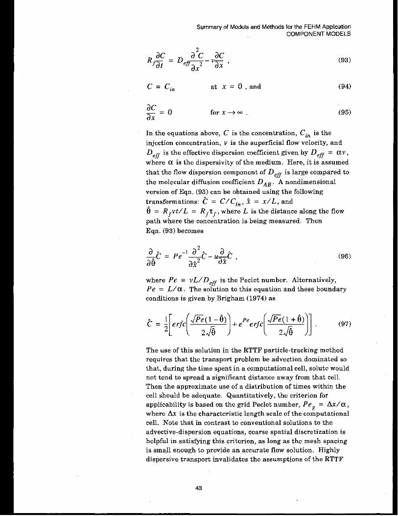
Summary of Models and Methods for the FEHM ApplicationCOMPONENT MODELS
acR~
. ~ a2c W—.‘ffax2‘z ‘
C = Ci~ atx=O, and
~c=oax
(93)
94)
95)
In the equations above, C is the concentration, Cin is the
injection concentration, v is the superficial flow velocity, and
Deff is the effective dispersion coefficient given by ~eff = Uv,
where a is the dispersivity of the medium. Here, it is assumed
that the flow dispersion component of Deff is large compared to
the molecular diffusion coefficient DAB. A nondimensional
version of Eqn. (93) can be obtained using the following
transformations: ~ = C/ Cin, I = x/L, and
6 = Rfvt/L = Rf ~f, where L is the distance along the flow
path where the concentration is being measured. Then
Eqn. (93) becomes
-$t =Pe-1 a2A aA
—c - Uac , (96)a22
where Pe = vL/lleff is the Peclet number. Alternatively,
Pe = L/~. The solution to this equation and these boundary
conditions is given by Brigham (1974) as
The use of this solution in the RTTF particle-tracking method
requires that the transport problem be advection dominated so
that, during the time spent in a computational cell, solute would
not tend to spread a significant distance away from that cell.
Then the approximate use of a distribution of times within the
cell should be adequate. Quantitatively, the criterion for
applicability is based on the grid Peclet number, Peg = Ax/u,
where Ax is the characteristic length scale of the computational
cell. Note that in contrast to conventional solutions to the
advective-dispersion equations, coarse spatial discretization is
helpful in satisfying this criterion, as long as the mesh spacing
is small enough to provide an accurate flow solution. Highly
dispersive transport invalidates the assumptions of the RTTF
43

Summary of Models and Methods for the FEHM ApplicationCOMPONENT MODELS
particle-tracking technique. This is not viewed as a severe
limitation of the method, because accurate solutions to the
advective-dispersion equation are easily obtained by
conventional finite-difference or finite-element techniques for
this case. The niche filled by this new technique is in the
solution of advection-dominated problems involving the
movement of sharp concentration fronts.
For multidimensional flow systems, this method for simulating
dispersion can be extended for the case of dispersion coefficient
values aligned with the coordinate axes. For this case, the flow
direction is determined by the vector drawn from the nodal
position of the cell from which the particle traveled to the current
cell, and the dispersivity for this flow direction is given by
Axctx + AyctY + AZ(XZa=
L(98)
The RTTF particle-tracking technique cannot be formulated
with a longitudinal and transverse dispersion-coefficient model,
because the flow rates between cells are defined rather than the
actual flow velocity at a position. For a dispersion model
aligned to the flow direction, the particle-tracking method, such
as that of Tompson and Gelhar (1990), or a conventional finMe-
element or finite-difference solution to the advective-dispersion
equation should be used.
Matrix diffision. Matrix diffusion has been recognized as an
important transport mechanism for fractured porous media
(Neretnicks 1980; Robinson 1994). For many hydrologic flow
systems, fluid flow is dominated by fractures because of the orders-
of-magnitude larger permeabilities in fractures compared to the
surrounding rock matrix. However, even when the fluid in the
matrix is completely stagnant, solute can move into the matrix via
molecular difision, resulting in a physical retardation of solute
compared to pure fracture transport. This effect has recently been
demonstrated at laboratory scale by Reimus (1995) and at field
scale by Maloszewski and Zuber (1985).
To develop a transfer function for matrix diffusion, an idealized
representation of the transport system must first be generated.
Figure 5 shows the geometry of the model system used for this
purpose. The geometry and flow system consists of equally
spaced, parallel fractures, each of which transmits equal flow.
Fluid in the rock matrix is stagnant. Transport in the fractures
is governed by Eqn. (93) with an additional term qfm on the
right-hand side given by
44

Fracture \
Summary of Models and Methods for the FEHM ApplicationCOMPONENT MODELS
Matrix
+ + + + +Equal flow through each fracture
x
L Y
Figure 5. Model system used to formulate the residence-timetransfer function for matrix diffusion
2%natDABdC(/fm =
bf G ‘Y = b/2
where @real is the matrix porosity and bf is the fracture
aperture. Transport between the fracture and matrix is
governed by the one-dimensional diffusion equation:
2ac
Rf, m% = DAB$ ,
(99)
(loo)
where Rf ~ is the retardation coefficient for the matrix. The
molecular diffusion coefficient is a function of the free diffusion
coefficient of the solute in water and a tortuosity factor to
account for the details of diffusion through the tortuous, fluid-
filled pore network. In this model, DAB is treated as the
fundamental transport parameter, recognizing that it is a
property of both the solute and the medium. Solutions to this
transport problem depend on the nature of the boundary
condition away from the fractures. An analytical solution is
given by Tang et al. (1981) for the semi-infinite boundary
condition ~C’
ay= O as y + co. For the case of plug flow (no
dispersion) in the fractures, Starr et al. (1985) show that the
solution reduces to
45

Summary of Models and Methods for the FEHM ApplicationCOMPONENT MODELS
(101)
The semi-infinite boundary condition between fractures limits
the validity of either of these solutions to situations in which
the characteristic diffusion distance for the transport problem is
small compared to the fracture spacing. However, as long as the
solute has insufficient time to diffuse to the centerline between
fractures, the solutions provided by Tang et al. (1981) or Starr
et al. (1985) are valid to represent the transfer function for the
particle-tracking technique.
Although, in principal, the Tang et al. (1981) solution could be
used for the transfer function, its complex form makes it very
inconvenient for rapidly computing particle residence times.
Instead, a two-step process is used in which the residence time
within the fracture is first computed using the transfer function
for one-dimensional dispersion in Eqn. (97) without sorption.
Then the plug-flow equation with matrix diffusion and sorption
(Eqn. (101)) is used with the value of the fracture residence time
just determined to set the transfer function for the matrix-
diffusion component of the model. To use Eqn. (101) as a
transfer function, a subroutine was developed to determine the
inverse of the error function, that is, the value of Xd for a given
value of yd, such that yd = erf (xd) . The numerical
implementation of this method entails dividing the error
function into piecewise continuous segments from which the
value of xd is determined by interpolation. The use of the two-
step approach is justified because of the principle of
superposition, which allows the decoupling of the dispersive
process in the fracture from the diffusive transport in the
matrix.
Radioactive decay. Radioactive decay is important to many
of the applications for which this model was developed, namely
nuclear waste repository studies. Natural isotopes, such as 36C1and 14C, also require the simulation of radioactive decay. This
phenomenon can be treated by introducing the decay equation
for an irreversible first-order reaction:
(102)
where z age is the particle’s age since entering the system and
k~~ is the rate constant for radioactive decay, which is related
to the radioactive-decay half-life, TI,2, by k~~ = 0.693/T1 ,Z.
46

Summary of Models and Methods for the FEFIM ApplicationCOMPONENT MODELS
In this model, the concept of a fraction of a particle is used to
incorporate radioactive decay into the calculation. The age of a
particle, or time since entering the system, is used in Eqn. (102)
to compute the fraction of the particles remaining at the current
time. When concentration values are computed from the
composite behavior of a large number of particles, this method
accurately accounts for radioactive decay.
Particle sources and sinks. There are two methods for
introducing particles into the flow system: 1) inject the particles
with the source fluid entering the model domain or 2) release the
particles at a particular node or set of nodes. The first method is
used to track injected fluid as it passes through the system. The
number of particles entering with the source fluid at each cell is
proportional to the source flow rate at that node. The method is
the particle-tracking equivalent of a constant solute concentration
in the source fluid. For method 2, an equal number of particles
are released at each node specified regardless of the source flow
rate. In either case, the model calls for the particles to be released
over a specified time interval. The code then computes a starting
time for each particle.
For fluid exiting the model domain, the model treats this flow as
another outlet flow from the node. The decision of whether the
particle leaves the system or travels to an adjacent node is then
made on a probabilistic basis, just as though the fluid sink were
another connected node. When a particle leaves the system, its
sojourn through the model domain is completed; this fact is
recorded as part of the statistics of the simulation.
Transient flow fields. When the RTTF particle-tracking
method is implemented for a time-varying fluid flow system, the
approach is somewhat more complex but still tractable.
Consider a numerical simulation in which a discrete time step M
taken at time t and a new fluid flow field is computed. In this
model, transient flows are handled by treating the new fluid
flow time, tneW, as an intermediate time in the particle-tracking
calculation that the simulation must stop at. The fate of all
particles is tracked from time t to time tneW assuming that the
flow field is constant over this time interval. When the
simulation reaches tmeW,the position of the particle is recorded,
along with the fractional time remaining for the particle at the
cell and the randomly generated y-coordinate of the transfer
function used for that particle in the cell. When the new fluid
flow solution is established, the process continues, but the
remaining residence time for a particle is the time determined
47

Summary of Models and Methods for the FEHM ApplicationCOMPONENT MODELS
from the new transfer function times the fractional time
remaining in the cell.
Another transient effect that must be considered is that the sum
xof the outlet mass flow rates niout in Eqn. (91) does not
necessarily equal the sum of the inlet mass flow rates. When
there is net fluid storage in a cell, the particle-tracking
algorithm uses the sum of the inlet flow rates in Eqn. (91),
whereas Eqn. (91) itself is used when there is net drainage of
fluid.
8.3.4 Applications
For transport calculations using either the reactive-transport or particle-
tracking models, the validity of the solution depends first on the accuracy
of the flow equations. In addition, the reliability of the transport
parameters is also a factor in the representativeness of any transport
simulation.
For the reactive-transport model, the issue of numerical accuracy is
extremely important to the usefulness of the results. The accuracy may be
evaluated by solving the same problem using different size grids and
evaluating the change in the solution. The major source of numerical
errors for transport solutions is anticipated to be the numerical dispersion
resulting from the upwinding of the advection term. Alternative y, the
particle-tracking module can be used for advection-dominated problems to
provide a solution that can be compared to the reactive-transport results.
The primary applications of the particle-tracking model are:
. to generate transport solutions that are able to track sharp fronts in con-
centration without numerical dispersion, thereby allowing results from
the reactive-transport model to be evaluated for numerical accuracy;
● to allow fluid pathways to be mapped out visually using particles that fol-
low the fluid;
c to provide a transport solution for a solute that diffuses into the rock
matrix; and
● to compile statistics on the distribution of fluid ages present at a given
location.
Several limitations of the particle-tracking model should be noted. The
particle-tracking method produces a transport solution that is free of
numerical dispersion when flow is predominantly aligned with the fluid
flow finite-element grid. Grid orientation effects may be present when flow
travels diagonally across the grid. The dispersion model extends the
transport solution beyond a simple “plug flow” transport model, but the
RTTF method is only valid for advection-dominated problems. In regions of
a model domain for which the grid Peclet number is less than about 1, the
method produces inaccurate results. Finally, the matrix-diffusion method
48

Summary of Models and Methods for the FEHM ApplicationCOMPONENT MODELS
is valid only if the solute has insufficient time to diffuse fully between
fractures during the time scale of a simulation.
8.3.5 Numerical method type
For the reactive-transport model, the approximation of the partial
differential equations for solute transport parallels exactly the theory
outlined for the solution of the flow- and energy-transport equations in
Section 8.1.6. The concentrations of all solutes must be solved
simultaneously because the concentrations are coupled through the kinetic
or equilibrium reaction terms. The code employs an option to solve
multiple solute concentration directly using the multiple degree-of-
freedom equation solver for up to four solutes. When more than four
solutes are present, an iterative procedure is required. This method is
outlined in detail in Section 8.3.6.
The RTTF particle-tracking method is a Lagrangian numerical method that
employs transfer functions to compute particle residence times in each cell.
Thus, the time a particle spends in a cell, as well as the decision of which
adjacent cell to travel to next, are determined probabilistically.
8.3.6 Derivation of numerical model
8.3.6.1 Reactive-transport modelBecause many aspects of the reactive-transport numerical
methods parallel the development of the fluid- and energy-
transport numerical method, ordy the parts of the development
that are unique to solute transport are outlined here. Internal
to the code, the chemical reaction terms of the solute mass-
balance equations are always formulated as kinetic expressions
with forward and reverse rate terms. For kinetically controlled
reactions, these rate terms are the two product terms of
Eqn. (84). Equilibrium reactions use the fact that, at
equilibrium, the forward and reverse rates are equal so that
‘eq = ‘for/krev - Forward and reverse rate constants are
forced to be in the correct ratio to simulate equilibrium, and as
long as the rate constants are high enough, equilibrium is
approximated. Of course, it is not known a priori what values to
use for the rate constants. If the values are too low, equilibrium
behavior is not approximated. A less obvious consideration is
that if the values are too high, the rate terms in Eqn. (76)
overwhelm the transport terms in the mass balance and the
reactive-transport problem is not well-posed: the transport part
of the mass balance gets lost in the eolution of the equations.
To circumvent these problems, on the first solute time step, the
model starts at a relatively low value for the forward rate
constant, computes the corresponding reverse rate constant
consistent with the equilibrium constant for the reaction, solves
the reactive-transport problem, then performs a check to ensure
49

Summary of Models and Methods for the FEHM ApplicationCOMPONENT MODELS
that equilibrium is approximated everywhere in the model
domain. The check is
(103)
where ~~ol is a user-defined tolerance parameter defining how
close to equilibrium to force each reaction. Comparing
Eqns. (103) and (86) and making use of the fact that
K = kfO,/k,eV at equilibrium, the value 1 – ~,xn can be seen
ase~he ratio of the equilibrium quotient (the right-hand side of
Eqn. (86)) to the equilibrium constant. Setting y~ol to, say, 0.01
forces this ratio to 0.99, or roughly speaking, 99% of the way to
equilibrium. If the check is not satisfied at all positions, the
minimum value 1 – ~rxn is found, and the forward rate constant
is multiplied by yrXn/kfaCt, where kfaCt is a user-defined
parameter (assumed to be less than 1) that sets the rate at
which the rate constants are increased to approach equilibrium
behavior. Alternatively, kfact can be chosen to be a direct
multiplier to the current forward rate constant, in which case
the value is set greater than 1.
In either case, the process of solving the entire reactive-
transport system is repeated with higher and higher rate
constants until Eqn. (103) is satisfied for all equilibrium
reactions at all positions. In portions of the model domain
where concentrations are low, it is possible that the reaction
rates are low, or even zero, even when equilibrium behavior is
specified. The model can be made to skip the equilibrium check
of Eqn. (103) when the forward rate (the denominator in
Eqn. (103)) is less than a user-specified reaction tolerance
parameter, called rf, ~ol. When a new time step is taken, the
rate constants determined previously are used to restart the
process. These rate constants will usually be sufficient to
assure equilibrium behavior at subsequent time steps, but the
equilibrium check is still performed and rate constants
increased if necessary.
The system of equations representing the mass balance for each
solute results in a coupled system of N~O1x Neq equations. When
kinetics are rapid compared to transport, either because the
rate constants are set large or the equilibrium reaction option is
chosen, the solution technique must be quite robust. The
50

Summary of Models and Methods for the FEHM ApplicationCOMPONENT MODELS
multiple degree-of-freedom solver naturally handles this sort of
strongly coupled system of equations. However, the current
solver handles up to four degrees of freedom (in this case, four
coupled solutes). To solve for more than four solutes, an
iterative procedure has been implemented in which the solutes
are placed into groups of up to four solutes. The code solves the
equations group by group. When a solute is not present in a
group, the current values of concentrations are used in
computing reaction rate terms, but those concentrations are not
unknowns at that particular step of the solution.
Because the calculation of concentrations in groups falling later
in the sequence may impact the mass balance of solutes already
solved for, the entire system is not necessarily converged after
all groups are solved. An outer iterative loop over all groups is
traversed until the residuals of all equations are low. At this
point, the entire system of equations is solved to the specified
tolerance, and a new time step is taken.
8.3.6.2 Particle-tracking modelAll aspects of the numerical model for particle tracking are
discussed in Section 8.3.3.2.
Location
The implementation sequence for either the reactive-transport model or
the particle-tracking model is illustrated in Fig. 1 (page 14). The two
models cannot be run simultaneously in the current version of FEHM.
After a heat- and mass-transfer time step is taken and the flow and
temperature fields are determined, the solute-transport solution is
computed from the previous heat- and mass-transfer time to the current
time. The flow field used for the transport calculations is assumed to be
unchanging during this time.
Numerical stability and accuracy
Reactive-transport model. As in the heat- and mass-transfer solution
discussion (Section 8.1.8), nonlinearities can give rise to problems with the
stability of the solution. The formulation of the problem as a fully coupled,
implicit solution maximizes the likelihood of obtaining a stable, accurate
solution. Accuracy is also intimately tied to the grid discretization, time
step, and dispersion coefficients of the solutes. Advection-dominated
transport with low dispersion coefficients is well known to be difficult to
simulate accurately with finite-difference or finite-element techniques.
Testing the solution against the results of a calculation with smaller grid
spacings and time steps is one way to assess the level of numerical
dispersion. Another way is to compare the solution to a particle-tracking
simulation, which is designed to minimize numerical inaccuracies.
51

Summary of Models and Methods for the FEHM ApplicationCOMPONENT MODELS
Particle-tracking model. The accuracy of an RTTF particle-tracking
solution should be evaluated using the following considerations:
. The dispersion coefficient must be set high enough to avoid grid Peclet
numbers less than 1; in fact, the code sets the Peclet number of a cell to 1
for any value lower than 1.
c Diffusion into the rock matrix must be slow enough that the solute has
insufficient time to diffuse fully to the centerline between fractures.
. If the velocity vectors are not aligned with the fhite-element grid, some
inaccuracies due to grid-orientation effects are to be expected.
● The number of particles in the simulation must be sufficient to minimize
errors induced by statistical fluctuations.
8.3.9 Alternatives
Reactive-transport model. Many different numerical formulations of
the reactive-transport problem are possible. A review of these methods
was performed by Yeh and Tripathi (1989). These models differ in the
number of species that can be simulated and the nature of the chemical
reactions that can be simulated. When equilibrium is assumed for all
reactions, the reaction part of the problem can effectively be decoupled
from the transport and considerable simplification results. For combined
kinetic and equilibrium formulations, Friedly and Rubin (1992) have
shown that similar simplifications are possible. Most models presented in
the literature that use sophisticated chemical submodels are restricted to
simplified flow geometries and flow physics or require a flow solution as
input, and the number of grid points that practically can be simulated is
small.
The reactive-transport model developed here was specifically designed for
use in the context of large-scale two- and three-dimensional simulations. It
was assumed that in the near future, computational resources would be
insufficient to handle a large number of chemical species for a large-scale
problem of many thousands of grid points. Therefore, the model
development assumed that information from other sources (geochemical
codes and literature data for a few key reactions and species) could be
abstracted and distilled into a relatively small number of interacting solutes.
Given this assumption, the logical method of solution was to use the multiple
degree-of-freedom solution technology that is at the center of the FEHM
code. Alternative techniques, such as those referred to above, will be
evaluated and incorporated into future versions of FEHM as needed.
Particle-tracking model. The RTTF particle-tracking modeling
approach in FEHM differs from most groundwater particle-tracking
algorithms reported in the literature (e.g., Tompson and Gelhar (1990); Lu
(1994)). These methods require that the velocity vector be resolved accurately
at each location in the model domain. Doing this usually involves an
interpolation method to obtain the velocity at any position needed based on the
values computed from a flow simulation (at cell faces or nodes, for example).
52

8.4
Summary of Models and Methods for the FEHM ApplicationCOMPONENT MODELS
The algorithm then consists of marching forward in small time steps, computing
the trajectory and a new location of the particle at the new time. Equilibrium,
linear sorption is modeled by introducing a retardation factor to reduce the
particle velocity. Dispersion is handled using a random-walk approach that
displaces the particle a certain amount during each time step so that the
particle samples a different velocity field than it would have in the absence of
dispersion.
By contrast, the approach used in the FEHM particle-tracking algorithm
uses the fluid mass fluxes from node to node as the basis for moving
particles. These are the quantities that are actually known in integrated
finite-difference and finite-element calculations, whereas the velocity
vectors are interpolated results. Thus, the implementation of the RTTF
technique in an existing code like FEHM is straightforward. Another
practical advantage is that the computations are extremely fast:
simulations with several million particles are practical using conventional
workstations. One compromise in the approach is the limitation to
advection-dominated transport systems. This was thought to be a
reasonable compromise, especially in the context of a code that already has
a reactive-transport module that easily handles systems with high
dispersion coefficients.
Constitutive Relationships
8.4.1
8.4.2
8.4.3
Purpose
The densities, viscosities, and enthalpies of water, water vapor, and air are
required for the simulation of flow and energy transport in a porous
medium. These constitutive relations depend on temperature and
pressure. To be computationally efficient, the form of these relations must
be easy to compute and accurate. To satisfy these needs, rational
polynomial fits to the National Bureau of Standards Steam Tables are
used. The models require the pressure and temperature of a node as input,
and they output the densities, viscosities, and enthalpies of the phases.
Assumptions and limitations
At present, several fits of the data are available to the user. These allow
usage of the relations for temperatures up to 360°C and pressures up to
110 MPa. If the variable exceeds the limits of the data, the FEHM code
will restart the time step with a smaller time-step size and try to keep the
variable within the bounds of the data.
Derivation
Pressure- and temperature-dependent fluid properties. A porous
flow simulator, such as FEHM, with heat- and mass-transfer capabilities
requires the functional dependence of the phase densities, the phase
enthalpies, and the phase viscosities on temperature (T) and pressure (P).
Because FEHM is an implicit code that uses a Newton-Raphson iteration,
53

Summary of Models and Methods for the FEHM ApplicationCOMPONENT MODELS
derivatives of the thermodynamic functions with respect to P and T are
also required.
Rational-function approximations are used to estimate the thermodynamic
variables in FEHM, where the rational functions are a ratio of polynomials.
Complete polynomials of order three are used in both the numerator and
denominator. For example, the density is approximated as
Y(P, T)P(p, ‘) = z-p, T) ‘
where
Y(F’, T) = Y.+ YIP+ YZP2 + Y3P3 + Y4T+ Y5T2 +
Y6T3 + Y7PT + Y8P2T + Y9PT2
and
z(P, T) = 20+ ZIP +Z2P2 + Z3P3 + Z4T+ Z5T2 +
Z6T3 -I-Z7PT + Z8P2T + Z9PT2 .
(104)
(105)
(106)
This type of relationship has been shown by Zyvoloski and Dash (1991) to
provide an accurate method for determining parameter values over a wide
range of pressures and temperatures, as well as allowing derivatives with
respect to pressure and temperature to be computed easily.
Polynomial coefficients were obtained by fitting data from the National
Bureau of Standards OSRD database 10, the database used for the NBS/
NRC Steam Tables (Harr et al. 1984). The data fits result in errors less
than one percent and often less than 0.1 percent. The coefficients that are
used in FEHM are valid over the pressure and temperature ranges
0.001< P S 110.0 MPa and 0.001< T < 360°C. Polynomial coefficients for
the enthalpy, density, and viscosity functions are given in Table III in the
Appendix.
Pressure as a function of saturation temperature and temperature
as a function of saturation pressure. The equation for the saturation
line is important for the determination of the phase state of the liquid-
vapor system. The saturation line may be described in a water-only system
as the pressure above which boiling occurs. In a mixture of air or other
noncondensible gas, the saturation line is simply the partial pressure of
water or the vapor pressure of water. Rational-function approximations
are also used for the saturation-line equations:
Y(PV)Y(T) T(pV) = ~ ,
‘“(T) = Z(T) ‘ v
(107)
54
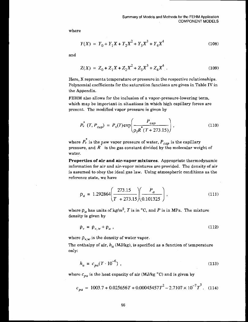
Summary of Models and Methods for the FEHM ApplicationCOMPONENT MODELS
where
Y(x) = Y~+ Y~x + Y2X2 + Y3X3 + Y4X4 (108)
and
z(x) = 20+ 21X+ 22X2 i- 23X3 + 24X4 . (109)
Here, X represents temperature or pressure in the respective relationships.
Polynomial coefficients for the saturation functions are given in Table IV in
the Appendix.
FEHM also allows for the inclusion of a vapor-pressure-lowering term,
which may be important in situations in which high capillary forces are
present. The modified vapor pressure is given by
[
PP: (T, PCaP) = PV(T)exp
cap
1@*(T+ 273.15) ‘(110)
where P; is the pew vapor pressure of water, PCaP is the capillary
pressure, and R is the gas constant divided by the molecular weight of
water.
Properties of air and air-vapor mixtures. Appropriate thermodynamic
information for air and air-vapor mixtures are provided. The density of air
is assumed to obey the ideal gas law. Using atmospheric conditions as the
reference state, we have
pa = 1.292864(T2:::.JI0.122J
(111)
where Pa has units of kg/m 3, T is in ‘C, and P is in MPa. The mixture
density is given by
P, = P,, w+ Pa> (112)
where pV,Wis the density of water vapor.
The enthalpy of air, ha (MJ/kg), is specified as a function of temperature
only:
ha = cp~(T . 10-6) , (113)
where Cpa is the heat capacity of air (MJ/kg ‘C) and is given by
Cpa = 1003.7+ 0.025656T + 0.00045457T2 – 2.7107 X 10⁻⁷T3 . (114)
55
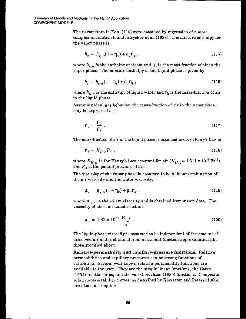
Summary of Models and Methods for the FEHM Application
COMPONENT MODELS
The parameters in Eqn. (114) were obtained by regression of a more
complex correlation found in Sychev et al. (1988). The mixture enthalpy for
the vapor phase is
h, = hv,w(l -q,)+ /zaqv, (115)
where hp ~ is the enthalpy of steam and ~V is the mass-fraction of air in the
vapor phase. The mixture enthalpy of the liquid phase is given by
hl = hz, w(l –qz) +h.~1 > (116)
where hl ~ is the enthalpy of liquid water and ~z is the mass-fraction of air
in the liquid phase.
Assuming ideal gas behavior, the mass-fraction of air in the vapor phase
may be expressed as
~v=kPv “
(117)
The mass-fraction of air in the liquid phase is assumed to obey Henry’s Law or
(118)
where KH, ~ is the Henry’s Law constant for air (KH, ~ = 1.611 x 10⁻⁴ Pa-l)
and Pa is the partial pressure of air.
The viscosity of the vapor phase is assumed to be a Iine.ar combination of
the air viscosity and the water viscosity:
p’. = &Jl -’q,)+ J.Laqv, (119)
where p.v, ~ is the steam viscosity and is obtained from steam data. The
viscosity of air is assumed constant:
~. = 1.82X 10⁻⁸ ‘Q 2“m
(120)
The liquid-phase viscosity is assumed to be independent of the amount of
dissolved air and is obtained from a rational-function approximation like
those specified above.
Relative-permeability and capillary-pressure functions. Relative
permeabilities and capillary pressures can be strong functions of
saturation. Several well-known relative-permeability functions are
available to the user. They are the simple linear functions, the Corey
(1954) relationships, and the van Genuchten (1980) functions. Compositerelative-permeability curves, as described by Klavetter and Peters (1986),
are also a user option.
56
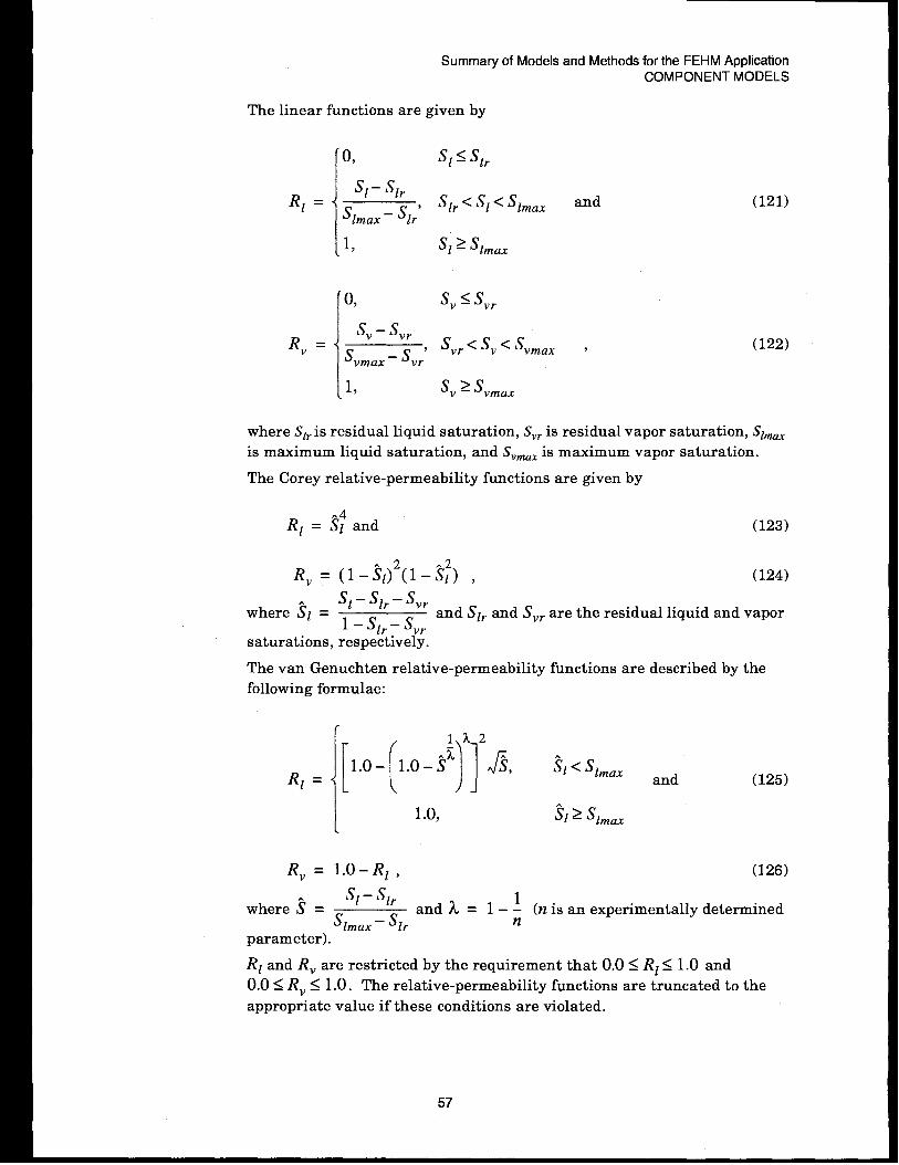
Summary of Models and Methods for the FEHM Amiication
The linear functions are given by
[o,
{
s~- s~rRl = ‘lr < ‘1 < ‘lmaxs lmax - Sir’
[ 1, ‘1> ‘lmax
COMPONENT MODELS
and (121)
10, s,< SV,
1s, - SvrR, =
s - Svr’Svr < s, c Svmax
vmax? (122)
where Szris residual liquid saturation, SV~is residual vapor saturation, Stmax
is maximum liquid saturation, and SVn~Xis maximum vapor saturation.
The Corey relative-permeability functions are given by
I?v = (1-$)2(1-S;) , (124)
A s~– s~r– Svrwhere S1 =
1 – Slr – Svvand Slr and SVr are the residual liquid and vapor
saturations, respectively.
The van Genuchten relative-permeability functions are described by the
following formulae:
1[[ H
la2
1.0– I.o–sz Js, ~1< ‘lma~Rl = and (125)
1.0,
Rv= l. O-R1, (126)
sl – Slrwhere ~ =
s - sirand ~ = 1 – ~ (n is an experimentally determined
lmax nparameter).
R1 and Rv are restricted by the requirement that 0.0 S R1 S 1.0 and0.0< RV S 1.0. The relative-permeability functions are truncated to the
appropriate value if these conditions are violated,
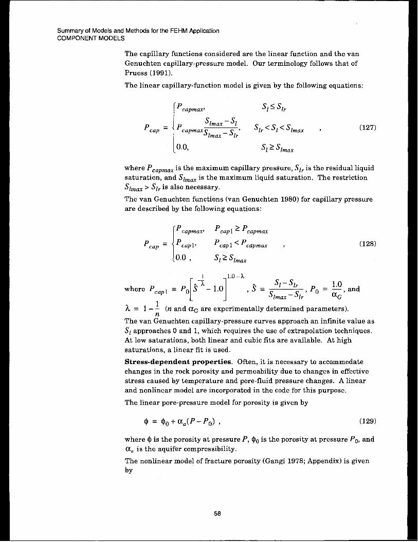
Summary of Models and Methods for the FEHM ApplicationCOMPONENT MODELS
The capillary functions considered are the linear function and the van
Genuchten capillary-pressure model. Our terminology follows that of
Pruess (1991).
The linear ca~
P cap =
Ilary-function model is given by the following equations:
P capmax~ s~5 s~,
s lmax - slP ‘l, <‘1 < ‘lrnax ~capmaxs _s ‘ (127)
lmax lr
I0.0, ‘1> ‘lmax
where PCaPmaXk the maximum capillary pressure, Slr is the residual liquid
saturation, and Slmax is the maximum liquid saturation. The restriction
Slmm > S~r is also necessary.
The van Genuchten functions (van Genuchten 1980) for capillary pressure
are described by the following equations:
P cap =
P capmax~ P Capl> pcapmax
P cap 1~ P capl < ‘capmax , (128)
/0.0, ‘12 ‘lmax
1 l.o–?t
[1
sl- Sl,where Pcap ~ = P. & 1.0 ,s=
s – Sl, ‘P. = ~, and
lmax*
~ = 1 – ~ (n and O!G are experimentally determined parameters).
The van Genuchten capillary-pressure curves approach an infinite value as
S1 approaches O and 1, which requires the use of extrapolation techniques.
At low saturations, both linear and cubic fits are available. At high
saturations, a linear fit is used.
Stress-dependent properties. Often, it is necessary to accommodate
changes in the rock porosity and permeability due to changes in effective
stress caused by temperature and pore-fluid pressure changes. A linear
and nonlinear model are incorporated in the code for this purpose.
The linear pore-pressure model for porosity is given by
where $ is the porosity at pressure
a. is the aquifer compressibility.
(129)
P, $0 is the porosity at pressure PO, and
The nonlinear model of fracture porosity (Gangi 1978; Appendix) is given
by
58
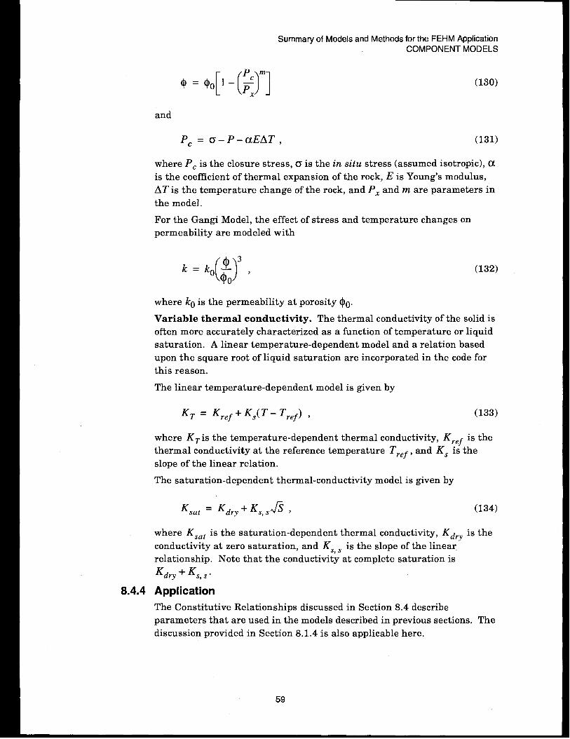
Summary of Models and Methods for the FEHM ApplicationCOMPONENT MODELS
(130)
and
PC = o–P–uEAT, (131)
where PC is the closure stress, G is the in situ stress (assumed isotropic), cx
is the coefficient of thermal expansion of the rock, l? is Young’s modulus,
AT is the temperature change of the rock, and PX and m are parameters in
the model.
For the Gangi Model, the effect of stress and temperature changes on
permeability are modeled with
k .k~’()000 ‘
(132)
where kO is the permeability at porosity @o.
Variable thermal conductivity. The thermal conductivity of the solid is
often more accurately characterized as a function of temperature or liquid
saturation. A linear temperature-dependent model and a relation based
upon the square root of liquid saturation are incorporated in the code for
this reason.
The linear temperature-dependent model is given by
KT = K,,f + KS(T – T,.f) > (133)
where K~ is the temperature-dependent thermal conductivity, KTef is the
thermal conductivity at the reference temperature Tref, and KS is the
slope of the linear relation.
The saturation-dependent thermal-conductivity model is given by
K=sat K~,Y + KS, S$s , (134)
where KSat Ls the saturation-dependent thermal conductivity, KdrY is the
conductivity at zero saturation, and KS ~ is the slope of the linear
relationship. Note that the conductivity at complete saturation is
‘dry + ‘S, S “
8.4.4 Application
The Constitutive Relationships discussed in Section 8.4 describe
parameters that are used in the models described in previous sections. The
discussion provided in Section 8.1.4 is also applicable here.
59

Summary of Models and Methods for the FEHM ApplicationCOMPONENT MODELS
8.4.5
8.4.6
8.4.7
8.4.8
8.4.9
Numerical method type
The Newton-Raphson method is used to calculate saturation and
temperature as a function of pressure. The method has been previously
described in Section 8.1.6.
Derivation of numerical model
The relative-permeability and capillary functions represent the most
nonlinear parts of FEHM, and special consideration has been given to
them. A procedure similar to that used by Nitao (1988) is used to restrict
the van Genuchten capillary function, Eqn. (128), to finite values when
approaching zero saturation. The procedure is simple. At a low saturation,
usually input by the user, the van Genuchten functions are replaced with
linear fits that match the van Genuchten function at the specified
saturation value and attain a maximum value, usually twice the value at
the specified saturation, at zero saturation. This new capillary pressure is
then used in the calculation of the relative permeability. The formulation
in FEHM differs from Nitao’s implementation in that it uses a cubic spline
fit to match both the value and the slope at the specified saturation. At
zero saturation, the coefficients of the spline are adjusted so that a zero
slope and a zero second derivative are achieved. This approach assures a
monatomically increasing function for the capillary pressure.
Location
The Constitutive Relationships are used to obtain the parameters that
define the Flow- and Energy-Transport Equations. Referring to Fig. 1
(page 14), the box labeled “Get thermodynamic parameters” represents
calls to routines that form the Constitutive Relationships.
Numerical stability and accuracy
The formulation of the Constitutive Relationships is directly related to the
overall accuracy of the FEHM application. The accurate formulation of the
water properties described in Section 8.4.3 was motivated by the need to
have accuracy combined with computability. The discussion in
Section 8.4.6 showed the need to have continuous and finite values of the
constitutive functions. The authors believe there is still much work to be
done in the area of extending the range of the functions as well as finding
representations that will allow better convergence of the Newton-Raphson
iteration.
Alternatives
FEHM uses analytic derivatives of the constitutive functions described in
Section 8.4. The TOUGH code described by Pruess (1991) and the variant
of TOUGH used by Nitao (1988) use numerical differences of the fluid- and
energy-balance equations in the Newton-Raphson iteration. Both of the
methods have merit. The numerical-derivative approach allows for
possibly faster incorporation of new fluid physics models, whereas the
60
Summary of Models and Methods for the FEHMApplicationEXPERIENCE
analytic-derivative approach uses fewer iterations on tested problems
(Reeves 1993).
The functional representation of the constitutive models could be replaced
by a tabular formulation. Several available codes have used tabular input
for capillary and relative-permeability data.
tabular representations in future versions.
9.0 EXPERIENCE
The FEHM computer code and its predecessors have been
I?EHM will also incorporate
used on a wide variety of
problems ranging from geothermal to environmental remediation and radioactive
transport. When used in conjunction with its available grid-generation package and
postprocessing tools, it has been a successful tool for modeling very complex geological
settings and coupled-fluid processes. When benchmarked against other codes, it has
been shown to be extremely competitive (Reeves 1993).
61

I
0)rcl
[1
Table Ill. Polynomial coefficients for enthalpy, density and viscosity functions
knth alpy I.)enslty VlscosltyLiquid Vapor Liquid Vapor Liquid Vapor
Y~ 0.25623465e-03 0.31290881e+O0 O.10000OOOe+Ol 0.1 5089524e-05 0.174091 49e-02 -O.13920783e-03
Y] 0.1 0184405e-02 -O.10000OOOe+Ol 0.1 7472599e-01 O.10000OOOe+Ol O.18894882e-04 0.98434337e-028~ Y2 0.22554970e-04 0.25748596e-01 -0.20443098e-04 -O.l OOOOOOOe+Ol -0.66439332e-07 -0.51504232e-03
E Yj 0.34836663e-07 0.38846142e-03 -0.17442012e-06 -0.1 6676705e-02 -0.23122388e-09 0.62554603e-04
2 Y~ 0.41769866e-02 0.1 1319298e-01 0.49564109e-02 0.401 11210e-07 -0.31534914e-05 0.27105772e-04%m Yj -0.21244879e-04 0.20966376e-04 -0.40757664e-04 0.25625316e-10 0.1 1120716e-07 0.84981906e-05EaJ.- Y~ 0.25493516e-07 0.74228083e-08 0.50676664e-07 -0.40479650e-12 -0.48576020e-10 0.34539757e-07
g Y~ 0.89557885e-04 0.19206133e-02 0.50330978e-04 0.43379623e-01 0.28006861e-07 -0.25524682e-03
6 Yg 0.10855046e-06 -0.10372453e-03 0.33914814e-06 0.24991800e-02 0.23225035e-09 0.0000OOOOe+OO
Yg -0.21720560e-06 0.59104245e-07 -0.18383009e-06 -0.94755043e-04 0.47180171e-10 0.12316788e-05
Z* O.1000OOOOe+Ol 0.1251131 9e+O0 0.10009476e-02 0.12636224e+O0 O.1000OOOOe+Ol O.1000OOOOe+Ol
kz~ 0.23513278e-01 -0.3606131 7e+O0 0.16812589e-04 -0.30463489e+O0 0.10523153e-01 O.1000OOOOe+Ol
%c Z2 0.48716386e-04 0.58668929e-02 -0.24582622e-07 0.27981880e-02 -0.22658391e-05 -0.1000OOOOe+Ol.-E0 Zj -0.19935046e-08 0.99059715e-04 -0.17014984e-09 0.51132337e-05 -0,31796607e-06 -0.1000OOOOe+Olct% z~ -0.50770309e-02 0.44331611e-02 0.48841156e-05 0.59318010e-02 0.29869141e-01 O.1000OOOOe+Ol
z Zja 0.57780287e-05 0.50902084e-05 -0.32967985e-07 0,80972509e-05 0.21844248e-03 O.1000OOOOe+Ol
E z~ 0.90972916e-09 -0.10812602e-08 0.28619380e-10 -0.43798358e-07 -0.87658855e-06 -0.22934622e-03.-.-: ‘7
-0.58981537e-04 0.90918809e-03 0.53249055e-07 0.53046787e-03 0.41690362e-03 O.1000OOOOe+Ol
8 z~ -0.12990752e-07 -0.26960555e-04 0.30456698e-09 -0.84916607e-05 -0.25147022e-05 0.0000OOOOe+OO
Zg 0.45872518e-08 -0.36454880e-06 -0.12221899e-09 0.48444919e-06 0.22144660e-05 0.25834551e-01
Pressure range O.001-llOMPa 0.001 -20MPa O.001-llOMPa 0.001 -20MPa O.001-llOMPa 0.001 -20MPa
remperaturerange 15-360”C 15-360”C 15-360°C 15-360°C 15-360”C 15-360°C
d
0
0
g
-umz0x
I
I
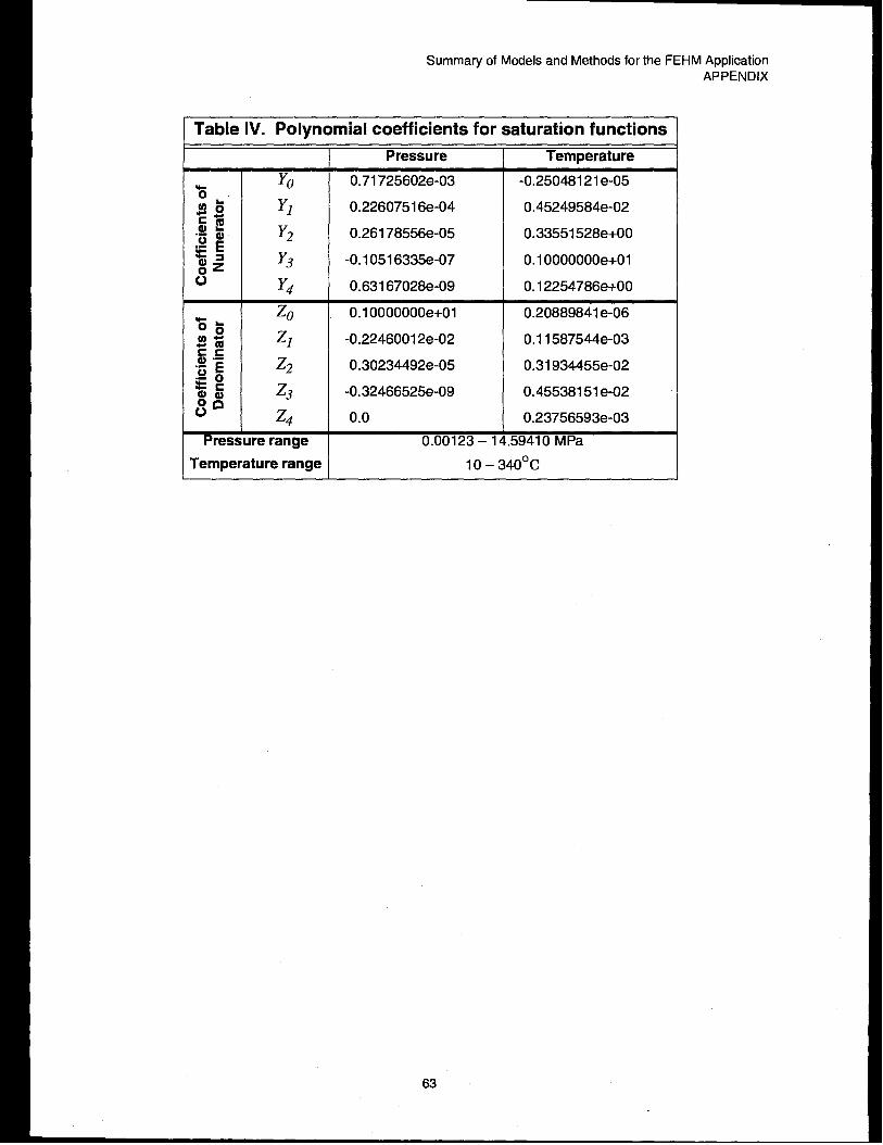
Summary of Models and Methods for the FEHM ApplicationAPPENDIX
Table IV. Polynomial coefficients for saturation functions
Pressure range
Temperature range
! Pressure
0.71 725602e-03
0.22607516e-04
0.261 78556e-05
-0.1051 6335e-07
0.631 67028e-09
O.10000OOOe+Ol
-0.2246001 2e-02
0.30234492e-05
-0.32466525e-09
0.0
0.00123-1
Temperature
-0.25048121 e-05
0.45249584e-02
0.33551 528e+O0
O.1000OOOOe+Ol
O.12254786w-00
0.20889841 e-06
0.1 1587544e-03
0.31 934455e-02
0.45538151 e-02
0.23756593e-03
59410 MPa
10 – 340”C
63
Recommended