Pontificia Universidad Catolica de Chile
Facultad de Fısica
Loop Quantum Gravity
and
Effective Matter Theories
by
Marat Reyes
Thesis submitted for the Ph.D. degree in physics
at the Faculty of Physics, Pontificia Universidad Catolica de Chile.
supervisor : Dr. Jorge Alfaro
Commission : Dr. Marcelo Loewe
Dr. Jorge Gamboa
Dr. Maximo Banados
December, 2004
Santiago – Chile

Contents
Acknowledgements ii
Summary iv
1 Introduction 1
1.1 Quantum gravity: Origins and motivations . . . . . . . . . . . . . . . 1
1.2 Status and overview: free quantum field theories . . . . . . . . . . . . 4
1.2.1 Fock quantization: particle interpretation . . . . . . . . . . . . 5
1.2.2 Functional quantization: field interpretation . . . . . . . . . . 6
1.3 First historical attempts . . . . . . . . . . . . . . . . . . . . . . . . . 8
1.3.1 Gravity is non-renormalizable . . . . . . . . . . . . . . . . . . 8
1.4 Main inputs: Concepts and tools in loop quantum gravity . . . . . . 9
1.4.1 Diffeomorphism concept in Einstein’s theory . . . . . . . . . . 11
1.4.2 Dirac quantization . . . . . . . . . . . . . . . . . . . . . . . . 12
2 The loop quantum gravity formalism 14
2.1 Hamiltonian Formulation . . . . . . . . . . . . . . . . . . . . . . . . . 15
2.2 Geometrodynamics quantization . . . . . . . . . . . . . . . . . . . . . 18
2.3 New canonical framework . . . . . . . . . . . . . . . . . . . . . . . . 20
2.3.1 First order variables . . . . . . . . . . . . . . . . . . . . . . . 20
2.3.2 The Palatini action and self-dual action . . . . . . . . . . . . . 21
2.4 Loop quantization . . . . . . . . . . . . . . . . . . . . . . . . . . . . 22
2.4.1 Holonomies . . . . . . . . . . . . . . . . . . . . . . . . . . . . 23
2.4.2 Spin Networks . . . . . . . . . . . . . . . . . . . . . . . . . . . 24
2.4.3 Area Operator . . . . . . . . . . . . . . . . . . . . . . . . . . . 25
i
2.4.4 Volume Operator . . . . . . . . . . . . . . . . . . . . . . . . . 26
3 Yang Mills effective model 27
3.1 Electric sector . . . . . . . . . . . . . . . . . . . . . . . . . . . . . . . 28
3.2 Magnetic sector . . . . . . . . . . . . . . . . . . . . . . . . . . . . . . 32
3.3 The total regularized Hamiltonian . . . . . . . . . . . . . . . . . . . . 33
3.4 Holonomies expansion . . . . . . . . . . . . . . . . . . . . . . . . . . 34
3.4.1 The Abelian case . . . . . . . . . . . . . . . . . . . . . . . . . 35
3.4.2 The non-Abelian case . . . . . . . . . . . . . . . . . . . . . . . 37
3.5 Electric flux expansion . . . . . . . . . . . . . . . . . . . . . . . . . . 40
3.6 Semiclassical analysis: A general scheme . . . . . . . . . . . . . . . . 42
3.7 Yang Mills effective Hamiltonian . . . . . . . . . . . . . . . . . . . . . 45
4 Higgs effective model 52
4.1 Higgs regularization . . . . . . . . . . . . . . . . . . . . . . . . . . . . 53
4.2 Momentum and field covariant expansions . . . . . . . . . . . . . . . 59
4.3 The Higgs effective Hamiltonian . . . . . . . . . . . . . . . . . . . . . 60
4.3.1 Kinetic part . . . . . . . . . . . . . . . . . . . . . . . . . . . . 61
4.3.2 Derivative part . . . . . . . . . . . . . . . . . . . . . . . . . . 63
4.3.3 Higgs effective Hamiltonian . . . . . . . . . . . . . . . . . . . 65
5 Conclusions and Perspectives 66
A Non-abelian electric flux integrals 67
B Higgs: kinetic contribution 69
C Higgs: derivative contribution 72
ii

Acknowledgements
I want to thank...
•
•
•
•
•
•
•
•
iii
Summary
Since Loop Quantum Gravity (LQG) i.e., an approach to quantize gravity, was first
formulated in the pioneering work of T. Jacobson and L. Smolin, it has undergone
a rapid increase of original ideas leading to profound insights and unexpected con-
nections between: gravity, loops, knots and gauge theory. After two decades of
active research in the field, the LQG approach is by now considered viable as well
as a promising candidate to quantize General Relativity. The approach is a minimal
attempt to combine the ideas of Quantum Mechanics and General Relativity. Mini-
mal in the sense that it sticks with the standard formulation of Quantum Mechanics
and General Relativity, but implementing rigourously the diffeomorphism symme-
try of General Relativity. The notion of diffeomorphism symmetry by its own leads
to a fully background independent and non-perturbative formulation of Quantum
Gravity. Partial culmination of these ideas had become crystalized in states of the
gravitational field i.e., possible occurrence of 3-geometries with discrete eigenvalues
and purely constructed from combinatorial principles.
The impetus in the LQG approach is mainly attributed to the success casting
a consistent and formal Kinematical theory that solves the problems of quantum
gravity in a great extent. Progress has been made by matching the black hole con-
straint, and by the recent inspired phenomenological models that put close possible
scenarios to test loop quantum gravity effects. These effects have an opportunity
to be probed in cosmological events and in particle physics beyond the Standard
Model.
Moreover, the Hamiltonian of the Standard Model coupled to gravity, supports
a representation based on densely defined operators. The resulting Hamiltonian is
anomaly free and completely finite without renormalization. From these Hamilto-
iv
nians we obtain the effective Hamiltonians that contains quantum gravity effects.
More precisely, in this thesis we focus in two objectives, first we present the
departing theory from which we obtain the effective models, the Loop Quantum
Gravity formalism. Secondly, we derive the Yang Mills and Higgs effective models
that contains quantum gravity corrections.
In the introduction we summarize the arguments that supports the idea that
a quantum theory of spacetime is important. Certainly, these arguments are not
in the category to be considered formal proofs, instead they try to motivate the
construction of this theory. The claim that a fundamental theory should not have
place for infinities, resume them.
We review in chapter 2 the Hamiltonian formulation of General Relativity and
the LQG formalism in which we pay special attention to the subset of kinematical
constraints, this roughly includes the spin networks basis and geometric operators
spectra.
Last chapters are central part of our investigation, they include a detailed anal-
ysis of the method we have developed to obtain Yang Mills and Higgs effective the-
ories. Both effective theories were obtained using semiclassical states picked around
a flat three metric and defined to preserve rotational invariance. We compute ex-
pectation values of Hamiltonians which describe particle propagation and predict
near Planck energy scales the breakdown of Lorentz invariance.
v
Chapter 1
Introduction
1.1 Quantum gravity: Origins and motivations
Quantum Gravity is an attempt to amalgamate in a single consistent theory, two of
the major revolutionary ideas of contemporary physics, Quantum Mechanics (QM)
and General Relativity (GR). The research in this direction has been intense over
the past seventy years, attracting a lot of ingenious ideas and the investments of
tremendous efforts. However, until date all the proposed models to accomplish
this synthesis have shown to be incomplete or inconsistent. The final program
of quantizing GR has become extremely elusive and out of our immediate reach;
reports and current status can be found in [2, 3]. Nevertheless, one has to recognize
that enormous progress has been made in several directions, the most important
approaches are among Superstring [10, 11], Non-commutative Geometry [12] and
Loop Quantum Gravity (LQG), (for an introduction of LQG, see [4, 5], for the first
use of loop variables see [1], and for textbooks see [6, 7] and more recently [8, 9])
which we honestly remark is not minor considering the complexity of the task.
The two theories proposed to unite are GR and QM, both are consistent but
also disconnected descriptions of the world, each one separately, provide robust
contributions to our knowledge. Let us briefly comment and highlight on their basic
aspects.
The framework introduced by Einstein’s theory harmoniously allows to accom-
modate spacetime and matter in a geometrical language. The concepts taking part
1
in the foundational physics of Newton like action-at-distance and absolute observer
had been replaced with new notions. In modern terminology, gravitational field is
identified with spacetime geometry and absolute observer with general covariance.
This is perhaps amongst the most radical changes taking place in physics.
Einstein equation Rµν− 12gµνR = 8πGTµν is a non linear, second order differential
equation for the metric tensor, which synthesize and codes the dynamics of the
theory. A large variety of geometric entities in the manifold, such as line elements,
Riemann curvature and geodesics are specified through the metric. In that way, a
broad range of gravitational phenomena are related to the interplay of matter and
geometry, yielding, planetary orbits, gravitational lensing, black holes, etc.
Gravitational interaction is well known to persists over cosmological scales and
neglected in high energy phenomena. Therefore, the scenario of gravity becoming
crucial for local high energies processes, as suggested by quantum gravity, is quite
astonishing. Then, the statement that gravity deals exclusively with the very large
seems to be premature yet.
On the other side of our knowledge, the agenda to quantize all the forces has
seen to be gloriously achieved in all known matter field theories, culminating in the
celebrated SU(3)× SU(2)× U(1) Standard Model (SM). Standard Model is a the-
ory of strong and electroweak interactions. It accommodates gluons, W and photons
acting as force carriers between quarks and between leptons. All fundamental inter-
actions are described within the SM formalism, except gravity. The data obtained in
accelerator experiments, with relativistic particles colliding at energies of the order
of 102 Gev, are extremely precise and in high accordance with theoretical predic-
tions, also of course the experiments in condensed matter physics, quantum optics
etc, which are ruled with the non relativistic Schrodinger equation. At date, no
fundamental interactions of physics deviates from this universally quantum-matter
implementation.
However and in spite of the successful implementation of Quantum Mechanics
in the matter sector, a deep understanding of the steps that defines the theory is
still missing. These fundamental issues, when treating with the gravitational system
might turn to be important and not more allowed to be ignored.
Nowadays, it is widely known that the standard methods of functional quanti-
zation are sterile when applied to GR; this is the first explanation why gravity has
2
not been quantized yet. Its origin lies on the fact that divergent diagrams occur-
ring in the perturbative serie can not be removed by a renormalization procedure.
A natural questions then arises: Are the basic assumptions in GR or QM fully
correct?. Several and different approaches, work on the idea that a quantum de-
scription of spacetime requires a modification of the two basic theories GR and QM,
some more drastic than others (see [13, 14, 15, 16, 17, 18]). Nevertheless, if one
insist to apply a perturbative approach in gravity by replacing GR at high energies,
just like Fermi theory was replaced by electroweak theory, then the main objec-
tion is that metric splitting and background dependence, implicit in perturbation
theory, means to lose active diffeomorphism invariance of GR. Another reaction to
the non-renormalizability of gravity is support the thesis that quantum corrections
have negligible effects on the gravitational interaction which is extremely weak and
therefore argue that the unification of GR and QM might be useless, at least from an
empirical point of view. We are aware that this is a possibility, but contradicts the
next point [ 2 ], and presents a departure from the historical evolution characterized
in physics toward a reductionist viewpoint of Nature.
The present status of experiments gives no strong clue, although, some argu-
ments sheds some light on why is important to search for this quantum gravity
theory. The most popular claims are related to the role of observables and to the
unavoidable inconsistencies resulting from the formulation of semiclassical quantum
gravity:
[ 1 ]. A fundamental theory must have finite observables and consequently mean-
ingful predictions. To solve the problem of having divergent observables in a theory
the theoretical framework must be extended by replacing some of the basic assump-
tion. An old hope in physics is the idea that quantum gravity could provide the
extended framework to remedy the following singularities.
(a) Cosmological objects such as black holes are characterized to have infinite
curvature in the origin, R(0) → ∞, high matter density regions reflect themselves
in that way.
(b) The problem of initial condition has not been solved in cosmological models.
A description of the origin of the universe might come from the elucidation of some
3
aspects that quantum gravity theory must confront.
(c) Standard Model is saturated with two kind of singularities. One shows up
at fixed order when arbitrary high momenta are summed over in the perturbative
expansion. The second kind of divergency, worst in nature, comes from the whole
series expansion. This last one is not cured even using a renormalization procedure
as in the first case. The argument here is that quantum gravity could provide a
natural gravitational regulator for these infinities, preventing integrals from ultravi-
olet divergencies. Mainly due to space discreetness which is expected to arise from
the quantum gravity theory, therefore prohibiting arbitrary short distance and high
momenta availability.
[ 2 ]. A classical gravitational field interacting with a quantum system lead to
inconsistencies. The key line of argument is roughly, after assuming Gµν = 〈ψ |Tµν | ψ〉, solutions for the metric needs to specify if there has been wavefunction
collapse after any measurement on the system. This fact leads to violation of either,
uncertainty principle, momentum conservation, signals faster than light, or other
unwanted results. [19]
1.2 Status and overview: free quantum field the-
ories
In the next subsections, we want to give a brief overview of the axiomatic involved
in the quantization of free field theories. The main motivation here, is to point out
some misleading generalizations in the methods used in free quantum field theories
when they are applied to the gravitational system. We will show two possible in-
terpretations given to free Quantum Field Theories (QFT), the particle and field
interpretations. The first interpretation is strongly motivated by the action of the
Poincare group while the second resembles more the general procedures of Quan-
tum Mechanics. Canonical methods to quantize gravity uses the latter which is best
4
suited to give physical meaning to the gravitational field and because the gauge
symmetry underlying GR is the diffeomorphism group and not the Lorentz group.
GR is a constrained system, thus the tools employed in canonical quantization of
gravity are in many aspects different of those handled in traditional QFT. Here we
will show those first differences.
1.2.1 Fock quantization: particle interpretation
Quantizing a system with infinite degrees of freedom, is commonly known as second
quantization. In particle physics this is normally realized with the use of creation
and annihilation operators that allows to build up the quantum field with all its
basic harmonic excitations. And permits to connect by acting on the vacuum, the
distinct particle Hilbert subspaces of finite harmonic oscillators. Fock space then is
defined by the direct product of these individual Hilbert spaces.
The axiomatization of free QFT are usually given in terms of Wightman axioms
[23, 24], which we proceed to summarize
1. Unitary Representation.
The existence of a unitary and continuous representation of the Poincare group
P realized in Hilbert space H: P → U(a, Λ), a and Λ being typical displacements
and rotations in spacetime.
2. Spectral Condition
We require for the momentum operator P µPµ ≤ m2; P 0 ≥ 0
3. Unique Vacuum
The trivial representation U(a, Λ) = 1 correspond to a state which is invariant
under all Poincare transformations called the vacuum Ω0
U(a, Λ) Ω0 = Ω0
4. Covariance
5
Consider the smeared field operator φ(f) =∫
d4x φ(x)f(x). The set of linear
combinations of the form φ(f1)...φ(fn)Ω0 lie dense in H, hence the vacuum is said
to be cyclic. The field satisfy the covariant property
U(p)φ(f)U(p)−1 = φ(f · p) p ∈ P
5. Microscopic Causality
Let the supports of ~f and ~g be spacelike separated then the operators φ(~f) and
φ(~g) must satisfy the relation [φ(~f), φ(~g)] = 0.
Recall that in free field quantization, for instance in the case of a scalar field, the
bilinear operator Nk = a†kak which is called number operator, have integers eigenval-
ues and is a constant of motion. Quantum states which are classified according that
integer are mapped by a†k and ak into states with increased or decreased that inte-
ger. The operators a†k and ak are interpreted as creating and annihilating quanta.
Therefore, the notion of quanta being a observer independent quantity, heavily relies
on the property of transformation of the operators among themselves. They must
transform covariantly under the action of Poincare group, as can be seen in the ex-
pression for the bilinear operator. In that way, the notion of particle in conventional
QFT does not depend on the inertial system.
In resume, Fock space is essentially motivated because carries a unitary rep-
resentation of the Poincare group, which as we have said, permits to consider an
n-particle state observer-independent, and therefore quanta as a absolute notion.
The absence of this group in the GR case, is another good reason to consider a
different approach than the particle interpretation.
1.2.2 Functional quantization: field interpretation
We start with the basic variables, the configuration variables φ(x, t) and its conju-
gate momenta π(x, t). Both fields, are defined to satisfy the following equal time
commutation relation
6
[φ(x), π(y)
]= i~δ(3)(x− y) (1.1)
Next we choose a representation of the equal time commutations relations, for
which we define, respectively, smeared coordinates and momenta Q, P of the fields
φ and π in terms of the following basis e1, ..., ek, ν = 1, ..., k, for example at time
t = 0, by
Qn(e, 0) =
∫φα(x, 0)eν(x)d3x (1.2)
Pn(e, 0) =
∫πα(x, 0)eν(x)d3x, n ∈ (α, ν) (1.3)
which could generate temporal evolution through a Hamiltonian H, accordingly
to
Pn(x, t) = ei~Ht Pn(x, 0) e
−i~ Ht (1.4)
Qn(x, t) = ei~Ht Qn(x, 0) e
−i~ Ht (1.5)
A representation of (1.1) is obtained by choosing state vectors as functionals of the
classical configuration space Q and belonging to the Hilbert space L2(Q, dµ(Q)),
where dµ(Q) is the measure.
Qn(x)Ψ[φ(X)
]= Qn(x)Ψ
[φ(X)
](1.6)
Pn(y)Ψ[Q(X)
]= −i~
δΨ[Q(X)
]
δQn(y)(1.7)
The Schrodinger equation is
H(Q,−i~δ
δQ)Ψ
[Q(X); t
]= i~
∂Ψ[Q(X); t
]
∂t(1.8)
After a measurement is made of the classical field configuration, the quantity
PB =
∫
B
|Ψ[Q(X); t
]|2dµ(Q) (1.9)
is the probability that the result lie in the set B.
7
1.3 First historical attempts
The quantization program in high energy physics, applies only for free fields prop-
agating in a fixed and flat background, as we have seen in the Wightman axiomati-
zation. Therefore, approximative methods as perturbation theory and quantization
on curved backgrounds have been developed to treat with interacting fields, which
indeed are the ones we experience in real life. The perturbative method in SM relies
on the availability to define a unitary operator that describes time evolution and
connects free asymptotic quantum states in the far past and future. Haags theorem
demonstrates that the interaction picture does not really exists, at least you can
write down a perturbative serie that approximates it, but then you need to renor-
malize the theory. What is called renormalization is the mechanism by which order
by order the serie can be made artificially finite, this is surmounted by redefinition
of certain parameters in the Lagrangian as masses, charges and fields. This scheme
has succeeded in the SM, although the convergence of the whole serie is totally lost
and left without control.
The perturbative approach in GR fails because the gravitational field is not
renormalizable as we will see in the next subsection. This is one of the reasons why
the non-renormalizability of gravity could be considered disappointed. But let us
emphasize that even in the case that perturbation techniques were viable in GR we
would have to deal in consequence with the same open problem that characterize
the SM, the convergence of the whole series.
Let us briefly sketch what happens when trying to implement the perturbative
expansion in the gravitational system.
1.3.1 Gravity is non-renormalizable
A naive check to know if a theory is renormalizable is by power counting. Consider
the dimensionless action S in the units ~ = c = 1. The theory for a certain in-
teraction g∫ Lint is renormalizable if the superficial degree of divergence 4 is not
negative, where the mass dimensionality of the coupling constant is g = M−4. The
8
reason is that for momenta K ≤ M lower than the mass scale of the coupling pa-
rameter g = M−4 the interaction is suppressed by the term ( kM
)4 ≤ 1 and therefore
we lose predictability, for else we need a mass scale higher than the accessible ener-
gies of the system. The mass dimensionality depends on the superficially degree of
divergence 4 = 4 − d −∑f nf (sf + 1), where nf is the number of fields of type f
and sf , is 0 , 1/2 , 1 , 0 for scalars and graviton, fermions, massive vector field, and
photons respectively.
The first check for gravity, is whether the superficial degree of divergence satisfies
the above condition. For which we refer the readers to the calculation developed in
[20] using the background field method. To sketch the calculation let us consider
the perturbative treatment of the Einstein Hilbert action∫
d4x√
gR with the usual
split of the metric around a fixed background plus the perturbation, in most cases
the background is chosen to be the Minkowskian flat metric, in the following way,
gµν(X) = ηµν +√
Ghµν(X) (1.10)
At first order we obtain an interaction term
√Gh(∂h)(∂h) + ... (1.11)
Making the power counting we see that 4 = 4 − 2 − 3 = −1, and GR is not
renormalizable neither including supersymmetry.
1.4 Main inputs: Concepts and tools in loop quan-
tum gravity
At this point, the first attempt to quantize gravity have failed, when looking for
other approaches as the canonical ones, we will have to consider a set of constraint
and deal with their solutions (treated in detail in the next chapter). This can be
done in two different ways, the first one is solving the constraints at the classical level
9
and then quantizing (phase space reduced methods), and the second is quantizing
and then trying to solve the constraints. The latter, which will be revised in the
sequel, is named Dirac quantization, and is the one used in the LQG approach.
On the other hand, fair to say, solutions to the Hamiltonian constraint better
known as Wheeler DeWitt equation, have never been found in the metric approach
(geometrodynamics approach) not even a consistent regularization. Things improve
in the LQG approach, following the Dirac quantization program and using Ashtekar
variables, some naive solutions can in fact be given, but a complete understanding
of the theory, which amounts to solve the Hamiltonian constraint remains an open
problem.
Due to the many obstacles when trying to quantize gravity, the discussion to a
great extent has been centered on the requirements asked to the quantum gravity
theory. Therefore, in the formulation of Quantum Gravity theory one must decide
among all the basic structures one wants to preserve. The loop approach tries to
implement the quantization program without changing the traditional structures of
both QM and GR, and holding further the diffeomorphism symmetry of GR.
The additional requirement of having active diffeomorphism invariance in the
theory, might seen at first not enough to produce a substantial change. However, as
we would see, a relevant shift in the mathematics involved would take place, with
states of the gravitational field, spin network relying ultimately in combinatorial
terms, and amazing implications which by now belong to the principal ingredients
of the LQG approach, as discreteness of 3-geometries. The notion of space that we
have gained in our everyday experience, continuum and smooth has to be considered
only an approximation accounting for many basic excitations that are discrete in
nature and that should become evident, as we descend to the fundamental levels of
space.
Progress has been achieved from the LQG perspective in understanding the non-
renormalizability of gravity. Essentially because the separation of the gravitational
field into a classical background plus a quantum correction neglects non-perturbative
effects, such as discreteness of 3-geometries that contradicts the assumption of hav-
ing availability of arbitrary short distances.
As we have already mentioned, the irreconcilability of quantum theory and gen-
eral relativity, is by now, one of the important problems left unsolved in theoretical
10
physics. The problems, had lead us to deal with the interplay of concepts taking
part in the final theory. The common sensation, however, and definitely the biggest
obstacle that undermines the final program of quantum gravity, which should be
always kept in mind, is the shortage confronting experimental data which permits
to test the different models and the existent theories in dispute.
1.4.1 Diffeomorphism concept in Einstein’s theory
The goal in this subsection is review the key notions firmly established by now in
the GR formalism, as well as their lesser known implications. More precisely, we
want here to emphasize the role of diffeomorphism symmetry and show how this
induces the concept of relationalism in physics.
The GR legacy has brought a substantial upgrade in the understanding of Nature.
Firstly due to the identification of gravitational field with spacetime geometry. This
has changed the old vision that all the things evolve on top of a fixed absolute
background structure, the same one that Newton needed to formulate his theory.
The rigid background is today considered as a dynamical entity governed through
the Einstein’s equations. Secondly, the underlying gauge invariance of GR, general
covariance or active diffeomorphism invariance implies a spectacular renaissance of
the idea of relationism in physics. The notion of relationism has returned with
tangible physical meaning and not only as a product of philosophical thoughts. Let
us explain this concept in more detail.
The GR formalism is invariant under the group of diffeomorphism Diff(M).
They are transformations defined over the manifold M, mapping the spacetime
points to the same manifold while the relevant physical quantities are left invariant.
This signifies that all the possible locality information regarding individual points in
the manifold gets virtually removed by the symmetry, not even to transfer points to
a set of equivalent regions, more instead to only one big equivalent region, the whole
manifold. This is achieved by means of all the C∞ transformations. Holding further
this idea, it can be realized that space and time must lack of absolute meaning i.e.,
points can not be referred to some-where or some-when, for else the implicit fact that
GR has to be described in a fully relational form [21, 22]. In this sense, relational
11
means that what is capable to give a precise description to things are only through
relationships, very different of what happens in Newtonian theory where a system
defined by a flat non-dynamical background is such that all the physical effects of
other system ultimately relies on this absolute one.
Furthermore the quantum implementation of this symmetry is well captured in
the picture of spacetime arising in LQG, in which space is defined by the manner
loops are knotted to each other on a single point and subject to change in time. The
rationale in GR is different from other physical theories formulated on dependent
backgrounds, as the entire SM in which the view is that fields evolve on top of
a background. It is meaningful in QED theory to consider a par creation and
ask for the direction of the emitted particles, because the direction is supposed
to be referred to an external absolute structure. Spacetime objects in GR rests
only through relationships, any background structure breaks this symmetry albeit
in many cases the theory may still be able to be formulated in a passive invariant
fashion.
Diffeomorphism is capable to indicate us the presence of a background, this
extra information involves the dynamics of the theory itself. Passive transformations
depends on how the theory are mathematically formulated.
1.4.2 Dirac quantization
In this subsection we will review the Dirac algorithm for constrained systems which
is the one used in the LQG approach. A more detailed discussion can be found in
[25].
Consider a classical system with Hamiltonian H(qi, pi), with qi a set of canonical
variables with canonical momenta pi. Whenever a system with non independent
variables is formulated, a set of constraints is obtained and defined by the relations
φa(qi, pi) = 0 i = 1, 2, ...a (1.12)
First class constraints are defined to satisfy,
12
φa, φb = Cdabφd (1.13)
Second class constraints do not satisfy this relation. Although, there are methods
to bring second class constraints into first class constraints. After some manipulation
involving the lagrange multipliers λa, the time evolution of a function O(q, p) satisfies
O(q, p) = O, H+ λaO, φa (1.14)
O is defined to be an observable if O, φa = 0. first class constraints generate
gauge transformations connecting physical trajectories in a restricted phase space
constraint surface. The Hamiltonian can be written H ′ = H + λaφa.
Now, let us resume the steps leading to the Dirac quantization of systems with
constraints
1. Define an auxiliary Hilbert space H(aux) and pick a polarization such that
quantum states are functionals of the configurations variables Ψ[Q]
2. Find a representation for the classical algebra into commutators
[P (x), Q(y)] = −iδ(3)(x− y) (1.15)
with self-adjoint operators on a Hilbert space of states
Q = Q (1.16)
P = −iδ
δQ(1.17)
3. Symmetries are represented as constraints, then one has to impose quantum
constraints annihilating physical states, narrowing the H(aux) to a physical Hilbert
space H(phy)
4. We need now a inner product in the physical Hilbert space in order to compute
expectation values and make physical predictions
5. Construct a set of observables that could be interpreted
More references for this subsection are found in [26, 27, 28, 29, 30]
13
Chapter 2
The loop quantum gravity
formalism
Now that we have discussed the concepts involved in the loop approach, let us turn
to the review of the mathematical formulation.
The Hamiltonian formulation of GR was developed in the sixties by Arnowitt,
Deser and Misner (ADM) [31]. In rigor the formalism constitutes the starting point
of canonical approaches. To describe dynamical evolution, the Hamiltonian is re-
quired to depend on a time parameter. Therefore, spacetime manifold M of 4-
dimensions will be arbitrary spilt in 3-dimensional space plus time direction which
is unphysical. The explicit covariance of the theory will be spoil, although the
constraints will tell us that the theory is invariant under any such choice of coordi-
natization. Thus, all the concepts analyzed in the previous sections are going to be
canalized through the constraints.
The use of complex phase space for GR (Ashtekar or self-dual variables) remark-
ably leads to a simplification of the algebraic structure of the constraint. Allowing
for the first time to found an overcomplete basis of solutions for the Hamiltonian
constraint. These solutions called Wilson loops provides the name ”loop” and hints
on the advantages of a formulation of GR in terms of Ashtekar variables [32].
14
2.1 Hamiltonian Formulation
Consider a global hyperbolic 4-manifold M with topology R× S, and S a compact
3-manifold representing space and t ∈ R unphysical time. Next, cover M with a
foliation into Cauchy surfaces Σt and define t as a global time function and tµ a
time-like vector representing the flow of time, both obeying tµ∇µt = 1.
Let us write an imbedded space metric qµν as
qµν = gµν + nµnν , (2.1)
with nµ a normal vector to Σt and with nµnµ = −1. The vector field tµ can be
decomposed in its normal nµ and tangential Nµ components to the surface Σt in the
form,
tµ = Nnµ + Nµ. (2.2)
N receives the name of lapse function, as it measures the change in proper time
while Nµ is called shift vector relating normal displacements. Written in a particular
system of local coordinates (x, t) and in terms of the quantities (qµν , N,N i), the line
element ds reads,
ds2 = −N2dt2 + qab(dxa + Nadt)(dxb + N bdt). (2.3)
Note that the metric qµν acts as projector on Σt, therefore verifying qµν nν = 0
and qµν qνρ = qρµ, therefore in what follows qµν will be considered a space metric
written with space indices only.
An important object that describes the velocity of qab as it moves normally to
the surface Σt, is given by the extrinsic curvature Kµν :
Kµν = q σµ ∇σnν , (2.4)
or the alternative definition given by,
15
Kµν =1
2L~nqµν , (2.5)
where L is the Lie derivative along the vector ~n. With the same considerations
as before we will write the extrinsic curvature with spatial indices.
The tensors qab and Kab are called first and second fundamental forms in Σt
respectively, they behave as Cauchy data for the metric, just like the potential
vector Aa and the electric field Ea are Cauchy data for the electromagnetic tensor
Fµν . Phase space consist in the 3-metric qab and in the extrinsic curvature Kab.
They allows to cast the system in canonical form.
After some manipulation the Einstein-Hilbert action S =∫
d4xR written in the
variables q and K reduces to
S =
∫dtd3xN
√q((3)R + KabK
ab −K2), (2.6)
with q the 3-determinant of qab, where√
g = N√
q, and using the following
notation K = Kaa .
The action is now conveniently expressed in terms of variables that are space
functions and which evolves in time, so let us follow the traditional steps in the
canonical quantization program. With this purpose, we choose the 3-metric qab
to play the role of position, while its associated conjugate momenta results to be,
πab = ∂L∂qab
=√
q(Kab − K2qab). Then, after working out the Hamiltonian density
and using the Legendre transform of the Lagriangian density L, we finally arrive to
the expression
H(q, π) =
∫
Σ
d3xH =
∫
Σ
d3x√
q(NC + NaCa) (2.7)
where we have defined
C = −(3)R + q−1(πabπab − 1
2π2) (2.8)
and
16
Ca = −2∇b(q−1/2πab), (2.9)
the notation is such that ∇a, is the torsion-free covariant derivative compatible
with qab and π2 = (πaa)
2.
The fact that the Hamiltonian contains no time derivatives with respect to the
lapse and the shifts functions, means that N and Na are Lagrange multipliers,
instead than true dynamical variables. It can be shown that,
C = 0 and Ca = 0. (2.10)
The above equations are instantaneous laws satisfied on shell i.e., on each hy-
persurface Σ, analogous to the Gauss constraint in electromagnetism. In electro-
magnetism the Gauss law constraint, tell us how to control the redundant degree
of freedom of the gauge theory U(1), by pointing out, that not any electric field re-
sults to be a proper solution. In here we have the same situation, with only certain
allowed regions in phase space.
The constraints C and Ca are called Hamiltonian and spatial diffeomorphism
respectively, because when we set ~N to zero, the Hamiltonian of GR turns out to
be, see eq (2.7),
C(N) =
∫
Σ
NCq1/2d3x. (2.11)
Considering the phase space function J , it can be shown that C(N) generates
infinitesimal gauge transformations
δNJ = C(N), J. (2.12)
Thus, the Hamiltonian constraint C(N) generates diffeomorphisms in a normal
direction that corresponds to the direction of the flow of time. Now, if we set the
lapse N to zero,
17
~C( ~N) =
∫
Σ
NaCaq1/2d3x (2.13)
and we arrive to,
δ ~NJ = ~C( ~N), J. (2.14)
As before, we see that C( ~N) generates diffeomorphism in the ~N direction with
displacements tangent to Σt.
The Hamiltonian and diffeomorphism constraint can be shown to verify the Pois-
son algebra,
~C( ~N), ~C( ~M) = ~C(L ~M~N) (2.15)
~C( ~N), C(M) = C(L ~N~M) (2.16)
C(N), C(M) = ~C( ~K) (2.17)
where K is defined to be Ka = qqab(N∂bM −M∂bN).
2.2 Geometrodynamics quantization
Until this point, GR has been canonically formulated and the gauge character of
gravity directly related to the constraints, that in turn play the role of spacetime
diffeomorphism generators. The Hamiltonian of GR has seen to vanish on shell,
since it’s a linear combinations of vanishing constraints. At this stage we could
think that the dynamics of the theory is dominated by a trivial Hamiltonian, which
is not the case. More precisely, is an indication that the GR Hamiltonian is not a
true Hamiltonian, instead generates spacetime diffeomorphisms and therefore tell us
that space and time can not be defined as something absolute.
18
Our next step is to apply the rules of quantization to the gravitational system
we have derived, picking for example a polarization for the state vectors in terms
of metric variables Ψ(q). Thereafter, we seek for a representation of the symplectic
algebra expressed in terms of metric variables, which lead us to the next step in
the Dirac quantization program for constrained systems. Promote constraints to
operators while requiring physical state vectors to lie in the kernel of the constraints,
Cµ(q, π)Ψ(q) = 0. (2.18)
However and unfortunately, the Cµ functions involve terms in which the canoni-
cal variables appear non polynomially multiplied, not even analytically on the metric
qab, so we must confront operator ordering problems; different orders of writing down
equivalent classical formulas for the constraints yield different operators in the quan-
tum level. One can, at least in principle, seek for regularized expressions for the
constraints, where operators are to be defined in terms of limits of smeared field
variables. Up to date no one has yet demonstrated a consistent choice of canonical
variables and operator orderings in which the constraints equations behave in the
above sense. This technical issue is the constraints implementation problem
and is where the program first stalls. Let us go further and analyze the dynamic of
the theory. We have said that the Hamiltonian density vanishes on physical states
by virtue of equation (2.7) and (2.10). The dynamics of the theory, then, is not
dominated by the Hamiltonian, rather describes the states that are invariant under
all spacetime diffeomorphism. This is the time problem in quantum gravity; this
feature is related to the meaning of time as something determined intrinsically by
the theory (in terms of geometry), rather than by an external structure. In order
to compute expectation values and relevant quantities involved in any measurable
phenomena we will require a physical inner product and a real Hilbert space. We
must factor out somehow the gauge group of Diff(Σ) when one performs an in-
ner product. This resembles the factorization done in the functional integral, and is
called the inner product problem. These three problems are the major roadblock
we face when we try to quantize gravity by means of canonical technics (for a more
detailed discussion on these points see [7, 37]).
19
2.3 New canonical framework
Now that we have summarized the main list of problems encountered in the program
of geometrodynamics quantization, let us change to a different approach that will
lead us close to the basic of the LQG formalism. We will give a chance to the
so called first order formulation, which introduce tetrads and spin connections
as new variables in phase space. These new variables introduce extra degrees of
freedom in the theory, providing an additional solution to the Einstein equation
together with a new subset of constraints related to rotational invariance in tangent
space. The new variables allow to describe the system more like a Yang Mills (YM)
theory. We will exploit this fact using all the machinery developed to quantize these
gauge systems. However constraints will retain their non polynomial character with
no substantial progress when we try to implement the quantum version of constraints
and with all the subsequent attached problems we have describe before.
Nevertheless, if in addition phase space of GR is extended using self dual variables
or the so called Ashtekar variables [32], that is, a complex phase space with self
dual connections and tetrads, then the constraints notably simplifies. Wilson loops
solutions of the Hamiltonian and Gauss constraint, are in here, the first sign of the
loop notion arising.
2.3.1 First order variables
The key point of the next step is to shift the description of the system, basically from
metric variables to connection ones. First let us define tetrads and spin connections.
A set of basis vectors eIa are called tetrads or vielbeins if the metric of space
time looks locally flat, ie.
gµν = eIµe
Jν ηIJ I, µ = 0, 1, 2, 3 (2.19)
We can perform a a Lorentz transformation on the flat indices I at every point
in spacetime, they are called local Lorentz transformations, or perform usual
20
general coordinate transformations or diffeomorphisms on curved indices
µ. Comparison of the covariant derivative on two different bases permit us to write
the following relationship between spin connection w Iµ J and ordinary connection Γν
µλ
w Iµ J = eI
νeλJΓν
µλ − eλJ∂µe
Iλ (2.20)
We can think on eIµ and w a
µ b as a vector and tensor valued one form respectively
[36].
2.3.2 The Palatini action and self-dual action
With the same assumptions regarding the manifold structure of the previous section,
the Palatini action is defined by a curvature 2-form ΩIJµν = ∂[µω
IJν] + [ωµ, ων ]
IJ the
connection 1-form ωIJµ and the tetrad eµ
I as,
S(e, w) =
∫d4x e ea
IebJΩIJ
ab , (2.21)
where e =√−g is the determinant of the tetrad.
After performing the usual spacetime decomposition, we arrive to an additional
solution, which is eaI = 0 and to a new constraint, the Gauss constraint DaeI
a = 0
[37].
The main idea of the modern formulation is to introduce Ashtekar variables [32]
or the self-dual Lorentz connection +A keeping the tetradic construction. This
extra structure requires complex phase space variables, therefore requires to extend
the differential geometric structure of traditional GR to complex GR. Under ap-
propriate reality conditions we can recover the standard theory which makes them
totally equivalent. The spacetime decomposition of this new action introduce a fun-
damental change in the kind of constraints; this in part relies on the fact that the
new connection entails information of both variables qab and Kab, like Bargmann
or holomorphic variables in the solution of the quantum harmonic oscillator. We
define a Lorentz connection by AIJa = −AJI
a and the internal Hodge dual of a
21
Lorentz connection mapping element of the space of connections to itself defined by∗T IJ = 1
2εIJ
KLTKL; any Lorentz connection can be write by a sum of self-dual and
anti-self dual parts A = +A + −A with ∗A = ±i ±A. In terms of self and anti self
dual parts ±A = (A∓ i ∗A)/2. The other basic field besides the self-dual connection
is the tetrad eIµ, the proposed self dual action is,
S(e, +A) =
∫
M
d4x e eµI e
νJ
+F IJµν . (2.22)
It can be shown that the curvature of a self dual Lorentz connection is self dual
∗F = iF Where we have defined the internal Hodge dual of the curvature F as
(∗F )IJµν = 1
2εIJ
KLFKLµν . Now we proceed with the usual decomposition of spacetime;
gauge fixing the internal vector nI = edInd = (1, 0, 0, 0) allow to consider only 0I
components of internal indices.
The Hamiltonian becomes,
H =
∫
Σ
1
2N ~Fab( ~Ea × ~Ea) + Na ~Fab · ~Eb + Λ ·Da
~Ea (2.23)
With EaI =
√qea
I and the self dual connection Aia. They satisfy the Poisson
bracket relation
Aia(x), Eb
j (y) = iδbaδ
ijδ
(3)(x− y) (2.24)
with new constraints,
Gi = DaEai Ca = Eb
i Fiab H = εij
k Eai Eb
jFkab (2.25)
and obeying a different constraint algebra [5].
2.4 Loop quantization
The use of Ashtekar variables has led to a simplification in the constraints. To
proceed we must choose a representation of the relation (2.24) and pick a polarization
of the functionals in terms of connection variables for instance, such as
22
AiaΨ(A) = Ai
aΨ(A) (2.26)
Eai Ψ(A) =
δ
δAia
Ψ(A) (2.27)
and then promote the constraints to operators equations. First we will consider
a order for the constraints, with the triads to the right (2.25),
Gi = Daδ
δAia
Ca = F iab
δ
δAia
H = εijkF iab
δ
δAja
δ
δAkb
(2.28)
Gauss constraint require that states be gauge invariant functionals states of
the connection A, therefore states can be described by the loop states Ψγ(A) =∏i Tr(h(A, γi)) as the basis states for quantum gravity. They allow us to control the
diffeomorphism constraint and are solutions of the Hamiltonian constraint. However
one of the difficulties of these objects is that they form a overcomplete basis.
It can be shown that the Gauss and the Diffeomorphism constraint generates
gauge transformations and diffeomorphisms on the wavefunctionals Ψ(A). A first
inspection suggest to consider Wilson loops W (A) = Tr(Pexp
∮Aadxa
)which are
well known to be gauge invariant functionals under transformations of the connec-
tion A, and therefore automatically solutions of the Gauss constraints. We would
continue to require these states to be annihilated by the Diffeomorphism constraints
and then continue with the Hamiltonian constraints, with the hope to finish at the
end with a genuine Hilbert space, with physical states belonging to it.
2.4.1 Holonomies
Let a curve γ be defined as a continuous, piecewise smooth map from the interval
[0, 1] into the 3-manifold M ,
γ : [0, 1] −→ M (2.29)
s 7−→ γa(s) , a = 1, 2, 3 . (2.30)
23
The holonomy or parallel propagator h[A, γ], of the connection A along the curve γ
is defined by
h[A, γ](s) ∈ SU(2) , (2.31)
h[A, γ](0) = 11 , (2.32)
d
dsh[A, γ](s) + Aa
(γ(s)
)γa(s) U [A, γ](s) = 0 , (2.33)
where γ(s) := dγ(s)ds
is the tangent to the curve. The formal solution of (2.33) is
given in terms of the series expansion
P exp
∫ 1
0
dsA(γ(s)
)
=∞∑
n=0
∫ 1
0
ds1
∫ s1
0
ds2 · · ·∫ sn−1
0
dsn A(γ(sn)
) · · ·A(γ(s1)
). (2.34)
h[A, γ](s) = P exp
∫
γ
ds γa Aia
(γ(s)
)τi ≡ P exp
∫
γ
A , (2.35)
for any matrix-valued function A(γ(s)
)which is defined along γ.
Here P denotes path ordering, i.e. the parameters si are ordered with respect to
their moduli from the left to the right, or more explicitely s1 ≤ s2 ≤ . . . .
2.4.2 Spin Networks
A graph Γn = γ1, . . . , γn is a finite collection of n piecewise smooth curves or edges
γi, i = 1, . . . , n, respectively, embedded in the 3-manifold M , that meet only at their
endpoints.
A spin network is a generalization of a graph, namely a colored graph. More
precisely, by definition a spin network is a triple s = (Γ,~j, ~N), where to each link
γi we assign a non-trivial irreducible representation of SU(2) which is labelled by
the numbers ~j = ji. Let Hj1 , . . . ,Hjkbe the Hilbert spaces of the representations
associated to the k links. Consider a node p where the k links meet, and associate
to it the Hilbert space Hp = Hj1
⊗....
⊗Hjk. Fix an orthonormal basis element
24
Np in Hp. An element Np of the basis is called a coloring of the node p. A spin
network state can be defined by taking holonomies at each link associated to the j
representation and contracting it with the elements of the basis in Hp where links
meet. The spin networks states Ψ(A) can be shown to satisfy the orthonormal
condition
< ΨS | ΨS′ >= δΓ,Γ′δj,j′δS,S′ (2.36)
2.4.3 Area Operator
The spectrum computation of geometric operators in the loop representation were
done taking advantage of their non locality properties [78]. Using the complete
basis of spin network states is possible to calculate operators spectrums that are
observables in the Dirac sense.
A surface Σ is a 2-dimensional submanifold embedded in M . The associated
embedding is given by the map X : Σ → M and is characterized by local coordinates
xa, a = 1, 2, 3 on M and coordinates on the surface σµ = (σ1, σ2), µ, ν = 1, 2.
Σ : (σ1, σ2) 7→ xa(σ1, σ2) (2.37)
The pullback metric gΣ and the normal na on Σ are given by
gΣµν =
∂xa
∂σµ
∂xb
∂σνgab and na =
1
2εµνεabc
∂xb(~σ)
∂σµ
∂xc(~σ)
∂σν(2.38)
The area is then
A[Σ] =
∫
Σ
d2σ√
detgΣ =
∫
Σ
d2x
√1
2!εµ1µ2εν1ν2gΣ
µ1ν1gΣ
µ2ν2
=
∫
Σ
d2x√
nanbEaiEbi (2.39)
25
After regularizing the area A(Σ) the area operator A(Σ) is given by
A(Σ) = limε→∞
∑
n(ε)
√Ei(Σn)Ei(Σn) (2.40)
where we have define the smeared operator
Ei(Σ) = −i~G∫
Σ
d2σna(~σ)δ
δAia(x(~σ))
(2.41)
Finally, the eigenvalues corresponding to the area operator are given by the
expression
A(Σ) = 8πβ~G∑
l
√jl(jl + 1) . (2.42)
Where jl labels de SU(2) representation associated to the link l crossing the
surface Σ .
2.4.4 Volume Operator
Let us consider the volume of a three dimensional region R, this is given by
∫
R
d3x√
detg (2.43)
g is the three-dimensional space metric. In the same way as in the case of the
area operator, a regularization for the volume operator is needed.
We will not show the technical steps in the derivation of the volume operator
but merely give its final expression, which is
V =1
4l3p
∑i
√aibici + aibi + bici (2.44)
where p , q and r are the colors of the three adjacent link of the node i. And where
we have defined
p = ai + bi q = bi + ci r = ci + ai (2.45)
26
Chapter 3
Yang Mills effective model
Let us go now on to the construction of the Yang Mills effective theory when diffeo-
morphism invariance, geometric operators, spin networks, and what we have study
in the previous chapters are extended or included to matter dynamics. The concrete
implementation given in here is due to the calculations of our work which forms part
of the results of this thesis.
First attempts to include matter in the framework of loop quantum gravity,
were done in the pioneering work [48, 49]. For an approach based on the Kinemat-
ical framework for diffeomorphism invariant theories of connections, see [50]. The
posterior breakthrough came by generalizing to diffeomorphism invariant quantum
field theories, including, besides connections, also fermions and Higgs fields. And
facing directly the task of including matter fields in the Kinematical scheme with
well defined adjoint relations and using the volume operator to solve order ambi-
guities and finiteness of the theory [51]. In that way a consistent representation
with holonomies-like excitations of quantum fields, was successfully implemented to
describe all the sectors of the Standard Model.
In this chapter we concentrate in the process of generalizing the loop quantum
gravity inspired model described in [56, 57] to Yang-Mills fields, in order to obtain
the non-Abelian generalization of the corrections previously found for the dynamics
of photons. Namely, corrections to standard matter dynamics are obtained by means
of calculating non-Abelian holonomies, either of gravitational or Yang-Mills type,
around triangular paths. The basic tool in our analysis is the holonomy along a
27
straight line segment which path order property we consistently keep to all orders
in our expansion.
The work is organized as follows: we start working on the regularization of
the Yang Mills Hamiltonian using the Thiemann procedure [51]. We summarizes
the results for the Abelian expansion of holonomies in subsection 3.4.1, which we
generalize [53]. In the last step we calculate the expectation value of the Yang Mills
Hamiltonian with matter fields expanded around vertices which allows to construct
finally the Yang Mills effective theory.
3.1 Electric sector
We will follow the original work of Thiemann and its basics ingredients for the
regularization of the Yang Mills field [51]. The regularization procedure heavily
depends on the action of the volume operator on spin networks. The volume operator
annihilates states unless they act on a vertex of the graph, which permits to syntonize
the two triangulations arising in the regularization. Moreover, the procedure is such
that a large class of Hamiltonians of weight one which are diffeomorphism covariant
and are coupled to gravity, can be turned into densely defined and anomaly-free
operators on a formal defined Hilbert space H.
In addition, let us mention that our expressions for the regularized Hamiltonians
are slightly different from the original ones. Mainly because matter fields in our
approximation are not considered full quantum states, instead they are treated in
an approximation where they are largely parameterized by unknown terms. This
treatment is more well adapted to the semiclassical approximations we are interested
in, instead than the investigation of exact states for gravity plus matter, which lies
beyond our scope.
The Yang Mills Hamiltonian is composed by an electric and magnetic part
smeared on a surface Σ over a space function N(x) as
HY M(N) =
∫
Σ
d3xN(x)qab
2Q2√
det q(Ea
I EbI + Ba
I BbI), (3.1)
28
the notation introduced is such that the underlines indices denotes an arbitrary
compact gauge group G, for instance, the gauge group of the Standard Model (SM)
and where a, b, . . . denotes spatial indices. We are assuming the usual electromag-
netic tensor in terms of magnetic and electric variables as F abI = εabcBI
c and F 0aI = Ea
I
Focussing first in the electric part, the identity 1/κAia, V = 2 sgn(det ej
b)eia
allows to rewrite the above expression as
HE =1
2κQ2limε→0
∫
Σ
d3xN(x)Aia(x),
√V (x, ε)Ea
I (x)
×∫
Σ
d3yχε(x, y)Aib(y),
√V (y, ε)Eb
I(y) (3.2)
where ε is a small number and χε(x, y) =∏3
a=1 θ(ε/2 − |xa − ya|) is defined as
the characteristic function of a cube of volume ε3 centered at x. In addition let
V (x, ε) :=∫
d3yχε(x, y)√
det(q) be the volume of the box as measured by qab.
This coordinatization procedure will spoil the explicit diffeomorphism covariance,
which however, will be recovered once the regulator is removed in the next steps.
We note that the trick works as long as we keep the density weight of the constraint
to be one, since then a natural balance between point splitting and powers of√
det q
in the denominator will permit us to eliminate the divergent factor 1/ε3 [51].
Let us define
ΘiI [f ] :=
∫d3x f(x)Ea
I (x)
Aia(x),
√V (x, ε)
=∑∆
∫
∆
d3x f(x)EaI (x)
Ai
a(x),√
V (x, ε)
ΘiI [f ] =:
∑∆
Θi∆I [f ] (3.3)
and the covariant flux of EaI through the two-surface S as,
ΦEI (S) := tr
[τIhe
(∫
S
hρ(p)Ea(p)h−1
ρ(p)εabcdsbc(p)
)h−1
e
](3.4)
29
where ρ(p) is the path from the vertex v to the point p lying in the two-surface
S and hρ(p) the holonomy associated to the connection of the gauge field AaI .
Note that
tr(τihsL
h−1
sL,√
V (x, ε))
= tr
(τiτm
∫ 1
0
dt s−1aL (t)
Am
a (s−1L (t)),
√V (x, ε)
)+ . . .
= −δim
2
∫ 1
0
dt s−1aL (t)
Am
a (s−1L (t)),
√V (x, ε)
+ . . .
≈ −1
2sa
L(1)
Aia(s
−1L (0)),
√V (x, ε)
(3.5)
therefore, for small tetrahedra ΦEI (FJK) ≈ 1
2εabc sb
J(∆) scK(∆) Ea
I , it follows
f(v) εJKLΦEI (FJK) tr
(τ i hsL(∆)
h−1
sL(∆),√
V (v(∆), ε))
≈ −1
4f(v)εJKLεabcs
bJ(∆)sc
K(∆)EaI sd
L(∆)
Aid(s
−1l (0)),
√V (x, ε)
= −3!
2f(v)vol(∆)Ea
I
Ai
a(s−1l (0)),
√V (x, ε)
= −3!
2
∫
∆
f eI ∧
Ai(x),√
V (x, ε)
. (3.6)
We have then
Θi∆I [f ] = − 2
3!f(v) εJKLΦE
I (FJK)tr(τ i hsL(∆)
h−1
sL(∆),√
V (v(∆), ε))
, (3.7)
where sJ(∆), sK(∆), sL(∆) denotes the edges of the tetrahedra ∆ having v as
common vertex, and FJK the surface parallel to the face determined by sJ(∆), sK(∆)
which is transverse to sL(∆).
Hence
HE[N ] =1
2κ2Q2limε−→0
∑
∆∆′Θi
∆I [N ]Θi∆′I [χ]. (3.8)
Next we promote Ea and V (x, ε) to quantum operators and adapts the tri-
angulation to the embedded graph γ that corresponds to the state acted upon.
30
This is done with the prescription that at each vertex v of γ having the triplet of
edges e, e′, e′′ a tetrahedron is defined with basepoint at the vertex v(∆) = v and
segments sI(∆), I = 1, 2, 3, corresponding to s(e), s(e′), s(e′′) [51]. Let us denote
the arcs connecting the end points of sI(∆) and sJ(∆) by aIJ(∆), so that a loop
αIJ := sI aIJ s−1J can be formed.
The action of the regulated operator hereby obtained gets concentrated in the
vertices of the graph, in essence due to the action of the volume operator which
annihilates a state unless the region defined by the ε-box contains a vertex, which
in successive steps we tend to zero.
We now rearrange the electric Hamiltonian using the following expressions
Θi∆I [N ] = − 2
3!
1
i~N(v(∆)) εJKLΦE
I (FJK)
× tr
(τ i hsL(∆)
[h−1
sL(∆),
√V (v(∆), ε)
])(3.9)
and
Θi∆′I [χ] = − 2
3!
1
i~χε(v(∆), v(∆′)) εMNP ΦE
I (F ′MN)
× tr
(τ i hsP (∆′)
[h−1
sP (∆′),
√V (v(∆′), ε)
]), (3.10)
which after replacing in (3.8) results in
HE[N ] = − 1
~22κ2Q2
∑
v∈V (γ)
N(v)
(2
3!
8
E(v)
)2 ∑
v(∆)=v(∆′)=v
×
× tr
(τ i hsL(∆)
[h−1
sL(∆),
√V (v(∆), ε)
])εJKLΦE
I (FJK)×
× tr
(τ i hsP (∆′)
[h−1
sP (∆′),
√V (v(∆′), ε)
])εMNP ΦE
I (F ′MN). (3.11)
We define the valence n(v) of the vertex v, which produce the contribution E(v) =
n(v)(n(v)−1)(n(v)−2)/3! of the adapted triangulation in each vertex of γ. Moreover,
we have considered that as ε → 0, v(∆) = v(∆′) is the only contributions left over
in the sum.
31
3.2 Magnetic sector
Let us continue with the magnetic part of (3.1), using the same regularization
scheme. We start concentrating in the expression for the holonomy of the G con-
nection A, which will be used to rewrite the magnetic constraint in the following.
hαIJ= P exp
(∮
αIJ
Aa(~x(s))dxa
dsds
)(3.12)
for small tetrahedra it reduces to, see Eq(3.62)
tr(τIhαIJ) ≈ −i
1
2εabcs
bJ (1)s c
K(1)BaI (v(∆)) (3.13)
And with the use of
f(v)εJKLtr(τIhαJK)tr
(τihsL(∆)
h−1
sL(∆),√
V (x, ε))
≈ i1
4εJKLεabcs
bJ s c
Ks dLf(v)Ba
I (v)
Aid(v),
√V (x, ε)
= i1
2vol(sJ , sK , sL) δd
a f(v) BaI (v)
Ai
d(v),√
V (x, ε)
= i3!
2vol(∆)f(v)Ba
I (v)
Aia(v),
√V (x, ε)
= i3!
2
∫
∆
f(x) BI(x) ∧
Ai(x),√
V (x, ε)
, (3.14)
we can write
HB[N ] =1
2κ2Q2limε−→0
∑
∆∆′Ξi
∆I [N ] Ξi∆′I [χ], (3.15)
where
Ξi∆I [f ] := i
2
3!f(v)εJKLtr(τIhαJK
)tr(τihsL(∆)
h−1
sL(∆),√
V (x, ε))
. (3.16)
The quantum counterparts of the above expressions are
32
Ξi∆I [f ] := i
2
3!
1
i~f(v) εJKLtr(τIhαJK
)tr
(τihsL(∆)
[h−1
sL(∆),
√V (x, ε)
]).
And the regularized magnetic piece of the Hamiltonian constraint is
HB[N ] = +1
~22κ2Q2
∑
v∈V (γ)
N(v)
(2
3!
8
E(v)
)2 ∑
v(∆)=v(∆′)=v
×
× εJKL tr
(τi hsL(∆)
[h−1
sL(∆),
√Vv
])tr(τIhαJK
)×
× εMNP tr
(τi hsP (∆′)
[h−1
sP (∆′),
√Vv
])tr(τIhαJK
). (3.17)
3.3 The total regularized Hamiltonian
From (3.11) and (3.17), the total Hamiltonian can be written as
HYang−Mills[N ] =1
~22κ2Q2
∑
v∈V (γ)
N(v)
(2
3!
8
E(v)
)2 ∑
v(∆)=v(∆′)=v
tr
(τi hsL(∆)
[h−1
sL(∆),
√Vv
])
tr
(τihsP (∆′)
[h−1
sP (∆′),
√Vv
])εJKLεMNP
[tr(τIhαJK
)tr(τIhαMN)− ΦE
I (FJK)ΦEI (F ′
MN)].
(3.18)
Before proceeding a comment on the general structure of the above regularized
Hamiltonian is in order to fix some ideas. So far we have obtained a well first
quantized operator anomaly free and finite which includes kinematical gravitational
degrees of freedom coupled to matter dynamics. The underlying invariant group
being SU(2) and G, with holonomies excitations has appeared well suited to describe
the theory [62, 63, 64, 65, 66, 67] .
The algebraic structure is such that a global gravitational factor is included in
the SU(2) trace, each one acting along one edge of the graph. The basic matter
33
entities that regularize the electromagnetic part are the magnetic holonomy along
a triangular path and the electric flux smeared in a face surface spanned by the
tetrahedra of the triangulation .
Let us recall that according to Thiemann’s conventions, the flat space case re-
duces to
HYang−Mills =
∫d3x
1
2 Q2
(Ea
I EaI + Ba
I BaI
), (3.19)
where Q is the electromagnetic coupling constant. The units are such that the
gravitational connection Aia has dimensions of 1/L (inverse Length) and the New-
ton’s constant κ has dimensions of L/M (Length over Mass). Also we have that
[EIa/Q
2] = M/L3. Taking the dimensions of the electromagnetic potential AIa to be
1/L, according to the corresponding normalization of the Wilson loop, we conclude
that [EIa ] = [BI
a] = 1/L2 and [Q2] = 1/(M L). In our case we also have [~] = M L,
which in fact leads to αEM = Q2 ~ to be the dimensionless fine-structure constant,
as defined by Thiemann [51].
3.4 Holonomies expansion
The method to obtain the quantum gravity induced corrections to the magnetic part
of the Yang-Mills Lagrangian requires, see the expression (3.18), the calculation of
the object
Tρ = tr (Gρ hαIJ) , (3.20)
where Gρ are the generators of the corresponding Lie algebra and hαij(∆) is the
holonomy of the Yang-Mills connection Aa = Aρa Gρ in the triangle αIJ , with vertex
v, defined by the vectors ~sI and ~sJ , arising from the vertex v Fig1.
Our main task will be to construct an expansion of Tρ in powers of the segments
saI , sb
J .
To be more precise, we have
hαIJ= P exp
(∮
αIJ
Aa(~x(s))dxa
dsds
), (3.21)
where P is a path-ordered product specified in the subsection 2.4. As shown in
Fig.3.1, the closed path αIJ , parameterized by ~x(s), is defined in the following way:
34
sI
sJ
v
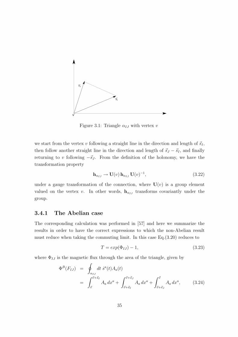
Figure 3.1: Triangle αIJ with vertex v
we start from the vertex v following a straight line in the direction and length of ~sI ,
then follow another straight line in the direction and length of ~sJ − ~sI , and finally
returning to v following −~sJ . From the definition of the holonomy, we have the
transformation property
hαIJ→ U(v)hαIJ
U(v)−1, (3.22)
under a gauge transformation of the connection, where U(v) is a group element
valued on the vertex v. In other words, hαIJtransforms covariantly under the
group.
3.4.1 The Abelian case
The corresponding calculation was performed in [57] and here we summarize the
results in order to have the correct expressions to which the non-Abelian result
must reduce when taking the commuting limit. In this case Eq.(3.20) reduces to
T = exp(ΦIJ)− 1, (3.23)
where ΦIJ is the magnetic flux through the area of the triangle, given by
ΦB(FIJ) =
∮
αIJ
dt sa(t)Aa(t)
=
∫ ~v+~sI
~v
Aa dxa +
∫ ~v+~sJ
~v+~sI
Aa dxa +
∫ ~v
~v+~sJ
Aa dxa, (3.24)
35
where the connection Aa(~x(s)) is now a commuting object.
The basic building block in (3.24) is
∫ ~v2
~v1
Aa(~x) dxa =
∫ 1
0
Aa(~v1 + t (~v2 − ~v1)) (~v2 − ~v1)a dt
=
∫ 1
0
Aa(~v1 + t ~∆) ∆a dt
=
(1 +
1
2!∆b∂b +
1
3!(∆b∂b)
2 + . . .
)∆aAa(v), (3.25)
with ∆a = (~v2 − ~v1)a. The infinite series in parenthesis is
F (x) = 1 +1
2!x +
1
3!x2 +
1
4!x3 + · · · = ex − 1
x, (3.26)
yielding ∫ ~v2
~v1
Aa(~x) dxa = F (∆a ∂a) (∆a Aa(~v1)) . (3.27)
In the following we employ the notation ∆a Va = ~∆ · ~V . Using the above result in
the three integrals appearing in (3.24) and after some algebra, we obtain
ΦB(FIJ) = F1(~sI · ∇, ~sJ · ∇) saJ sb
I (∂a Ab(~v)− ∂b Aa(~v))
= F1(~sI · ∇, ~sJ · ∇) saJ sb
I εabcBc(v), (3.28)
where the gradient acts upon the coordinates of ~v. The function F1 is
F1(x, y) =y(ex − 1)− x(ey − 1)
x y (y − x)= −
∞∑n=1
1
(n + 1)!
xn − yn
x− y. (3.29)
Let us emphazise that F1(x, y) is just a power series in the variables x and y.
Expanding in powers of the segments saI we obtain
ΦB(FIJ) =
(1 +
1
3(sc
I + scJ) ∂c +
1
12(sc
I sdI + sc
I sdJ + sc
J sdJ) ∂c ∂d + ...
)×
× 1
2sa
IsbJεabcB
c(v). (3.30)
Notice that the combination
1
2sa
IsbJεabc = A nc, (3.31)
36
is just the oriented area of the triangle with vertex v and sides scI , sc
J , joining at
this vertex, having value A and unit normal vector nc.
To conclude we have to calculate
(eΦB(FIJ (∆)) − 1
)=
∞∑n=2
1
n!(ΦB(FIJ))n =
∞∑n=2
MnIJ(∆), (3.32)
where the subindex n labels the corresponding power in the vectors sa. The results
are
M2IJ(∆) := saIs
bJ
1
2!Fab, (3.33)
M3IJ(∆) := saIs
bJ
1
3!(xI + xJ)Fab, (3.34)
M4IJ(∆) := saIs
bJ
1
4!(x2
I + xIxJ + x2J)Fab + sa
IsbJsc
IsdJ
1
8FabFcd, (3.35)
M5IJ(∆) := saIs
bJsc
IsdJ
[1
4 · 3!(xI + xJ)FabFcd +
1
4 · 3!Fab(xI + xJ)Fcd
](3.36)
up to fifth order. We are using the notation xI = ~sI · ∇ = saI ∂a.
We expect that the non-Abelian generalization of the quantities (3.85), (4.52),
(3.35), (3.36) is produced by the replacement
Aa → Aa = Aρa Gρ, ∂a → Da = ∂a − [Aa, ] (3.37)
Fab → Fab = ∂aAb − ∂bAa − [Aa,Ab] (3.38)
Nevertheless, at this level there are potential ordering ambiguities which will be
resolved in the next subsections.
3.4.2 The non-Abelian case
In a similar way to the Abelian case we separate the calculation of the holonomy
hαIJin three basic pieces through the straight lines along the sides of the triangle
αIJ . We have
hαIJ= P (eL3)P (eL2)P (eL1) ≡ U3 U2 U1, (3.39)
37
where
L1 =
∫ 1
0
dtAa(~v + t ~sI) saI (3.40)
L2 =
∫ 1
0
dtAa(~v + ~sI + t (~sJ − ~sI)) (saJ − sa
I) (3.41)
L3 =
∫ 1
0
dtAa(~v + ~sJ − t ~sJ) (−saJ) (3.42)
Here we have parameterized each segment with 0 ≤ t ≤ 1.
Let us consider in detail the contribution
U1 = P (eL1), L1 =
∫ 1
0
dtAa(~v + t ~sI) saI , (3.43)
with ~sI = saI.
Using the definition
U1 = 1 +
∫ 1
0
dtAa(~v + t~sI)saI +
∫ 1
0
dt
∫ t
0
dt′Aa(~v + t~sI)Ab(~v + t′~sI)saIs
bI
+
∫ 1
0
dt
∫ t
0
dt′∫ t′
0
dt′′AaAbAcsaIs
bIs
cI + . . . , (3.44)
for the path ordering, we arrive at the following expression
U1 = 1 + I1(x)Aa(v)saI + I2(x, x)Aa(v)Ab(v)sa
IsbI
+I3(x, x, ¯x)Aa(v)Ab(v) ¯Ac(v)saIs
bIs
cI + . . . (3.45)
Here we are using the conventions
x = scI∂c x = sc
I ∂c ¯x = scI¯∂c (3.46)
I1(x) = F (x), I2(x, x) =F (x + x)− F (x)
x(3.47)
I3(x, x, ¯x) =1¯x
[1
x + ¯x(F (x + x + ¯x)− F (x))− 1
x(F (x + x)− F (x))
](3.48)
with F (x) given by Eq.(3.26). The notation in Eq. (3.45) is that each operator
x, x, ¯x acts only in the corresponding field A, A, ¯A respectively. We write
U1 =∑N
U(N)1 , (3.49)
38
where the superindex N indicates the powers of saI contained in each term. A
detailed calculation produces
U(1)1 = sa
IAa, U(2)1 =
1
2(xsa
IAa + saIs
bIAaAb) (3.50)
U(3)1 =
1
3!(x2sa
IAa + (x + 2x)saIs
bIAaAb + sa
IsbIs
cIAaAbAc) (3.51)
U(4)1 =
1
4!
[x3sa
IAa + (3x2 + 3xx + x2)saIs
bIAaAb + (3x + 2x + ¯x)sa
IsbIs
cIAaAb
¯Ac
+saIs
bIs
cIs
dIAaAbAcAd
](3.52)
Now we put the remaining pieces together in order to calculate hαIJ= U3U2U1.
Using the notation
y = saJ ∂a (3.53)
and starting from the basic structure (3.45) we obtain, mutatis mutandis,
U(1)2 = (sa
J − saI)Aa, (3.54)
U(2)2 =
1
2[(x + y)(sa
J − saI)Aa + (sa
J − saI)(s
bJ − sb
I)AaAb], (3.55)
U(3)2 =
1
3![(x2 + y2 + xy)(sa
J − saI)Aa + (x + 2y + y + 2x)(sa
J − saI)(s
bJ − sb
I)AaAb
+ (saJ − sa
I)(sbJ − sb
I)(scJ − sc
I)AaAbAc)], (3.56)
U(4)2 =
1
4![(x3 + y3 + x2y + xy2)(sa
J − saI)Aa + (xy + 3xx + x2 + 2xy + 2xy + 3x2 + 3y2 + y2 +
+ 3yy + 5xy)(saJ − sa
I)(sbJ − sb
I)AaAb + (x + 2x + 3¯x + 2y + ¯y + 3y)(saJ − sa
I)
× (sbJ − sb
I)(scJ − sc
I)AaAb¯Ac + (sa
J − saI)(s
bJ − sb
I)(scJ − sc
I)(sdJ − sd
I)AaAbAcAd] (3.57)
for U2, together with
U(1)3 = −sa
JAa, (3.58)
U(2)3 =
1
2(−ysa
JAa + saJsb
JAaAb), (3.59)
U(3)3 =
1
3!(−y2sa
JAa + (2y + y)saJsb
JAaAb − saJsb
JscJAaAbAc), (3.60)
U(4)3 =
1
4!
[−y3sa
JAa + (3y2 + 3yy + y2)saJsb
JAaAb − (3¯y + 2y + y)saJsb
JscJAaAb
¯Ac
+saJsb
JscJsd
JAaAbAcAd
], (3.61)
39
for U3. Let us emphasize that in all the expressions above for U1, U2 and U3, the
connection is evaluated at the vertex v. The bars only serve to indicate the position
in which the corresponding derivative acts.
Next we write the contributions to the holonomy in powers of the segments. We
obtain
h(2)αIJ
=1
2sa
IsbJ Fab, (3.62)
h(3)αIJ
=1
3!(sc
I + scJ)sa
IsbJDcFab, (3.63)
h(4)αIJ
=1
4!(sc
IsdI + sc
IsdJ + sc
JsdJ)sa
IsbJDcDdFab +
1
8sa
IsbJsc
IsdJFabFcd. (3.64)
Eq. (3.64) resolves the ordering ambiguity which apparently arises in covariantizing
the first term in the RHS of Eq.(3.35). Nevertheless, as we subsequently show there
is no such ambiguity at this order. Let us consider the combination
saIs
bJsc
IsdJ (DcDd −DdDc)Fab = sa
IsbJsc
IsdJ [Dc,Dd]Fab
= −saIs
bJsc
IsdJ [Fcd,Fab] = [F,F] = 0 (3.65)
where we have used the notation F = saIs
bJFab together with the property
[Dc,Dd]G = − [Fcd,G] (3.66)
valid for any object G in the adjoint representation.
The results (3.62), (3.63) and (3.64), which we have obtained by direct calcula-
tion, constitute in fact the unique gauge covariant generalization of the correspond-
ing Abelian expressions (3.85), (4.52) and (3.35). This provides a strong support to
our method of calculation.
3.5 Electric flux expansion
Now we turn to the electric piece of the regularization. The basic covariant object
involved in the expression (3.18) is
40
F = he+ρ(p) E(p) h−1e+ρ(p) (3.67)
In order to simplify the calculation, we will consider the path ρ(p) connecting
the vertex v to the point p to be a straight line x.
Recalling from the expression (3.45), we can write
hv+sI= 1 +
[I1(x)A + I2(x, x)AA + I3(x, x, ¯x)AA ¯A + . . .
](v) (3.68)
where the notation is such that A = xaAa and the same definitions as before.
Considering the inverse operator h−1v+x, defined as the operator along the inverse
path, which amounts the replacement A → −A and the cyclic permutation that
takes into consideration a proper ordering of x′ segments, it follows
h−1v+x = [1− I1(x)A + I2(x, x)AA− I3(¯x, x, x)AA ¯A + . . . ](v) (3.69)
Taking into account the fact that hv+xh−1v+x = 11 and the explicit form of the I’s
expressions, we get
I2(x, x) + I2(x, x) = I1(x)I1(x) (3.70)
and
I1(¯x)I2(x, x)− I1(x)I2(x, ¯x) = I3(¯x, x, x)− I3(x, x, ¯x) (3.71)
and the permutations (x, x) → (x, x). Together with
I3(x, ¯x, x) + I3(¯x, x, x) + I3(¯x, x, x) = I1(x)I2(¯x, x) (3.72)
and the permutations (x, ¯x) → (¯x, x).
After a tricky manipulation we find the the compact equation with a clear ten-
dency,
41
F = hv+xE(v + x)h−1v+x = E− I1(x)[A, E] + I2(x, x)[ A, [ A, E] ] +
−I3(x, x, ¯x)[
¯A, [ A, [ A, E ] ]]
+ . . . (3.73)
Which results to be
F ≈
E + DE +1
2!D2E +
1
3!D3E + . . .
(v) (3.74)
Where again the notation is D = xaDa, and Da the covariant derivative
3.6 Semiclassical analysis: A general scheme
The corresponding modifications to the Yang Mills theory requires now to resolve
the last technical and conceptual problem. For the sake of clarity, let us resume
what has been done and to describe the calculations which would take place next.
The Yang Mills Hamiltonian has been regularized, with little deviation from the
original work [51]. It is now written in terms of the volume operator and in terms
of matter fields operators ready for the semiclassical approximation. The volume
operator has arise as a natural regulator of QFT acting exclusively on vertex points
of the graph introduced by the state.
The problem we are left in now, is to the search for good semiclassical states that
could approximate a flat geometry. A flat space is the geometry we are requiring
for our effective theory to live on. There has been extensive deal of attention in the
problem of semiclassical loop gravity [69, 70, 71, 72, 73, 74, 75, 76, 77], in particular
because the problem is tightly interlaced with one of the open problems in the LQG
approach. The problem is how to recover the classical geometry solely from quantum
properties of space. The analogy is close of the one faced when trying to reobtain
the classical properties of liquids from the quantum molecular theory.
In the calculations of expectations values of regularized Hamiltonian, we will
choose semiclassical states picked around a three metric with the properties de-
scribed in [57]. However, these are not the correct semiclassical states neither the
42
so called weave states, since they not fulfill peakedness properties around the con-
nection, which relies on the more fundamental problem described above.
Taking into account the expression for the regularized Hamiltonian, let us sepa-
rate the operator in gravitational and matter components as,
H[N ] =∑
v, ∆, ∆′εJKLεMNP wi L ∆(e)wi P ∆(e′)HI
∆JK(e)HI∆′MN(e′) (3.75)
where
wi L ∆(e) = tr
(τi heL(∆)
[h−1
eL(∆),
√Vv
])(3.76)
The magnetic contribution have the structure
HI∆JK(e) = εabce
aJeb
K ×[
1
2!Bc
I +1
3!(sd
J + sdK)DdB
cI +
1
4!(sf
JsdJ + sf
JsdK + sf
KsdK)DfDdB
cI
+1
8sf
JspKεfpdεI L M Bd
LBcM + . . .
](v) (3.77)
The electric part is analogous but considering only at linear order in the field,
also with modifications in some coefficients calculated in the appendix A.
To proceed with the approximation we think of space as made up of boxes,
each centered at a given point ~x and with volume L3 ≈ d3 x. Each box is defined
to contain a large number of vertices of the semiclassical state (L >> `P ), but
infinitesimal in the scale where the space can be regarded as continuous. Also, we
assume that the magnetic operators are slowly varying inside the box (`P << λD),
in such a way that for all the vertices inside the box one can write
〈W, ~E, ~B| . . . BaI (v) . . . |W, ~E, ~B〉 = µBa
I (~x). (3.78)
Here B is the classical magnetic field at the center of the box and µ is a di-
mensionless constant to be determined in such a way that we recover the standard
classical result (3.19) in the zeroth order approximation. In the next subsection we
show that
µ =
( L`P
)1+Υ
, (3.79)
43
with Υ being a parameter defining the leading order contribution of the gravitational
connection to the expectation value. Applying to (3.75) the procedure just described
leads to
H =∑Box
N(~x)
[BI
a1(~x)BI
b1(~x)
∑v∈Box
εJKLεMNP < W, ~E, ~B| Q∆L(e)Q∆′P (e′)×
× εa1a2a3 × εb1b2b3 × eJa2
eKa3
e′Mb2 e′Nb3 |W, ~E, ~B > +BIa1
(~x)DpBIb1
(~x)∑
v∈Box
εJKL × εMNP
× < W, ~E, ~B| Q∆L(e)Q∆′P (e′)εa1a2a3 × εb1b2b3eJa1
eKa2
e′Mb2 e′Nb3 (e′Mp + e′Np )|W, ~E, ~B > +
DqBIa1
(~x)DpBIb1
(~x)∑
v∈Box
εJKLεMNP ×
× < W, ~E, ~B| Q∆L(e)Q∆′P (e′)eJa2
eKa3
(eJq + eK
q )e′Mb2 e′Nb3 (e′Mp + e′Np )|W, ~E, ~B >
+ . . . ] (3.80)
The general structure is
HB =∑Box
N(~x)BIr1
(~x) . . . BIrn
(~x)(Da1 . . . DamBI
r (~x))
d3x Ra1...am
rr1...rn(~x)
HB =
∫d3x N(~x)BI
r1(~x) . . . BI
rn(~x)
(Da1 . . . Dam BI
r(~x))
Ra1...am
rr1...rn(~x)
(3.81)
R is constructed from flat space tensors like δab, εabc. In this way we are demand-
ing covariance under rotations at the scale L.
When averaging inside each box, the scaling of the expectation values of the
gravitational operators is estimated according to
〈W, ~E, ~B | . . . Aia . . . |W, ~E, ~B 〉 ≈ . . .1
L(
`P
L)Υ
. . . , (3.82)
〈W, ~E, ~B | . . .√
Vv . . . |W, ~E, ~B 〉 ≈ . . . `3/2P . . . , (3.83)
44
3.7 Yang Mills effective Hamiltonian
In constructing the effective theory we will put all the elements of the previous
sections altogether, and note that the following calculation of elements R has been
already calculated in [57].
Let us now continue with the calculation of the contribution to (3.17) due to the
magnetic flux by writing the expansion
tr(τIhαJK) = tr
(τI
∞∑n=2
h(n)αJK
)= M I
2JK(∆) + M I3JK(∆) + M I
4JK(∆)
+O (s5F 4
)(3.84)
where
M I2IJ(∆) := sa
IsbJ
i
2!F I
ab (3.85)
M I3IJ(∆) := sa
IsbJ
i
3!(xI + xJ)F I
ab − saIs
bJsc
IsdJεI L M 1
8FL
abFMcd (3.86)
M I4JK(∆) := sa
KsbJ
i
4!(x2
J + xJxK + x2K)F I
ab (3.87)
and BIc = εabcF I
ab
according to the previous analysis. We are using the notation xI = ~sI · ~D = saI Da.
Let us remark that, contrary to the electric case, the magnetic contribution will
incorporate non-linear terms due to the expansion of the exponential in powers of~B. This implies that the exact duality symmetry of Maxwell equations in vacuum
will be lost due to quantum gravity corrections.
Next let us consider the gravitational contributions to (3.18), arising from the
gravitational part of (3.76), which we expand as
wi L∆ = saLwia + sa
LsbLwiab + sa
LsbLsc
Lwiabc +O(s4w), (3.88)
with
wia =1
2[Aia,
√V ], wiab =
1
8εijk[Aja, [Akb,
√V ]], wiabc = − 1
48[Aja, [Ajb, [Aic,
√V ]]].(3.89)
45
The scaling properties of the above gravitational operators under the semiclassical
expectation value are
〈W ~E ~B| . . . wi a1...an . . . |W ~E ~B〉 → `P3/2
Ln
(`P
L)nΥ
. (3.90)
For the product wi L∆wi P∆′ we need only
wi L∆wi P∆′ = U2LP + U3LP + U4LP +O (s5w2
)(3.91)
with
U2LP = saLs′dP wiawid,
U3LP = saLs′dP s′eP wiawide + sa
LsbLs′dP wiabwid,
U4LP = saLs′dP s′eP s′fP wiawidef + sa
LsbLs′dP s′eP wiabwide + sa
LsbLsc
Ls′dP wiabcwid. (3.92)
Here all the w’s are evaluated at a common vertex v.
At this level it is convenient to state the result (no sum over L)
saL sb
L wiab =1
8sa
L sbL εijk [Aja, [Akb,
√V ]]
=1
8sa
L sbL εijk
(AjaAkb
√V − Aja
√V Akb − Akb
√V Aja +
√V AkbAja
),
= 0, (3.93)
which holds due to symmetry properties. This leads to
U3LP = 0. (3.94)
After taking the expectation value the terms contributing to order `2P
T = T0 + T1 + T2 +O(→ `3P ) (3.95)
T0 = − 1
2 Q2
1
`4P
εJKL εMNP[U2LP M I
1JK M ′I1MN
], (3.96)
T1 = − 1
2 Q2
1
`4P
εJKL εMNP U2LP
[M I
1JK M ′I2MN + M I
2JK M ′I1MN
], (3.97)
T2 = − 1
2 Q2
1
`4P
εJKL εMNP[
U2LP (M I1JK M ′I
3MN + M I3JK M ′I
1MN + M2JK M ′2MN) +
+U4LP M I1JK M ′I
1MN
]. (3.98)
46
Now we are ready to calculate the different contributions to the magnetic sector
of the Hamiltonian (3.18). The task is to calculate the R pieces which are symmetric
in the indices r1, r2, . . . , rn. The first contribution to To is
R0r1r2 =
∑v∈Box
1
2Q2
(2
3!
8
E(v)
)2 ∑
v(∆)=v(∆′)=v
µ2
4 `7P
εr1ab εr2
uv εJKL εMNP ×
× saK sb
J scL s′vM s′uN s′dP 〈W ~E ~B|wic wid |W ~E ~B〉. (3.99)
And with the relations
εKJL saK sb
J scL = det(s) εabc, det(s) = det(sa
K), εabpεabq = 2δpq . (3.100)
(3.99) can be rewriten in the simpler form
R0r1r2 =
∑v∈Box
1
2 Q2
(2
3!
8
E(v)
)2 ∑
v(∆)=v(∆′)=v
µ2
`7P
×
× det(s) det(s′) 〈W, ~E, ~B|12wi
r1 , wir2 |W, ~E, ~B〉. (3.101)
The above equation implies
R0r1r2 =
1
2 Q2
µ2
`7P
`6P
`3P
L2
(`P
L)2Υ
δr1r2 =1
2 Q2δr1r2 , (3.102)
which reproduces the zeroth-order magnetic contribution (3.19) with the choice
µ =
( L`P
)1+Υ
. (3.103)
The contribution to the T ′s have been calculated in the previous work [57]. Let
us just write them
The correction arising from T1 is
R11a1rr1 = κ8
µ2
Q2 `7P
`7P
`3P
L2
(`P
L)2Υ
εa1rr1 , (3.104)
47
which produces a parity-violating term in the magnetic sector of the effective
Hamiltonian.
The next contribution arises from T2 and can be separated into three pieces
HB21 =
∑
v∈V (γ)
1
2 Q2
(2
3!
8
E(v)
)2
`3P
∑
v(∆)=v(∆′)=v
− 1
`7P
εJKL εMNP ×
×〈W, ~E, ~B|U2LP (M I1JK M ′I
3MN + M I3JK M ′I
1MN) |W, ~E, ~B〉, (3.105)
HB22 =
∑
v∈V (γ)
1
2 Q2
(2
3!
8
E(v)
)2
`3P
∑
v(∆)=v(∆′)=v
− 1
`7P
εJKL εMNP ×
×〈W, ~E ~B|U2LP M I2JK M ′I
2MN |W, ~E, ~B〉, (3.106)
HB23 =
∑
v∈V (γ)
1
2 Q2
(2
3!
8
E(v)
)2
`3P
∑
v(∆)=v(∆′)=v
− 1
`7P
εJKL εMNP ×
×〈W, ~E, ~B|U4LP M I1JK M ′I
1MN |W, ~E, ~B〉. (3.107)
Let us start discussing HB21. After some algebra we obtain
HB21 =
∑
v∈V (γ)
1
2 Q2
(2
3!
8
E(v)
)2
`3P
∑
v(∆)=v(∆′)=v
− i
`7P
εJKL εMNP ×
× saLs′dP s′xNs′qM 〈W, ~E, ~B|wiawid
(sr
KstJ
i
4!(x2
J + xJxK + x2K)F I
rt
)F I
xq |W, ~E, ~B〉,(3.108)
which naturally splits into the following pieces
HB211 =
∑
v∈V (γ)
1
2 Q2
(2
3!
8
E(v)
)2
`3P
∑
v(∆)=v(∆′)=v
− i
`7P
εJKL εMNP ×
× saLs′dP s′xNs′qM 〈W, ~E, ~B|wiawid
(sr
KstJ
i
4!(x2
J + xJxK + x2K)F I
rt
)F I
xq |W, ~E, ~B〉,(3.109)
48
The corresponding R tensors are
R211a1a2rr1 =
∑v∈Box
1
2
(2
3!
8
E(v)
)2 ∑
v(∆)=v(∆′)=v
2 µ2
4! Q2`7P
det(s′)det(s)
εNKJ
(s−1
)rNεJKL sa
L (2sa1J sa2
J + sa1J sa2
K ) 〈W, ~E, ~B|wiawr1
i |W, ~E, ~B〉,
R211a1a2rr1 =
µ2
Q2`7P
`8P
`3P
L2
(`P
L)2Υ (
κ6 δa1a2 δrr1 + κ7 (δa1r δa2r1 + δa2r δa1r1))
,(3.110)
Now we continue with the correction arising from (3.106), which reduces to
HB22 =
∑v∈Box
1
2 Q2
(2
3!
8
E(v)
)2
`3P
∑
v(∆)=v(∆′)=v
4
(3!)2 `7P
εJKL εMNP ×
×saLs′dP 〈W, ~E, ~B|wiawid
(su
KsyJ xJF I
uy
) (s′rNs′sM x′MF I
rs
) |W, ~E, ~B〉,(3.111)
Then
R22a1a2rr1 =
∑v∈Box
1
2 Q2
(2
3!
8
E(v)
)2 ∑
v(∆)=v(∆′)=v
4 µ2
(3!)2 `7P
det(s)det(s′)×
× (−εY MNεPMNs′dP s′a2M
) (εXJKεLJK sa
L sa1J
) (s−1
)Xr1(s′−1
)Y r
×〈W, ~E, ~B|wiawid |W, ~E, ~B〉. (3.112)
where we have used the relation
εmbc sbJ sc
L = det(s) εKJL
(s−1
)K
m, (3.113)
we find
R22a1a2rr1 =
µ2
Q2`7P
`8P
`3P
L2
(`P
L)2Υ (
κ9 δa1a2 δrr1 + κ10 (δa1r δa2r1 + δa2r δa1r1))
.
(3.114)
This contribution is of the same kind as the one given by R211a1a2rr1 .
Finally we are left with
49
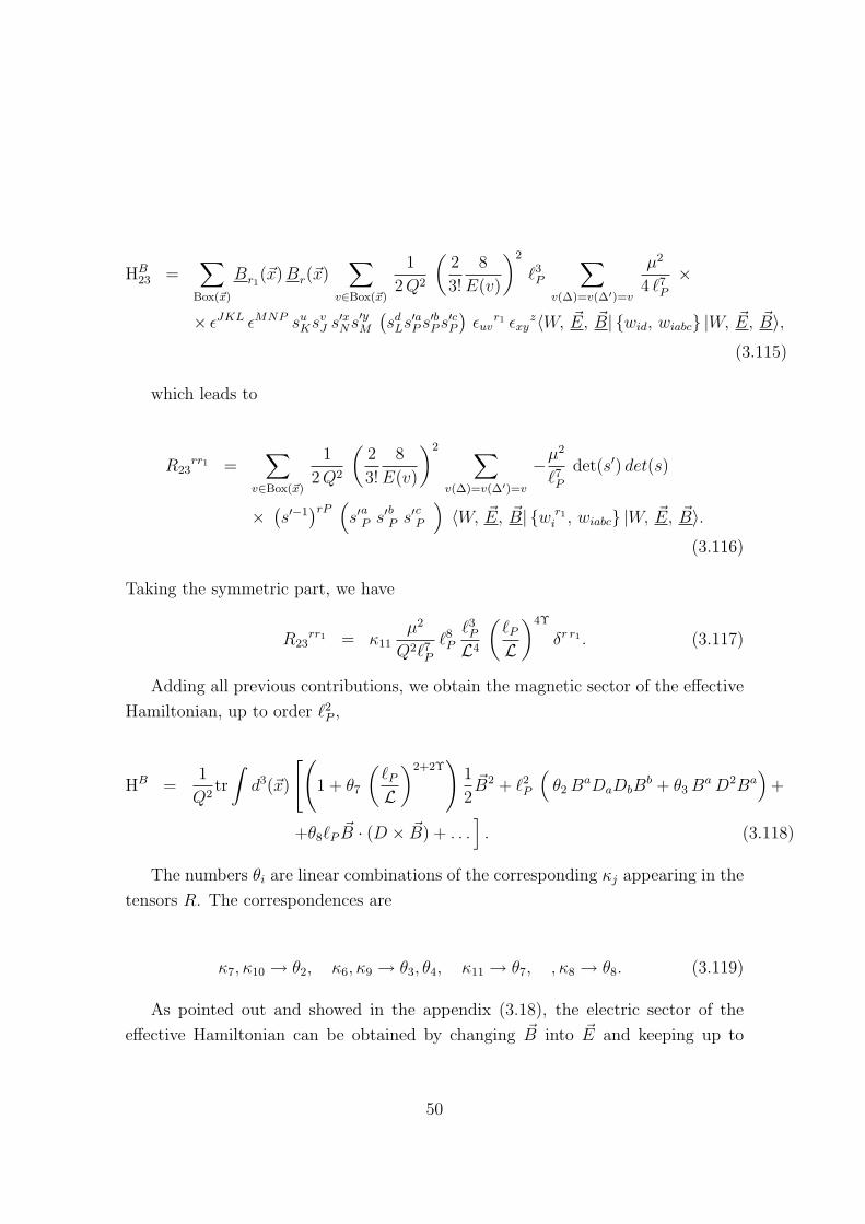
HB23 =
∑
Box(~x)
Br1(~x) Br(~x)
∑
v∈Box(~x)
1
2 Q2
(2
3!
8
E(v)
)2
`3P
∑
v(∆)=v(∆′)=v
µ2
4 `7P
×
× εJKL εMNP suKsv
J s′xNs′yM(sd
Ls′aP s′bP s′cP)
εuvr1 εxy
z〈W, ~E, ~B| wid, wiabc |W, ~E, ~B〉,(3.115)
which leads to
R23rr1 =
∑
v∈Box(~x)
1
2 Q2
(2
3!
8
E(v)
)2 ∑
v(∆)=v(∆′)=v
−µ2
`7P
det(s′) det(s)
× (s′−1
)rP(s′aP s′bP s′cP
)〈W, ~E, ~B| w r1
i , wiabc |W, ~E, ~B〉.(3.116)
Taking the symmetric part, we have
R23rr1 = κ11
µ2
Q2`7P
`8P
`3P
L4
(`P
L)4Υ
δr r1 . (3.117)
Adding all previous contributions, we obtain the magnetic sector of the effective
Hamiltonian, up to order `2P ,
HB =1
Q2tr
∫d3(~x)
[(1 + θ7
(`P
L)2+2Υ
)1
2~B2 + `2
P
(θ2 BaDaDbB
b + θ3 Ba D2Ba)
+
+θ8`P~B · (D × ~B) + . . .
]. (3.118)
The numbers θi are linear combinations of the corresponding κj appearing in the
tensors R. The correspondences are
κ7, κ10 → θ2, κ6, κ9 → θ3, θ4, κ11 → θ7, , κ8 → θ8. (3.119)
As pointed out and showed in the appendix (3.18), the electric sector of the
effective Hamiltonian can be obtained by changing ~B into ~E and keeping up to
50
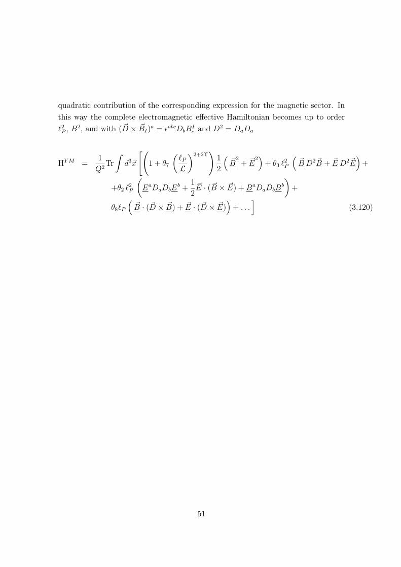
quadratic contribution of the corresponding expression for the magnetic sector. In
this way the complete electromagnetic effective Hamiltonian becomes up to order
`2P , B2, and with ( ~D × ~BI)
a = εabcDbBIc and D2 = DaDa
HY M =1
Q2Tr
∫d3~x
[(1 + θ7
(`P
L)2+2Υ
)1
2
(~B
2+ ~E
2)
+ θ3 `2P
(~B D2~B + ~E D2~E
)+
+θ2 `2P
(EaDaDbE
b +1
2~E · ( ~B × ~E) + BaDaDbB
b
)+
θ8`P
(~B · ( ~D × ~B) + ~E · ( ~D × ~E)
)+ . . .
](3.120)
51
Chapter 4
Higgs effective model
In the following chapter the goal we pursue is to obtain the corresponding modifica-
tions to the Higgs field, which will be carried using the same techniques developed
in the Yang Mills case. The Higgs field remains the last unexplored sector of the
SM [56, 57].
In the derivation of the Higgs effective theory we will shift from the usual vari-
ables to new ones, which are the smeared in space momentum and the adimensional
point holonomy variable. The main reason in doing so, is that the new variables
allows to implement correctly the adjointness relations, which are not trivially im-
plemented for diffeomorphism invariant field theories (a complete discussion can be
found in [85]
52
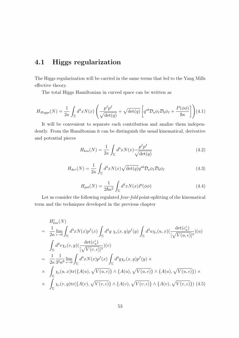
4.1 Higgs regularization
The Higgs regularization will be carried in the same terms that led to the Yang Mills
effective theory.
The total Higgs Hamiltonian in curved space can be written as
HHiggs(N) =1
2κ
∫
Σ
d3xN(x)
(pIpI
√det(q)
+√
det(q)
[qabDaφIDbφI +
P (φφ)
~κ
])(4.1)
It will be convenient to separate each contribution and analize them indepen-
dently. From the Hamiltonian it can be distinguish the usual kinematical, derivative
and potential pieces
Hkin(N) =1
2κ
∫
Σ
d3xN(x)pIpI
√det(q)
(4.2)
Hder(N) =1
2κ
∫
Σ
d3xN(x)√
det(q)qabDaφIDbφI (4.3)
Hpot(N) =1
2~κ2
∫
Σ
d3xN(x)P (φφ) (4.4)
Let us consider the following regulated four-fold point-splitting of the kinematical
term and the techniques developed in the previous chapter
Hεkin(N)
=1
2κlimε→0
∫
Σ
d3xN(x)pI(x)
∫
Σ
d3y χε(x, y)pI(y)
∫
Σ
d3uχε(u, x)(det(ei
a)
[√
V (u, ε)]3)(u)
∫
Σ
d3vχε(v, y)(det(ei
a)
[√
V (v, ε)]3)(v)
=1
2κ
1
32κ6limε→0
∫
Σ
d3xN(x)pI(x)
∫
Σ
d3yχε(x, y)pI(y)×
×∫
Σ
χε(u, x)tr(A(u),√
V (u, ε) ∧ A(u),√
V (u, ε) ∧ A(u),√
V (u, ε))×
×∫
Σ
χε(v, y)tr(A(v),√
V (v, ε) ∧ A(v),√
V (v, ε) ∧ A(v),√
V (v, ε)) (4.5)
53
Recall that∫
d3x det(eia) = 1
3!
∫εijke
i ∧ ej ∧ ek = −13
∫tr(e ∧ e ∧ e).
Let us define
Q[χ] :=
∫
Σ
χε(u, x)tr(A(u),
√V (u, ε) ∧ A(u),
√V (u, ε) ∧ A(u),
√V (u, ε)
)
=∑∆
∫
∆
χε(u, x)tr(A(u),
√V (u, ε) ∧ A(u),
√V (u, ε) ∧ A(u),
√V (u, ε)
)
Q[χ] =∑∆
Q∆[χ]. (4.6)
Where we have defined
Q∆[χ] =
∫
∆
χε(u, x)tr(A(u),
√V (u, ε) ∧ A(u),
√V (u, ε) ∧ A(u),
√V (u, ε)
)(4.7)
And let us define the gauge invariant object pI(Be) by,
pI(Be) := tr
[τIhe
(∫
Be
hρ(r)p(r)h−1ρ(r)d
3x(r)
)h−1
e
](4.8)
Where hρ(r) is the parallel propagator from the vertex v to the point r in the
region Be
Now consider the three vectors saJ(∆)sb
K(∆)scL(∆) that span the tetrahedra ∆
with base in e = v, we have
pI(Bv) =1
3!εJKLεabcsa
JsbKsc
LpI(v) +
+1
4!εJKLεabcsa
JsbKsc
L(saJ + 2sa
I + saK)Dap(v) + O(s5) (4.9)
Therefore for a small tetrahedra ∆
f(v)pI(Bv) =1
3!f(v)εJKLεabcsa
JsbKsc
LpI(v) + Dap(v) =
∫
Bv
d3xf(x)pI(x) (4.10)
And considering
54
∫
∆
tr(A(x),
√V (x, ε) ∧ A(x),
√V (x, ε) ∧ A(x),
√V (x, ε))
≈ 1
3!εIJKtr(hsI(∆)h−1
sI(∆),
√V (v(∆), ε)tr(hsJ (∆)h−1
sJ (∆),
√V (v(∆), ε) ×
× tr(hsK(∆)h−1sK(∆),
√V (v(∆), ε)) (4.11)
We have then for the familiar triangulation,
Q∆ =1
3!εIJKtr(hsI(∆)h−1
sI(∆),√
V (v(∆), ε)tr(hsJ (∆)h−1sJ (∆),
√V (v(∆), ε) ×
× tr(hsK(∆)h−1sK(∆),
√V (v(∆), ε)) (4.12)
And we rewrite
Hεkin(N) =
1
2κ732limε→0
∑
pqrs∈V (γ)
N(p)pI(Bp)pI(Bq)χ(p, q)×
× 8
E(r)χ(r, p)
∑
v(∆)=r
Q∆8
E(s)χ(s, q)
∑
v(∆′)=s
Q∆′ (4.13)
Now we replace the classical objects by their quantum counterpart and we take
the limit. Now we just take ε to zero, realize that only terms with v = p = q = r = s
contribute and find that,
Hkin[N ] =1
2κ732(i~)6
∑
v∈V (γ)
N(v)
(8
E(v)
)2
pI(Bv)pI(Bv)×
×∑
v(∆)=v(∆′)=v
εIJKεLMNtr(hsI(∆)[h−1sI(∆),
√V (v(∆), ε)]tr(hsJ (∆)[h
−1sJ (∆),
√V (v(∆), ε)]×
× tr(hsK(∆)[h−1sK(∆),
√V (v(∆), ε)])tr(hsL(∆′)[h
−1sL(∆′),
√V (v(∆′), ε)]×
× tr(hsM (∆′)[h−1sM (∆′),
√V (v(∆′), ε)])tr(hsN (∆′)[h
−1sN (∆′),
√V (v(∆′), ε)] (4.14)
now because only tetrahedra based at vertices γ contribute in the sum∫
σ=∑
∆
∫∆
55
Hkin[N ] =1
2κ732(i~)6
∑
v∈V (γ)
N(v)
(8
E(v)
)2
pI(Bv)pI(Bv)×
×∑
v(∆)=v(∆′)=v
εIJKεLMNtr(hsI(∆)[h−1sI(∆),
√Vv]tr(hsJ (∆)[h
−1sJ (∆),
√Vv]×
× tr(hsK(∆)[h−1sK(∆),
√Vv])tr(hsL(∆′)[h
−1sL(∆′),
√Vv]×
× tr(hsM (∆′)[h−1sM (∆′),
√Vv])tr(hsN (∆′)[h
−1sN (∆′),
√Vv] (4.15)
where B is a compact region in Σ, and E(v) is the usual function E(v) =
n(v)(n(v)− 1)(n(v)− 2) where n(v) is the valence of the vertex v.
Next we turn to the term containing the derivatives of the scalar field.
Then considering eq(4.3)
Hder[N ] =1
2κ
∫
Σ
d3xN(x)√
det(q)qabDaφIDbφI (4.16)
And with
qab√
det(q) =Ea
i Ebi√
det(q)and Ea
i = εacdεijkej
cekd
2
We write and regulate (again we could have chosen to replace only one of the Eai by
the term quadratic in eia and still would arrive at a well-defined result at the price
of losing symmetry of the expression).
Hder[N ]
=1
2κlimε→0
∫d3x
∫d3yN(x)χε(x, y)εijkεimnεabc (DaφIe
jbe
kc )(x)√
V (x, ε)εbef
(DbφIeme en
f )(y)√V (y, ε)
=1
2κ5(2
3)4 lim
ε→0
∫N(x)εijkDφI(x) ∧ Aj(x), V (x, ε)3/4 ∧ Ak(x), V (x, ε)3/4 ×
×∫
χε(x, y)εimnDφI(y) ∧ Am(x), V (y, ε)3/4 ∧ An(y), V (y, ε)3/4 . (4.17)
56
It is clear where we are driving at. We replace Poisson brackets by commutators
times 1/i~ and V by its operator version. Furthermore we introduce the already
familiar triangulation of Σ and have, using that with v = s(0) for some path s
Let us define the quantity
Γ[f ] =
∫
Σ
f(x)DφI(x) ∧ Aj(x), V (x, ε)3/4 ∧ Ak(x), V (x, ε)3/4
=∑∆
∫
∆
f(x)DφI(x) ∧ Aj(x), V (x, ε)3/4 ∧ Ak(x), V (x, ε)3/4 (4.18)
Then
Hder[N ] =1
2κ5(2
3)4 lim
ε→0
∑
∆∆′Γ∆[N ]Γ∆′ [χ] . (4.19)
Now the functional derivative of Φ(v) = eφIτI with respect to φI(x) turns out to
be meaningless without a regularization of Φ(v) as well.
In [85] a regularization which takes the interpretation of Φ(v) as the nontrivial
limit of a holonomy he as e shrinks to e serious has been used to take into account
a consistent implementation of the adjoint relations. We will use this variables
explained in that work.
We see that
hs(0, δt)Φ(s(δt))hs(0, δt)−1 − Φ(v)
= exp(hs(0, δt)φ(s(δt))hs(0, δt)−1)− Φ(v)
= exp([1 + δtsa(0)Aa][φ(v) + δtsa(0)∂aφ(v)][1− δtsa(0)Aa] + o((δt)2))− Φ(v)
= exp(δtsa(0)(∂aφ(v) + [Aa, φ(v)]) + o((δt)2))− U(v) = δtsa(0)Daφ(v) + o((δt)2),
(4.20)
And using the expression derived in the previous chapter, we arrive to
57
6
∫
∆
f(x)DφI(x) ∧ Aj(x), V (x, ε)3/4 ∧ Ak(x), V (x, ε)3/4
≈ −4
dεmnp f(v(∆)) tr(τ I [hv+sM
Φ(sM(∆))h−1v+sM
− Φ(v(∆))])×× tr(τjhsN (∆)h−1
sN (∆), V (v(∆), ε)3/4)tr(τkhsP (∆)h−1sP (∆), V (v(∆), ε)3/4) .(4.21)
and with tr(τiτj) = −δij/2, tr(τ IτJ) = −dδIJ , d the dimension of the fundamen-
tal representation of G that
Hder[N ] =1
2κ5~4(2
3)4(
2
3d)2 lim
ε→0
∑
v,v′∈V (γ)
N(v)χε(v, v′)εijkεilm ×
×∑
v(∆)=v
8
E(v)εNPQtr(τ I [hv+sN
Φ∆(sN)h−1v+sN
− Φ(v)])×
× tr(τjhsP (∆)[h−1sP (∆), V
3/4v ])tr(τkhsQ(∆)[h
−1sQ(∆), V
3/4v ])×
×∑
v(∆′)=v
8
E(v)εRST tr(τ I [hv+sR
Φ∆′(sR)h−1v+sR
− Φ(v)])×
× tr(τlhsS(∆′)[h−1sS(∆′), V
3/4v ])tr(τmhsT (∆′)[h
−1sT (∆′), V
3/4v ]) (4.22)
since only tetrahedra with vertices as basepoints contribute. Thus we find in the
limit ε → 0
Hder[N ] =1
2κ5~4(2
3)4(
2
3d)2
∑
v∈V (γ)
N(v)εijkεilm ×
×∑
v(∆)=v(∆′)=v
8
E(v)εNPQtr(τ I [hv+sN
Φ∆(sN)h−1v+sN
− Φ(v)])×
× tr(τjhsP (∆)[h−1sP (∆), V
3/4v ])tr(τkhsQ(∆)[h
−1sQ(∆), V
3/4v ])×
× εRST tr(τ I [hv+sRΦ∆′(sR)h−1
v+sR− Φ(v)])×
× tr(τlhsS(∆′)[h−1sS(∆′), V
3/4v ])tr(τmhsT (∆′)[h
−1sT (∆′), V
3/4v ]) (4.23)
Again, despite its complicated appearance, (4.23) defines a densely defined op-
erator.
58
Finally the potential term, is trivial to quantize. Notice that certain functions of
φI(v)φI(v) can be recovered from polynomials of the functions [tr(U(v)n)]m where
m,n are non-negative integers. Thus we may define for instance a mass term through
φi(v)2 := [arcos(tr(Φ(v))
2)]2
we find
Hpot(N) =mp
`3p
∑
v∈V (γ)
NvP (φIφI)(v)Vv (4.24)
This furnishes the quantization of the Higgs sector. Notice that the regularized
Hamiltonians have the same structure, namely an operator which carries out a dis-
crete operation on a spin network, divided by an appropriate power of the Planck
length which compensates the power of the Planck length coming from the action
of the volume operator.
4.2 Momentum and field covariant expansions
Let us now continue with the calculation of the contribution to (4.15) due to the
momentum integral by writing the expansion
pI(Bv) : = tr
[τIhv
(∫
Bv
hρ(r)p(r)h−1ρ(r)d
3x(r)
)h−1
v
](4.25)
And by using the expressions before
pI(Bv) : =~sI · (~sJ × ~sK)
3!
[pI(v) + T aDap
I(v) + T abDaDbpI(v) + . . .
](4.26)
where the T ′s can be calculated
T a =
∫
Bv
d3xxa =1
4(sa
J + 2saI + sa
K) (4.27)
59
T ab =
∫
Bv
d3xxaxb (4.28)
T a =1
4(sa
J + 2saI + sa
K) (4.29)
VB =~sI · (~sJ × ~sK)
3!(4.30)
=J
3!(4.31)
And for the derivative part
hv+sRΦ(sR)h−1
v+sR− Φ(v) = sa
RDaφ(v) +1
2!sa
RsbRDaDbφ(v) + . . . (4.32)
according to the previous analysis we are using the notation xI = ~sI · ~D = saI Da.
4.3 The Higgs effective Hamiltonian
Let us consider the total Higgs Hamiltonian without potential term
HHiggs = Hkin + Hder + Hpot (4.33)
The kinematical part is
Hkin[N ] =(−2)2
2κ7(3!)2(i~)6
∑
v∈V (γ)
N(v)
(8
E(v)
)2
p I(Bv)pI(Bv)×
×∑
v(∆)=v(∆′)=v
εIJKQI∆QJ∆QK∆ × εLMNQL∆′QM∆′QN∆′
(4.34)
60
and the derivative part is
Hder[N ] =1
2κ5~4(2
3)4(
2
3d)2
∑
v∈V (γ)
N(v)εijkεilm ×
×∑
v(∆)=v(∆′)=v
(8
E(v)
)2
εNPL tr(τI [hv+sN
Φ∆(sN)h−1v+sN
− Φ(v)])
QjP∆ QkL∆ ×
× εRST tr(τI [hv+sR
Φ∆′(sR)h−1v+sR
− Φ(v)])
QlS∆′ QmT∆′ (4.35)
Where
QI∆ = tr
(hsI(∆)[h
−1sI(∆),
√Vv]
)(4.36)
QiP∆ = tr(τihsP (∆)[h
−1sP (∆), V
3/4v ]
)(4.37)
4.3.1 Kinetic part
First we need to expand the relevant quantities taking part in (4.34)
pI(Bv) : =1
3!εpqrsp
IsqJsr
K
[pI(v) +
1
4(sa
J + 2saI + sa
K)DapI(v) + . . .
](4.38)
M I3IJK(∆) :=
1
3!εpqrsp
IsqJsr
KpI(v) (4.39)
M I4IJK(∆) :=
1
4!εpqrsp
IsqJsr
K(saJ + 2sa
I + saK)Dap
I(v) (4.40)
Next let us consider the gravitational contributions, which we expand as
QL∆ = saLsb
LQab + saLsb
LscLQabc +O(s4Q), (4.41)
with
61
Qab =1
4[Aia, [Aib,
√V ] ], Qabc =
1
24εijk[Aia, [Ajb, [Akc,
√V ] ] ]. (4.42)
The scaling properties of the gravitational operators under the semiclassical ex-
pectation value are
〈W ~E ~B| . . . Q a1...an . . . |W ~E ~B〉 → `P3/2
Ln
(`P
L)nΥ
. (4.43)
where we have used the same scaling for the connection see Eq.(3.83)
For the product Q I∆Q J∆QK∆ we need the element
Q I∆Q J∆QK∆ = U IJK2∆ + U IJK
3∆ +O (s4
)
(4.44)
where
U IJK2∆ = sa
IsbIs
cJsd
JseKsf
KQabQcdQef + saIs
bIs
cJsd
IseJsf
KsgKQabcQdeQfg
+O (s8
)(4.45)
U IJK3∆ = sa
IsbIs
cIs
dJse
JsfJsh
KsrKst
KQabcQdefQhrt +O (s10
)(4.46)
at this point all we need is to consider the tensorial structure and orders in the
segments more than the exhaustive analysis of the exact numerical coefficients since
they at last can be absorbed in the unknown coefficients coded at the end. Just to
see the structure of the terms they are roughly like
Therefore
Q I∆Q J∆QK∆QL∆′QM∆′QN∆′ = U IJK2∆ ULMN
2∆′ + U IJK3∆ ULMN
3∆′ +
+U IJK2∆ ULMN
3∆′ + U IJK3∆ ULMN
2∆′ +O(s7) (4.47)
62
We are considering
H =1
κ
∫d3xN(~x)p I(~x)
(Da1 . . . Da1p I(~x)
)Ra1...am(~x) (4.48)
T = T0 + T1 + T2 +O(→ `3P ) (4.49)
T0 =1
2κ632(i~)6εIJK εLMN
[U IJK
2∆ ULMN2∆′ M I
3IJ(∆)MI3LM(∆′)
],
T1 =1
2κ632(i~)6εJKL εMNP
[U IJK
2∆ ULMN2∆′
(M I
3IJ(∆)MI4LM(∆′) + M I
4IJ(∆)MI3LM(∆′)
)],
T2 =1
2κ632(i~)6εJKL εMNP
[M I
3IJ(∆)
(U IJK
2∆ ULMN3∆′ + U IJK
3∆ ULMN2∆′
) ].
The calculation is performed in the appendix.B , we are left with the kinetic
contribution to the Hamiltonian
Hkin =
∫d3x
2k
(p I p I + κ1`
2p
(DapI Dap
I)
+ κ2`3pε
abcDapI DbDcp
I) + . . .)
or
Hkin =
∫d3x
2kTr
[p · p + κ1`
2p
(~Dp · ~Dp
)+ κ2`
3p~Dp · ( ~D × ~Dp) + . . .
]
4.3.2 Derivative part
From the derivative part of the field we have the expansion
hv+sJΦ(sJ)h−1
v+sJ− Φ(v) = sa
RDaφ(v) +1
2!sa
JsbJDaDbφ(v) + . . . (4.50)
LI1J(∆) := sa
JDaφI(v) (4.51)
LI2J(∆) :=
1
2!sa
JsbJDaDbφ
I(v) (4.52)
LI3J(∆) :=
1
3!sa
JsbJsc
JDaDbDcφI(v) (4.53)
63
And the gravitational contributions of the derivative part of the Hamiltonian,
similarly as in the previous case the contributions are multiples of quantities like,
Qi L∆ = saLQia + sa
LsbLQiab + sa
LsbLsc
LQiabc +O(s4Q), (4.54)
with
Qia =1
2[Aia, V
3/4], Qiab =1
8εijk[Aja, [Akb, V
3/4]], Qiabc = − 1
48[Aja, [Ajb, [Aic, V
3/4]]].
(4.55)
For the product Qi P∆Qi L∆ we need the element
Qj P∆Qk L∆ = UPL jk2∆ + UPL jk
3∆ +O (s4
)
(4.56)
where
UPL jk2∆ = sa
P sbLQjaQkb + sa
P sbLsc
LQjaQkbc
+O (s8
)(4.57)
UPL jk3∆ = sa
P sbP sc
LscLQjabQkcd +O (
s10)
(4.58)
now all we need is to consider the tensorial structure and orders in the segments
more than the exhaustive analysis of the exact numerical coefficients since they at
last can be absorbed in the unknown coefficients coded at the end. Just to see the
structure of the terms they are roughly like
Therefore
Q iP∆Q jL∆Q lS∆′QmT∆′ = UPLij2∆ UST lm
2∆′ + UPL3∆ UST lm
3∆′ +
+UPLij2∆ UST lm
3∆′ + UPLij3∆ UST lm
2∆′ +O(s7) (4.59)
64
And
H =1
κ
∫d3xN(~x)Dr1φ
I(~x) . . .Drnφ I(~x) (Da1 . . . Dam)DrφI(~x) Rrr1...rn
a1...am(~x) (4.60)
K = K0 + K11 + K12 +O(→ `3P ) (4.61)
K0 =1
2κ4~4(2
3)4(
2
3d)2 εNPL εRST
[UPL
2∆ UST2∆′ L
I1N(∆)L
I1R(∆′)
],
K11 =1
2κ4~4(2
3)4(
2
3d)2 εNPL εRST
[UPL
2∆ UST2∆′
(LI
1N(∆)LI2R(∆′) + LI
2N(∆)LI1R(∆′)
)],
K12 =1
2κ4~4(2
3)4(
2
3d)2 εNPL εRST
[ (UPL
2∆ UST3∆′ + U IJK
3∆ ULMN2∆′
)LI
1IJ(∆) LI1IJ(∆′)
].
Now let us calculate the contributions to K in the appendix.C. The derivative
contribution to the total Higgs Hamiltonian is
Hder =
∫d3x
2k
(DaφI Daφ
I + κ3`pεabcDaφ
I DbDcφI + κ4`
2pDaDaφ
I DbDbφI + . . .
)
or
Hder =
∫d3x
2kTr
(~Dφ · ~Dφ + κ3`p
~Dφ · ( ~D × ~Dφ) + κ4`2p~D2φ · ~D2φ + . . .
)
4.3.3 Higgs effective Hamiltonian
From (4.50) and (4.62) the total Higgs Hamiltonian is
Hkin =
∫d3x
2kTr
[p · p + ~Dφ · ~Dφ + κ1`
2p
(~Dp · ~Dp
)+ κ2`
3p~Dp · ( ~D × ~Dp)
+κ3`p~Dφ · ( ~D × ~Dφ) + κ4`
2p~D2φ · ~D2φ + . . .
]
65
Chapter 5
Conclusions and Perspectives
66
Appendix A
Non-abelian electric flux integrals
The work developed in the Yang Mills sector has been done with the replacement
B → E, and keeping until quadratic order in the electric field, which will be now
justified. In here we calculate directly the electric contribution using an appropriate
parameterization in terms of the two vectors sI and sJ that span the face FIJ .
The element we want to calculate is the expression (3.4)
∫
FIJ
d3xF =
∫
FIJ
dx he+x(p) E(p) h−1e+x(p) (A.1)
The region of integration is a triangle with face FIJ and sides sI and sJ Then
we will use the following parameterization for the vector ~x(t, u)
~x(t, u) = t~sI + u(~sJ − ~sI) (A.2)
the change of variables produces the jacobian J c
∫dSc →
∫ 1
0
dt
∫ t
0
duJ c (A.3)
J c = |∂(x, y)
∂(t, u)|c = εabcs
aIs
bJ (A.4)
67
We will use the expression given by
h(~v,~v + ~x) ~E(~x + ~v)h(~v,~v + ~x) = ~E(~v) + D ~E(~v) + 12!D2 ~E(~v) + ... (A.5)
Where D = xaDa
Then the determination of the electric flux amounts to calculate the expression
φE(FIJ) =
∫( ~Ev + xa(t, u)Da
~Ev + xa(t, u)xb(t, u)DaDb~Ev + ...
+xnDnv~Ev)~dS (A.6)
with
Bn =
∫xa1xa2 ...xandS (A.7)
we get the elements
B0 =1
2!εabcs
aIs
bJ
B1 =1
3!(sd
I + sdJ)εabcs
aIs
bJ
B2 =1
4!sd
IseI +
1
2(sd
IseJ + sd
JseI) + sd
JseJεabcs
aIs
bJ
B3 =1
5!(sd
IseIs
fI +
1
3(sd
IseIs
fJ + se
IsdJsf
I + sdJse
IsfI + sd
IseJsf
J +
sdJse
IsfJ + sd
JseJsf
I ) + sdJse
JsfJ)εabcs
aIs
bJ (A.8)
And the corresponding fluxes are
Φ(2)I (FJK) =
1
2!εabcs
aJsb
KEcI (A.9)
Φ(3)I (FJK) =
1
3!(sd
J + sdK)εabcs
aJsb
KDdEcI (A.10)
Φ(4)I (FJK) =
1
4!
(sd
JseJ +
1
2(sd
JseK + sd
KseJ) + sd
KseK
)εabcs
aJsb
KDdDeEcI (A.11)
68
Appendix B
Higgs: kinetic contribution
Now let us calculate the contributions to the momentum sector of the Higgs Hamil-
tonian
R0 =1
2κ632(i~)6
∑v∈Box
(8
E(v)
)2 ∑
v(∆)=v(∆′)=v
µ2kin
(3!)2εIJK εLMNεpqrsp
IsqJsr
KεpqrspIs
qJsr
K ×
× saI sb
I scJ sd
J seK sf
K s′rI s′pI s′tJ s′uJ s′vK s′wK 〈W ~E ~B|Qab Qcd Qef Q′rp Q′
tu Q′vw |W ~E ~B〉.
(B.1)
R0 =−1
2`12p 32
∑v∈Box
(8
E(v)
)2 ∑
v(∆)=v(∆′)=v
µ2kin det(s) det(s)×
× saI sb
I scJ sd
J seK sf
K s′rI s′pI s′tJ s′uJ s′vK s′wK 〈W ~E ~B|Qab Qcd Qef Q′rp Q′
tu Q′vw |W ~E ~B〉.
(B.2)
We see that
R0 =−1
2`12p 32
∑v∈Box
(8
E(v)
)2 ∑
v(∆)=v(∆′)=v
µ2kin det(s) det(s)×
×〈W ~E ~B|QII QJJ QKK Q′LL Q′
MM Q′NN |W ~E ~B〉. (B.3)
69
where we have defined
QIJ =sa
IsbJ
4[Aia, [Aib,
√V ] ] (B.4)
The above equation implies
R0r1r2 =
1
2 Q2
µ2
`7P
`6P
`3P
L2
(`P
L)2Υ
δr1r2 =1
2 Q2δr1r2 , (B.5)
the flat limit is recovered by choosing
µ2kin =
( L`P
)12Υ+12
. (B.6)
And with the relations
εKJL saK sb
J scL = det(s) εabc, det(s) = det(sa
K), εabpεabq = 2δpq . (B.7)
The correction arising from T1 is
Ra11 =
−1
2`12p 32
∑v∈Box
(8
E(v)
)2 ∑
v(∆)=v(∆′)=v
µ2kin
3! 4!εIJK εLMN [εpqrsp
IsqJsr
K×
εp1q1r1sp1
I sq1
J sr1K(s′a1
J + 2s′a1
I + s′a1
K ) + (sa1J + 2sa1
I + sa1K )εp1q1r1s′p1
I s′q1
J s′r1
K
]×× sa
I sbI sc
J sdJ se
K sfK s′rI s′pI s′tJ s′uJ s′vK s′wK 〈W ~E ~B|Qab Qcd Qef Q′
rp Q′tu Q′
vw |W ~E ~B〉.(B.8)
there is no symmetric tensor with one index then
Ra11 = 0 (B.9)
70
Ra1a22 =
−1
2`12p 32
∑v∈Box
(8
E(v)
)2 ∑
v(∆)=v(∆′)=v
µ2kin
3! 4!εIJK εLMN
[εpqrsp
IsqJsr
K(s′a1
J + 2s′a1
I + s′a1
K )×
εp1q1r1sp1
I sq1
J sr1K(s′a1
J + 2s′a1
I + s′a1
K ) + εpqrspIs
qJsr
K(sa1J + 2sa1
I + sa1K )
εp1q1r1s′p1
I s′q1
J s′r1
K(s′a1
J + 2s′a1
I + s′a1
K )]× sa
I sbI sc
J sdJ se
K sfK s′rI s′pI s′tJ s′uJ s′vK s′wK ×
× 〈W ~E ~B|Qab Qcd Qef Q′rp Q′
tu Q′vw |W ~E ~B〉.
(B.10)
And
Ra1a22 = κ1
µ2kin
`12P
`16P
`9P
L12
(`P
L)12Υ
δa1a2 = κ1`p δa1a2 (B.11)
Ra1a2a33 = κ2`
3pε
a1a2a3 (B.12)
Ra1a2a3a44 = κ2`
2p(δ
a1 a2 δa3 a4 + δa1 a3 δa2 a4 + δa1 a4 δa2 a3) (B.13)
71
Appendix C
Higgs: derivative contribution
We proceed to compute the derivative contributions to the Higgs Hamiltonian
Rr1 r20 =
1
2κ4~4(2
3)4(
2
3d)2
∑v∈Box
(8
E(v)
)2 ∑
v(∆)=v(∆′)=v
µ2der
(3!)2εIJK εLMNεpqrsp
IsqJsr
KεpqrspIs
qJsr
K ×
× saI sb
I scJ sd
J seK sf
K s′rI s′pI s′tJ s′uJ s′vK s′wK 〈W ~E ~B|Qab Qcd Qef Q′rp Q′
tu Q′vw |W ~E ~B〉.
(C.1)
Rr1 r20 =
−1
2`12p 32
∑v∈Box
(8
E(v)
)2 ∑
v(∆)=v(∆′)=v
µ2kin det(s) det(s)×
× saI sb
I scJ sd
J seK sf
K s′rI s′pI s′tJ s′uJ s′vK s′wK 〈W ~E ~B|Qab Qcd Qef Q′rp Q′
tu Q′vw |W ~E ~B〉.
(C.2)
We see that
Rr1 r20 =
−1
2`12p 32
∑v∈Box
(8
E(v)
)2 ∑
v(∆)=v(∆′)=v
µ2kin det(s) det(s)×
×〈W ~E ~B|QII QJJ QKK Q′LL Q′
MM Q′NN |W ~E ~B〉. (C.3)
where we have defined
72
QIJ =sa
IsbJ
4[Aia, [Aib,
√V ] ] (C.4)
The above equation implies
R0r1r2 =
1
2 Q2
µ2
`7P
`6P
`3P
L2
(`P
L)2Υ
δr1r2 =1
2 Q2δr1r2 , (C.5)
the flat limit is recovered by the choose of
µ2der =
( L`P
)12Υ+12
. (C.6)
And with the relations
εKJL saK sb
J scL = det(s) εabc, det(s) = det(sa
K), εabpεabq = 2δpq . (C.7)
The correction arising from T1 is
Rr1 r21 a1
=−1
2`12p 32
∑v∈Box
(8
E(v)
)2 ∑
v(∆)=v(∆′)=v
µ2kin
3! 4!εIJK εLMN [εpqrsp
IsqJsr
K×
εp1q1r1sp1
I sq1
J sr1K(s′a1
J + 2s′a1
I + s′a1
K ) + (sa1J + 2sa1
I + sa1K )εp1q1r1s′p1
I s′q1
J s′r1
K
]×× sa
I sbI sc
J sdJ se
K sfK s′rI s′pI s′tJ s′uJ s′vK s′wK 〈W ~E ~B|Qab Qcd Qef Q′
rp Q′tu Q′
vw |W ~E ~B〉.(C.8)
with
Rr r11 a1
= κ3`pεa1rr1 (C.9)
73
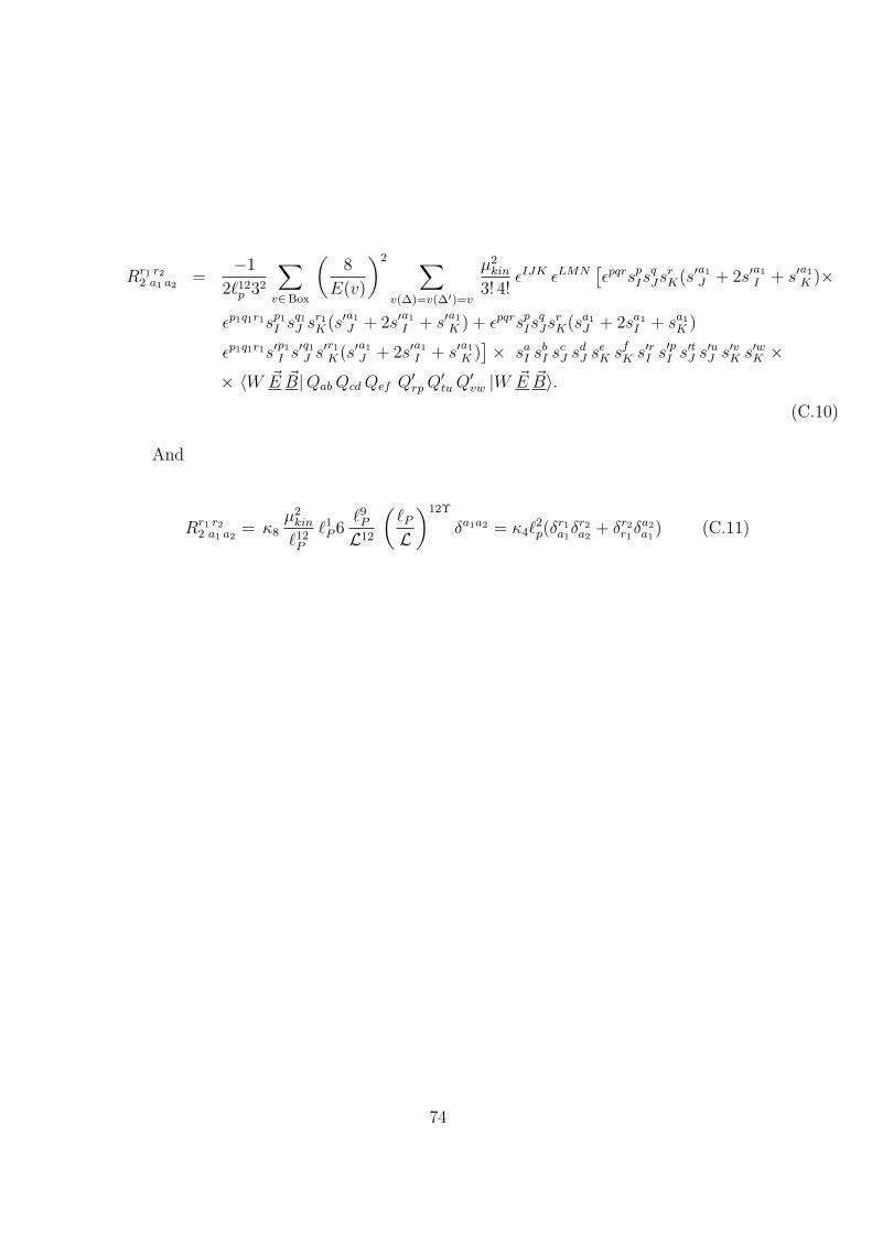
Rr1 r22 a1 a2
=−1
2`12p 32
∑v∈Box
(8
E(v)
)2 ∑
v(∆)=v(∆′)=v
µ2kin
3! 4!εIJK εLMN
[εpqrsp
IsqJsr
K(s′a1
J + 2s′a1
I + s′a1
K )×
εp1q1r1sp1
I sq1
J sr1K(s′a1
J + 2s′a1
I + s′a1
K ) + εpqrspIs
qJsr
K(sa1J + 2sa1
I + sa1K )
εp1q1r1s′p1
I s′q1
J s′r1
K(s′a1
J + 2s′a1
I + s′a1
K )]× sa
I sbI sc
J sdJ se
K sfK s′rI s′pI s′tJ s′uJ s′vK s′wK ×
× 〈W ~E ~B|Qab Qcd Qef Q′rp Q′
tu Q′vw |W ~E ~B〉.
(C.10)
And
Rr1 r22 a1 a2
= κ8µ2
kin
`12P
`1P 6
`9P
L12
(`P
L)12Υ
δa1a2 = κ4`2p(δ
r1a1
δr2a2
+ δr2r1
δa2a1
) (C.11)
74
Bibliography
[1] T. Jacobson and L. Smolin, “Nonperturbative Quantum Geometries,” Nucl.
Phys. B 299, 295 (1988).
[2] G. T. Horowitz, “Quantum gravity at the turn of the millennium,” arXiv:gr-
qc/0011089.
[3] S. Carlip, “Quantum gravity: A progress report,” Rept. Prog. Phys. 64, 885
(2001) [arXiv:gr-qc/0108040].
[4] C. Rovelli, “Loop quantum gravity,” Living Rev. Rel. 1, 1 (1998) [arXiv:gr-
qc/9710008].
[5] T. Thiemann, “Introduction to modern canonical quantum general relativity,”
arXiv:gr-qc/0110034.
[6] A. Ashtekar, “Lectures on nonperturbative canonical gravity,”
[7] J. Baez and J. P. Muniain, “Gauge fields, knots and gravity,”
[8] C. Kiefer, “Quantum gravity,”
[9] C. Rovelli, “Quantum gravity,”
[10] M. B. Green, J. H. Schwarz, E. Witten, Superstring Theory, Cambridge Uni-
versity Press (1988)
[11] J. Polchinski, String Theory, Cambridge University Press (1988)
[12] A. Connes, Non-commutative Geometry, Academic Press (1995)
75
[13] R Wald: Quantum field theory in curved spacetime and black hole thermodynam-
ics, Chicago University Press, 1994. Also: ND Birrel and PCW Davies: Quan-
tum fields in curved space, Cambridge University Press, 1982; and S Fulling:
Aspects of quantum field theory in curved space-time, Cambridge University
Press, 1989.
[14] R Sorkin gr-qc/9705006.
[15] DR Finkelstein, Quantum Relativity (Springer Berlin 1997)
[16] R Penrose, lecture at the GR15, Poona, India, December 1997.
[17] A Connes Noncommutative Geometry (Academic Press 1994). G Landi, An
introduction to Noncommutative Spaces and Their Geometries (Springer, Berlin
1998). J Madore An introduction to Noncommutative Differential Geometry
LMS Lecture Notes 206, 1995.
[18] S Frittelli, C Kozameh, ET Newman, J Math Phys 5 (1995) 4984, 5005, 6397.
[19] K. Eppley and E. Hannah, Found. Phys. 7, 51 (1977).
[20] B. S. Dewitt, “Quantum Theory Of Gravity. I. The Canonical Theory,” Phys.
Rev. 160 (1967) 1113.
B. S. Dewitt, “Quantum Theory Of Gravity. II. The Manifestly Covariant The-
ory,” Phys. Rev. 162 (1967) 1195.
B. S. Dewitt, “Quantum Theory Of Gravity. III. Applications Of The Covariant
Theory,” Phys. Rev. 162 (1967) 1239.
[21] L. Smolin, “Three roads to quantum gravity,”
[22] M. Gaul and C. Rovelli, “Loop quantum gravity and the meaning of diffeomor-
phism invariance,” Lect. Notes Phys. 541, 277 (2000) [arXiv:gr-qc/9910079].
[23] J. Glimm, A. Jaffe, “Quantum Physics”, Springer-Verlag, New York, 1987
[24] R. F. Streater and A. S. Wightman, “Pct, Spin And Statistics, And All That,”
76
[25] P. A. M. Dirac, “Lectures on Quantum Mechanics”, Belfer Graduate School of
Science, Yeshiva University Press, New York, 1964
[26] A. Hanson, T. Regge, C. Teitelboim, “Constrained Hamiltonian Systems”, Ac-
cdemia Nazionale dei Lincei, Roma, 1976
[27] D.M. Gitman, I. V. Tyutin, “Quantization of Fields with Constraints”,
Springer-Verlag, Berlin, 1990
[28] M. Henneaux, C. Teitelboim, “Quantization of Gauge Systems” Princeton Uni-
versity Press, Princeton, 1992
[29] A. Ashtekar, M. Stillerman, “Geometric Quantization and Constrained Sys-
tems”, Journ. Math. Phys. 27 (1986) 1319
[30] M. Gotay, “Constraints, Reduction and Quantization”, J.Math.Phys.27:2051-
2066,1986
[31] R. Arnowitt, S. Deser and C. W. Misner, “The Dynamics Of General Relativ-
ity,” arXiv:gr-qc/0405109.
[32] A. Ashtekar, Phys. Rev. Lett. 57, 2244 (1986); Phys. Rev. D36, 1587 (1987).
[33] C. Rovelli and L. Smolin, “Discreteness of area and volume in quantum gravity,”
Nucl. Phys. B 442, 593 (1995) [Erratum-ibid. B 456, 753 (1995)] [arXiv:gr-
qc/9411005].
[34] A. Ashtekar and J. Lewandowski, “Quantum theory of geometry. I: Area oper-
ators,” Class. Quant. Grav. 14, A55 (1997) [arXiv:gr-qc/9602046].
[35] A. Sen, Journ. Math. Phys. 22 (1981) 1781
A. Sen, Phys. Lett B119 (1982) 89
A. Sen, Int. Journ. Theor. Phys. 21 (1982) 1
[36] S. M. Carroll, “Lecture notes on general relativity,” arXiv:gr-qc/9712019.
[37] R. Gambini, J. Pullin, “Loops, Knots, Gauge Theories and Quantum Gravity”,
Cambridge University Press, Cambridge, 1996
77
[38] A. Ashtekar, J. Lewandowski, “Representation theory of analytic Holonomy C?
algebras”, in “Knots and Quantum Gravity”, J. Baez (ed.), Oxford University
Press, Oxford 1994
[39] R. Penrose, in : “Quantum Gravity and Beyond”, T. Bastin (ed.), Cambridge
University Press, Cambridge, 1971
[40] C. Rovelli, L. Smolin, “Spin Networks and Quantum Gravity”, Phys. Rev. D53
(1995) 5743
[41] J. Baez, “Spin Networks in Non-Perturbative Quantum Gravity”, in : “The
Interface of Knots and Physics”, L. Kauffman (ed.), American Mathematical
Society, Providence, Rhode Island, 1996, [gr-qc/9504036]
[42] C. Rovelli, L. Smolin, Nucl. Phys. B442 (1995) 593, Erratum : Nucl. Phys.
B456 (1995) 734
[43] R. Loll, “Spectrum of the Volume Operator in Quantum Gravity”,
Nucl.Phys.B460:143-154,1996 [gr-qc/9511030]
[44] R. Loll, Class. Quantum Grav. 14 (1997) 1725
R. Loll, Nucl. Phys. B500 (1997) 405
R. Loll, Phys. Rev. Lett. 75 (1995) 3048
[45] A. Ashtekar, J. Lewandowski, “Quantum Theory of Geometry I: Area Opera-
tors”, Class. Quantum Grav. 14 (1997) A55-81 A. Ashtekar, J. Lewandowski,
“Quantum Theory of Geometry II : Volume Operators”, Adv. Theo. Math.
Phys. 1 (1997) 388-429
J. Lewandowski, Class. Quantum Grav. 14 (1997) 71-76
[46] T. Thiemann, “A Length Operator for Canonical Quantum Gravity”, Journ.
Math. Phys. 39 (1998) 3372-3392, [gr-qc/9606092]
[47] P.A.M Dirac, Phys. Rev. 73 (1948) 1092
P.A.M Dirac, Rev. Mod. Phys. 21 (1949) 392
[48] H. A. Morales-Tecotl and C. Rovelli, “Fermions in quantum gravity,” Phys.
Rev. Lett. 72, 3642 (1994) [arXiv:gr-qc/9401011].
78
[49] H. A. Morales-Tecotl and C. Rovelli, “Loop space representation of quantum
fermions and gravity,” Nucl. Phys. B 451, 325 (1995).
[50] J. C. Baez and K. V. Krasnov, “Quantization of diffeomorphism-invariant the-
ories with fermions,” J. Math. Phys. 39, 1251 (1998) [arXiv:hep-th/9703112].
[51] T. Thiemann, “QSD V: Quantum gravity as the natural regulator of mat-
ter quantum field theories,” Class. Quant. Grav. 15, 1281 (1998) [arXiv:gr-
qc/9705019].
[52] T. Thiemann, “Quantum spin dynamics (QSD),” Class. Quant. Grav. 15, 839
(1998) [arXiv:gr-qc/9606089].
[53] J. Alfaro, H. A. Morales-Tecotl, M. Reyes and L. F. Urrutia, “On non-Abelian
holonomies,” J. Phys. A 36, 12097 (2003) [arXiv:hep-th/0304223].
[54] T. Thiemann, “Quantum Spin Dynamics (QSD) : VI. Quantum Poincare Al-
gebra and a Quantum Positivity of Energy Theorem for Canonical Quantum
Gravity”, Class. Quantum Grav. 15 (1998) 1463-1485, [gr-qc/9705020]
[55] T. Thiemann, “Quantum Spin Dynamics (QSD) : II. The Kernel of the Wheeler-
DeWitt Constraint Operator”, Class. Quantum Grav. 15 (1998) 875-905, [gr-
qc/9606090]
[56] J. Alfaro, H. A. Morales-Tecotl and L. F. Urrutia, “Quantum gravity correc-
tions to neutrino propagation,” Phys. Rev. Lett. 84, 2318 (2000) [arXiv:gr-
qc/9909079].
[57] J. Alfaro, H. A. Morales-Tecotl and L. F. Urrutia, “Loop quantum gravity and
light propagation,” Phys. Rev. D 65, 103509 (2002) [arXiv:hep-th/0108061].
[58] P. Fishbane, S. Gasiorowicz and P. Kaus, Phys. Rev. D24, 2324 (1981).
[59] See for example: N.E. Bralic, Phys. Rev. D22, 3090(1980); M. Hirayama and
S. Matsubara, Prog. Theor. Phys. 99, 691(1998); D. Diakonov and V. Petrov,
On the non-Abelian Stokes theorem, hep-lat/0008004; B. Broda, Non-Abelian
Stokes theorem in action, math-ph/0012035.
79
[60] J. Alfaro and G. Palma, Phys. Rev. D 65, 103516 (2002) [arXiv:hep-
th/0111176].
[61] J. Alfaro and G. Palma, “Loop quantum gravity and ultra high energy cosmic
rays,” Phys. Rev. D 67, 083003 (2003) [arXiv:hep-th/0208193].
[62] A. Ashtekar and C.J. Isham, Class. & Quan. Grav. 9, 1433 (1992).
[63] A. Ashtekar and J. Lewandowski, “Representation theory of analytic holonomy
C? algebras”, in Knots and quantum gravity, J. Baez (ed), (Oxford University
Press, Oxford 1994).
[64] A. Ashtekar and J. Lewandowski, “Differential geometry on the space of con-
nections via graphs and projective limits”, Journ. Geo. Physics 17 (1995) 191
[65] A. Ashtekar and J. Lewandowski, J. Math. Phys. 36, 2170 (1995).
[66] D. Marolf and J. M. Mourao, “On the support of the Ashtekar-Lewandowski
measure”, Commun. Math. Phys. 170 (1995) 583-606
[67] A. Ashtekar, J. Lewandowski, D. Marolf, J. Mourao, T. Thiemann, “Quantiza-
tion for diffeomorphism invariant theories of connections with local degrees of
freedom”, Journ. Math. Phys. 36 (1995) 519-551
[68] J. Alfaro, M. Reyes, H. A. Morales-Tecotl and L. F. Urrutia, “On alterna-
tive approaches to Lorentz violation in loop quantum gravity inspired models,”
arXiv:gr-qc/0404113.
[69] A. Ashtekar, C. Rovelli, L. Smolin, “Weaving a Classical Geometry with Quan-
tum Threads”, Phys.Rev.Lett.69:237-240,1992, [hep-th/9203079]
J. Zegwaard, “Weaving of Curved Geometries”, Phys.Lett.B300:217-222,1993,
[hep-th/9210033]
J. Zegwaard, “Gravitons in Loop Quantum Gravity”, Nucl.Phys.B378:288-
308,1992
J. Iwasaki, C. Rovelli, “Gravitons as Embroidery of the Weave”,
Int.J.Mod.Phys.D1:533-557,1993
J. Iwasaki, C. Rovelli, “Gravitons from Loops: Nonperturbative Loop
80
Space Quantum Gravity Contains The Graviton Physics Approximation”,
Class.Quant.Grav.11:1653-1676,1994
Y. Ma, Y. Ling, “The Classical Geometry from a Physical State in Canonical
Qunatum Gravity”, Phys.Rev.D62:064030,2000, [gr-qc/0004070]
[70] M. Arnsdorf, Sameer Gupta, “Loop Quantum Gravity on Noncompact Spaces”,
Nucl.Phys.B577:529-546,2000, [gr-qc/9909053]
M. Arnsdorf, “Approximating Connections in Loop Quantum Gravity”, gr-
qc/9910084
[71] M. Varadarajan, J. A. Zapata, “A proposal for Analyzing the Classical
Limit of Kinematic Loop Gravity”, Class.Quant.Grav.17:4085-4110,2000, [gr-
qc/0001040]
[72] L. Bombelli, “Statistical Lorentzian Geometry and the Closeness of Lorentzian
Manifolds, J.Math.Phys.41:6944-6958,2000, [gr-qc/0002053]
[73] T. Thiemann, “Quantum Spin Dynamics (QSD): VII. Symplectic Structures
and Continuum Lattice Formulations of Gauge Field Theories”, T. Thiemann,
Class.Quant.Grav.18:3293-3338,2001, [hep-th/0005232]
T. Thiemann, “Gauge Field Theory Coherent States (GCS): I. General Prop-
erties”, Class.Quant.Grav.18:2025-2064,2001, [hep-th/0005233]
[74] T. Thiemann, O. Winkler, “Gauge Field Theory Coherent States
(GCS): II. Peakedness Properties”, Class.Quant.Grav.18:2561-2636,2001, [hep-
th/0005237]
T. Thiemann, O. Winkler, “Gauge Field Theory Coherent States (GCS): III.
Ehrenfest Theorems”, accepted for publ. by Class. Quantum Grav., [hep-
th/0005234]
[75] T. Thiemann, O. Winkler, “Gauge Field Theory Coherent States (GCS): IV.
Infinite Tensor Product and Thermodynamical Limit”, accepted for publ. by
Class. Quantum Grav., hep-th/0005235
81
[76] H. Sahlmann, T. Thiemann, O. Winkler, “ Coherent States for Canoni-
cal Quantum General Relativity and the Infinite Tensor product Extension”,
Nucl.Phys.B606:401-440,2001, [gr-qc/0102038]
[77] M. Varadarajan, “Fock representations from U(1) Holonomy Algebras”,
Phys.Rev.D61:104001,2000, [gr-qc/0001050]
M. Varadarajan, “Photons from Quantized Electric Flux Representations”, gr-
qc/0104051
M. Varadarajan, “Photons from Quantized Electric Flux Representations”, in
preparation
[78] A. Ashtekar, C. Rovelli and L. Smolin, “Weaving A Classical Geometry With
Quantum Threads,” Phys. Rev. Lett. 69, 237 (1992) [arXiv:hep-th/9203079].
[79] P. G. Bergmann and A. B. Komar, “Modified Supersymmetries,” Int. J. Theor.
Phys. 17, 377 (1978).
[80] G. T. Horowitz and R. C. Myers, “The value of singularities,” Gen. Rel. Grav.
27, 915 (1995) [arXiv:gr-qc/9503062].
[81] G. Horowitz, talk given at the 9th Marcel Grossmann Meeting, Rome, Italy
(2000), to appear in the Proceedings, eds. V. G. Gurzadyan, R. Jantzen, R.
Ruffini, Singapore, World Scientific, gr-qc/0011089
[82] C. Rovelli, lecture given at the GR15 conference, Pune, India (1998), gr-
qc/9803024
[83] S. Carlip, Rep. Prog. Phys. 64, 8, 885 (2001), gr-qc/
[84] Quantum structure of space and time M.J.Duff and C.J.Isham.
[85] T. Thiemann, “Kinematical Hilbert spaces for fermionic and Higgs quantum
field theories,” Class. Quant. Grav. 15, 1487 (1998) [arXiv:gr-qc/9705021].
82
Recommended