LOGO
Analysis of Unemployment
Qi Li Trung Le
David PetitBrian Weinberg
Dwaraka PolakamDoug Skipper-Dotta
Team #4
Team #4
Table of Contents
Concepts of Unemployment1
Descriptive Data Analysis2
Statistical Analysis3
Conclusions 4
Questions?5
Group #4
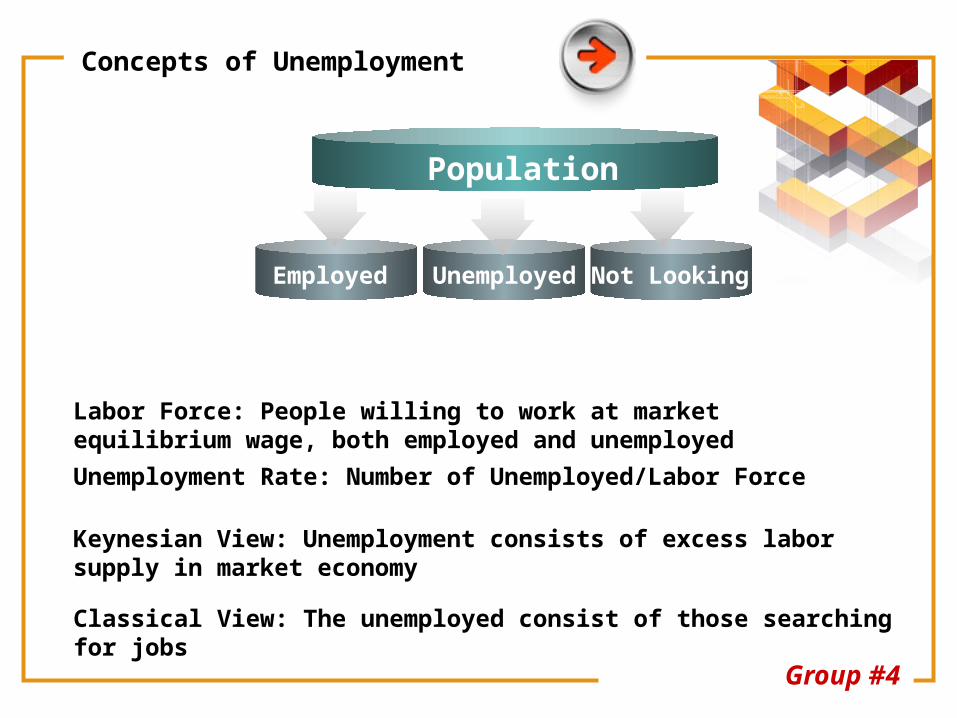
Concepts of Unemployment
Employed Unemployed Not Looking
Population
Labor ForceLabor Force: People willing to work at market equilibrium wage, both employed and unemployed
Unemployment Rate: Number of Unemployed/Labor Force
Keynesian View: Unemployment consists of excess labor supply in market economy
Classical View: The unemployed consist of those searching for jobs
Team #4
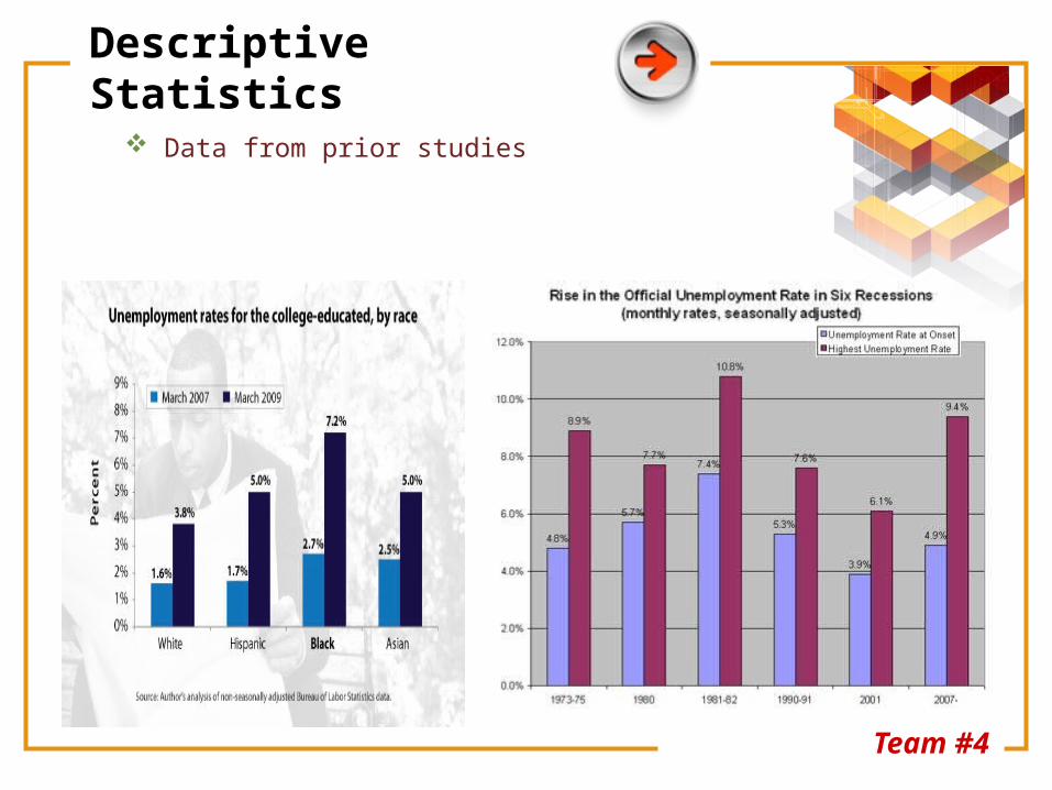
Descriptive Statistics
Data from prior studies
Variables
Unemployment Rate No Degree/Degree Men/Women White/Minority
Other Rates Crime Rate Suicide Rate Welfare Budget Annual Income Per Capita
Team #4
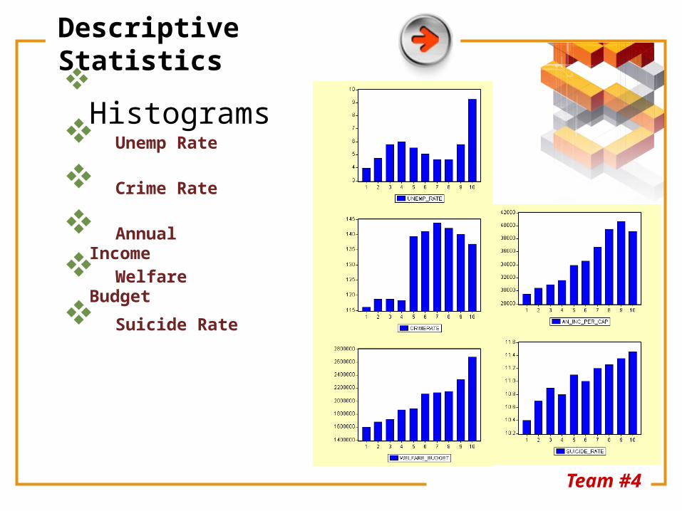
Descriptive Statistics Histograms
Crime Rate
Annual Income
Suicide Rate
Welfare Budget
Unemp Rate
Team #4
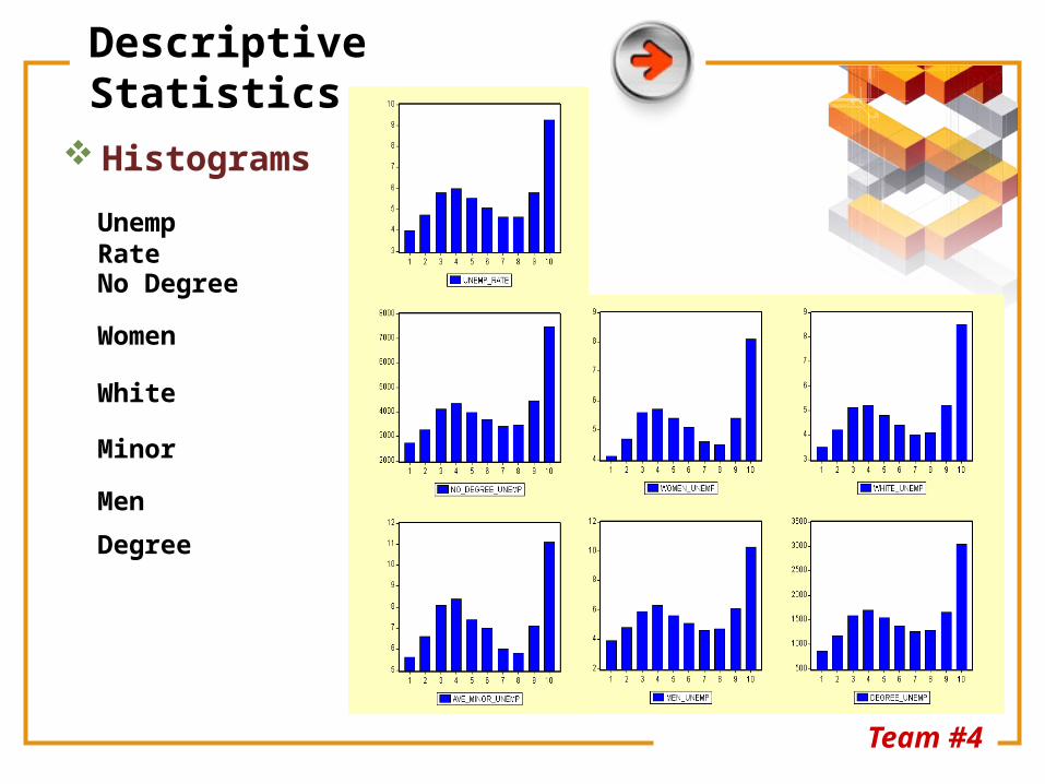
Descriptive Statistics
Histograms
No Degree
Women
White
Minor
Unemp Rate
Men
Degree
Exploratory Data Analysis
Team #4
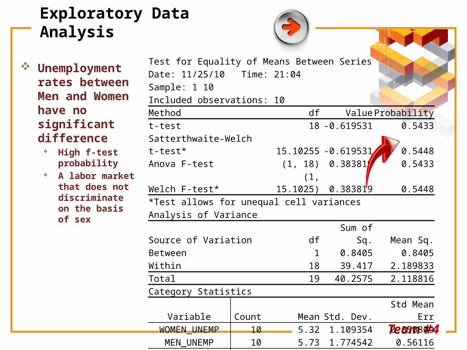
Test for Equality of Means Between SeriesDate: 11/25/10 Time: 21:04Sample: 1 10Included observations: 10 Method df Value Probabilityt-test 18 -0.619531 0.5433Satterthwaite-Welch t-test* 15.10255 -0.619531 0.5448Anova F-test (1, 18) 0.383819 0.5433Welch F-test* (1, 15.1025) 0.383819 0.5448*Test allows for unequal cell variances Analysis of Variance Source of Variation df Sum of Sq. Mean Sq.Between 1 0.8405 0.8405Within 18 39.417 2.189833Total 19 40.2575 2.118816Category Statistics
Variable Count Mean Std. Dev. Std Mean ErrWOMEN_UNEMP 10 5.32 1.109354 0.350809
MEN_UNEMP 10 5.73 1.774542 0.56116All 20 5.525 1.455615 0.325485
Unemployment rates between Men and Women have no significant difference
High f-test probability
A labor market that does not discriminate on the basis of sex
Team #4
Exploratory Data Analysis
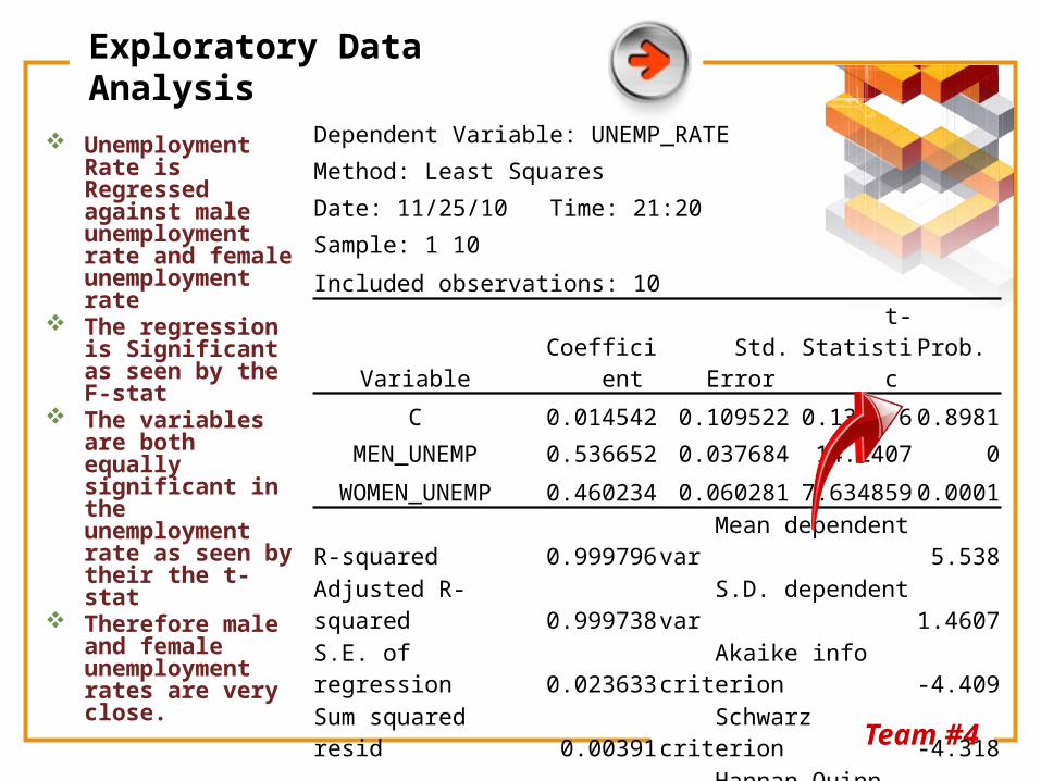
Unemployment Rate is Regressed against male unemployment rate and female unemployment rate
The regression is Significant as seen by the F-stat
The variables are both equally significant in the unemployment rate as seen by their the t-stat
Therefore male and female unemployment rates are very close.
Dependent Variable: UNEMP_RATE
Method: Least Squares
Date: 11/25/10 Time: 21:20
Sample: 1 10
Included observations: 10
Variable Coefficient Std. Error t-Statistic Prob.
C 0.014542 0.109522 0.132776 0.8981
MEN_UNEMP 0.536652 0.037684 14.2407 0
WOMEN_UNEMP 0.460234 0.060281 7.634859 0.0001
R-squared 0.999796 Mean dependent var 5.538
Adjusted R-squared 0.999738 S.D. dependent var 1.4607
S.E. of regression 0.023633 Akaike info criterion -4.409
Sum squared resid 0.00391 Schwarz criterion -4.318
Log likelihood 25.04513 Hannan-Quinn criter. -4.5086
F-statistic 17187.56 Durbin-Watson stat 3.3868
Prob(F-statistic) 0
Team #4
Exploratory Data Analysis
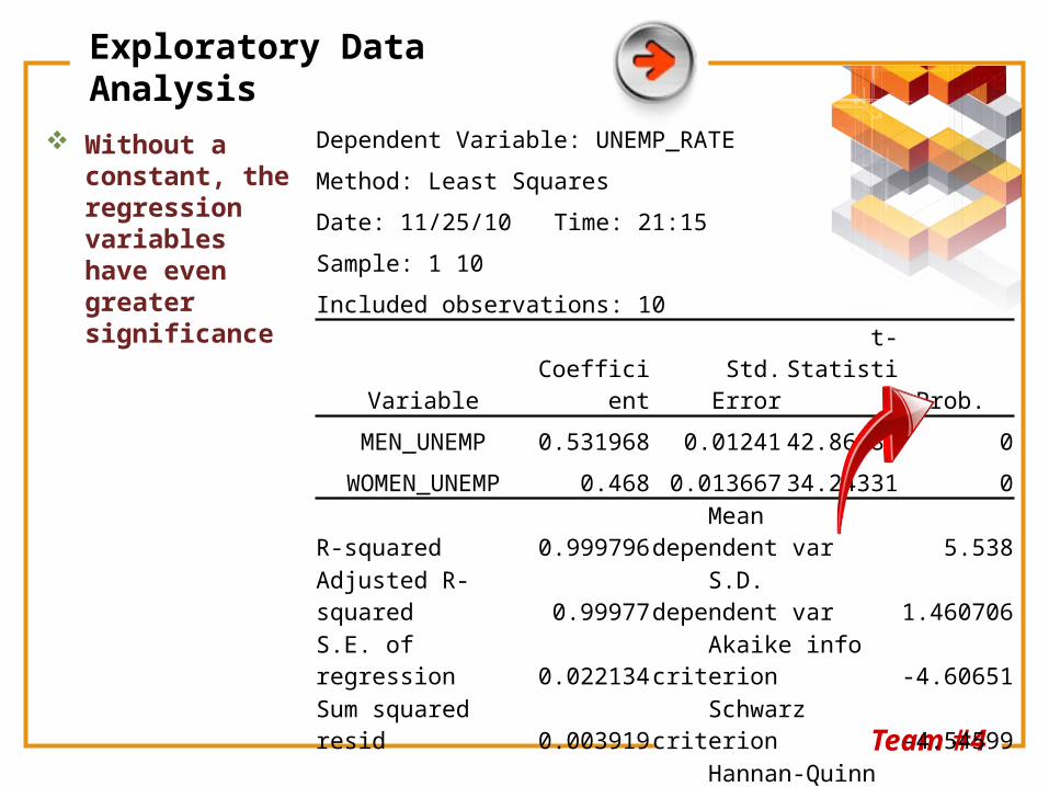
Without a constant, the regression variables have even greater significance
Dependent Variable: UNEMP_RATE
Method: Least Squares
Date: 11/25/10 Time: 21:15
Sample: 1 10
Included observations: 10
Variable Coefficient Std. Error t-Statistic Prob.
MEN_UNEMP 0.531968 0.01241 42.86486 0
WOMEN_UNEMP 0.468 0.013667 34.24331 0
R-squared 0.999796 Mean dependent var 5.538
Adjusted R-squared 0.99977 S.D. dependent var 1.460706
S.E. of regression 0.022134 Akaike info criterion -4.60651
Sum squared resid 0.003919 Schwarz criterion -4.54599
Log likelihood 25.03255 Hannan-Quinn criter. -4.6729
Durbin-Watson stat 3.327676
Team #4
Exploratory Data Analysis
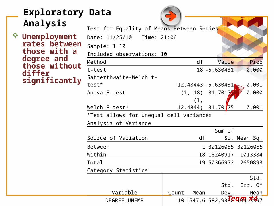
Unemployment rates between those with a degree and those without differ significantly
Test for Equality of Means Between Series
Date: 11/25/10 Time: 21:06
Sample: 1 10
Included observations: 10
Method df Value Prob
t-test 18 -5.630431 0.000
Satterthwaite-Welch t-test* 12.48443 -5.630431 0.001
Anova F-test (1, 18) 31.70175 0.000
Welch F-test* (1, 12.4844) 31.70175 0.001
*Test allows for unequal cell variances
Analysis of Variance
Source of Variation df Sum of Sq. Mean Sq.
Between 1 32126055 32126055
Within 18 18240917 1013384
Total 19 50366972 2650893
Category Statistics
Variable Count Mean Std. Dev.Std. Err. Of
Mean
DEGREE_UNEMP 10 1547.6 582.9332 184.3397
NO_DEGREE_UNEMP 10 4082.4 1298.829 410.7259
All 20 2815 1628.156 364.0668
Team #4
Exploratory Data Analysis
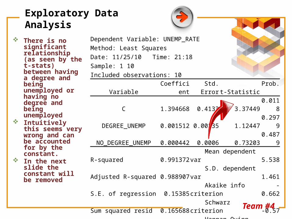
There is no significant relationship (as seen by the t-stats) between having a degree and being unemployed or having no degree and being unemployed
Intuitively this seems very wrong and can be accounted for by the constant.
In the next slide the constant will be removed
Dependent Variable: UNEMP_RATE
Method: Least Squares
Date: 11/25/10 Time: 21:18
Sample: 1 10
Included observations: 10
Variable Coefficient Std. Error t-Statistic Prob.
C 1.394668 0.4133 3.37449 0.0118
DEGREE_UNEMP 0.001512 0.00135 1.12447 0.2979
NO_DEGREE_UNEMP 0.000442 0.0006 0.73203 0.4879
R-squared 0.991372 Mean dependent var 5.538
Adjusted R-squared 0.988907 S.D. dependent var 1.461
S.E. of regression 0.15385 Akaike info criterion -0.662
Sum squared resid 0.165688 Schwarz criterion -0.57
Log likelihood 6.311784 Hannan-Quinn criter. -0.762
F-statistic 402.1441 Durbin-Watson stat 0.437
Prob(F-statistic) 0
Team #4
Exploratory Data Analysis
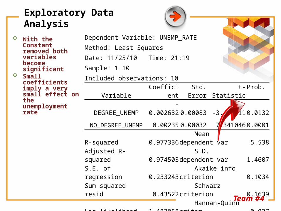
With the Constant removed both variables become significant
Small coefficients imply a very small effect on the unemployment rate
Dependent Variable: UNEMP_RATE
Method: Least Squares
Date: 11/25/10 Time: 21:19
Sample: 1 10
Included observations: 10
Variable Coefficient Std. Error t-Statistic Prob.
DEGREE_UNEMP -0.002632 0.00083 -3.169111 0.0132
NO_DEGREE_UNEMP 0.00235 0.00032 7.341046 0.0001
R-squared 0.977336 Mean dependent var 5.538
Adjusted R-squared 0.974503 S.D. dependent var 1.4607
S.E. of regression 0.233243 Akaike info criterion 0.1034
Sum squared resid 0.43522 Schwarz criterion 0.1639
Log likelihood 1.483058 Hannan-Quinn criter. 0.037
Durbin-Watson stat 0.492591
Team #4
Exploratory Data Analysis
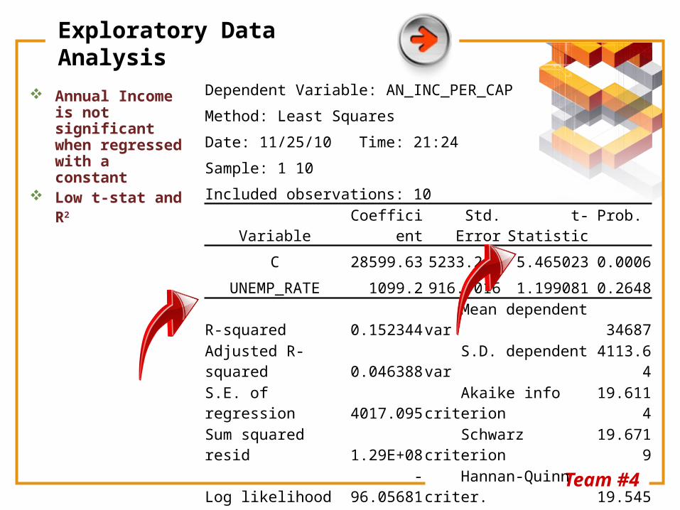
Annual Income is not significant when regressed with a constant
Low t-stat and R2
Dependent Variable: AN_INC_PER_CAP
Method: Least Squares
Date: 11/25/10 Time: 21:24
Sample: 1 10
Included observations: 10
Variable Coefficient Std. Error t-Statistic Prob.
C 28599.63 5233.213 5.465023 0.0006
UNEMP_RATE 1099.2 916.7016 1.199081 0.2648
R-squared 0.152344 Mean dependent var 34687
Adjusted R-squared 0.046388 S.D. dependent var 4113.64
S.E. of regression 4017.095 Akaike info criterion 19.6114
Sum squared resid 1.29E+08 Schwarz criterion 19.6719
Log likelihood -96.05681 Hannan-Quinn criter. 19.545
F-statistic 1.437796 Durbin-Watson stat 0.41066
Prob(F-statistic) 0.264805
Team #4
Exploratory Data Analysis
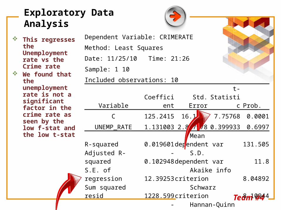
This regresses the Unemployment rate vs the Crime rate
We found that the unemployment rate is not a significant factor in the crime rate as seen by the low f-stat and the low t-stat
Dependent Variable: CRIMERATE
Method: Least Squares
Date: 11/25/10 Time: 21:26
Sample: 1 10
Included observations: 10
Variable Coefficient Std. Error t-Statistic Prob.
C 125.2415 16.1442 7.75768 0.0001
UNEMP_RATE 1.131003 2.827978 0.399933 0.6997
R-squared 0.019601 Mean dependent var 131.505
Adjusted R-squared -0.102948 S.D. dependent var 11.8
S.E. of regression 12.39253 Akaike info criterion 8.04892
Sum squared resid 1228.599 Schwarz criterion 8.10944
Log likelihood -38.24461 Hannan-Quinn criter. 7.98254
F-statistic 0.159947 Durbin-Watson stat 0.45088
Prob(F-statistic) 0.699672
Team #4
Exploratory Data Analysis
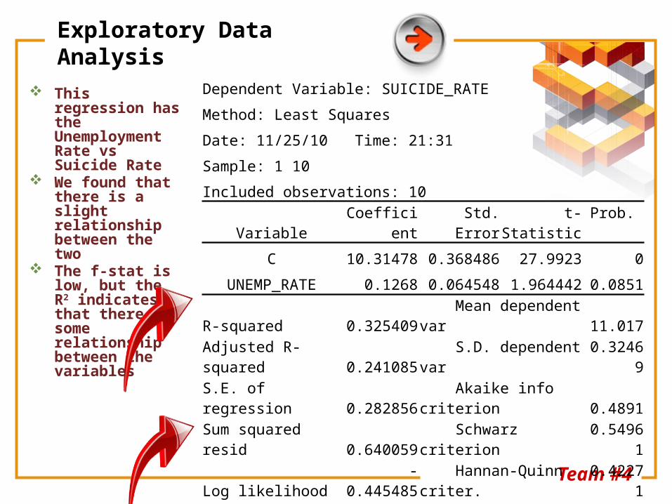
This regression has the Unemployment Rate vs Suicide Rate
We found that there is a slight relationship between the two
The f-stat is low, but the R2 indicates that there is some relationship between the variables
Dependent Variable: SUICIDE_RATE
Method: Least Squares
Date: 11/25/10 Time: 21:31
Sample: 1 10
Included observations: 10
Variable Coefficient Std. Error t-Statistic Prob.
C 10.31478 0.368486 27.9923 0
UNEMP_RATE 0.1268 0.064548 1.964442 0.0851
R-squared 0.325409 Mean dependent var 11.017
Adjusted R-squared 0.241085 S.D. dependent var 0.32469
S.E. of regression 0.282856 Akaike info criterion 0.4891
Sum squared resid 0.640059 Schwarz criterion 0.54961
Log likelihood -0.445485 Hannan-Quinn criter. 0.42271
F-statistic 3.859031 Durbin-Watson stat 0.58848
Prob(F-statistic) 0.085072
Team #4
Exploratory Data Analysis
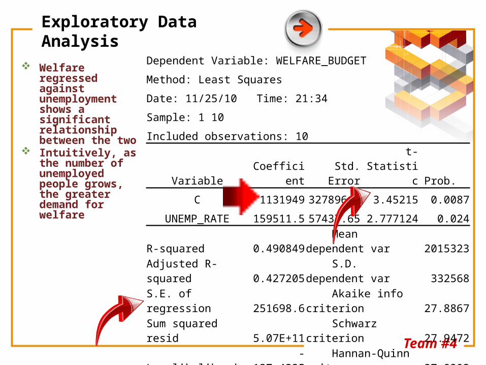
Welfare regressed against unemployment shows a significant relationship between the two
Intuitively, as the number of unemployed people grows, the greater demand for welfare
Dependent Variable: WELFARE_BUDGET
Method: Least Squares
Date: 11/25/10 Time: 21:34
Sample: 1 10
Included observations: 10
Variable Coefficient Std. Error t-Statistic Prob.
C 1131949 327896.7 3.45215 0.0087
UNEMP_RATE 159511.5 57437.65 2.777124 0.024
R-squared 0.490849 Mean dependent var 2015323
Adjusted R-squared 0.427205 S.D. dependent var 332568
S.E. of regression 251698.6 Akaike info criterion 27.8867
Sum squared resid 5.07E+11 Schwarz criterion 27.9472
Log likelihood -137.4335 Hannan-Quinn criter. 27.8203
F-statistic 7.712418 Durbin-Watson stat 0.35586
Prob(F-statistic) 0.024031

Team #4
Exploratory Data Analysis
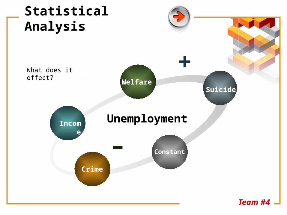
Here the Unemployment Rate is regressed against multiple variables
All variables are significantly contribute to the Unemployment Rate
Annual Inc per cap coefficient is negative, suggesting a higher income implies a lower unemployment rate
Surprisingly, as crime rate increases unemployment decreases
Dependent Variable: UNEMP_RATE
Method: Least Squares
Date: 11/28/10 Time: 12:20
Sample: 1 10
Included observations: 10
Variable Coefficient Std. Error t-Statistic Prob.
AN_INC_PER_CAP -0.000411 0.000113 -3.64743 0.0148
CRIMERATE -0.083554 0.02457 -3.40071 0.0192
SUICIDE_RATE 4.728742 1.383211 3.418669 0.0189
WELFARE_BUDGET 5.61E-06 1.13E-06 4.979503 0.0042
C -32.63094 11.73778 -2.77999 0.0389
R-squared 0.948687 Mean dependent var 5.538
Adjusted R-squared 0.907637 S.D. dependent var 1.46071
S.E. of regression 0.443928 Akaike info criterion 1.52054
Sum squared resid 0.98536 Schwarz criterion 1.67184
Log likelihood -2.602719 F-statistic 23.1103
Durbin-Watson stat 2.027352 Prob(F-statistic) 0.00201
Team #4
Statistical Analysis
Income
WelfareSuicide
Constant
Crime
Unemployment
What does it effect?
–
+
Team #4
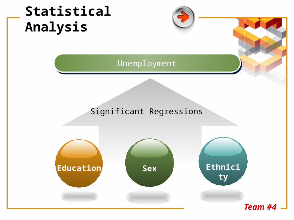
Statistical Analysis
UnemploymentUnemployment
Significant Regressions
Education Sex Ethnicity
Team #4
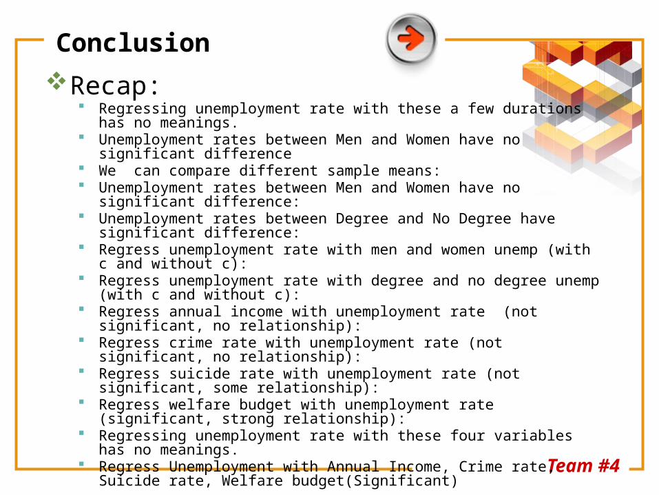
Conclusion
Recap: Regressing unemployment rate with these a few durations has no meanings. Unemployment rates between Men and Women have no significant difference We can compare different sample means: Unemployment rates between Men and Women have no significant
difference: Unemployment rates between Degree and No Degree have significant
difference: Regress unemployment rate with men and women unemp (with c and without
c): Regress unemployment rate with degree and no degree unemp (with c and
without c): Regress annual income with unemployment rate (not significant, no
relationship): Regress crime rate with unemployment rate (not significant, no relationship): Regress suicide rate with unemployment rate (not significant, some
relationship): Regress welfare budget with unemployment rate (significant, strong
relationship): Regressing unemployment rate with these four variables has no meanings. Regress Unemployment with Annual Income, Crime rate, Suicide rate,
Welfare budget(Significant)
Team #4
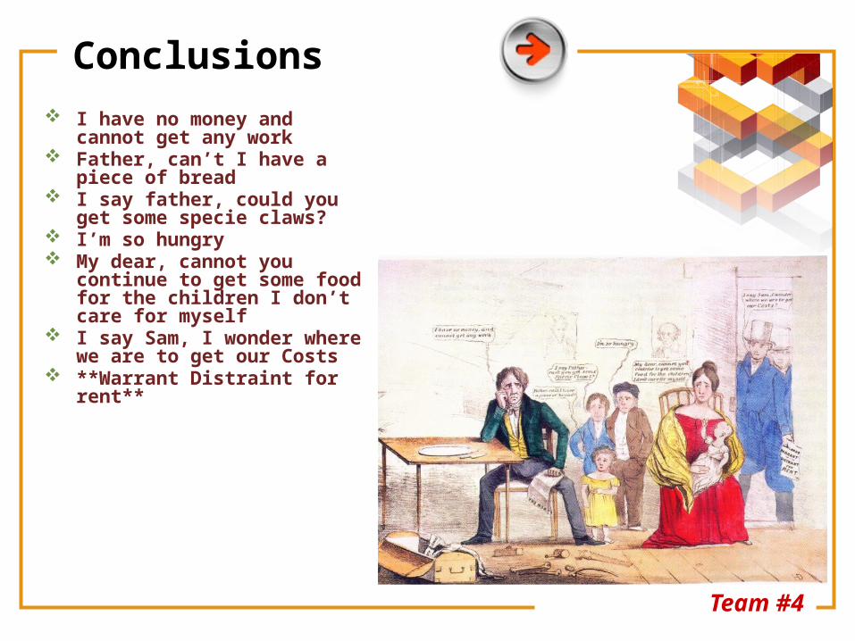
Conclusions I have no money and cannot
get any work Father, can’t I have a piece of
bread I say father, could you get
some specie claws? I’m so hungry My dear, cannot you continue
to get some food for the children I don’t care for myself
I say Sam, I wonder where we are to get our Costs
**Warrant Distraint for rent**
Team #4
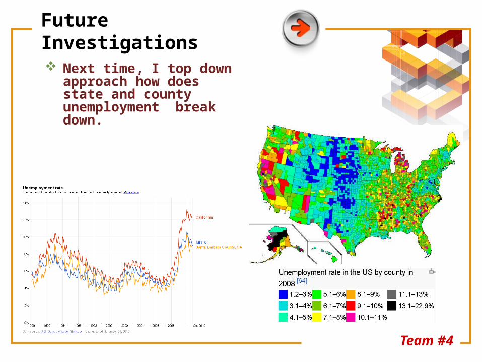
Future Investigations
Next time, I top down approach how does state and county unemployment break down.
Team #4
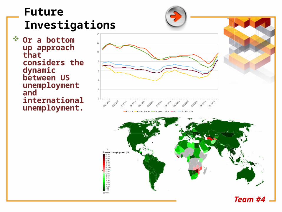
Future Investigations
Or a bottom up approach that considers the dynamic between US unemployment and international unemployment.

LOGO
Team #4
Team #4
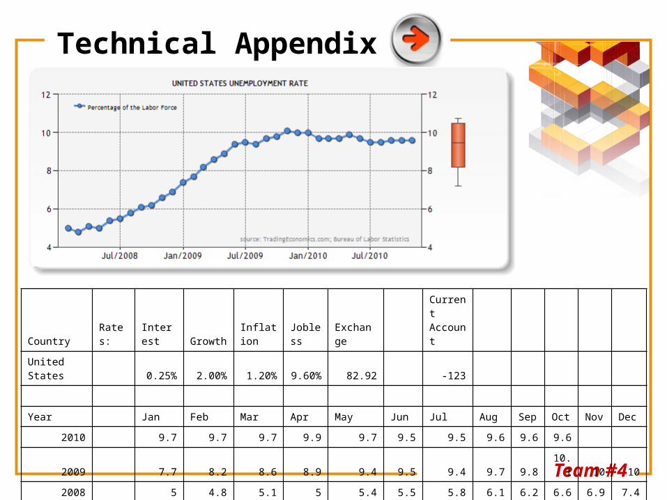
Technical Appendix
Country Rates: Interest Growth Inflation Jobless Exchange Current Account
United States 0.25% 2.00% 1.20% 9.60% 82.92 -123
Year Jan Feb Mar Apr May Jun Jul Aug Sep Oct Nov Dec
2010 9.7 9.7 9.7 9.9 9.7 9.5 9.5 9.6 9.6 9.6
2009 7.7 8.2 8.6 8.9 9.4 9.5 9.4 9.7 9.8 10.1 10 10
2008 5 4.8 5.1 5 5.4 5.5 5.8 6.1 6.2 6.6 6.9 7.4
Team #4
Works Cited http://www.bls.gov/cps/ http://en.wikipedia.org/wiki/
Unemployment http:://en.wikipedia.org/wiki/
File:Panic1873.jpg http://upload.wikimedia.org/
wikipedia/commons/c/ce/Chomage-oecd-t3-2009.png
Recommended