SF - M2 SAR - 2014/2015
Logique temporelle et Model-Checking
Nathalie Sznajder Université Pierre et Marie Curie, LIP6

SF - M2 SAR - 2014/2015
Les méthodes formelles
• Preuve assistée par ordinateur
• Test
• Model-Checking
SF - M2 SAR - 2014/2015
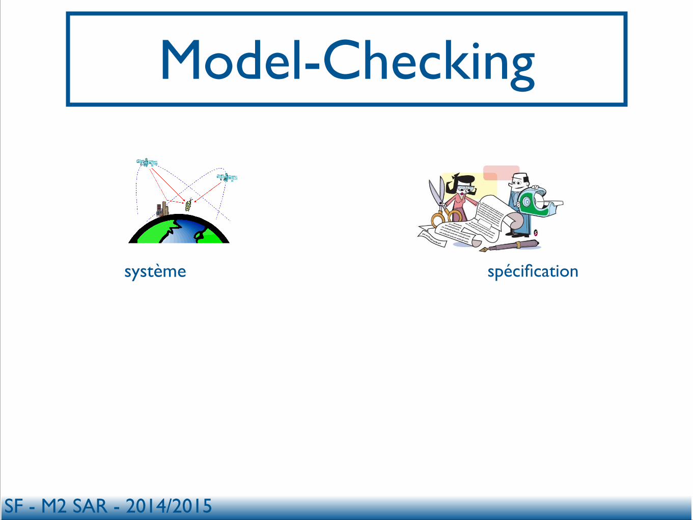
Model-CheckingIntroduction
Principles of model checking
Does
system
satisfy
specification
?
model
'
formula
?|=model-checker
Nathalie Bertrand Model checking VTS – M2RI – 2011 3/86
système
Introduction
Principles of model checking
Does
system
satisfy
specification
?
model
'
formula
?|=model-checker
Nathalie Bertrand Model checking VTS – M2RI – 2011 3/86
spécification

SF - M2 SAR - 2014/2015
Est-ce que le
Model-CheckingIntroduction
Principles of model checking
Does
system
satisfy
specification
?
model
'
formula
?|=model-checker
Nathalie Bertrand Model checking VTS – M2RI – 2011 3/86
système
Introduction
Principles of model checking
Does
system
satisfy
specification
?
model
'
formula
?|=model-checker
Nathalie Bertrand Model checking VTS – M2RI – 2011 3/86
spécification
satisfait ?

SF - M2 SAR - 2014/2015
Est-ce que le
Model-Checking
Figure 1: essai
blablabla
1
Introduction
Principles of model checking
Does
system
satisfy
specification
?
model
'
formula
?|=model-checker
Nathalie Bertrand Model checking VTS – M2RI – 2011 3/86
système
Introduction
Principles of model checking
Does
system
satisfy
specification
?
model
'
formula
?|=model-checker
Nathalie Bertrand Model checking VTS – M2RI – 2011 3/86
spécification
satisfait ?
modèle
Introduction
Principles of model checking
Does
system
satisfy
specification
?
model
'
formula
?|=model-checker
Nathalie Bertrand Model checking VTS – M2RI – 2011 3/86

SF - M2 SAR - 2014/2015
Est-ce que le
Model-Checking
Figure 1: essai
blablabla
1
Introduction
Principles of model checking
Does
system
satisfy
specification
?
model
'
formula
?|=model-checker
Nathalie Bertrand Model checking VTS – M2RI – 2011 3/86
système
Introduction
Principles of model checking
Does
system
satisfy
specification
?
model
'
formula
?|=model-checker
Nathalie Bertrand Model checking VTS – M2RI – 2011 3/86
spécification
satisfait ?
modèle
Figure 1: essai
blablabla'
1
formule
Introduction
Principles of model checking
Does
system
satisfy
specification
?
model
'
formula
?|=model-checker
Nathalie Bertrand Model checking VTS – M2RI – 2011 3/86
Introduction
Principles of model checking
Does
system
satisfy
specification
?
model
'
formula
?|=model-checker
Nathalie Bertrand Model checking VTS – M2RI – 2011 3/86

SF - M2 SAR - 2014/2015
Est-ce que le
Model-Checking
Figure 1: essai
blablabla
1
Introduction
Principles of model checking
Does
system
satisfy
specification
?
model
'
formula
?|=model-checker
Nathalie Bertrand Model checking VTS – M2RI – 2011 3/86
système
Introduction
Principles of model checking
Does
system
satisfy
specification
?
model
'
formula
?|=model-checker
Nathalie Bertrand Model checking VTS – M2RI – 2011 3/86
spécification
satisfait ?
modèle
Figure 1: essai
blablabla'
1
formule
⊧ ?algorithme de Model Checking
Introduction
Principles of model checking
Does
system
satisfy
specification
?
model
'
formula
?|=model-checker
Nathalie Bertrand Model checking VTS – M2RI – 2011 3/86
Introduction
Principles of model checking
Does
system
satisfy
specification
?
model
'
formula
?|=model-checker
Nathalie Bertrand Model checking VTS – M2RI – 2011 3/86
Introduction
Principles of model checking
Does
system
satisfy
specification
?
model
'
formula
?|=model-checker
Nathalie Bertrand Model checking VTS – M2RI – 2011 3/86

SF - M2 SAR - 2014/2015
Références bibliographiques
• Model Checking, E. Clarke, O. Grumberg, D. Peled, MIT Press 99
• Vérification de logiciels : techniques et outils du model-checking, P. Schnoebelen, B. Bérard, M. Bidoit, F. Laroussinie, A. Petit, Vuibert 99
• Principles of Model-Checking, C. Baier, J.-P. Katoen, MIT Press 08

SF - M2 SAR - 2014/2015
Plan
1. Modélisation
2. Spécifications
1. Généralités sur les spécifications
2. LTL
3. CTL
3. Algorithmes de Model-Checking
1. LTL
2. CTL
3. Inclure des notions d’équité

SF - M2 SAR - 2014/2015
1. Modélisation• On veut vérifier comportement du système au
cours du temps.
• Notion d’état à un instant donné
• Actions du système →changement d’état.
• →Système de transition
• Informations supplémentaires sur
• communication (notion d’action)
• propriétés vérifiées par les états (propositions atomiques)

SF - M2 SAR - 2014/2015
Structure de Kripke• Définition: M=(Q,T, A, q0, AP, l)
• Q : ensemble fini d’états
• A : alphabet d’actions (facultatif)
• T : relation de transitions entre états
• q0 : état initial
• AP : ensemble de propositions atomiques
• l : Q 2AP, étiquetage des états

SF - M2 SAR - 2014/2015
• Soit M=(Q,T, A, q0, AP, l) une structure de Kripke.
• Soit q un état. L’ensemble {q’∈Q| il existe a ∈A, (q,a,q’)∈T} est l’ensemble des successeurs de q.
Structure de Kripke

SF - M2 SAR - 2014/2015
Exemple: distributeur
Transition Systems 21
the likelihood with which a certain transition is selected. Similarly, when the set of initialstates consists of more than one state, the start state is selected nondeterministically.
The labeling function L relates a set L(s) ∈ 2AP of atomic propositions to any state s.1
L(s) intuitively stands for exactly those atomic propositions a ∈ AP which are satisfiedby state s. Given that Φ is a propositional logic formula, then s satisfies the formula Φ ifthe evaluation induced by L(s) makes the formula Φ true; that is:
s |= Φ iff L(s) |= Φ.
(Basic principles of propositional logic are explained in Appendix A.3, see page 915 ff.)
Example 2.2. Beverage Vending Machine
We consider an (somewhat foolish) example, which has been established as standard in thefield of process calculi. The transition system in Figure 2.1 models a preliminary designof a beverage vending machine. The machine can either deliver beer or soda. States arerepresented by ovals and transitions by labeled edges. State names are depicted inside theovals. Initial states are indicated by having an incoming arrow without source.
pay
selectsoda beer
insert coin
ττ
get soda get beer
Figure 2.1: A transition system of a simple beverage vending machine.
The state space is S = { pay , select , soda , beer }. The set of initial states consists ofonly one state, i.e., I = { pay }. The (user) action insert coin denotes the insertion of acoin, while the (machine) actions get soda and get beer denote the delivery of soda andbeer, respectively. Transitions of which the action label is not of further interest here,e.g., as it denotes some internal activity of the beverage machine, are all denoted by thedistinguished action symbol τ . We have:
Act = { insert coin , get soda , get beer , τ }.
Some example transitions are:
pay insert coin−−−−−−−−→ select and beer get beer−−−−−−→ pay .
1Recall that 2AP denotes the power set of AP.
[Principles of Model-Checking, C. Baier, J.-P. Katoen]
{paid, drink} {paid, drink}
{paid}

SF - M2 SAR - 2014/2015
Exemple: circuitTransition Systems 27
XOR
OR
yNOT
x
r x r y
x 0 r 0
x 0 r 1
x 1 r 0
x 1 r 1r
x y
Figure 2.2: Transition system representation of a simple hardware circuit.
where ⊕ stands for exclusive or (XOR, or parity function). The register evaluation changesaccording to the circuit function
δr = x ∨ r .
Note that once the register evaluation is [r = 1], r keeps that value. Under the initialregister evaluation [r = 0], the circuit behavior is modeled by the transition system TSwith state space
S = Eval(x, r)
where Eval(x, r) stands for the set of evaluations of input variable x and register variabler. The initial states of TS are I = { ⟨x = 0, r = 0⟩, ⟨x = 1, r = 0⟩ }. Note that there aretwo initial states as we do not make any assumption about the initial value of the inputbit x.
The set of actions is irrelevant and omitted here. The transitions result directly from thefunctions λy and δr. For instance, ⟨x = 0, r = 1⟩−→⟨x = 0, r = 1⟩ if the next input bitequals 0, and ⟨x = 0, r = 1⟩−→⟨x = 1, r = 1⟩ if the next input bit is 1.
It remains to consider the labeling L. Using the set of atomic propositions AP = {x, y, r },then, e.g., the state ⟨x = 0, r = 1⟩ is labeled with { r }. It is not labeled with y since thecircuit function ¬(x ⊕ r) results in the value 0 for this state. For state ⟨x = 1, r = 1⟩ weobtain L(⟨x = 1, r = 1⟩) = {x, r, y }, as λy yields the value 1. Accordingly, we obtain:L(⟨x = 0, r = 0⟩) = { y }, and L(⟨x = 1, r = 0⟩) = {x }. The resulting transition system(with this labeling) is depicted in the right part of Figure 2.2.
Alternatively, using the set of propositions AP′ = {x, y } – the register evaluations areassumed to be “invisible” – one obtains:
L′(⟨x = 0, r = 0⟩) = { y } L′(⟨x = 0, r = 1⟩) = ∅L′(⟨x = 1, r = 0⟩) = {x } L′(⟨x = 1, r = 1⟩) = {x, y }
The propositions in AP′ suffice to formalize, e.g., the property “the output bit y is setinfinitely often”. Properties that refer to the register r are not expressible.
[Principles of Model-Checking, C. Baier, J.-P. Katoen]

SF - M2 SAR - 2014/2015
Exemple: exclusion mutuelleParallelism and Communication 45
⟨n1, n2, y=1⟩
⟨w1, n2, y=1⟩ ⟨n1, w2, y=1⟩
⟨c1, n2, y=0⟩ ⟨w1, w2, y=1⟩ ⟨n1, c2, y=0⟩
⟨c1, w2, y=0⟩ ⟨w1, c2, y=0⟩
Figure 2.8: Mutual exclusion with semaphore (transition system representation).
first-in first-out (FIFO), or some other scheduling discipline can be chosen. Alternatively,another (more concrete) mutual exclusion algorithm could be selected that resolves thisscheduling issue explicitly. A prominent example of such algorithm has been provided in1981 by Peterson [332].
Example 2.25. Peterson’s Mutual Exclusion Algorithm
Consider the processes P1 and P2 with the shared variables b1, b2, and x. b1 and b2 areBoolean variables, while x can take either the value 1 or 2, i.e., dom(x) = { 1, 2 }. Thescheduling strategy is realized using x as follows. If both processes want to enter thecritical section (i.e., they are in location waiti), the value of variable x decides which ofthe two processes may enter its critical section: if x = i, then Pi may enter its criticalsection (for i = 1, 2). On entering location wait1, process P1 performs x := 2, thus givingprivilege to process P2 to enter the critical section. The value of x thus indicates whichprocess has its turn to enter the critical section. Symmetrically, P2 sets x to 1 whenstarting to wait. The variables bi provide information about the current location of Pi.More precisely,
bi = waiti ∨ criti .
bi is set when Pi starts to wait. In pseudocode, P1 performs as follows (the code for processP2 is similar):

SF - M2 SAR - 2014/2015
!
• Soit M= (Q,T, A, q0, AP, l).
• On supposera que T est totale, i.e., chaque état a au moins un successeur.
• On peut compléter une structure de Kripke : on rajoute un état puits successeur des états dead-lock.
Structure de Kripke

SF - M2 SAR - 2014/2015
Exécutions et traces
• Soit M=(Q,T, A, q0, AP, l). Une exécution de M est une séquence infinie r=q0a0q1a1q2a2... telle que (qi,ai,qi+1)∈T, pour tout i≥0.
• On peut omettre l’étiquetage des transitions : r=q0q1q2...
• Une trace d’exécution de M est l’étiquetage d’une exécution: l(r)=l(q0)l(q1)l(q2)...

SF - M2 SAR - 2014/2015
Arbre d’exécutions d’une structure de Kripke
s0
s1 s2
s3
Figure 1: essai
blablablaϕ
∀t ·!
requete → ∃t′ ≥ t · (reponse)"
ω
1
s0, 0
s1, 1 s2, 1
s3, 2 s3, 2
s1, 3 s3, 3 s1, 3 s3, 3
......
. . .. .. . . .. .
.
2
SF - M2 SAR - 2014/2015
Arbre d’exécutions d’une structure de Kripke
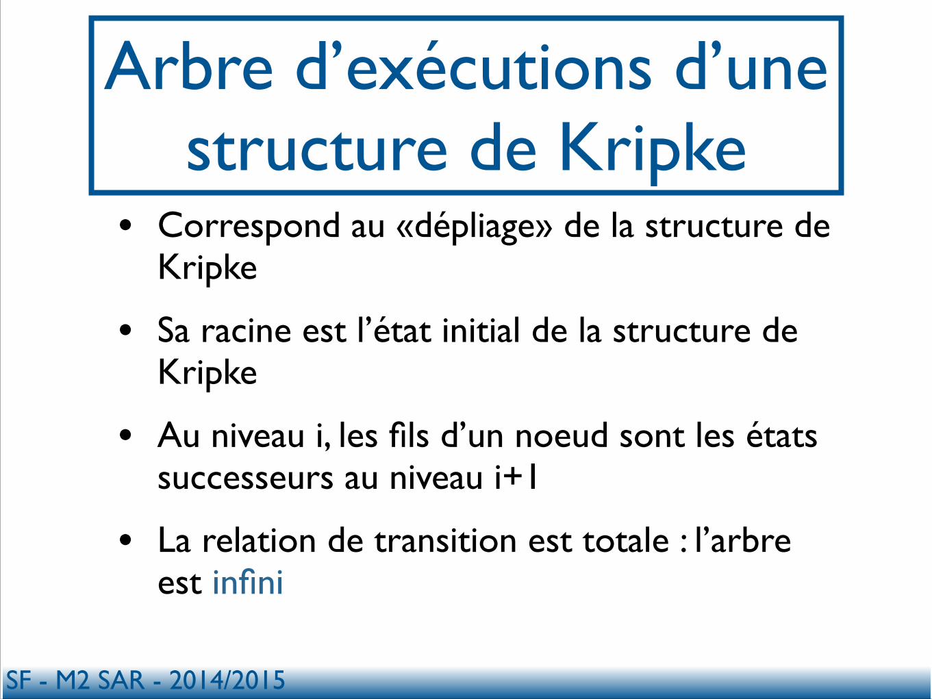
• Correspond au «dépliage» de la structure de Kripke
• Sa racine est l’état initial de la structure de Kripke
• Au niveau i, les fils d’un noeud sont les états successeurs au niveau i+1
• La relation de transition est totale : l’arbre est infini

SF - M2 SAR - 2014/2015
Systèmes concurrents• Compositionnalité des modèles, description modulaire
• Différents modes de synchronisation
• entrelacement
• variables partagées
• communication par rendez-vous (synchrone)
• communication par canaux de communication (asynchrone)
• produit synchrone
• ...
• explosion combinatoire
SF - M2 SAR - 2014/2015
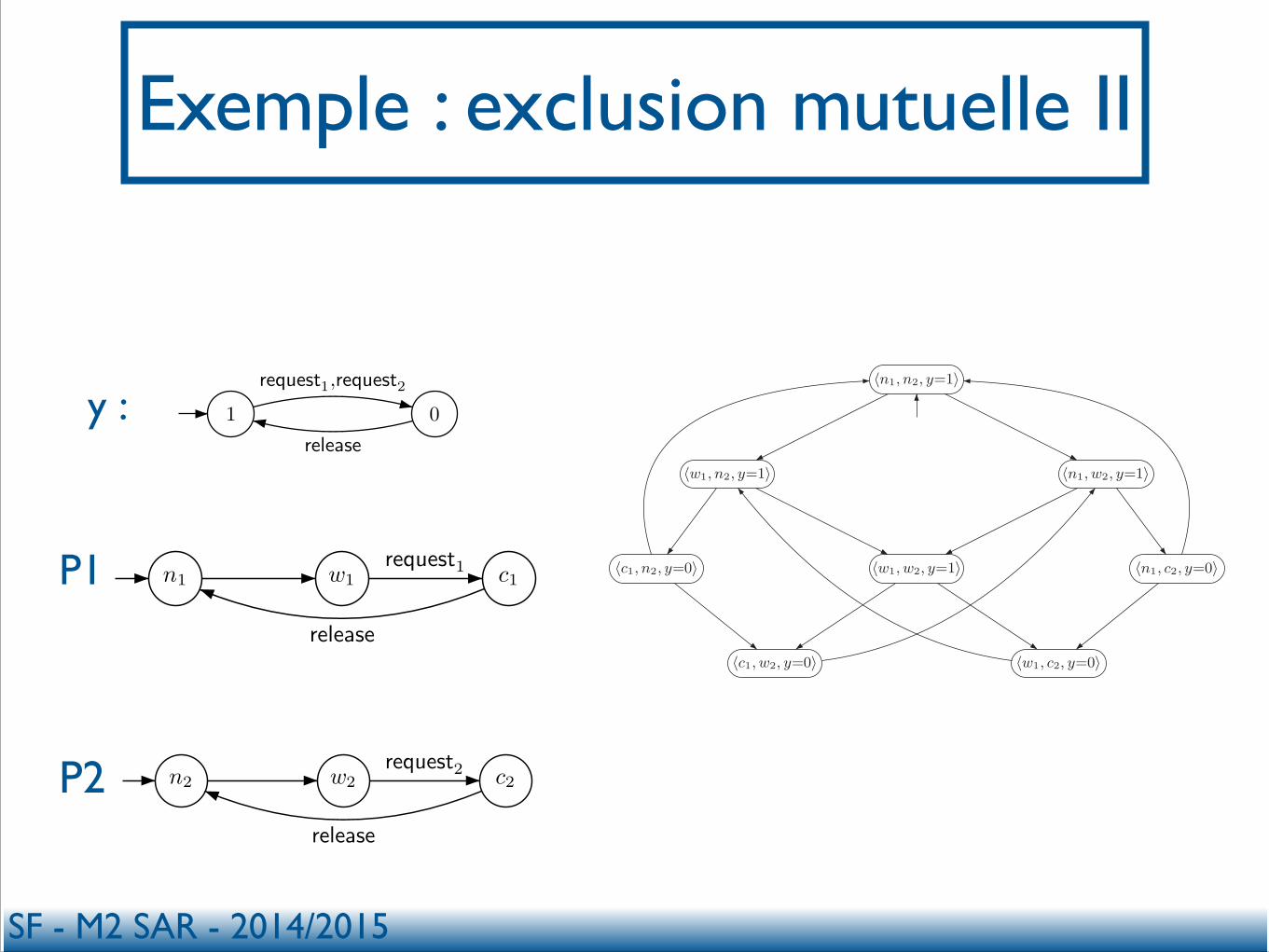
Exemple : exclusion mutuelle II
s0, 0
s1, 1 s2, 1
s3, 2 s3, 2
s1, 3 s3, 3 s1, 3 s3, 3
......
. . .. .. . . .. .
.
01
release
request1,request2
2
n1 w1 c1request1
release
3
n2 w2 c2request2
release
3
y :
P1
P2
Parallelism and Communication 45
⟨n1, n2, y=1⟩
⟨w1, n2, y=1⟩ ⟨n1, w2, y=1⟩
⟨c1, n2, y=0⟩ ⟨w1, w2, y=1⟩ ⟨n1, c2, y=0⟩
⟨c1, w2, y=0⟩ ⟨w1, c2, y=0⟩
Figure 2.8: Mutual exclusion with semaphore (transition system representation).
first-in first-out (FIFO), or some other scheduling discipline can be chosen. Alternatively,another (more concrete) mutual exclusion algorithm could be selected that resolves thisscheduling issue explicitly. A prominent example of such algorithm has been provided in1981 by Peterson [332].
Example 2.25. Peterson’s Mutual Exclusion Algorithm
Consider the processes P1 and P2 with the shared variables b1, b2, and x. b1 and b2 areBoolean variables, while x can take either the value 1 or 2, i.e., dom(x) = { 1, 2 }. Thescheduling strategy is realized using x as follows. If both processes want to enter thecritical section (i.e., they are in location waiti), the value of variable x decides which ofthe two processes may enter its critical section: if x = i, then Pi may enter its criticalsection (for i = 1, 2). On entering location wait1, process P1 performs x := 2, thus givingprivilege to process P2 to enter the critical section. The value of x thus indicates whichprocess has its turn to enter the critical section. Symmetrically, P2 sets x to 1 whenstarting to wait. The variables bi provide information about the current location of Pi.More precisely,
bi = waiti ∨ criti .
bi is set when Pi starts to wait. In pseudocode, P1 performs as follows (the code for processP2 is similar):

SF - M2 SAR - 2014/2015
Descriptifs de haut niveau
• Programmes séquentiels
• Programmes concurrents
• Réseaux de Petri
• ...
SF - M2 SAR - 2014/2015
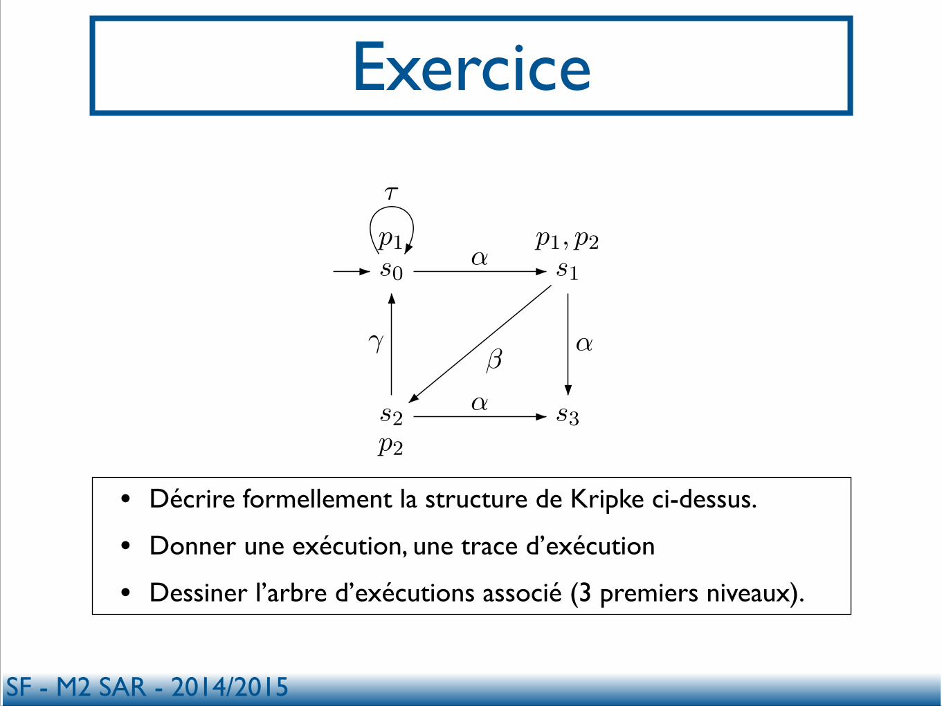
Exercice
• Décrire formellement la structure de Kripke ci-dessus.
• Donner une exécution, une trace d’exécution
• Dessiner l’arbre d’exécutions associé (3 premiers niveaux).
RHEINISCH-WESTFALISCHETECHNISCHEHOCHSCHULEAACHEN
LEHRSTUHL FUR INFORMATIK II
RWTH Aachen · D-52056 Aachen · GERMANY
http://www-i2.informatik.rwth-aachen.de
Prof. Dr. Ir. J.-P. KatoenM. Neuhaußer
Exercises to the lecture “Model Checking”, winter term 2005
– Assignment 1 –
The solutions are collected on Oct. 28th at the beginning of the exercise class.
Exercise 1 (0.5 + 0.5 points)
Consider the following transition system:
s0
p1
s1
p1, p2
s2
p2
s3
α
βγ α
α
τ
(a) Give a formal definition of the transition system outlined above.
(b) Specify a finite and an infinite execution. Is the transition system deterministic?
Exercise 2 (1 + 1 + 2 points)
Consider the following street junction with the specification of a traffic light as outlined on the right.
A1
A3
A1
A2
A2
Ai : red
green
yellow red/yellow
a) Choose appropriate actions and label the transitions of the traffic light transition system accordingly.
b) Give the transition system representation of a (reasonable) controller C that switches the greensignal lamps in the following order: A1, A2, A3, A1, A2, A3, . . . .(Hint: Choose an appropriate communication mechanism)
c) Outline the transition system A1∥A2∥A3∥C.

VFSR - M2 SAR - 2013/2014
2. Spécifications

SF - M2 SAR - 2014/2015
Propriétés sur les systèmes de transition (I)
• Invariance : tous les états du système vérifient une certaine propriété
• Sûreté : quelque chose de mauvais n’arrive jamais
• Accessibilité : un état donné est accessible depuis l’état initial

SF - M2 SAR - 2014/2015
Propriétés sur les systèmes de transition (II)
• Vivacité : Quelque chose de «bon» finira par arriver
• Equité : Quelque chose se produira infiniment souvent

SF - M2 SAR - 2014/2015
Logiques temporelles
• Permettent d’exprimer propriétés sur séquences d’observations
• Utilisation de connecteurs temporels et de quantificateurs sur les chemins

SF - M2 SAR - 2014/2015
Logiques temporelles : pourquoi?
• On pourrait utiliser logique du premier ordre.
• Exemple : «toute requête sera un jour satisfaite»
Figure 1: essai
blablabla'
8t ·�requete ! 9t0 � t · (reponse)
�
1

SF - M2 SAR - 2014/2015
Logiques temporelles : pourquoi?
• On pourrait utiliser logique du premier ordre.
• Exemple : «toute requête sera un jour satisfaite»Difficile à écrire
/comprendre
Vérification peu efficace
Figure 1: essai
blablabla'
8t ·�requete ! 9t0 � t · (reponse)
�
1

SF - M2 SAR - 2014/2015
Logiques temporelles
• Pas de variable (instants implicites), mais modalités.
• Temporel ≠ temporisé : logiques temporelles ne quantifient pas écoulement du temps.

SF - M2 SAR - 2014/2015
Logiques temporelles linéaires ou arborescentes
• 2 approches :
• temps linéaire : propriétés des séquences d’exécutions (futur déterminé)
• temps arborescent : propriétés de l’ arbre d’exécutions (tous les futurs possibles)

VFSR - M2 SAR - 2013/2014
2.2 La logique LTL

SF - M2 SAR - 2014/2015
Logique temporelle linéaire : LTL
• Modèle des formules : une trace d’exécution infinie.
• t, i ⊧ φ ssi la formule φ est vérifiée à la position i de la trace.
• Défini inductivement sur la formule
[Pnueli 77]

SF - M2 SAR - 2014/2015
• Rappel : une trace d’exécution ≣ exécution dans laquelle seul l’étiquetage des états est visible
• → c’est un mot (infini) sur l’alphabet 2AP.
• Soit t une trace, on note t(i) la «lettre» à la position i≥0, i.e. l’ensemble des propositions atomiques vraies.
Logique temporelle linéaire : LTL

SF - M2 SAR - 2014/2015
Logique temporelle linéaire : LTL
p p,q q,rq p,rp :
p pp
...
t,i ⊧ p ssi p∈t(i)

SF - M2 SAR - 2014/2015
Logique temporelle linéaire : LTL
Xφ : ...
Xφ
q,r p,q q,rp p,r ...Exemples : Xp
Xp p
q p q,rq,r p,r ...X(Xp)
φ

SF - M2 SAR - 2014/2015
Logique temporelle linéaire : LTL
Xφ : ...
Xφ
q,r p,q q,rp p,r ...Exemples : Xp
Xp p
q p q,rq,r p,r ...
p
X(Xp) p
φ

SF - M2 SAR - 2014/2015
Logique temporelle linéaire : LTL
Xφ : ...
Xφ
q,r p,q q,rp p,r ...Exemples : Xp
Xp p
q p q,rq,r p,r ...
Xp p
X(Xp) q,r p
φ

SF - M2 SAR - 2014/2015
Logique temporelle linéaire : LTL
Xφ : ...
Xφ
q,r p,q q,rp p,r ...Exemples : Xp
Xp p
q p q,rq,r p,r ...
X(Xp) Xp p
X(Xp) q,rq p
φ

SF - M2 SAR - 2014/2015
Logique temporelle linéaire : LTL
Xφ : ...
Xφ
t,i ⊧ Xφ ssi t,i+1⊧φ
φ

SF - M2 SAR - 2014/2015
Logique temporelle linéaire : LTL
Fφ : ...
φ

SF - M2 SAR - 2014/2015
Logique temporelle linéaire : LTL
Fφ : ...
Fφ
Fφ
φ

SF - M2 SAR - 2014/2015
Logique temporelle linéaire : LTL
Fφ : ...
Fφ Fφ
Fφ
φ

SF - M2 SAR - 2014/2015
Logique temporelle linéaire : LTL
Fφ : ...
Fφ Fφ Fφ
Fφ
φ

SF - M2 SAR - 2014/2015
Logique temporelle linéaire : LTL
Fφ : ...
Fφ Fφ Fφ
Fφ
t,i ⊧ Fφ ssi il existe j≥i tel que t,j⊧φ
φ

SF - M2 SAR - 2014/2015
Logique temporelle linéaire : LTL
Gφ : ...
φ φ φ
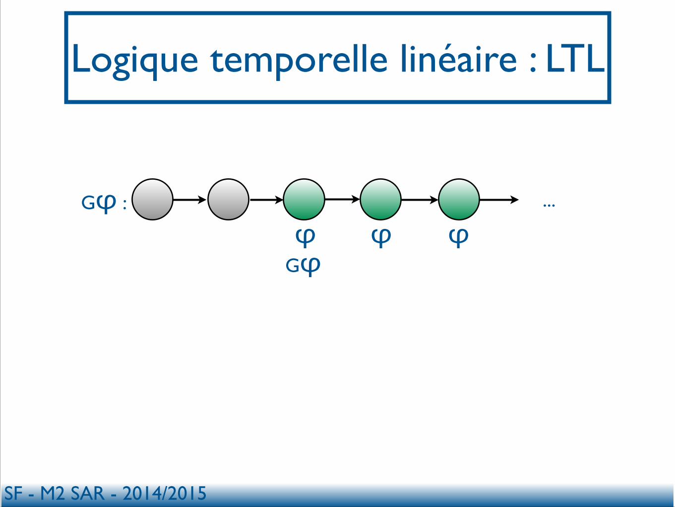
SF - M2 SAR - 2014/2015
Logique temporelle linéaire : LTL
Gφ : ...
Gφ
φ φ φ

SF - M2 SAR - 2014/2015
Logique temporelle linéaire : LTL
Gφ : ...
Gφ
t,i ⊧ Gφ ssi pour tout j≥i, t,j⊧φ
φ φ φ

SF - M2 SAR - 2014/2015
Logique temporelle linéaire : LTL
Gφ : ...
Gφ
t,i ⊧ Gφ ssi pour tout j≥i, t,j⊧φ
φ φ φGφ

SF - M2 SAR - 2014/2015
Logique temporelle linéaire : LTL
Gφ : ...
Gφ
t,i ⊧ Gφ ssi pour tout j≥i, t,j⊧φ
φ φ φGφ Gφ

SF - M2 SAR - 2014/2015
Logique temporelle linéaire : LTL
φ1Uφ2: ...
φ1 φ1 φ2φ1φ1

SF - M2 SAR - 2014/2015
Logique temporelle linéaire : LTL
φ1Uφ2: ...
φ1 φ1 φ2
φ1Uφ2
φ1φ1

SF - M2 SAR - 2014/2015
Logique temporelle linéaire : LTL
φ1Uφ2: ...
t,i ⊧ φ1Uφ2 ssi il existe j≥i, t,j ⊧φ2 et, pour tout i≤k<j, t,k ⊧ φ1
φ1 φ1 φ2
φ1Uφ2
φ1φ1

SF - M2 SAR - 2014/2015
Logique temporelle linéaire : LTL
φ::= p∈AP | ¬φ | φ∨φ |Xφ| Fφ| Gφ| φUφ
t,i ⊧ p ssi p∈t(i) t,i ⊧ ¬φ ssi t,i ⊭ φ t,i ⊧ φ1∨φ2 ssi t,i ⊧ φ1 ou t,i ⊧ φ2
t,i ⊧ Xφ ssi t,i+1⊧φ t,i ⊧ Fφ ssi il existe j≥i tel que t,j⊧φ t,i ⊧ Gφ ssi pour tout j≥i, t,j⊧φ t,i ⊧ φ1Uφ2 ssi il existe j≥i, t,j ⊧φ2 et, pour tout i≤k<j, t,k ⊧ φ1
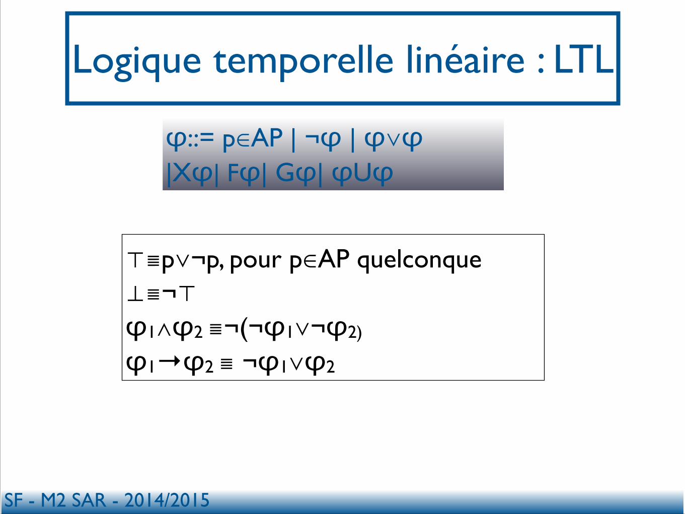
SF - M2 SAR - 2014/2015
Logique temporelle linéaire : LTL
φ::= p∈AP | ¬φ | φ∨φ |Xφ| Fφ| Gφ| φUφ
⊤≣p∨¬p, pour p∈AP quelconque ⊥≣¬⊤ φ1∧φ2 ≣¬(¬φ1∨¬φ2)
φ1→φ2 ≣ ¬φ1∨φ2

SF - M2 SAR - 2014/2015
Logique temporelle linéaire : LTL
En fait, Fφ et Gφ macros aussi : • Fφ≣⊤Uφ • Gφ≣ ¬F(¬φ)
Exercice : vérifier.

SF - M2 SAR - 2014/2015
• Autres macros utiles :
• (Weak until) φ1Wφ2 ≣ Gφ1 ∨ φ1Uφ2
• (Release) φ1Rφ2 ≣ φ2 W (φ1∧φ2) ≣ Gφ2
∨ φ2U (φ1∧φ2)
Logique temporelle linéaire : LTL
φ::= p∈AP | ¬φ | φ∨φ |Xφ| φUφ

SF - M2 SAR - 2014/2015
• Accessibilité : F (x=0)
• Invariance : G ¬(x=0)
• Vivacité : G(request → F response)
• Equité forte : GF enabled → GF scheduled
• Equité faible : FG enabled → GF scheduled
• Relâchement de contrainte : reset R alarm
LTL : Exemples

SF - M2 SAR - 2014/2015
• Toute requête sera un jour satisfaite (AP = {requete, reponse})
• A chaque fois que de l’argent a été retiré, le code pin a été fourni (AP={cash-withdraw, pin-ok})
• Deux processus ne sont jamais en section critique en même temps (AP= {critique1, critique2})
• Si un processus demande l’accès en section critique, il l’obtiendra un jour (AP = {demande_crit, acc_crit})
• Une fois que le feu est vert, il ne peut pas devenir rouge immédiatement (AP= {vert, rouge})
• Lorsque le feu est rouge, il deviendra vert un jour
• Lorsque le feu est vert, il deviendra rouge un jour, après avoir été orange (AP= {vert, rouge, orange})
LTL : Exercice I

SF - M2 SAR - 2014/2015
• Vérifier que ¬Xφ≣X¬φ, ¬(φ1Uφ2)≣ ¬φ1R¬φ2
• Dites si, à chaque position de la trace ci-dessous, les propositions suivantes sont vérifiées : p∧q, F(p∧q), pUq.
LTL : Exercice II
∅ {p} ∅{p}{q} {p,q{p,q}

SF - M2 SAR - 2014/2015
• Les équivalences suivantes sont-elles vraies?
• G(Fp∧Fq) ↔ GFp∧GFq
• F(Gp∧Gq) ↔FGp∧FGq
• G(Fp∨Fq)↔GFp∨GFq
• F(Gp∨Gq)↔FGp∨FGq
• GF(p∧q)↔GFp∧GFq
• GF(p∨q)↔GFp∨GFq
• FG(p∧q)↔FGp∧FGq
• FG(p∨q)↔FGp∨FGq
LTL : Exercice III

VFSR - M2 SAR - 2013/2014
2.3 CTL

SF - M2 SAR - 2014/2015
Exprimer la possibilité• La propriété «à chaque fois que paid est
vérifié, il est possible d’obtenir une bière» n’est pas exprimable en LTL!
Transition Systems 21
the likelihood with which a certain transition is selected. Similarly, when the set of initialstates consists of more than one state, the start state is selected nondeterministically.
The labeling function L relates a set L(s) ∈ 2AP of atomic propositions to any state s.1
L(s) intuitively stands for exactly those atomic propositions a ∈ AP which are satisfiedby state s. Given that Φ is a propositional logic formula, then s satisfies the formula Φ ifthe evaluation induced by L(s) makes the formula Φ true; that is:
s |= Φ iff L(s) |= Φ.
(Basic principles of propositional logic are explained in Appendix A.3, see page 915 ff.)
Example 2.2. Beverage Vending Machine
We consider an (somewhat foolish) example, which has been established as standard in thefield of process calculi. The transition system in Figure 2.1 models a preliminary designof a beverage vending machine. The machine can either deliver beer or soda. States arerepresented by ovals and transitions by labeled edges. State names are depicted inside theovals. Initial states are indicated by having an incoming arrow without source.
pay
selectsoda beer
insert coin
ττ
get soda get beer
Figure 2.1: A transition system of a simple beverage vending machine.
The state space is S = { pay , select , soda , beer }. The set of initial states consists ofonly one state, i.e., I = { pay }. The (user) action insert coin denotes the insertion of acoin, while the (machine) actions get soda and get beer denote the delivery of soda andbeer, respectively. Transitions of which the action label is not of further interest here,e.g., as it denotes some internal activity of the beverage machine, are all denoted by thedistinguished action symbol τ . We have:
Act = { insert coin , get soda , get beer , τ }.
Some example transitions are:
pay insert coin−−−−−−−−→ select and beer get beer−−−−−−→ pay .
1Recall that 2AP denotes the power set of AP.
{paid, soda}
{paid, beer}
{paid}
n2 w2 c2request2
release
pay
select select’
soda beer
insert coin
insert coin
τ τ
get soda get beer
3
{paid, beer}
{paid} {paid}
{paid, soda}
Les deux systèmes vérifient les mêmes propriétés LTL!!

SF - M2 SAR - 2014/2015
Computational Tree Logic : CTL
• Modèle des formules : état de l’arbre d’exécutions infini.
• M,s ⊧ φ ssi la formule φ est vérifiée à l’état s de la structure de Kripke M.
• On note S(φ) l’ensemble des états s t.q. M,s ⊧ φ
• Ajout de quantificateurs sur les chemins dans l’arbre : E et A.
• Défini inductivement sur la formule.
[Clarke, Emerson 81]

SF - M2 SAR - 2014/2015
CTL: syntaxe et sémantique
p
q,r p
r,s p,q q s
s ⊧ p ssi p∈l(s)

SF - M2 SAR - 2014/2015
CTL: syntaxe et sémantique
s ⊧ EXφ ssi il existe s’, successeur de s t.q. s’ ⊧φ
EXφ
φ

SF - M2 SAR - 2014/2015
CTL: syntaxe et sémantique
s ⊧ AXφ ssi pour tout s’, successeur de s, s’ ⊧φ
AXφ
φφ

SF - M2 SAR - 2014/2015
CTL: syntaxe et sémantique
s ⊧ EφUφ’ ssi il existe une exécution s0s1...sk telle que s0=s, sk ⊧φ’ et pour tout 0≤i<k, si ⊧φ.
EφUφ’
φ
φ
φ’

SF - M2 SAR - 2014/2015
CTL: syntaxe et sémantique
s ⊧ AφUφ’ ssi pour toute exécution s0s1... telle que s0=s, ∃ k t.q. sk
⊧φ’ et pour tout 0≤i<k, si ⊧φ.
AφUφ’
φ
φ
φ’
φ’
φ’
φ’
φ

SF - M2 SAR - 2014/2015
CTL: syntaxe et sémantique
φ::= p∈AP | ¬φ | φ∨φ |EXφ| AXφ| EφUφ | AφUφ
s ⊧ p ssi p∈l(s) s ⊧ ¬φ ssi s ⊭ φ s ⊧ φ1∨φ2 ssi s ⊧ φ1 ou s ⊧ φ2
s ⊧ EXφ ssi il existe s’, successeur de s, t.q. s’⊧φ s ⊧ AXφ ssi s’, pour tout s’, successeur de s, s’⊧φ s ⊧ Eφ1Uφ2 ssi il existe une exécution s0s1...sk tel que s0=s, sk ⊧φ2 et pour tout 0≤i≤k, si ⊧φ1. s ⊧ Aφ1Uφ2 ssi pour toute exécution s0s1... telle que s0=s, il existe k t.q. sk ⊧φ2 et pour tout 0≤i≤k, si ⊧φ1.

SF - M2 SAR - 2014/2015
CTL : macros
• EFφ ≣ E⊤Uφ
• AFφ≣A⊤Uφ
• EGφ≣¬AF¬φ
• AGφ≣¬EF¬φ

SF - M2 SAR - 2014/2015
CTL : Equivalences de formules
• AXφ=¬EX¬φ
• AφUφ’=¬E¬(φUφ’)=¬E(G¬φ’∨¬φ’U(¬φ∧¬φ’))=¬EG¬φ’∧¬E(¬φ’U(¬φ∧¬φ’))

SF - M2 SAR - 2014/2015
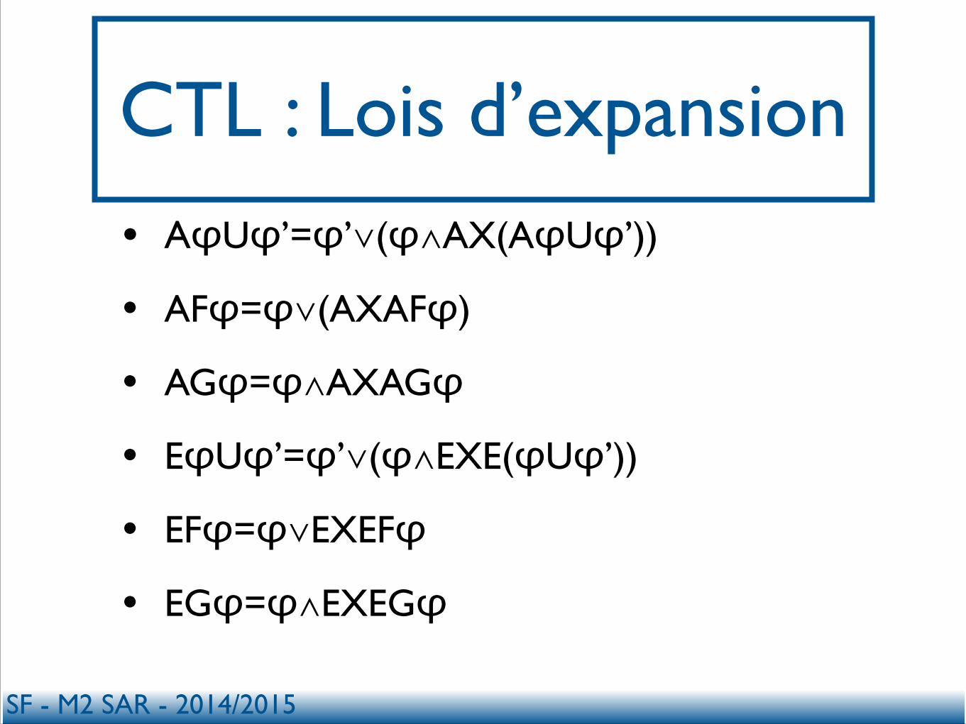
CTL : Lois d’expansion• AφUφ’=φ’∨(φ∧AX(AφUφ’))
• AFφ=φ∨(AXAFφ)
• AGφ=φ∧AXAGφ
• EφUφ’=φ’∨(φ∧EXE(φUφ’))
• EFφ=φ∨EXEFφ
• EGφ=φ∧EXEGφ

SF - M2 SAR - 2014/2015
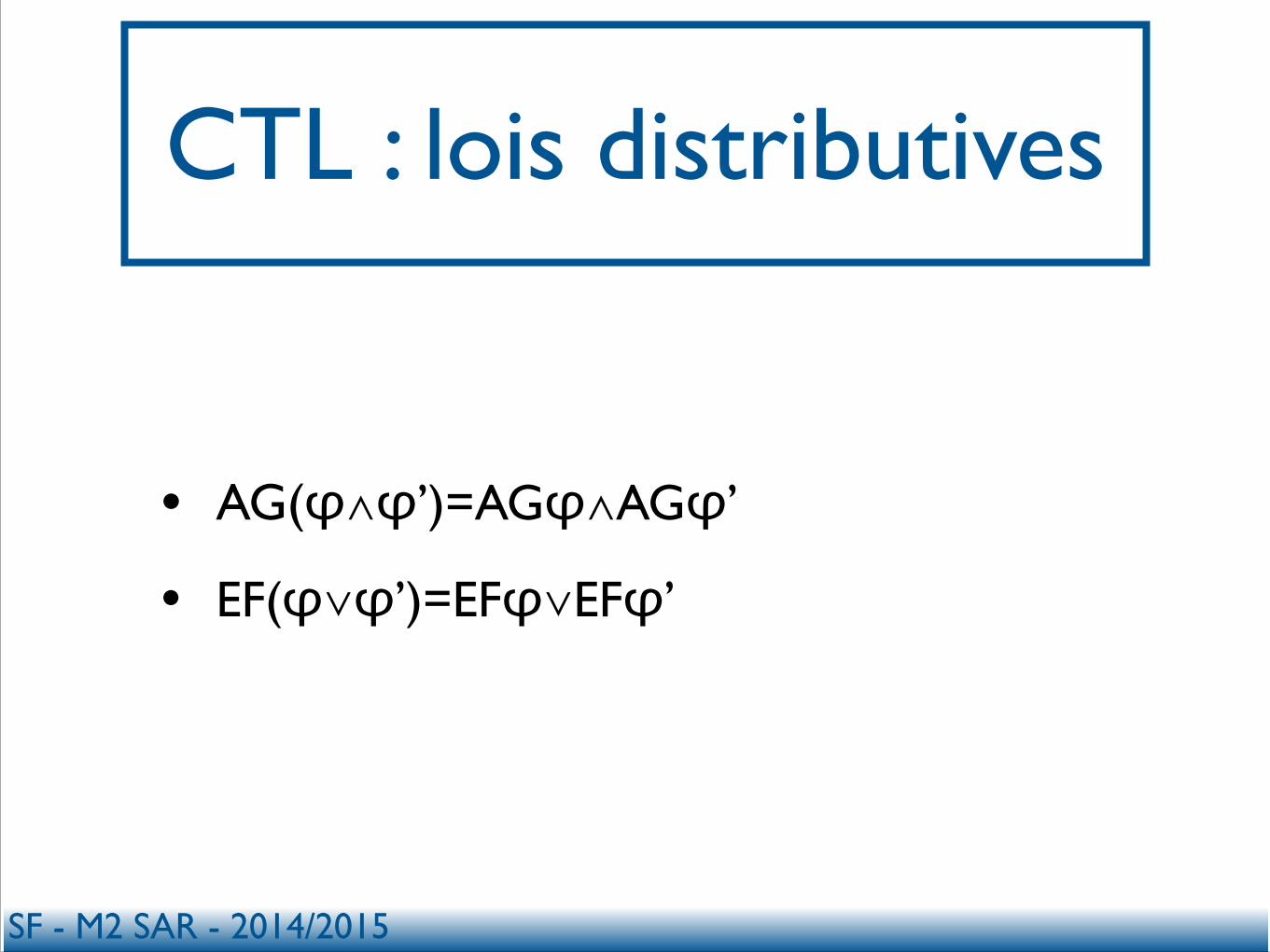
CTL : lois distributives
• AG(φ∧φ’)=AGφ∧AGφ’
• EF(φ∨φ’)=EFφ∨EFφ’

SF - M2 SAR - 2014/2015
Exemples
• Accessibilité : EF(x=0)
• Invariance : AG¬(x=0)
• Vivacité : AGAF(active)

SF - M2 SAR - 2014/2015
Exercice
61/71
CTL (Clarke & Emerson 81)
Example
1 2 3 4
5 6 7 8
q p, q q r
p, r p, r p, q
Compute
S(EX p) = {1, 2, 3, 5, 6}
S(AX p) = {3, 6}
S(EF p) = {1, 2, 3, 4, 5, 6, 7, 8}
S(AF p) = {2, 3, 5, 6, 7}
S(E q U r) =
S(A q U r) =
S(EXp)? S(AXp)? S(EFp)? S(AFp)? S(EqUr)?S(AqUr)?

SF - M2 SAR - 2014/2015
Exercice• Toute fraude est susceptible d’être détectée un jour(AP={fraude,
detect})
• Deux processus ne sont jamais en section critique en même temps (AP={crit1,crit2})
• Toute requête sera un jour satisfaite (AP = {requete, reponse})
• Le processus est activé infiniment souvent (AP= {active})
• Il est possible qu’à partir d’un moment, l’alarme sonne continuellement (AP= {alarm})
• La lumière finit toujours par s’éteindre (AP= {off})
• La lumière finit toujours par s’éteindre et la ventilation tourne tant que la lumière est allumée (AP= {ventilation,off})

SF - M2 SAR - 2014/2015
Comparaison LTL/CTL
• La formule CTL AF(a∧EXa) n’est pas exprimable en LTL
• La formule LTL FG request →GF response n’est pas exprimable en CTL
• LTL et CTL incomparables!
• LTL et CTL inclus dans CTL*

VFSR - M2 SAR - 2013/2014
3.Algorithmes de Model-Checking

SF - M2 SAR - 2014/2015
Model-Checking de LTL
• Données : Une structure de Kripke M=(Q,T, A, q0, AP, l) et une formule LTL φ.
• Question : Est-ce que M ⊧ φ?
• M ⊧ φ ssi t,0 ⊧ φ pour toute trace initiale t de M.

SF - M2 SAR - 2014/2015
ExerciceExercise 3 (3 points)
Consider the transition system TS over the set of atomic propositions AP = {a, b, c}:
s1
{a}
s3
{b, c}
s2
{c}
s5
{a, b, c}
s4
{b}
Decide for each of the LTL formulas ϕi below, whether TS |= ϕi holds. Justify your answers! If TS |= ϕi,provide a path π ∈ Paths(TS) such that π |= ϕi.
ϕ1 = ✸✷c
ϕ2 = ✷✸c
ϕ3 =⃝¬c →⃝⃝c
ϕ4 = ✷a
ϕ5 = aU✷(b ∨ c)
ϕ6 = (⃝⃝b)U(b ∨ c)
M⊧φ?
• φ=FGc
• φ=GFc
• φ=Ga
• φ=aU(G(b∨c))
• X¬c→XXc

SF - M2 SAR - 2014/2015
Model-Checking de LTL: principe
• Soit Σ un alphabet. On note Σ* l’ensemble des mots finis et Σ les mots infinis.
• Modèles de φ = mots infinis. Soit ⟦φ⟧ le langage
des modèles de la formule : ⟦φ⟧={t∈(2AP) | t, 0⊧ φ}
• Soit ⟦M⟧ le langage des traces initiales de M :⟦M⟧= {t∈ (2AP) | t est une trace initiale de M}
• Le problème du model-checking revient donc à vérifier si : ⟦M⟧⊆⟦φ⟧
Figure 1: essai
blablabla'
8t ·�requete ! 9t0 � t · (reponse)
�
!
1
Figure 1: essai
blablabla'
8t ·�requete ! 9t0 � t · (reponse)
�
!
1
Figure 1: essai
blablabla'
8t ·�requete ! 9t0 � t · (reponse)
�
!
1

SF - M2 SAR - 2014/2015
Outil : les automates de Büchi
• Définition : Un automate de Büchi est un n-uplet A=(Q, Σ, I, T, F) avec
• Q un ensemble fini d’états
• Σ un alphabet fini
• I⊆Q les états initiaux
• T⊆Q x Σ x Q la relation de transition
• F⊆Q un ensemble d’états acceptants (ou répétés)

SF - M2 SAR - 2014/2015
Outil : les automates de Büchi
• Une exécution de A sur un mot infini w=w0w1w2... de Σ est une séquence r=q0q1q2q3... telle que q0∈I et (qi,wi,qi+1)∈T, pour tout i≥0.
• r est acceptante si qi∈F pour un nombre infini de i.
• w est accepté par A s’il existe une exécution acceptante de A sur w.
• L(A)={w∈ Σ | w accepté par A}.
Figure 1: essai
blablabla'
8t ·�requete ! 9t0 � t · (reponse)
�
!
1
Figure 1: essai
blablabla'
8t ·�requete ! 9t0 � t · (reponse)
�
!
1

SF - M2 SAR - 2014/2015
Automate de Büchi: exemple
38/71
Buchi automata
Definition
A = (Q, Σ, I, T, F ) where
! Q: finite set of states
! Σ: finite set of labels
! I ⊆ Q: set of initial states
! T ⊆ Q× Σ×Q: transitions
! F ⊆ Q: set of accepting states (repeated, final)
Example
A = 1 2
a b
b
a
L(A) = {w ∈ {a, b}ω | |w|a = ω}

SF - M2 SAR - 2014/2015
Automate de Büchi: exemple
Introduction
A= 1 2
a, b
b
b
L(A)?
Master SAR - VFSR - 2011-2012 , p.4

SF - M2 SAR - 2014/2015
Automates de Büchi non-déterministes
• Les automates de Büchi non déterministes sont plus expressifs que les automates de Büchi déterministes
• Les langages reconnus par un NBA forment les -réguliers
• Toute formule de LTL peut être reconnue par un NBA
s0
s1 s2
s3
Figure 1: essai
blablablaϕ
∀t ·!
requete → ∃t′ ≥ t · (reponse)"
ω
1

SF - M2 SAR - 2014/2015
Les automates de Büchi pour LTL
• Définition : Un automate de Büchi est un n-uplet A=(Q, Σ, I, T, F) avec
• Q un ensemble fini d’états
• Σ un alphabet fini
• I⊆Q les états initiaux
• T⊆Q x Σ x Q la relation de transition
• F⊆Q un ensemble d’états acceptants (ou répétés)

SF - M2 SAR - 2014/2015
Les automates de Büchi pour LTL
• Définition : Un automate de Büchi est un n-uplet A=(Q, Σ, I, T, F) avec
• Q un ensemble fini d’états
• Σ un alphabet fini
• I⊆Q les états initiaux
• T⊆Q x Σ x Q la relation de transition
• F⊆Q un ensemble d’états acceptants (ou répétés)
Σ = 2AP

SF - M2 SAR - 2014/2015
Exercice
• Exemple : automate de Büchi reconnaissant p, Xp.
• Construire des automates de Büchi reconnaissant Fp, XXp, Gp, FGp, GFp, pUq, pRq.

SF - M2 SAR - 2014/2015
Automates de Büchi et LTL
• Les formules de LTL sont moins expressives que les automates de Büchi
• Exemple : «Un instant sur deux, l’événement a arrive.» est une propriété régulière non exprimable en LTL
s0
s1 s2
s3
Figure 1: essai
blablablaϕ
∀t ·!
requete → ∃t′ ≥ t · (reponse)"
ω
1

SF - M2 SAR - 2014/2015
Automates de Büchi
Théorème : Les automates de Büchi sont clos par union, intersection, et complément.
Théorème : on peut tester le vide d’un automate de Büchi.

SF - M2 SAR - 2014/2015
• Chercher si un état acceptant est accessible depuis l’état initial
• Chercher si cet état appartient à un cycle
Automates de Büchi - Test du vide

SF - M2 SAR - 2014/2015
Model-Checking LTL : approche par automates• Donnée: Structure de Kripke M, formule LTL φ.
• Etapes de l’algorithme :
• Transformer M en un automate AM tel que L(AM)=⟦M⟧ (assez facile)
• Transformer φ en un automate Aφ tel que L(Aφ)=⟦φ⟧ (plus difficile)
• Tester si L(AM)⊆ L(Aφ), i.e., si L(AM)∩L(Aφ)c=∅.
Difficile de co
mplémenter un automate
de Büchi!!
SF - M2 SAR - 2014/2015
Model-Checking LTL : approche par automates• Donnée: Structure de Kripke M, formule LTL φ.
• Etapes de l’algorithme :
• Transformer M en un automate AM tel que L(AM)=⟦M⟧
• Transformer φ en un automate A¬φ tel que L(A¬φ)=⟦¬φ⟧
• Tester si L(AM)∩L(A¬φ)=∅.

SF - M2 SAR - 2014/2015
Transformer φ en un automate de Büchi
1. Automates de Büchi généralisés
2. Réduire la formule
1. Forme normale négative
2. Réduire les connecteurs temporels
3. Transformation en automate de Büchi généralisé

SF - M2 SAR - 2014/2015
Transformer φ en un automate de Büchi
1. Automates de Büchi généralisés
2. Réduire la formule
1. Forme normale négative
2. Réduire les connecteurs temporels
3. Transformation en automate de Büchi généralisé

SF - M2 SAR - 2014/2015
Automates de Büchi généralisés
• Définition : Un automate de Büchi généralisé est un n-uplet A=(Q, Σ, I, T, F) avec
• Q un ensemble fini d’états
• Σ un alphabet fini
• I⊆Q les états initiaux
• T⊆Q x Σ x Q la relation de transition
• F={F1,F2,...,Fk}⊆2Q un ensemble d’ensemble d’états acceptants (ou répétés)

SF - M2 SAR - 2014/2015
• Une exécution de A sur un mot infini w=w0w1w2... de Σ est une séquence r=q0q1q2q3... telle que q0∈I et (qi,wi,qi+1)∈T, pour tout i≥0.
• r est acceptante si pour tout F∈F, qi∈F pour un nombre infini de i.
• w est accepté par A s’il existe une exécution acceptante de A sur w.
• L(A)={w∈ Σ | w accepté par A}.
Automates de Büchi généralisésFigure 1: essai
blablabla'
8t ·�requete ! 9t0 � t · (reponse)
�
!
1
Figure 1: essai
blablabla'
8t ·�requete ! 9t0 � t · (reponse)
�
!
1

SF - M2 SAR - 2014/2015
Automates de Büchi généralisés : exemple
44/71
Generalized Buchi automataDefinition: acceptance on states
A = (Q, Σ, I, T, F1, . . . , Fn) with Fi ⊆ Q.
An infinite run σ is successful if it visits infinitely often each Fi.
G F p ∧ GF q: 0
ΣΣp
ΣΣq
Σ
Definition: acceptance on transitions
A = (Q, Σ, I, T, T1, . . . , Tn) with Ti ⊆ T .
An infinite run σ is successful if it uses infinitely many transitions from each Ti.
G F p ∧ GF q:
GFp∧GFq:

SF - M2 SAR - 2014/2015
Des ABG aux AB
Théorème : Tout automate de Büchi généralisé A peut être transformé en un automate de Büchi A’
tel que L(A)=L(A’)

SF - M2 SAR - 2014/2015
Transformer φ en un automate de Büchi
1. Automates de Büchi généralisés
2. Réduire la formule
1. Forme normale négative
2. Réduire les connecteurs temporels
3. Transformation en automate de Büchi généralisé

SF - M2 SAR - 2014/2015
Forme normale négativeφ ::= ⊥ | ⊤ | p | ¬p | φ∨φ | φ∧φ |
Xφ | φUφ | φRφ
•¬¬p=p •¬(φ1∨φ2)=¬φ1∧¬φ2
• ¬(φ1∧φ2)=¬φ1∨¬φ2 •¬(Xφ)=X(¬φ) •¬(φ1Uφ2)=¬φ1R¬φ2 •¬(φ1Rφ2)=¬φ1U¬φ2

SF - M2 SAR - 2014/2015
Exercice
• Transformer G(p→Fq) en forme normale négative

SF - M2 SAR - 2014/2015
Réduire les connecteurs temporels
• Idée : Un état de notre graphe va représenter l’ensemble des propositions atomiques vérifiées au prochain instant de la séquence, et l’ensemble des sous-formules qu’il «promet» de vérifier à l’état suivant.
• Pour cela, on ne veut que des propositions atomiques (ou négations), et des sous-formules commençant par X (next).

SF - M2 SAR - 2014/2015
Réduire les connecteurs temporels
• Un ensemble Z de formules en forme normale négative est réduit si
(1) pour tout z∈Z, z est de la forme p, ¬p ou X(z’)
(2) il est cohérent : ⊥∉Z, {p,¬p}⊈Z, pour tout p∈AP.

SF - M2 SAR - 2014/2015
Réduire les connecteurs temporels
• On utilise les équivalences suivantes :
• φUφ’ ≣ φ’∨(φ∧X(φUφ’))
• φRφ’ ≣ (φ∧φ’)∨(φ’∧X(φRφ’))

SF - M2 SAR - 2014/2015
Construction du graphe de réduction

SF - M2 SAR - 2014/2015
Construction du graphe de réduction
Z U {φ∨φ’}
Z U {φ} Z U {φ’}

SF - M2 SAR - 2014/2015
Construction du graphe de réduction
Z U {φ∨φ’}
Z U {φ} Z U {φ’}
Z U {φ∧φ’}
Z U {φ,φ’}

SF - M2 SAR - 2014/2015
Construction du graphe de réduction
Z U {φ∨φ’}
Z U {φ} Z U {φ’}
Z U {φ∧φ’}
Z U {φ,φ’}
Z U {φUφ’}
Z U {φ’} Z U {φ,X(φUφ’)}

SF - M2 SAR - 2014/2015
Construction du graphe de réduction
Z U {φ∨φ’}
Z U {φ} Z U {φ’}
Z U {φ∧φ’}
Z U {φ,φ’}
Z U {φUφ’}
Z U {φ’} Z U {φ,X(φUφ’)}
Z U {φRφ’}
Z U {φ,φ’} Z U {φ’,X(φRφ’)}

SF - M2 SAR - 2014/2015
Exemple de réduction d’une formule
(pUq)∧(¬rUs)(pUq)∧(¬rUs)

SF - M2 SAR - 2014/2015
Exemple de réduction d’une formule
(pUq)∧(¬rUs)(pUq)∧(¬rUs)
pUq, ¬rUs

SF - M2 SAR - 2014/2015
Exemple de réduction d’une formule
(pUq)∧(¬rUs)(pUq)∧(¬rUs)
pUq, ¬rUs
p,X(pUq), ¬rUs

SF - M2 SAR - 2014/2015
Exemple de réduction d’une formule
(pUq)∧(¬rUs)(pUq)∧(¬rUs)
pUq, ¬rUs
p,X(pUq), ¬rUs q, ¬rUs

SF - M2 SAR - 2014/2015
Exemple de réduction d’une formule
(pUq)∧(¬rUs)(pUq)∧(¬rUs)
pUq, ¬rUs
p,X(pUq), ¬rUs q, ¬rUs
p,X(pUq), s

SF - M2 SAR - 2014/2015
Exemple de réduction d’une formule
(pUq)∧(¬rUs)(pUq)∧(¬rUs)
pUq, ¬rUs
p,X(pUq), ¬rUs q, ¬rUs
p,X(pUq), ¬r, X(¬rUs) p,X(pUq), s

SF - M2 SAR - 2014/2015
Exemple de réduction d’une formule
(pUq)∧(¬rUs)(pUq)∧(¬rUs)
pUq, ¬rUs
p,X(pUq), ¬rUs q, ¬rUs
p,X(pUq), ¬r, X(¬rUs) p,X(pUq), s q, s

SF - M2 SAR - 2014/2015
Exemple de réduction d’une formule
(pUq)∧(¬rUs)(pUq)∧(¬rUs)
pUq, ¬rUs
p,X(pUq), ¬rUs q, ¬rUs
p,X(pUq), ¬r, X(¬rUs) p,X(pUq), s q, ¬r, X(¬r Us) q, s

SF - M2 SAR - 2014/2015
Transformer φ en un automate de Büchi
1. Automates de Büchi généralisés
2. Réduire la formule
1. Forme normale négative
2. Réduire les connecteurs temporels
3. Transformation en automate de Büchi généralisé

SF - M2 SAR - 2014/2015
Exemple (suite)(pUq)∧(¬rUs)
pUq, ¬rUs
p,X(pUq), ¬rUs q, ¬rUs
p,X(pUq), ¬r, X(¬rUs)
p,X(pUq), s q, ¬r, X(¬r Us) q, s

SF - M2 SAR - 2014/2015
Exemple (suite)(pUq)∧(¬rUs)
pUq, ¬rUs
p,X(pUq), ¬rUs q, ¬rUs
p,X(pUq), ¬r, X(¬rUs)
p,X(pUq), s q, ¬r, X(¬r Us) q, s
Σp∧¬r

SF - M2 SAR - 2014/2015
Exemple (suite)(pUq)∧(¬rUs)
pUq, ¬rUs
p,X(pUq), ¬rUs q, ¬rUs
p,X(pUq), ¬r, X(¬rUs)
p,X(pUq), s q, ¬r, X(¬r Us) q, s
Σp∧¬r
Σp∧s
pUq

SF - M2 SAR - 2014/2015
Exemple (suite)(pUq)∧(¬rUs)
pUq, ¬rUs
p,X(pUq), ¬rUs q, ¬rUs
p,X(pUq), ¬r, X(¬rUs)
p,X(pUq), s q, ¬r, X(¬r Us) q, s
Σp∧¬r
Σp∧s
pUqΣq∧¬r
¬rUs

SF - M2 SAR - 2014/2015
Exemple (suite)(pUq)∧(¬rUs)
pUq, ¬rUs
p,X(pUq), ¬rUs q, ¬rUs
p,X(pUq), ¬r, X(¬rUs)
p,X(pUq), s q, ¬r, X(¬r Us) q, s
Σp∧¬r
Σp∧s
pUqΣq∧¬r
¬rUs ∅
Σq∧ s

SF - M2 SAR - 2014/2015
Exemple (suite)(pUq)∧(¬rUs)
pUq, ¬rUs
p,X(pUq), ¬rUs q, ¬rUs
p,X(pUq), ¬r, X(¬rUs)
p,X(pUq), s q, ¬r, X(¬r Us) q, s
Σp∧¬r
Σp∧s
pUqΣq∧¬r
¬rUs ∅
Σq∧ s

SF - M2 SAR - 2014/2015
Exemple (suite)(pUq)∧(¬rUs)
pUq, ¬rUs
p,X(pUq), ¬rUs q, ¬rUs
p,X(pUq), ¬r, X(¬rUs)
p,X(pUq), s q, ¬r, X(¬r Us) q, s
Σp∧¬r
Σp∧s
pUqΣq∧¬r
¬rUs ∅
Σq∧ s
p,X(pUq) q

SF - M2 SAR - 2014/2015
Exemple (suite)(pUq)∧(¬rUs)
pUq, ¬rUs
p,X(pUq), ¬rUs q, ¬rUs
p,X(pUq), ¬r, X(¬rUs)
p,X(pUq), s q, ¬r, X(¬r Us) q, s
Σp∧¬r
Σp∧s
pUqΣq∧¬r
¬rUs ∅
Σq∧ s
p,X(pUq) q ¬r,X(¬rUs) s

SF - M2 SAR - 2014/2015
Exemple (suite)(pUq)∧(¬rUs)
pUq, ¬rUs
p,X(pUq), ¬rUs q, ¬rUs
p,X(pUq), ¬r, X(¬rUs)
p,X(pUq), s q, ¬r, X(¬r Us) q, s
Σp∧¬r
Σp∧s
pUqΣq∧¬r
¬rUs ∅
Σq∧ s
p,X(pUq) q ¬r,X(¬rUs) s
Σp

SF - M2 SAR - 2014/2015
Exemple (suite)(pUq)∧(¬rUs)
pUq, ¬rUs
p,X(pUq), ¬rUs q, ¬rUs
p,X(pUq), ¬r, X(¬rUs)
p,X(pUq), s q, ¬r, X(¬r Us) q, s
Σp∧¬r
Σp∧s
pUqΣq∧¬r
¬rUs ∅
Σq∧ s
p,X(pUq) q ¬r,X(¬rUs) s
Σp
Σq

SF - M2 SAR - 2014/2015
Exemple (suite)(pUq)∧(¬rUs)
pUq, ¬rUs
p,X(pUq), ¬rUs q, ¬rUs
p,X(pUq), ¬r, X(¬rUs)
p,X(pUq), s q, ¬r, X(¬r Us) q, s
Σp∧¬r
Σp∧s
pUqΣq∧¬r
¬rUs ∅
Σq∧ s
p,X(pUq) q ¬r,X(¬rUs) s
Σp
Σq
Σ¬r

SF - M2 SAR - 2014/2015
Exemple (suite)(pUq)∧(¬rUs)
pUq, ¬rUs
p,X(pUq), ¬rUs q, ¬rUs
p,X(pUq), ¬r, X(¬rUs)
p,X(pUq), s q, ¬r, X(¬r Us) q, s
Σp∧¬r
Σp∧s
pUqΣq∧¬r
¬rUs ∅
Σq∧ s
p,X(pUq) q ¬r,X(¬rUs) s
Σp
ΣqΣs
Σ¬r

SF - M2 SAR - 2014/2015
Exemple (suite)(pUq)∧(¬rUs)
pUq, ¬rUs
p,X(pUq), ¬rUs q, ¬rUs
p,X(pUq), ¬r, X(¬rUs)
p,X(pUq), s q, ¬r, X(¬r Us) q, s
Σp∧¬r
Σp∧s
pUqΣq∧¬r
¬rUs ∅
Σq∧ s
p,X(pUq) q ¬r,X(¬rUs) s
Σp
Σ
ΣqΣs
Σ¬r

SF - M2 SAR - 2014/2015
Exemple (suite)(pUq)∧(¬rUs)
pUq, ¬rUs
p,X(pUq), ¬rUs q, ¬rUs
p,X(pUq), ¬r, X(¬rUs)
p,X(pUq), s q, ¬r, X(¬r Us) q, s
Σp∧¬r
Σp∧s
pUqΣq∧¬r
¬rUs ∅
Σq∧ s
p,X(pUq) q ¬r,X(¬rUs) s
Σp
Σ
ΣqΣs
Σ¬r

SF - M2 SAR - 2014/2015
Exemple (fin)
StartError
CloseCloseHeat
StartCloseError
StartClose
StartCloseHeat
start oven
close door
close door
open door
start oven
open door
done
cook
open doorreset
warmup
start cooking
1
2 3 4
(p, s)(q,¬r)
(q, s)
(p,¬r)
p
¬r
Σ
q
s
4
FpUq={3,4} F¬rUs={2,4}

SF - M2 SAR - 2014/2015
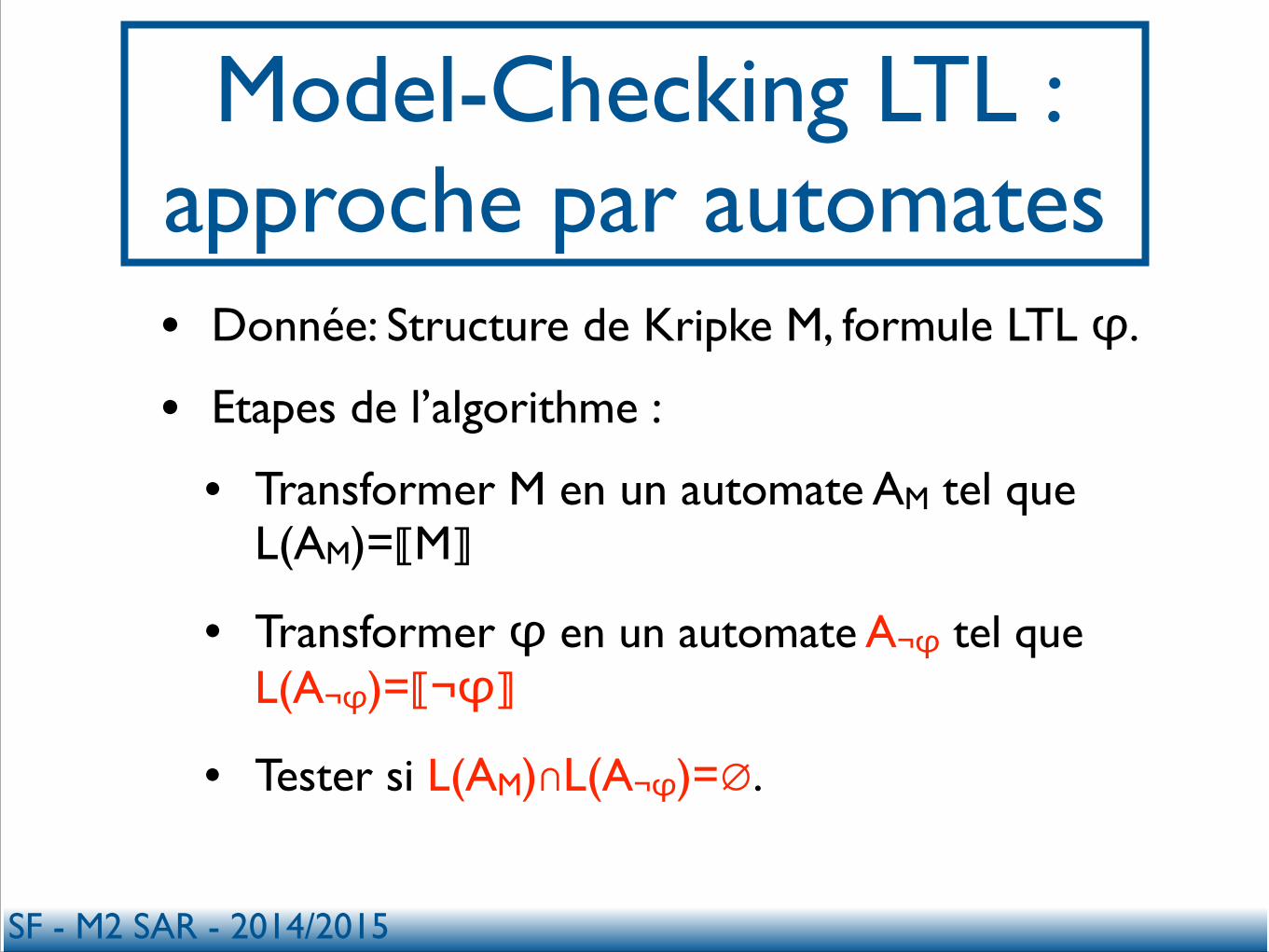
Model-Checking LTL : approche par automates• Donnée: Structure de Kripke M, formule LTL φ.
• Etapes de l’algorithme :
• Transformer M en un automate AM tel que L(AM)=⟦M⟧
• Transformer φ en un automate A¬φ tel que L(A¬φ)=⟦¬φ⟧ ✔
• Tester si L(AM)∩L(A¬φ)=∅.

SF - M2 SAR - 2014/2015
Model-Checking LTL : approche par automates• Donnée: Structure de Kripke M, formule LTL φ.
• Etapes de l’algorithme :
• Transformer M en un automate AM tel que L(AM)=⟦M⟧
• Transformer φ en un automate A¬φ tel que L(A¬φ)=⟦¬φ⟧ ✔
• Tester si L(AM)∩L(A¬φ)=∅.

SF - M2 SAR - 2014/2015
Transformer M en un automate de Büchi
• Soit M=(Q,T, A, q0, AP, l) une structure de Kripke. On construit un automate de Büchi B= (Q’, Σ, q’0, T’, F) tel que L(B)=⟦M⟧:
• Idée: on fait «basculer» les étiquettes des états vers les transitions + tous les états sont acceptants
• Σ=2AP
• Q’=T U {q0’}
• F=Q’
• Soit t=(q0,q)∈T, alors (q0’,l(q0),t)∈T’
• Soient t=(q,q’) et t’=(q’,q’’)∈T, alors (t,l(q’),t’)∈T’

SF - M2 SAR - 2014/2015
Exemple
• au tableau

SF - M2 SAR - 2014/2015
Model-Checking LTL : approche par automates• Donnée: Structure de Kripke M, formule LTL φ.
• Etapes de l’algorithme :
• Transformer M en un automate AM tel que L(AM)=⟦M⟧ ✔
• Transformer φ en un automate A¬φ tel que L(A¬φ)=⟦¬φ⟧ ✔
• Tester si L(AM)∩L(A¬φ)=∅.

SF - M2 SAR - 2014/2015
Model-Checking LTL : approche par automates• Donnée: Structure de Kripke M, formule LTL φ.
• Etapes de l’algorithme :
• Transformer M en un automate AM tel que L(AM)=⟦M⟧ ✔
• Transformer φ en un automate A¬φ tel que L(A¬φ)=⟦¬φ⟧ ✔
• Tester si L(AM)∩L(A¬φ)=∅.

SF - M2 SAR - 2014/2015
Tester le vide de l’intersection
• Construire l’automate AM⊗A¬φ tel que L(AM⊗A¬φ)= L(AM)∩L(A¬φ). (cf théorème)
• Rechercher s’il existe un mot accepté par AM⊗A¬φ . (cf théorème)

SF - M2 SAR - 2014/2015
Model-Checking LTL: catching bugs with a lasso

SF - M2 SAR - 2014/2015
Model-Checking LTL : approche par automates• Donnée: Structure de Kripke M, formule LTL φ.
• Etapes de l’algorithme :
• Transformer M en un automate AM tel que L(AM)=⟦M⟧ ✔
• Transformer φ en un automate A¬φ tel que L(A¬φ)=⟦¬φ⟧ ✔
• Tester si L(AM)∩L(A¬φ)=∅. ✔

SF - M2 SAR - 2014/2015
Model-Checking LTL : approche par automates• Donnée: Structure de Kripke M, formule LTL φ.
• Etapes de l’algorithme :
• Transformer M en un automate AM tel que L(AM)=⟦M⟧ ✔
• Transformer φ en un automate A¬φ tel que L(A¬φ)=⟦¬φ⟧ ✔
• Tester si L(AM)∩L(A¬φ)=∅. ✔
O(|M|)

SF - M2 SAR - 2014/2015
Model-Checking LTL : approche par automates• Donnée: Structure de Kripke M, formule LTL φ.
• Etapes de l’algorithme :
• Transformer M en un automate AM tel que L(AM)=⟦M⟧ ✔
• Transformer φ en un automate A¬φ tel que L(A¬φ)=⟦¬φ⟧ ✔
• Tester si L(AM)∩L(A¬φ)=∅. ✔
O(|M|)
O(2|φ|)

SF - M2 SAR - 2014/2015
Model-Checking LTL : approche par automates• Donnée: Structure de Kripke M, formule LTL φ.
• Etapes de l’algorithme :
• Transformer M en un automate AM tel que L(AM)=⟦M⟧ ✔
• Transformer φ en un automate A¬φ tel que L(A¬φ)=⟦¬φ⟧ ✔
• Tester si L(AM)∩L(A¬φ)=∅. ✔
O(|M|)
O(2|φ|)
O(|M|.2|φ|)

SF - M2 SAR - 2014/2015
Model-Checking LTL: techniques à la volée
• Pas nécessaire de construire l’automate produit en entier
• On construit pas à pas, et on s’arrête lorsqu’on trouve un cycle (=contre-exemple).

VFSR - M2 SAR - 2013/2014
Rappels de CTL

SF - M2 SAR - 2014/2015
CTL: syntaxe et sémantique
p
q,r p
r,s p,q q s
s ⊧ p ssi p∈l(s)

SF - M2 SAR - 2014/2015
CTL: syntaxe et sémantique
s ⊧ EXφ ssi il existe s’, successeur de s t.q. s’ ⊧φ
EXφ
φ

SF - M2 SAR - 2014/2015
CTL: syntaxe et sémantique
s ⊧ AXφ ssi pour tout s’, successeur de s, s’ ⊧φ
AXφ
φφ

SF - M2 SAR - 2014/2015
CTL: syntaxe et sémantique
s ⊧ EφUφ’ ssi il existe une exécution s0s1...sk telle que s0=s, sk ⊧φ’ et
pour tout 0≤i<k, si ⊧φ.
EφUφ’
φ
φ
φ’

SF - M2 SAR - 2014/2015
CTL: syntaxe et sémantique
s ⊧ AφUφ’ ssi pour toute exécution s0s1... telle que s0=s, ∃k t.q. sk
⊧φ’ et pour tout 0≤i<k, si ⊧φ.
AφUφ’
φφ
φ’
φ’
φ’
φ

SF - M2 SAR - 2014/2015
CTL: syntaxe et sémantique
φ::= p∈AP | ¬φ | φ∨φ |EXφ| AXφ| EφUφ | AφUφ
s ⊧ p ssi p∈l(s) s ⊧ ¬φ ssi s ⊭ φ s ⊧ φ1∨φ2 ssi s ⊧ φ1 ou s ⊧ φ2 s ⊧ EXφ ssi il existe s’, successeur de s, t.q. s’⊧φ s ⊧ AXφ ssi s’, pour tout s’, successeur de s, s’⊧φ s ⊧ Eφ1Uφ2 ssi il existe une exécution s0s1...sk tel que s0=s, sk ⊧φ2 et pour tout 0≤i≤k, si ⊧φ1. s ⊧ Aφ1Uφ2 ssi pour toute exécution s0s1... telle que s0=s, il existe k t.q. sk ⊧φ2 et pour tout 0≤i≤k, si ⊧φ1.
SF - M2 SAR - 2014/2015
CTL : macros
• EFφ ≣ E⊤Uφ
• AFφ≣A⊤Uφ
• EGφ≣¬AF¬φ
• AGφ≣¬EF¬φ

SF - M2 SAR - 2014/2015
CTL : Equivalences de formules
• AXφ=¬EX¬φ
• AφUφ’=¬E¬(φUφ’)=¬EG¬φ’∧¬E(¬φ’U(¬φ∧¬φ’))
SF - M2 SAR - 2014/2015
CTL : Lois d’expansion• AφUφ’=φ’∨(φ∧AX(AφUφ’))
• AFφ=φ∨(AXAFφ)
• AGφ=φ∧AXAGφ
• EφUφ’=φ’∨(φ∧EXE(φUφ’))
• EFφ=φ∨EXEFφ
• EGφ=φ∧EXEGφ
SF - M2 SAR - 2014/2015
CTL : lois distributives
• AG(φ∧φ’)=AGφ∧AGφ’
• EF(φ∨φ’)=EFφ∨EFφ’

SF - M2 SAR - 2014/2015
• Données : Une structure de Kripke M=(Q,T, A, Q0, AP, l) et une formule CTL φ.
• Question : Est-ce que M ⊧ φ?
• M ⊧ φ ssi Q0 ⊆S(φ).
Model-Checking de CTL

SF - M2 SAR - 2014/2015
Exercice
Exercises 433
6.11 Exercises
Exercise 6.1. Consider the following transition system over AP = { b, g, r, y }:
4
{ r }
{ y }{ g }
{ b }
1 2 3
The following atomic propositions are used: r (red), y (yellow), g (green), and b (black). Themodel is intended to describe a traffic light that is able to blink yellow. You are requested toindicate for each of the following CTL formulae the set of states for which these formulae hold:
(a) ∀♦ y (g) ∃" ¬ g
(b) ∀" y (h) ∀(b U ¬ b)
(c) ∀" ∀♦ y (i) ∃(b U ¬ b)
(d) ∀♦ g (j) ∀(¬ b U∃♦ b)
(e) ∃♦ g (k) ∀(g U ∀(y U r))
(f) ∃" g (l) ∀(¬ b U b)
Exercise 6.2. Consider the following CTL formulae and the transition system TS outlined onthe right:
Φ1 = ∀(a U b) ∨ ∃⃝ (∀" b)
Φ2 = ∀" ∀(a U b)
Φ3 = (a ∧ b) → ∃" ∃⃝ ∀(b W a)
Φ4 = (∀" ∃♦Φ3)
s0
∅s4
{ b }
s1
{ a }s2
{ a, b }s3
{ b }Determine the satisfaction sets Sat(Φi) and decide whether TS |= Φi (1 # i # 4).
Exercise 6.3. Which of the following assertions are correct? Provide a proof or a counterexample.
(a) If s |= ∃" a, then s |= ∀" a.
(b) If s |= ∀" a, then s |= ∃" a.
(c) If s |= ∀♦ a ∨ ∀♦ b, then s |= ∀♦ (a ∨ b).
(d) If s |= ∀♦ (a ∨ b), then s |= ∀♦ a ∨ ∀♦ b.
φ = A(aUb)∨EXEGb
φ=AG(A(aUb))
M⊧φ?

SF - M2 SAR - 2014/2015
Model-Checking de CTL : principe
• Procédure de marquage des états par les sous-formules de φ.
• Induction sur les sous-formules
• Arbre syntaxique de φ

SF - M2 SAR - 2014/2015
Arbre syntaxique : exemple
φ=EXa∧E(bU(EG¬c)) ∧
EX EU
a b EG
¬
c
SF - M2 SAR - 2014/2015
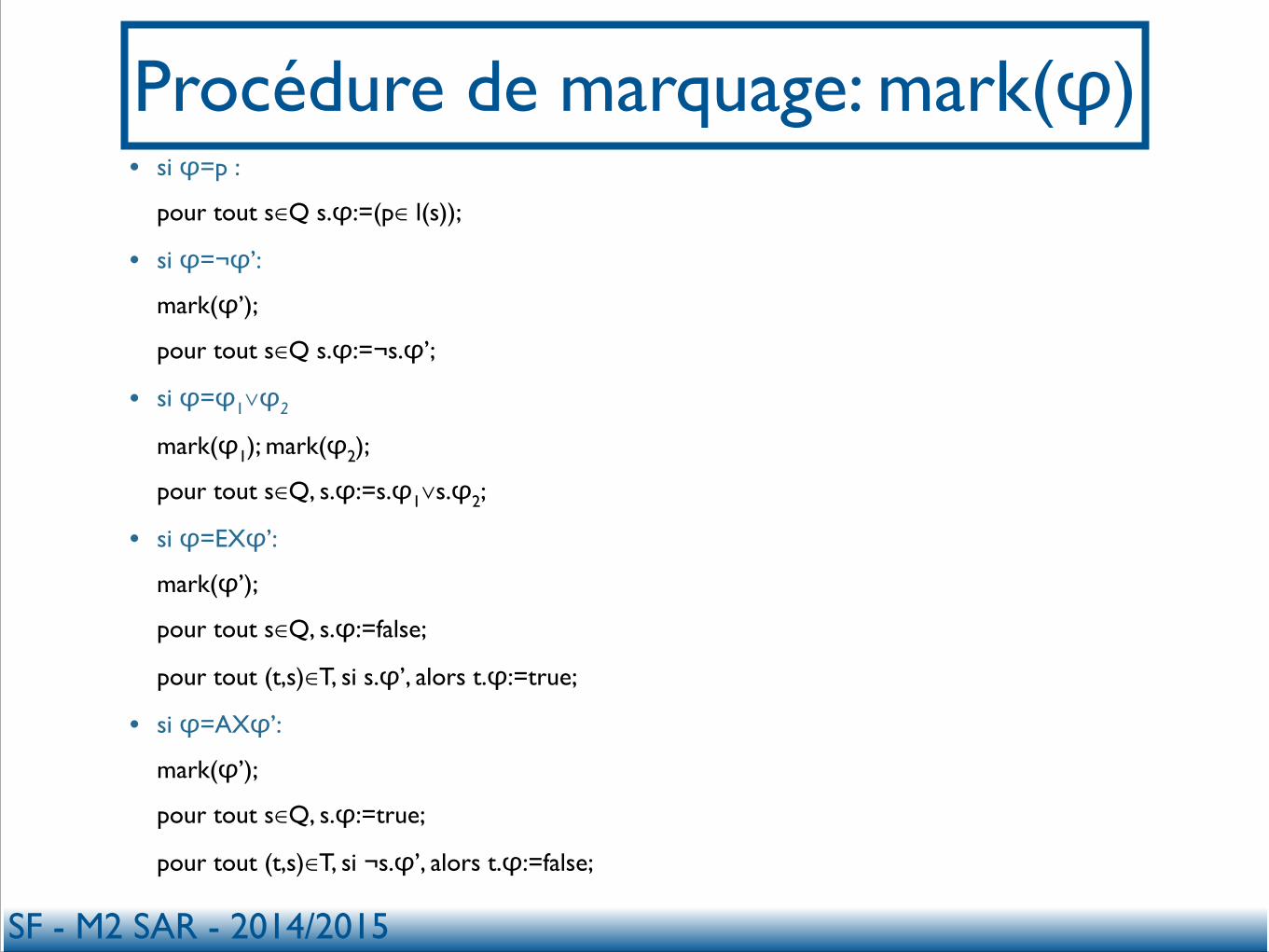
Procédure de marquage: mark(φ)• si φ=p :
pour tout s∈Q s.φ:=(p∈ l(s));
• si φ=¬φ’:
mark(φ’);
pour tout s∈Q s.φ:=¬s.φ’;
• si φ=φ1∨φ2
mark(φ1); mark(φ2);
pour tout s∈Q, s.φ:=s.φ1∨s.φ2;
• si φ=EXφ’:
mark(φ’);
pour tout s∈Q, s.φ:=false;
pour tout (t,s)∈T, si s.φ’, alors t.φ:=true;
• si φ=AXφ’:
mark(φ’);
pour tout s∈Q, s.φ:=true;
pour tout (t,s)∈T, si ¬s.φ’, alors t.φ:=false;

SF - M2 SAR - 2014/2015
Procédure de marquage: mark(φ)• cas Eφ1Uφ2: idée = Eφ1Uφ2≣φ2∨(φ1∧EX(Eφ1Uφ2))
X=Sat(φ2)U (Sat(φ1)∩Pre(X))
• si φ=Eφ1Uφ2 :
mark(φ1);mark(φ2);
L:=∅;
pour tout s∈Q, s.φ:=s.φ2; si s.φ, L:=L U{s};
tant que L≠∅
pour tout s∈L, L:=L∖{s};
pour tout prédécesseur t de s, si t. φ1∧¬t. φ, alors t. φ:=true ; L:=LU{t};

SF - M2 SAR - 2014/2015
Procédure de marquage: mark(φ)• cas Aφ1Uφ2: idée = Aφ1Uφ2≣φ2∨(φ1∧AX(Aφ1Uφ2))
X=Sat(φ2)U (Sat(φ1)∩{t∈S|∀s, (t,s)∈T, s∈X})
• si φ=Aφ1Uφ2 :
mark(φ1);mark(φ2);
L:=∅;
pour tout s∈Q, s.φ:=s.φ2; s.nb=degree(s);si s.φ, L:=L U{s};
tant que L≠∅
pour tout s∈L, L:=L∖{s};
pour tout prédécesseur t de s,
t.nb:=t.nb-1;
si t.nb:=0∧t. φ1∧¬t. φ, alors t. φ:=true ; L:=LU{t};

SF - M2 SAR - 2014/2015
Exemple : un four à microondes
[Model-Checking, Clarke, Grumberg, Peled]
StartError
CloseCloseHeat
StartCloseError
StartClose
StartCloseHeat
start oven
close door
close door
open door
start oven
open door
done
cook
open doorreset
warmup
start cooking
4
φ =AG(Start→AF Heat) =¬E(⊤U (Start∧¬(A(⊤U Heat))))
Start
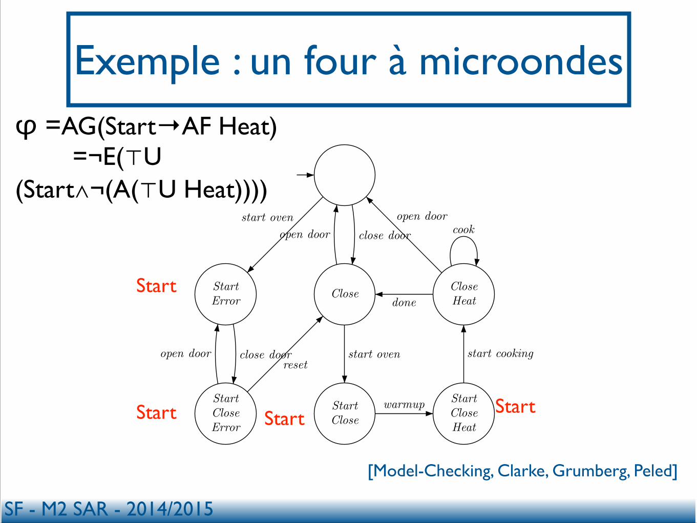
Start
Start
StartStart

SF - M2 SAR - 2014/2015
Exemple : un four à microondes
[Model-Checking, Clarke, Grumberg, Peled]
StartError
CloseCloseHeat
StartCloseError
StartClose
StartCloseHeat
start oven
close door
close door
open door
start oven
open door
done
cook
open doorreset
warmup
start cooking
4
φ =AG(Start→AF Heat) =¬E(⊤U (Start∧¬(A(⊤U Heat))))
Start
Start
Start
StartStartHeat
Heat

SF - M2 SAR - 2014/2015
Exemple : un four à microondes
[Model-Checking, Clarke, Grumberg, Peled]
StartError
CloseCloseHeat
StartCloseError
StartClose
StartCloseHeat
start oven
close door
close door
open door
start oven
open door
done
cook
open doorreset
warmup
start cooking
4
φ =AG(Start→AF Heat) =¬E(⊤U (Start∧¬(A(⊤U Heat))))
Start
Start
Start
StartStartHeat
HeatA(TUHeat)
A(TUHeat)
nb=2
nb=1
nb=2
nb=2
nb=3
nb=2 nb=1 nb=1

SF - M2 SAR - 2014/2015
Exemple : un four à microondes
[Model-Checking, Clarke, Grumberg, Peled]
StartError
CloseCloseHeat
StartCloseError
StartClose
StartCloseHeat
start oven
close door
close door
open door
start oven
open door
done
cook
open doorreset
warmup
start cooking
4
φ =AG(Start→AF Heat) =¬E(⊤U (Start∧¬(A(⊤U Heat))))
Start
Start
Start
StartStartHeat
HeatA(TUHeat)
A(TUHeat)
nb=2
nb=1
nb=2
nb=2
nb=2 nb=1 nb=1
nb=2

SF - M2 SAR - 2014/2015
Exemple : un four à microondes
[Model-Checking, Clarke, Grumberg, Peled]
StartError
CloseCloseHeat
StartCloseError
StartClose
StartCloseHeat
start oven
close door
close door
open door
start oven
open door
done
cook
open doorreset
warmup
start cooking
4
φ =AG(Start→AF Heat) =¬E(⊤U (Start∧¬(A(⊤U Heat))))
Start
Start
Start
StartStartHeat
HeatA(TUHeat)
A(TUHeat)
nb=2
nb=1
nb=2
nb=2
nb=2 nb=1
nb=2
nb=0

SF - M2 SAR - 2014/2015
Exemple : un four à microondes
[Model-Checking, Clarke, Grumberg, Peled]
StartError
CloseCloseHeat
StartCloseError
StartClose
StartCloseHeat
start oven
close door
close door
open door
start oven
open door
done
cook
open doorreset
warmup
start cooking
4
φ =AG(Start→AF Heat) =¬E(⊤U (Start∧¬(A(⊤U Heat))))
Start
Start
Start
StartStartHeat
HeatA(TUHeat)
A(TUHeat)
nb=2
nb=1
nb=2
nb=2
nb=2
nb=2
nb=0nb=0
A(TUHeat)

SF - M2 SAR - 2014/2015
Exemple : un four à microondes
[Model-Checking, Clarke, Grumberg, Peled]
StartError
CloseCloseHeat
StartCloseError
StartClose
StartCloseHeat
start oven
close door
close door
open door
start oven
open door
done
cook
open doorreset
warmup
start cooking
4
φ =AG(Start→AF Heat) =¬E(⊤U (Start∧¬(A(⊤U Heat))))
Start
Start
Start
StartStartHeat
HeatA(TUHeat)
A(TUHeat)
nb=2
nb=1
nb=2
nb=2
nb=2
nb=0nb=0
A(TUHeat)
nb=1

SF - M2 SAR - 2014/2015
Exemple : un four à microondes
[Model-Checking, Clarke, Grumberg, Peled]
StartError
CloseCloseHeat
StartCloseError
StartClose
StartCloseHeat
start oven
close door
close door
open door
start oven
open door
done
cook
open doorreset
warmup
start cooking
4
φ =AG(Start→AF Heat) =¬E(⊤U (Start∧¬(A(⊤U Heat))))
Start
Start
Start
StartStartHeat
HeatA(TUHeat)
A(TUHeat)nb=2 A(TUHeat)

SF - M2 SAR - 2014/2015
Exemple : un four à microondes
[Model-Checking, Clarke, Grumberg, Peled]
StartError
CloseCloseHeat
StartCloseError
StartClose
StartCloseHeat
start oven
close door
close door
open door
start oven
open door
done
cook
open doorreset
warmup
start cooking
4
φ =AG(Start→AF Heat) =¬E(⊤U (Start∧¬(A(⊤U Heat))))
Start
Start
Start
StartStartHeat
Heat
nb=2
¬A(TUHeat)
¬A(TUHeat)
¬A(TUHeat)
¬A(TUHeat)¬A(TUHeat)
¬A(TUHeat)

SF - M2 SAR - 2014/2015
Exemple : un four à microondes
[Model-Checking, Clarke, Grumberg, Peled]
StartError
CloseCloseHeat
StartCloseError
StartClose
StartCloseHeat
start oven
close door
close door
open door
start oven
open door
done
cook
open doorreset
warmup
start cooking
4
φ =AG(Start→AF Heat) =¬E(⊤U (Start∧¬(A(⊤U Heat))))
Start
Start
Start
nb=2
¬A(TUHeat)
¬A(TUHeat)
¬A(TUHeat)¬A(TUHeat)

SF - M2 SAR - 2014/2015
Exemple : un four à microondes
[Model-Checking, Clarke, Grumberg, Peled]
StartError
CloseCloseHeat
StartCloseError
StartClose
StartCloseHeat
start oven
close door
close door
open door
start oven
open door
done
cook
open doorreset
warmup
start cooking
4
φ =AG(Start→AF Heat) =¬E(⊤U (Start∧¬(A(⊤U Heat))))
Start
nb=2
¬A(TUHeat)¬A(TUHeat)
E(TUf)
E(TUf)
E(TUf)
E(TUf)
E(TUf)
E(TUf)
E(TUf)

SF - M2 SAR - 2014/2015
Exemple : un four à microondes
[Model-Checking, Clarke, Grumberg, Peled]
StartError
CloseCloseHeat
StartCloseError
StartClose
StartCloseHeat
start oven
close door
close door
open door
start oven
open door
done
cook
open doorreset
warmup
start cooking
4
φ =AG(Start→AF Heat) =¬E(⊤U (Start∧¬(A(⊤U Heat))))
Start
nb=2
¬A(TUHeat)¬A(TUHeat)
S(φ)=∅

SF - M2 SAR - 2014/2015
Complexité
• Complexité en temps est O(|M|.|φ|)
• MAIS formules CTL peuvent être plus grosses que formules LTL!

SF - M2 SAR - 2014/2015
Exercice350 Computation Tree Logic
{ a, b }s1s2
s3
s4 s5
s6 s7
{ a, b, c }
{ b, c }
{ b }
{ c } ∅
{ a }
{ a, c }
s0
Figure 6.11: An example of a transition system.
(a) (b)
(d)(c)
Figure 6.12: Example of backward search for ∃(trueU (a=c)∧ (a=b)).

VFSR - M2 SAR - 2013/2014
3.3 Inclure des notions d’équité
SF - M2 SAR - 2014/2015
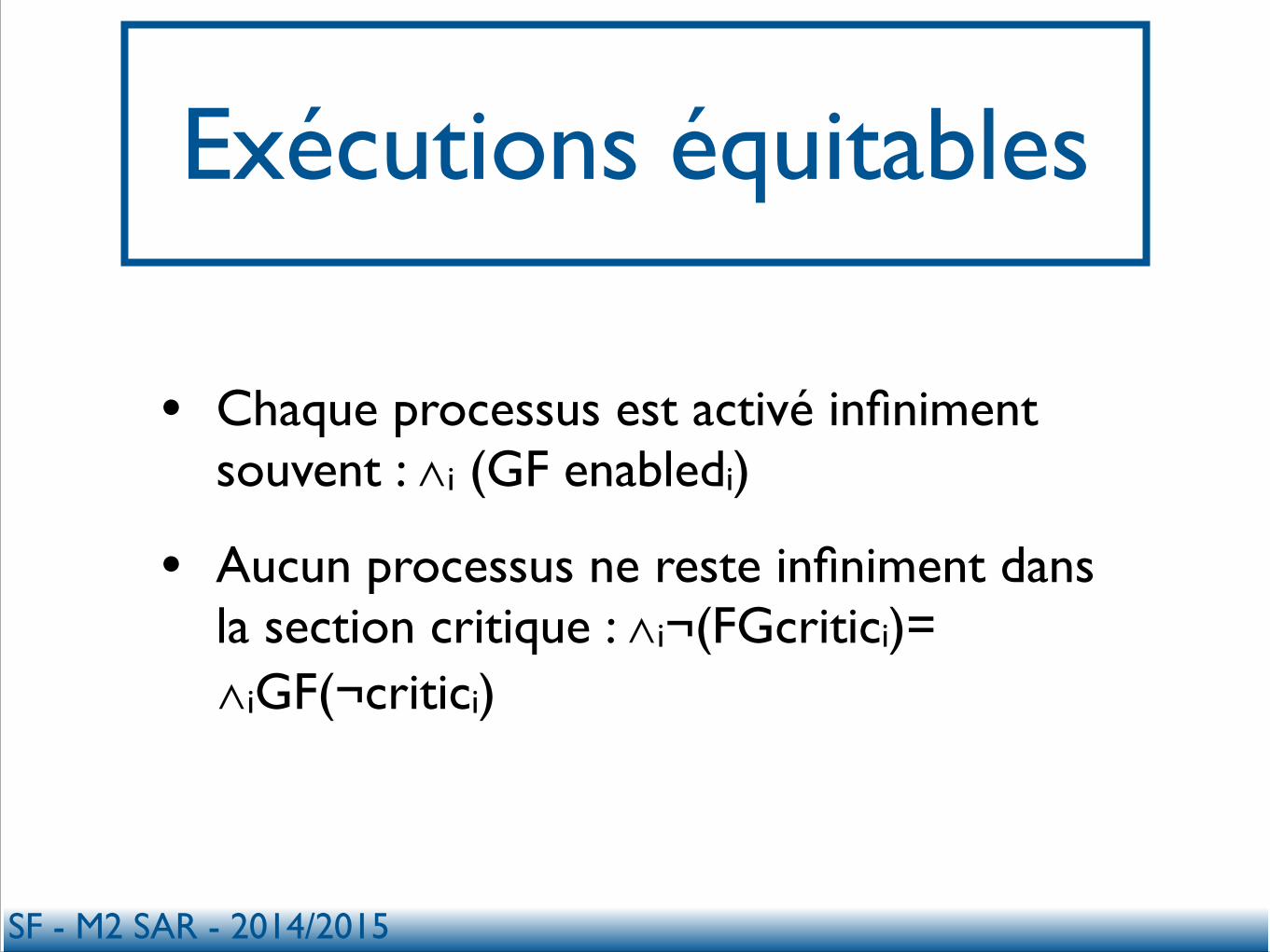
Exécutions équitables
• Chaque processus est activé infiniment souvent : ∧i (GF enabledi)
• Aucun processus ne reste infiniment dans la section critique : ∧i¬(FGcritici)= ∧iGF(¬critici)

SF - M2 SAR - 2014/2015
Contraintes d’équité
• Contrainte d’équité inconditionnelle : GFφ
• Contrainte d’équité forte : GFφ→GFφ’
• Contrainte d’équité faible : FGφ→GFφ’

SF - M2 SAR - 2014/2015
Conditions d’équité
• Une condition d’équité est une conjonction de contraintes d’équité
• Une condition d’équité est une formule LTL!

SF - M2 SAR - 2014/2015
Exécutions équitables
• Soit t une trace d’exécution d’une structure de Kripke M, fair une condition d’équité
• t est équitable si t,0⊧ fair

SF - M2 SAR - 2014/2015
LTL équitable
• Soit une structure de Kripke M, fair une condition d’équité et φ une formule LTL.
• M⊧ fair φ ssi t,0⊧ fair φ pour toute trace initiale t de M ssi t,0⊧ φ pour toute trace initiale équitable de M.

SF - M2 SAR - 2014/2015
ExempleParallelism and Communication 45
⟨n1, n2, y=1⟩
⟨w1, n2, y=1⟩ ⟨n1, w2, y=1⟩
⟨c1, n2, y=0⟩ ⟨w1, w2, y=1⟩ ⟨n1, c2, y=0⟩
⟨c1, w2, y=0⟩ ⟨w1, c2, y=0⟩
Figure 2.8: Mutual exclusion with semaphore (transition system representation).
first-in first-out (FIFO), or some other scheduling discipline can be chosen. Alternatively,another (more concrete) mutual exclusion algorithm could be selected that resolves thisscheduling issue explicitly. A prominent example of such algorithm has been provided in1981 by Peterson [332].
Example 2.25. Peterson’s Mutual Exclusion Algorithm
Consider the processes P1 and P2 with the shared variables b1, b2, and x. b1 and b2 areBoolean variables, while x can take either the value 1 or 2, i.e., dom(x) = { 1, 2 }. Thescheduling strategy is realized using x as follows. If both processes want to enter thecritical section (i.e., they are in location waiti), the value of variable x decides which ofthe two processes may enter its critical section: if x = i, then Pi may enter its criticalsection (for i = 1, 2). On entering location wait1, process P1 performs x := 2, thus givingprivilege to process P2 to enter the critical section. The value of x thus indicates whichprocess has its turn to enter the critical section. Symmetrically, P2 sets x to 1 whenstarting to wait. The variables bi provide information about the current location of Pi.More precisely,
bi = waiti ∨ criti .
bi is set when Pi starts to wait. In pseudocode, P1 performs as follows (the code for processP2 is similar):

SF - M2 SAR - 2014/2015
ExempleParallelism and Communication 45
⟨n1, n2, y=1⟩
⟨w1, n2, y=1⟩ ⟨n1, w2, y=1⟩
⟨c1, n2, y=0⟩ ⟨w1, w2, y=1⟩ ⟨n1, c2, y=0⟩
⟨c1, w2, y=0⟩ ⟨w1, c2, y=0⟩
Figure 2.8: Mutual exclusion with semaphore (transition system representation).
first-in first-out (FIFO), or some other scheduling discipline can be chosen. Alternatively,another (more concrete) mutual exclusion algorithm could be selected that resolves thisscheduling issue explicitly. A prominent example of such algorithm has been provided in1981 by Peterson [332].
Example 2.25. Peterson’s Mutual Exclusion Algorithm
Consider the processes P1 and P2 with the shared variables b1, b2, and x. b1 and b2 areBoolean variables, while x can take either the value 1 or 2, i.e., dom(x) = { 1, 2 }. Thescheduling strategy is realized using x as follows. If both processes want to enter thecritical section (i.e., they are in location waiti), the value of variable x decides which ofthe two processes may enter its critical section: if x = i, then Pi may enter its criticalsection (for i = 1, 2). On entering location wait1, process P1 performs x := 2, thus givingprivilege to process P2 to enter the critical section. The value of x thus indicates whichprocess has its turn to enter the critical section. Symmetrically, P2 sets x to 1 whenstarting to wait. The variables bi provide information about the current location of Pi.More precisely,
bi = waiti ∨ criti .
bi is set when Pi starts to wait. In pseudocode, P1 performs as follows (the code for processP2 is similar):
GF(w1∧¬c2)→GFc1∧GF(w2∧¬c1)→GFc2
∧
(FGn1→GFw1)∧(FGn2→GFw2)
M⊧fair GFc1∧GFc2

SF - M2 SAR - 2014/2015
Model-Checking LTL équitable
Théorème : M⊧fair φ ssi M⊧ fair → φ.

SF - M2 SAR - 2014/2015
CTL équitable
• Conditions d’équité ne peuvent pas s’écrire en CTL
• On voudrait dire A(fair→φ) ou E(fair∧φ)
mais ce sont des formules CTL*

SF - M2 SAR - 2014/2015
CTL équitable
φ::= p∈AP | ¬φ | φ∨φ |EfXφ| AfXφ| EfφUφ | AfφUφ
s ⊧ p ssi p∈l(s) s ⊧ ¬φ ssi s ⊭ φ s ⊧ φ1∨φ2 ssi s ⊧ φ1 ou s ⊧ φ2 s ⊧ EfXφ ssi il existe une exécution équitable s0s1... tel que s0=s, t.q. s1⊧φ s ⊧ AfXφ ssi s’, pour toute exécution équitable s0s1... telle que s0=s, s1⊧φ s ⊧ Efφ1Uφ2 ssi il existe une exécution équitable s0s1...sk tel que s0=s, sk ⊧φ2 et pour tout 0≤i≤k, si ⊧φ1. s ⊧ Afφ1Uφ2 ssi pour toute exécution équitable s0s1... telle que s0=s, il existe k t.q. sk ⊧φ2 et pour tout 0≤i≤k, si ⊧φ1.

SF - M2 SAR - 2014/2015
Model-Checking de CTL équitable
• On suppose qu’on a étiqueté les états avec une nouvelle AP fair, qui indique s’il existe une exécution équitable partant de l’état
• s⊧EfXφ ssi s⊧EX(φ∧fair)
• s⊧AfXφ ssi s⊧AX(¬fair∨φ)
• s⊧EfφUφ’ ssi s⊧EφU(fair∧φ’)
• s⊧AfφUφ’ ssi s⊧¬EfG¬φ’∧¬Ef(¬φ’U(¬φ∧¬φ’)) ssi s⊧¬EfG¬φ’∧¬E(¬φ’U(fair∧¬φ∧¬φ’))

SF - M2 SAR - 2014/2015
Model-Checking de CTL équitable
• 1er problème : Comment calculer fair?
• Rappel : s⊧fair ssi il existe une exécution équitable partant de s
• → Dépend de la condition d’équité!
• 2ème problème : calculer EfGφ

SF - M2 SAR - 2014/2015
Calculer fair : les composantes fortement connexes
Définition : Dans un graphe, une composante fortement connexe (SCC) est un sous-graphe maximal tel que pour toute paire de noeuds (s,s’) s’ est accessible depuis s, et s est accessible depuis s’
L’algorithme de Tarjan permet de calculer les SCC d’un graphe en temps linéaire.

SF - M2 SAR - 2014/2015
Calculer fair : le cas inconditionnel
• On considère une condition d’équité de la forme ∧iGFφi, avec φi formule CTL.
• On marque les états par les φi.
• On calcule les SCC de M par l’algorithme de Tarjan.
• Soit S’ l’union des SCC qui intersecte S(φi), pour tout i.
• fair est l’ensemble des états pouvant atteindre S’.
• (accessibilité se calcule en temps linéaire)

SF - M2 SAR - 2014/2015
Calculer EfGφ : le cas inconditionnel
• Effectuer mark(φ).
• Soit M(φ) la restriction de M aux états de S(φ).
• Calculer les SCC de M(φ) (algo de Tarjan).
• Soit S’ l’union de SCC de M(φ) intersectant S(φi), pour tout i.
• M,s⊧EfGφ ssi M,s⊧EφUS’ ssi M(φ),s⊧EFS’.
• →problème d’accessibilité.
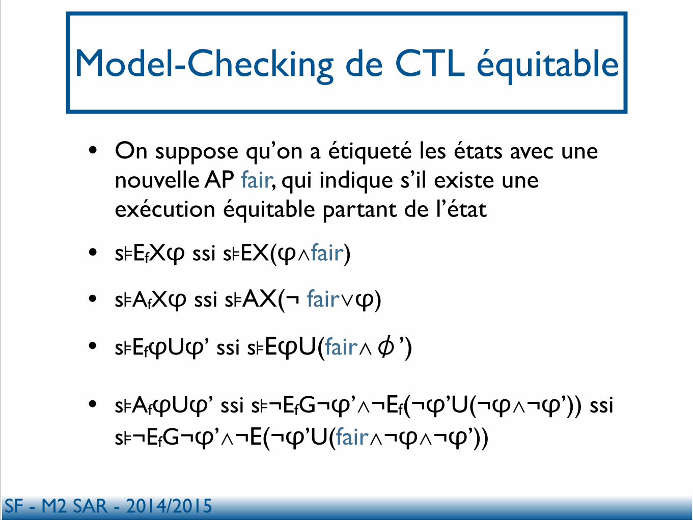
SF - M2 SAR - 2014/2015
Model-Checking de CTL équitable
• On suppose qu’on a étiqueté les états avec une nouvelle AP fair, qui indique s’il existe une exécution équitable partant de l’état
• s⊧EfXφ ssi s⊧EX(φ∧fair)
• s⊧AfXφ ssi s⊧AX(¬ fair∨φ)
• s⊧EfφUφ’ ssi s⊧EφU(fair∧φ’)
• s⊧AfφUφ’ ssi s⊧¬EfG¬φ’∧¬Ef(¬φ’U(¬φ∧¬φ’)) ssi s⊧¬EfG¬φ’∧¬E(¬φ’U(fair∧¬φ∧¬φ’))

SF - M2 SAR - 2014/2015
Model-Checking de CTL équitable
• On suppose qu’on a étiqueté les états avec une nouvelle AP fair, qui indique s’il existe une exécution équitable partant de l’état
• s⊧EfXφ ssi s⊧EX(φ∧fair)
• s⊧AfXφ ssi s⊧AX(¬ fair∨φ)
• s⊧EfφUφ’ ssi s⊧EφU(fair∧φ’)
• s⊧AfφUφ’ ssi s⊧¬EfG¬φ’∧¬Ef(¬φ’U(¬φ∧¬φ’)) ssi s⊧¬EfG¬φ’∧¬E(¬φ’U(fair∧¬φ∧¬φ’))
✔
✔

SF - M2 SAR - 2014/2015
Et aussi...
• Autres logiques temporelles : CTL*,mu-calcul... (plus expressives), ForSpec, PSL, Sugar... (industrie)
• Méthodes efficaces : méthodes symboliques, techniques de réduction (ordres partiels...)
Recommended