No. 655 / September 2019
Loan to value caps and government-backed mortgage insurance: Loan-level evidence from Dutch residential mortgages
Leo de Haan and Mauro Mastrogiacomo
De Nederlandsche Bank NV
P.O. Box 98
1000 AB AMSTERDAM
The Netherlands
Working Paper No. 655
September 2019
Loan to value caps and government-backed mortgage insurance: Loan-level evidence from Dutch residential mortgages Leo de Haan and Mauro Mastrogiacomo *
* Views expressed are those of the author and do not necessarily reflect official positions of
De Nederlandsche Bank.

1
Loan to value caps and government-backed mortgage insurance:
Loan-level evidence from Dutch residential mortgages
Leo de Haan ab and Mauro Mastrogiacomo acd
a De Nederlandsche Bank b Centrale Bank van Aruba
c Vrij Universiteit Amsterdam d Netspar
September 2019
Abstract
Using loan level data on mortgage loans originated by Dutch banks during 1996 to 2015, we
analyse the determinants of the incidence of non-performance. We find that both the originating
loan-to-value ratio (OLTV) and the debt-service-to-income ratio (DSTI) are significantly
positively associated with the probability of non-performance. The results suggest that
mortgages with government-loan-guarantees perform better. Moreover, several mortgage loan
and borrower characteristics, such as the (interest-only) loan type and the underwater status of
the borrower, increase credit risk. Our model predictions suggest a novel policy implication: in
order to avoid acceleration of non-performance probabilities, the OLTV-limit should be set to
about 70%-80% for uninsured mortgages, and to about 90% for those with mortgage insurance.
JEL classification: G20, G21, H81
Keywords: Credit risk, Mortgage loans, Loan to Value, Loan guarantees
We thank Dennis Olson, Conor O’Toole, and participants of the DNB seminar (May, 2019) and the World
Finance Conference (July, 2019) for useful comments and advice. The views expressed are those of the authors
and do not necessarily reflect the positions of DNB or CBA. Corresponding author. Email: [email protected]
2
1. Introduction
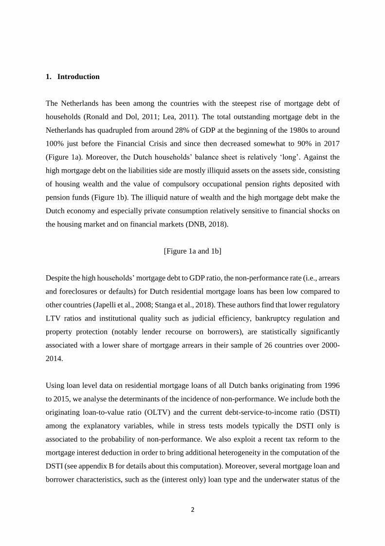
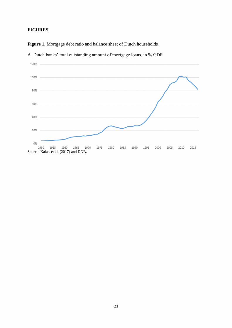
The Netherlands has been among the countries with the steepest rise of mortgage debt of
households (Ronald and Dol, 2011; Lea, 2011). The total outstanding mortgage debt in the
Netherlands has quadrupled from around 28% of GDP at the beginning of the 1980s to around
100% just before the Financial Crisis and since then decreased somewhat to 90% in 2017
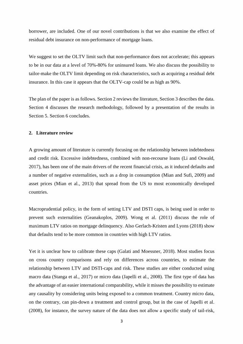
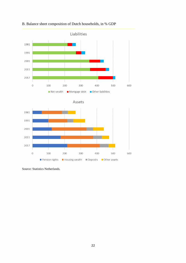
(Figure 1a). Moreover, the Dutch households’ balance sheet is relatively ‘long’. Against the
high mortgage debt on the liabilities side are mostly illiquid assets on the assets side, consisting
of housing wealth and the value of compulsory occupational pension rights deposited with
pension funds (Figure 1b). The illiquid nature of wealth and the high mortgage debt make the
Dutch economy and especially private consumption relatively sensitive to financial shocks on
the housing market and on financial markets (DNB, 2018).
[Figure 1a and 1b]
Despite the high households’ mortgage debt to GDP ratio, the non-performance rate (i.e., arrears
and foreclosures or defaults) for Dutch residential mortgage loans has been low compared to
other countries (Japelli et al., 2008; Stanga et al., 2018). These authors find that lower regulatory
LTV ratios and institutional quality such as judicial efficiency, bankruptcy regulation and
property protection (notably lender recourse on borrowers), are statistically significantly
associated with a lower share of mortgage arrears in their sample of 26 countries over 2000-
2014.
Using loan level data on residential mortgage loans of all Dutch banks originating from 1996
to 2015, we analyse the determinants of the incidence of non-performance. We include both the
originating loan-to-value ratio (OLTV) and the current debt-service-to-income ratio (DSTI)
among the explanatory variables, while in stress tests models typically the DSTI only is
associated to the probability of non-performance. We also exploit a recent tax reform to the
mortgage interest deduction in order to bring additional heterogeneity in the computation of the
DSTI (see appendix B for details about this computation). Moreover, several mortgage loan and
borrower characteristics, such as the (interest only) loan type and the underwater status of the
3
borrower, are included. One of our novel contributions is that we also examine the effect of
residual debt insurance on non-performance of mortgage loans.
We suggest to set the OLTV limit such that non-performance does not accelerate; this appears
to be in our data at a level of 70%-80% for uninsured loans. We also discuss the possibility to
tailor-make the OLTV limit depending on risk characteristics, such as acquiring a residual debt
insurance. In this case it appears that the OLTV-cap could be as high as 90%.
The plan of the paper is as follows. Section 2 reviews the literature, Section 3 describes the data.
Section 4 discusses the research methodology, followed by a presentation of the results in
Section 5. Section 6 concludes.
2. Literature review
A growing amount of literature is currently focusing on the relationship between indebtedness
and credit risk. Excessive indebtedness, combined with non-recourse loans (Li and Oswald,
2017), has been one of the main drivers of the recent financial crisis, as it induced defaults and
a number of negative externalities, such as a drop in consumption (Mian and Sufi, 2009) and
asset prices (Mian et al., 2013) that spread from the US to most economically developed
countries.
Macroprudential policy, in the form of setting LTV and DSTI caps, is being used in order to
prevent such externalities (Geanakoplos, 2009). Wong et al. (2011) discuss the role of
maximum LTV ratios on mortgage delinquency. Also Gerlach-Kristen and Lyons (2018) show
that defaults tend to be more common in countries with high LTV ratios.
Yet it is unclear how to calibrate these caps (Galati and Moessner, 2018). Most studies focus
on cross country comparisons and rely on differences across countries, to estimate the
relationship between LTV and DSTI-caps and risk. These studies are either conducted using
macro data (Stanga et al., 2017) or micro data (Japelli et al., 2008). The first type of data has
the advantage of an easier international comparability, while it misses the possibility to estimate
any causality by considering units being exposed to a common treatment. Country micro data,
on the contrary, can pin-down a treatment and control group, but in the case of Japelli et al.
(2008), for instance, the survey nature of the data does not allow a specific study of tail-risk,
4
which is a problem as defaults in several countries occur in less than 3% of the relevant
population.
In this sense, replacing survey data with supervisory micro data would be a better choice, as the
tail risks are better represented. Evidently such data are not easily suited for international
comparisons. Kelly and O’Toole (2019) use a double trigger default model to identify
thresholds effects showing that Buy-to-Let mortgage loan defaults increase with the OLTV ratio
and fall with the originating debt service ratio measured as rental value to instalment at
origination. This is the only study we have found that investigates the issue using loan level
data. Specifically, they use 2014 Q4 Buy-to-Let loan level data of Irish banks headquartered in
the UK, representing 2 percent of the UK mortgage market.
Finally, when macroprudential limits are exceeded, the institutional setting becomes relevant
for the onset of possible market failures. In a non-recourse system, the effect of macroprudential
instruments is limited by moral hazard, for instance in the case of strategic defaults (Guiso et
al., 2013). In a full recourse system instead, a similar limitation could arise in the presence of
mortgage insurance (Kim et al, 2018).
We extend on previous studies by using a dataset for the Netherlands that contains 1.5 million
or about 90% of the residential mortgage loans underwritten by the Dutch banking sector. This
highly representative sample has the advantage of allowing identification of specific subgroups,
and to focus on tail events, such as arrears and defaults or foreclosures, that are barely observed
in survey data.1 The Dutch data provide a unique opportunity to investigate the effect on the
rate of non-performance of government backed residual mortgage debt insurance. This
insurance is called a Nationale Hypotheek Garantie (NHG). As noted by Lea (2011), the
mortgage insurer is a government-owned fund, the so-called Homeownership Guarantee Fund
(in Dutch: Waarborgfonds Eigen Woning). The fund is a private institution with fall-back
agreements with the national and municipal governments. These agreements form the basis for
interest-free loans to the Fund from the national and municipal governments at times when its
assets are no longer sufficient to meet claims. This means that the Fund is able to comply with
its payment obligations at all times. As a result, the Dutch central bank (in Dutch: De
Nederlandsche Bank (DNB)) considers the NHG as a government guarantee. According to the
1 For example, the ECHP survey data used by Japelli et al. (2008) include only 5000 Dutch mortgage loans.
5
figures shown by Lea (2011), mortgage default rates in the Netherlands are among the lowest
internationally. This raises the question whether the low default rate is related to the NHG. Debt
insurance may have significant effects. For example, De Haan (2003) finds that NHG affects
monetary transmission, in the sense that a bank lending channel is operative in the Netherlands
but only for unsecured lending and not for secured lending, possibly because loans with NHG
get special treatment by banks.
3. Data
De Nederlandsche Bank (DNB) started in 2012 the collection of the DNB loan level data (LLD).
This initiative is based on the RMBS template used by the European Central Bank (ECB),
within the framework of their 100% transparency policy on securitized loans, available through
the European Data Warehouse (EDW). The LLD is an extension of the ECB data. The EDW
version of the data only contains securitized loans, a minor fraction of (typically) low-risk loans.
The LLD used in this paper instead also includes the back-books of banks, with their entire
stock of loans.
Coverage of the LLD and comparability with other sources is high (Mastrogiacomo and Van
der Molen, 2015). The data contains about 80% of all loans of Dutch households, and more than
90% of those issued by Dutch banks to residents. The composition by banks is given in Table
1.
[Table 1]
The data are reported on quarterly basis by the main 12 Dutch banks, and the collection started
in the fourth quarter of 2012. Each wave contains about 6 million loans, issued to 3 million
borrowers. This means that on average every Dutch borrower combines at least 2 loans.
We use the 2016Q2 wave of the LLD. Relevant to this paper are several indicators, such as the
originating Loan to Value ratio (OLTV), i.e. the LTV ratio at origination of the loan, and
household income at origination of the loan, which we use to compute the current mortgage
debt service to income ratio (DSTI), the loan type (interest-only or not), and the status of each
loan (performing or non-performing, i.e. in arrear or foreclosed).
6
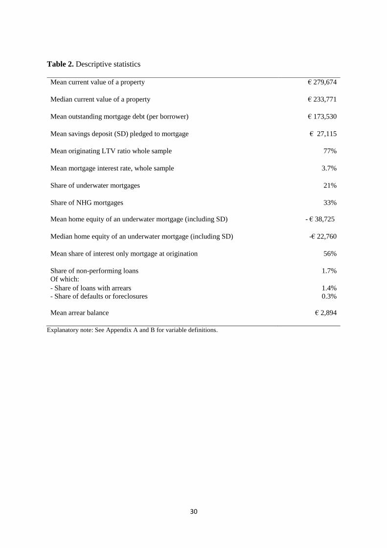
Table 2 summarizes some relevant mortgage characteristics that are elicited using the LLD. The
table shows several indicators revealing the main features of the Dutch mortgage market. In the
LLD, it is for instance possible to elicit the value of the saving deposits pledged to the mortgage.
This means that the mean outstanding debt is a net concept, as these deposits have been
subtracted. This is important to keep in mind, because technically these deposits are pledged in
order to provide full redemption only at maturity. However, in the LLD, these are treated as
per-period amortizations. Further the table shows the OLTV for the whole stock. Due to
expanding monetary policy, the interest rate for an insured loan with a 10 years reset period (the
most common product in the Netherlands) has dropped from about 4% to less than 2%, however
it will take time before this reduction is spread to all households, that is why the mean interest
rate presented here is higher. This is possibly due to several mitigants that protect households
from interest rate fluctuations. It is very important to have information about the loan level
interest rate, as we use it to compute the DSTI (see Appendix B). With the reduction of the
interest rate, also reset-periods have become on average longer and have now passed the 10
years mark. Finally, the table shows the reduction in risk elicited by several other
characteristics, such as the share of underwater mortgages, of interest only loans, and of non-
performing loans and their balances.
[Table 2]
The data also allows zooming into two specific features of the Dutch mortgage market. First,
upon purchasing a house with a value below a legislated threshold, new home-owners can insure
their loan against the risk of residual debt. This insurance, as mentioned in Section 2, is called
a Nationale Hypotheekgarantie (NHG). A default is not strictly needed for the insurance to be
activated. Those selling a property with an underwater mortgage, can apply for reimbursement
of residual debt. The NHG will then reimburse the bank and become the sole creditor of the
mortgage owner. If specific conditions are met, the NHG will pardon debt fully if the mortgage
was amortizing and partially if not. The specific conditions to qualify for pardoning depend on
the reason for selling the house. If this was necessary due to unemployment, disability, death of
a partner or divorce, NHG will pardon. Since 2014 also an affordability test can be carried out
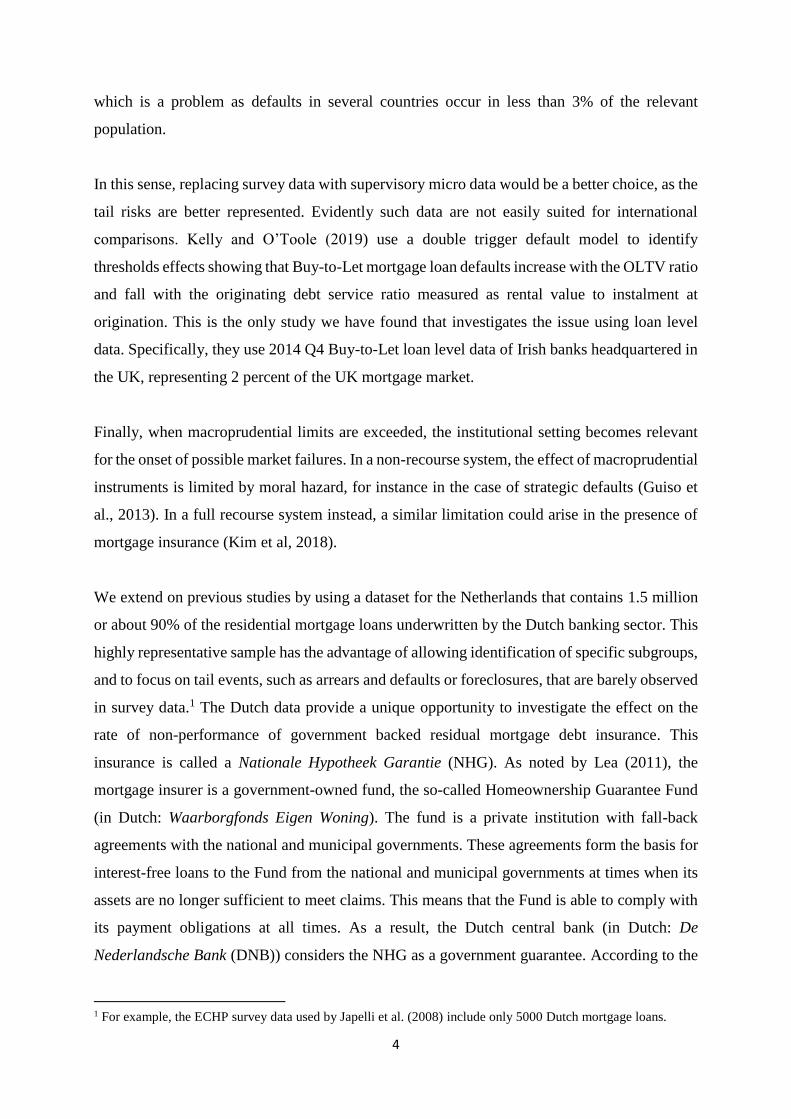
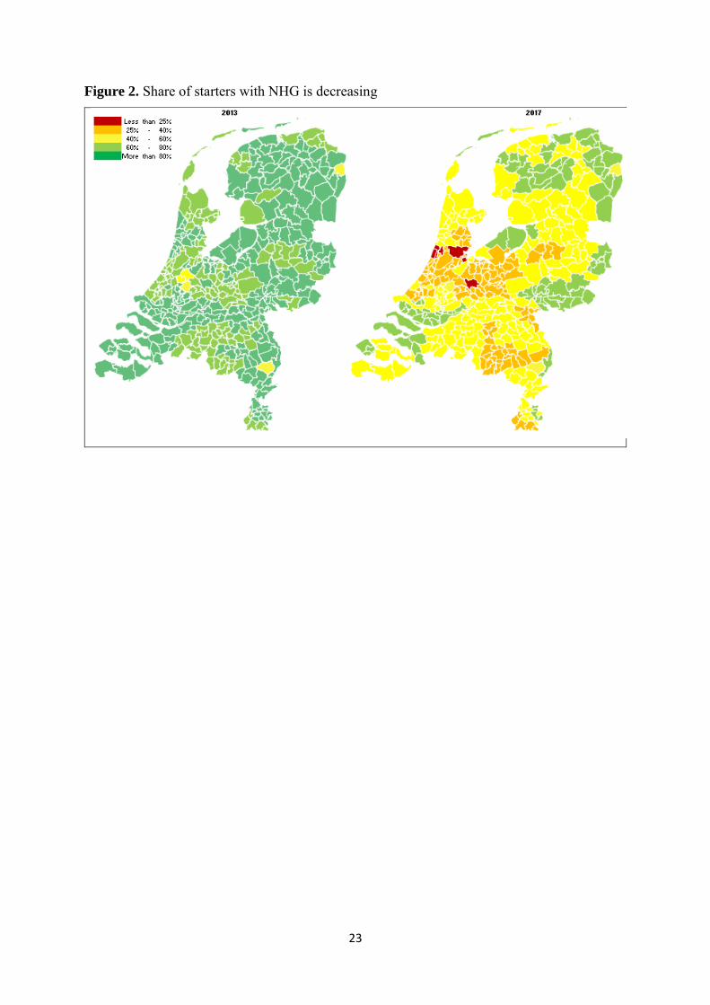
in specific cases. Figure 2 shows that participation in this scheme has been historically very
popular among starters, but that recently this has reduced in the whole country (due to increasing

7
prices, mostly in large municipalities such as Amsterdam, and decreasing qualification
thresholds). In our sample, 33% of loans have an NHG.
[Figure 2]
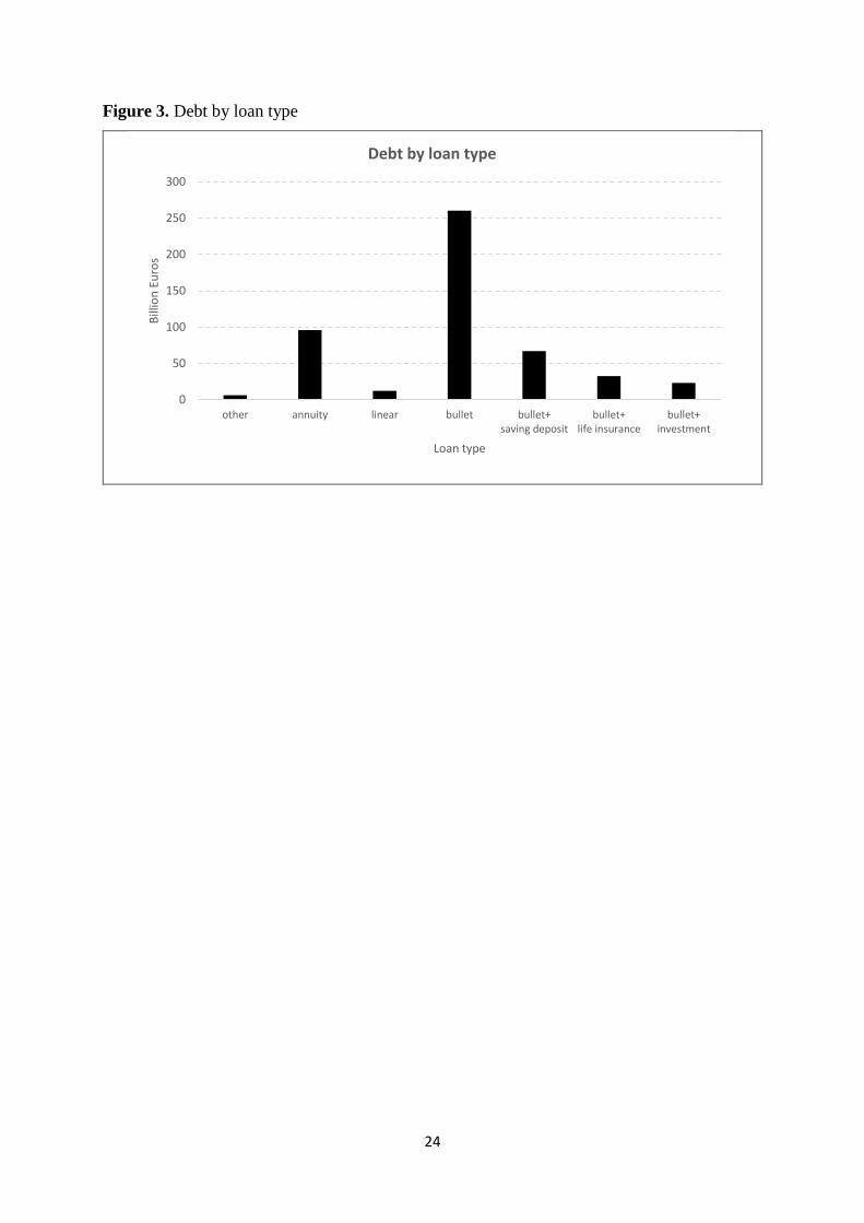
Second, in the past 20 years, many interest-only (or so-called ‘bullet’) loans have been sold.
Figure 3 shows that more than 55% of loans outstanding are of such type, and thus do not
contractually amortize. The LLD also allows calculating the share of interest-only loans
applicable to each borrower. It appears that only one third of the borrowers has a fully interest-
only loan, while about half combines such loans with (semi) amortizing loans. The group of
fully interest-only borrowers has somewhat lower outstanding debt, is older and has used the
mortgage more often for home-equity extraction (Mastrogiacomo and van der Molen, 2015).
[Figure 3]
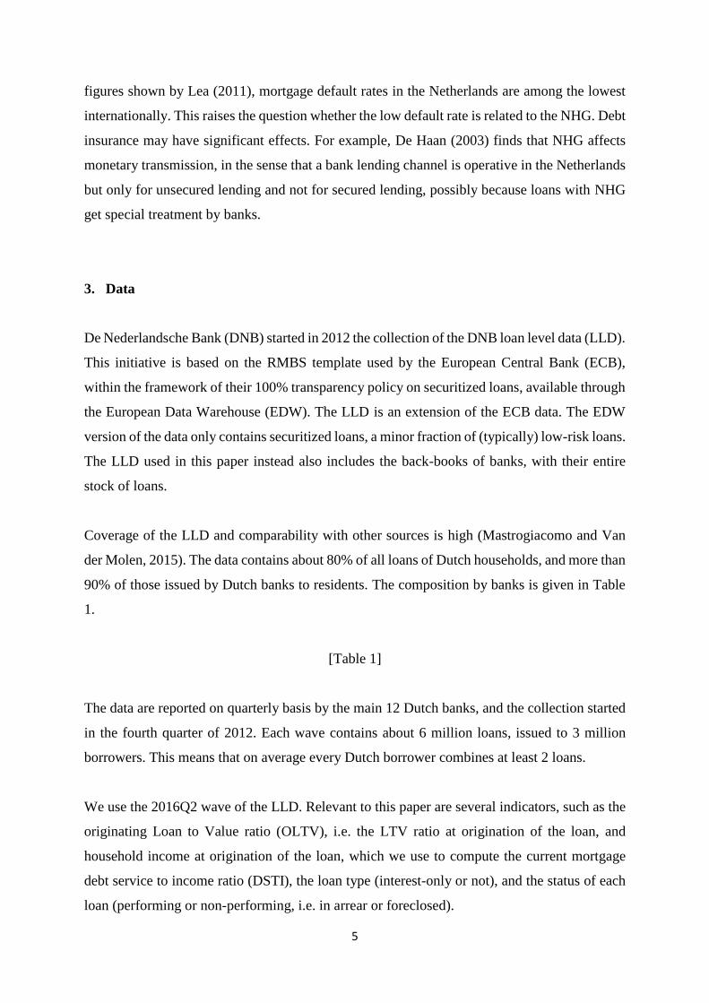
We define a mortgage as non-performing (NP) if there is an arrear or a foreclosure or default
in any of the underlying loans. Figure 4 shows the NP rate for NHG-loans and non-NHG
loans, by year of loan origination. The NP rate of non-NHG loans increased from 0.9% in
1996 to 2.4% in the global financial crisis year 2008 and subsequently decreased to 0.6% in
2015.
Figure 4 also shows that the NP rate of non-NHG participants before the crisis was in some
years significantly higher than the dashed line for NHG participants. The two lines cross after
2009. After the crisis, NHG-loans defaulted more often. Two possible explanations could be
given for this evidence. Kim et al (2018) discuss the possibility of moral hazard, as the
insurance reduces the consequences of a default for the insured. This would in principle lift
the dashed line up. But also changes in institutions could be partly responsible. In 2010 NHG
requirements (such as comply with LTI rules) became compulsory also for non-NHG loans,
thus reducing their risk. This second effect could lower the solid line.
[Figure 4]

8
4. Methodology
In this section, we first introduce the potential determinants of the probability to non-perform
that we will test in the empirical model. Next, we present our empirical model of the probability
to non-perform. In order to treat all observations consistently, we arrange the data at borrower
level. So, the borrower is our unit of analysis. This is an obvious choice, as the main triggers in
our model, OLTV and DSTI, are not defined at loan level. We thus use the detailed loan level
information to construct the following variables at borrower level.
4.1 Determinants of non-performing status
1. The originating Loan to Value ratio (OLTV) at origination of the mortgage is defined
as the sum of all principals of all loans of a borrower divided by the value of the house.
Kelly and O’Toole (2019), using loan level data for buy-to-let mortgages, find that the
greater the size of a mortgage in relation to the value of the house at the time of the
origination of the loan, the higher is the probability of a future NP. Typically, stress-test
models assume that LTV ratios only affect loss given default (LGD), but when
mortgages are underwater defaults may increase (for instance due to strategic defaults;
see, e.g., Ampudia et al., 2014).
2. The mortgage debt service to income ratio (DSTI) is defined as all payment obligations
of the loans owned by a borrower divided by the borrower’s income. This is partly
affected by recent tax reforms that add heterogeneity across groups and will help the
identification of the effect. For the definition of DSTI we refer to Appendix B. We
expect a positive association between this variable and non-performance.
3. NHG is a binary indicator of the presence of residual debt insurance, as discussed in
Section 3. This is equal to 1 if a borrower insures any of his loans against the risk of
residual debt upon selling the house. The borrower pays a lump-sum-fee to the
foundation when taking the loan (in 2016 this is 1%). On the other hand, lenders grant
to borrowers with insurance a discount on the mortgage interest rate (between 0.3 and
0.6 percent point). The insurance can be obtained for loans up to a maximum amount (€
245.000 in 2016). The insurance can be bought only by borrowers with a proportion of

9
income which is spent on housing below a certain limit2: hence, the insurance signals
that there is a solid income base for the debt service. Also defaulting or foreclosing is
not strictly necessary to obtain a reimbursement, as also a downsizer qualifies. Our
assumption therefore is that the presence of NHG diminishes the risk of becoming non-
performing.
4. The age of the loan-applicant in years is assumed to have a negative relationship with
non-performance as older borrowers, being more advanced on their financial life cycle,
often are wealthier and more credit worthy than younger ones. They are also survivors
in the data, thus more likely to not default.
5. Underwater status of the mortgage (or, so-called ‘negative equity’) is a binary indicator
telling whether the outstanding principal of all loans of a borrower is greater or not than
the current value of the house. Households facing the dual trigger of affordability
problems and negative equity are more likely to go into longer-term arrears (Gerlach-
Kristen and Lyons, 2018).
6. The self-employment status of the loan-applicant is a binary indicator telling whether
the borrower at the time of loan origination was self-employed or not. We assume that
self-employed are more at risk of income fluctuations and therefore loans to self-
employed run higher risk to not perform. 8% of loan applicants in the data are self-
employed.
7. The purpose of the loan is also assumed to affect the non-performing status. We look at
the purpose of a borrower’s largest loan if there are more than one loan. When the
mortgaged house is partly used for commercial purposes, credit risk is expected to be
higher, as one is more at risk of income fluctuations.
8. An interest-only loan is a loan without contractual amortization during the loan term.
We assume that interest-only loans have more credit-risk than loans which are repaid
during the loan term, as the former are more exposed to interest rate shocks. We use the
share of interest-only in the total mortgage debt of the borrower.
2 DSTI-caps (also called LTI-caps in the Netherlands as an annuity is always assumed) are comply-or-explain rules. This means that some exceptions are allowed and some borrowers can borrow more than the DSTI limit allows. However, NHG will not accept these borrowers as costumers. Only compliers are accepted. In the LLD we observe about 10% of non-compliers to the DSTI cap for the whole sample.
10
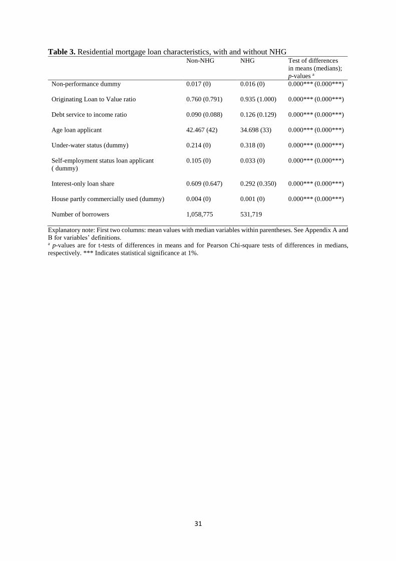
Table 3 gives the mean and median values of the explanatory variables for the 1,590,494
borrowers in the sample, split up according to whether their mortgage is insured by NHG or
not. From these summary statistics, some tentative inferences can be made. Loan applicants
with an NHG are relatively young, less often self-employed, and less frequently using their
house partly for commercial purposes. NHG holders have higher OLTV and DSTI ratios and
their houses are more often underwater. Nevertheless, their non-performance rate is comparable
or even somewhat lower (on average 1 percentage point) than that of their counterparts without
an NHG. Also, NHG holders use interest-only loans less often.
[Table 3]
4.2 Empirical model
We employ a logit model of the probability of a borrower to become non-performing. Non-
performing status NP can be 1 or 0 (either a case of default/arrear or not). The logit model
assumes that the probability of NP = 1 is a logistic function of the linear expression (𝛽0 + 𝛽1𝑥):
𝑝(𝑁𝑃 = 1) =1
1+𝑒−(𝛽0+𝛽1𝑥) = 𝐹(𝑥), (1)
where p(x) is the probability of non-performance NP = 1, given some linear combination of a
vector of predictors x, with e denoting the exponential function. As the value of the linear
expression can vary from negative to positive infinity, after transformation, the resulting
probability p(x) ranges between 0 and 1. β0 is the intercept from the linear equation, β1 a vector
of coefficients.
A logistic regression is performed to find the β parameters that best fit:
𝑁𝑃 = {10
𝐷′ = 𝛽0 + 𝛽1𝑥 + 𝜀 ≥ 0
𝐷′ = 𝛽0 + 𝛽1𝑥 + 𝜀 < 0
, (2)
where ε is an error distributed by the standard normal distribution in case of a probit model. The
associated latent variable is NP′ = 𝛽0 + 𝛽1𝑥 + 𝜀 where both NP’ and ε are unobserved, hence
11
‘latent’. We assume that among the predictors X are the loan-to-value ratio (OLTV), the debt-
service-to-income ratio (DSTI), and other control variables Z.
𝑝(𝑁𝑃 = 1) = 𝐹(𝐿𝑇𝑉𝑖, 𝐷𝑆𝑇𝐼𝑖, 𝑍𝑖) (3)
Our a-priori expectations are that both OLTV and DSTI positively affect the NP-probability.
Control variables Z contain borrower-specific or dwelling controls including borrower age,
applicant employment status, presence of a Dutch mortgage guarantee, binary indicator of
underwater status, purpose of the loan, loan type, as introduced in Section 4.1.
5. Results
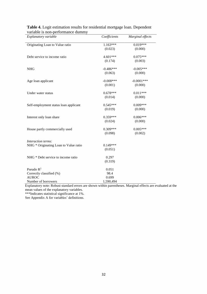
Table 4 gives the estimation results for the logit model relating the NP-status to the explanatory
variables introduced above. Two interaction terms have been added to the model, the first
interacting OLTV with NHG and the first interacting DSTI with NHG. The purpose of this
interaction is to examine differences between NHG and non-NHG holders with respect to the
determinants of non-performance.
[Table 4]
The first column gives the estimated coefficients, the magnitudes of which are not easy to
interpret in terms of probability effects. Therefore, for ease of interpretation, the marginal
effects of the explanatory variables are also given, being the partial derivatives of the probability
with respect to the explanatory variables evaluated at their respective means. The advantage of
marginal effects is that they are directly interpretable in terms of the implied effect of each
variable on the NP-probability.
5.1 OLTV, DSTI and NHG
The estimate of 0.019 for the marginal effect of the OLTV ratio means that if the OLTV ratio
is 0.1 (or 10 percentage points) higher, the NP-probability increases by 0.0019 (or 0.19
percentage point). This is both statistically significant and economically significant, as the mean
NP-rate is 1.7 percent. The marginal effect of the NHG dummy is -0.005, which means that
NHG loans on average run 0.5 percent lower risk of non-performance. Figure 5, panel A, depicts
12
the predicted non-performance probabilities for mortgage loans with and without NHG for
different OLTV ratios. The dotted lines denote 95% confidence intervals. The difference
between the two NP probability lines, around 0.005 or 0.5 percentage point, reflect the marginal
effect of the NHG, but the difference is greater (smaller) for higher (lower) OLTV ratios. This
means that NHG loans not only have lower NP-probabilities but that the sensitivity for higher
OLTVs is also somewhat smaller.
[Figure 5]
The marginal effect for the debt service to income ratio (DSTI) is 0.075 meaning that if the
DSTI ratio increases by 0.1 or 10 percentage points, the NP-probability increases by .0075 or
0.75 percentage point. Figure 5, panel B, also shows that the difference between the two lines
is around 0.005 or 0.5 percentage point, but greater (smaller) for higher (lower) DSTI ratios.
Hence, NHG loans not only have lower NP-probabilities but are also less sensitive to higher
DSTIs.
The shapes of the predicted NP-probability curves in Figure 5 are convex, which is typical for
exponential logit functions. The curves are smooth and have no kinks, because each explanatory
variable in the logistic regression equation has only one coefficient. An alternative approach,
which allows for varying coefficients for an explanatory variable, is to use a spline function
which fits a piecewise regression between specific points, known as knots, of the continuous
variable. Following a number of applications in the medical literature, Kelly and O’Toole
(2019) applied a restricted cubic spline in their analysis of defaults of UK buy-to-let loans. We
adopt their approach by also allowing for a non-linear relationship between the knots using the
restricted cubic spline. When using a restricted cubic spline, one obtains a continuous smooth
function that is linear before the first knot, a piecewise cubic polynomial between adjacent
knots, and linear again after the last knot. In general, the logit restricted cubic spline model,
with restricted spline function f(SV), with k knots is given by:
𝑝(𝑁𝑃 = 1) = 𝐹(𝐿𝑇𝑉𝑖, 𝐷𝑆𝑇𝐼𝑖, 𝑍𝑖 , 𝑓(𝑆𝑉)) (4)
with 𝑓(𝑆𝑉) = 𝛽0 + 𝛽1𝑆𝑉1 + 𝛽2𝑆𝑉2 + ⋯ + 𝛽𝑘−1𝑆𝑉𝑘−1 and the other variables as defined in Eq.
(3). SV represents the variable V upon which the spline function is applied. In our case, this
relates to two variables: OLTV and DSTI. We adapt the default five equally spaced percentiles
13
recommended by Harrell (2001), i.e., the knots are located at the 5, 27.5, 50, 72.5 and 95
percentiles of the distributions of OLTV and DSTI. This is in line with Kelly and O’Toole
(2019).
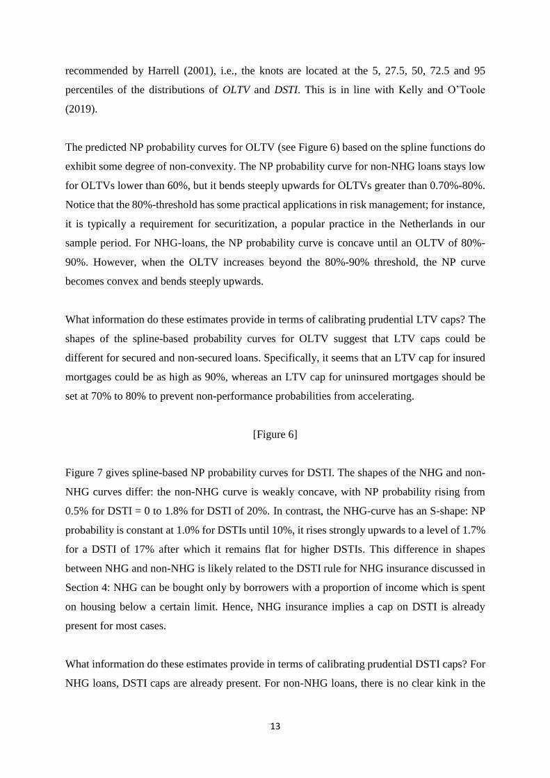
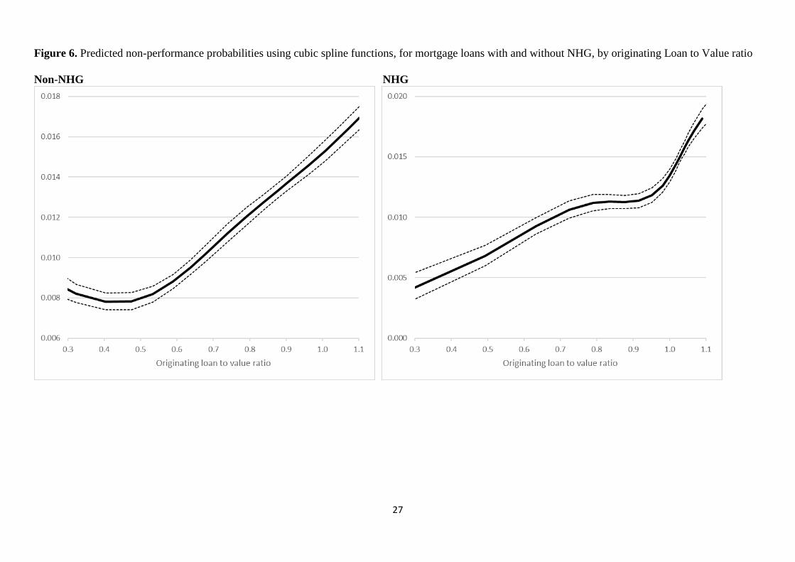
The predicted NP probability curves for OLTV (see Figure 6) based on the spline functions do
exhibit some degree of non-convexity. The NP probability curve for non-NHG loans stays low
for OLTVs lower than 60%, but it bends steeply upwards for OLTVs greater than 0.70%-80%.
Notice that the 80%-threshold has some practical applications in risk management; for instance,
it is typically a requirement for securitization, a popular practice in the Netherlands in our
sample period. For NHG-loans, the NP probability curve is concave until an OLTV of 80%-
90%. However, when the OLTV increases beyond the 80%-90% threshold, the NP curve
becomes convex and bends steeply upwards.
What information do these estimates provide in terms of calibrating prudential LTV caps? The
shapes of the spline-based probability curves for OLTV suggest that LTV caps could be
different for secured and non-secured loans. Specifically, it seems that an LTV cap for insured
mortgages could be as high as 90%, whereas an LTV cap for uninsured mortgages should be
set at 70% to 80% to prevent non-performance probabilities from accelerating.
[Figure 6]
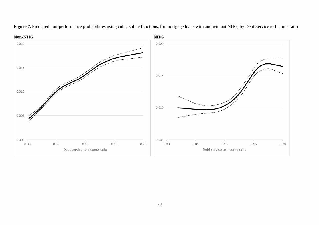
Figure 7 gives spline-based NP probability curves for DSTI. The shapes of the NHG and non-
NHG curves differ: the non-NHG curve is weakly concave, with NP probability rising from
0.5% for DSTI = 0 to 1.8% for DSTI of 20%. In contrast, the NHG-curve has an S-shape: NP
probability is constant at 1.0% for DSTIs until 10%, it rises strongly upwards to a level of 1.7%
for a DSTI of 17% after which it remains flat for higher DSTIs. This difference in shapes
between NHG and non-NHG is likely related to the DSTI rule for NHG insurance discussed in
Section 4: NHG can be bought only by borrowers with a proportion of income which is spent
on housing below a certain limit. Hence, NHG insurance implies a cap on DSTI is already
present for most cases.
What information do these estimates provide in terms of calibrating prudential DSTI caps? For
NHG loans, DSTI caps are already present. For non-NHG loans, there is no clear kink in the
14
NP probability curve which means there is no clear indication of where a DSTI cap could best
be calibrated.
[Figure 7]
5.2 Other explanatory variables
Older borrowers have lower credit risk. The marginal effect is small, however (-0.01 percentage
point per year). Borrowers whose houses are ‘under water’ run higher risk of non-performance.
The marginal effect is 1.1 percentage point. Borrowers who were self-employed when taking
on the loan, run higher risk of non-performance. The marginal effect is 0.9 percentage point.
Interest only loans have somewhat higher credit risk. The marginal effect of the interest only
loan share is 0.6. The purpose of the main loan is also a determining factor for credit risk. If
loans were mainly taken on houses that were partly commercially used, credit risk was 0.5
percentage point higher.
6. Conclusions
Using loan level data on residential mortgage loans originated by all Dutch banks during 1996
to 2015, we analyse the determinants of the incidence of non-performance, i.e., arrears or
defaults.
We find that both the originating loan-to-value ratio (OLTV) and the debt-service-to-income
ratio (DSTI) are significantly positively associated with the probability of mortgage arrears.
The results also suggest that mortgages with government backed debt insurance (NHG) perform
better. Moreover, several mortgage loan and borrower characteristics, such as the (interest only)
loan type and the underwater status of the borrower, increase credit risk. The age of the borrower
diminishes credit risk. The loan purpose is also a significant determinant: in case the financing
of a commercially used property, credit risk is higher.

15
The estimates also provide information in terms of calibrating prudential LTV caps. The shapes
of the spline-based probability curves for OLTV suggest that LTV caps could be different for
secured and non-secured loans. Specifically, it seems that an LTV cap for insured mortgages
could be as high as 90%, whereas an LTV cap for uninsured mortgages should be set at 70% to
80% to prevent non-performance probabilities from accelerating.

16
References
Ampudia, M., H. van Vlokhoven and D. Zochowski (2014), Financial fragility of euro area
households, ECB Working Paper No. 1737.
De Haan, L. (2003), Microdata evidence on the bank lending channel in the Netherlands, De
Economist 151(3), 293-315.
De Nederlandsche Bank (2018), Strong correlation between consumption and house prices in
the Netherlands, DNBulletin 25 January. https://www.dnb.nl/en/news/news-and-
archive/DNBulletin2018/dnb371605.jsp
Galati, G. and R. Moessner (2018), What do we know about the effects of macroprudential
policy? Economica 85(340), 735-770.
Geanakoplos, J. (2009), The Leverage Cycle, in: NBER Macroeconomics Annual 2009, volume
24, D. Acemoglu, K. Rogoff and M. Woodford (Eds.), University of Chicago Press, 1-65.
Gerlach-Kristen, P. and S. Lyons (2018), Determinants of mortgage arrears in Europe: evidence
from household microdata, International Journal of Housing Policy 18(4), 545-567.
Guiso, L., P. Sapienza and L. Zingales (2013), The determinants of attitudes toward strategic
default on mortgages , The Journal of Finance 68(4), 1473-1515.
Japelli, T., M. Pagano and M. di Maggio (2008), Households’ indebtedness and financial
fragility. Centre for Studies in Economics and Finance Working Paper No. 208.
Kakes, J, H. Loman and R. Van der Molen (2017), Verschuivingen in de financiering van
hypotheekschuld, Economische Statistische Berichten 102(4749S), 69-73.
Kelly, R. and C. O’Toole (2019), Mortgage default, lending conditions and macroprudential
policy: Loan-level evidence from UK buy-to-lets, Journal of Financial Stability 36, 322-335.
Kim, Y., M. Mastrogiacomo, S. Hochguertel and H. Bloemen (2018), Till debt do us part:
Strategic divorces, economic outcomes and a test of moral hazard, Netspar Industry Paper
forthcoming.
Lea, M. (2011), Alternative forms of mortgage finance: What can we learn from other
countries?, AREUEA Annual Conference paper.
Li, W. and F. Oswald (2017), Recourse and residential mortgages: The case of Nevada. Journal
of Urban Economics 101, 1–13
Mastrogiacomo, M. and R. van der Molen (2015), Dutch mortgages in the DNB loan level data,
DNB Occasional Study 4.
Mian, A. and A. Sufi (2009), The consequences of mortgage credit expansion: Evidence from
the U.S. mortgage default crisis, Quarterly Journal of Economics 124(4), 1449-1496.

17
Mian, A., K. Rao and A. Sufi (2013), Household balance sheets, consumption, and the economic
slump, Quarterly Journal of Economics 128(4), 1687–1726.
Ronald, R. and K. Dol (2011), Housing in the Netherlands before and after the global financial
crisis, in: R. Forrest and N.-M. Yip (eds.), Housing Markets and the Global Financial Crisis:
The Uneven Impact on Households. Edward Elgar.
Stanga, I., R. Vlahu and J. de Haan (2017), Mortgage arrears, regulation and institutions: Cross-
country evidence, DNB working paper 580.
Wong, E., T. Fong, K. Li and H. Choi (2011), Loan-to-value ratio as a macroprudential tool –
Hong Kong SAR’s experience and cross-country evidence. Hong Kong Monetary Authority
Working Paper 01/2011.

18
Appendix A: Variable definitions
The data collection of DNB is based on the ECB templates that is used for the European Data
Warehouse RMBS data. However, we have slightly modified some definitions in order to
guarantee consistency over time.
Variable Definition
Non-Performing (NP) Account status equal to default / foreclosure
or arrears. We take this indicator at collateral
level, so if only one of the loans linked to a
specific collateral is defaulted, we assume
that the borrower who owns that collateral is
in default.
Originating Loan to Value ratio Loan To Value ratio at origination of the
loan. For second line loans this is the
combined or total OLTV.
Debt service to income ratio See Appendix B
NHG Nationale Hypotheek Garantie, i.e. mortgage
debt insurance. Type of guarantee provider
being the Waarborgfonds Eigen Woning
Age loan applicant Age of main applicant.
Under water status A dummy equal to 1 if the current valuation
amount is larger than the current principal.
Definition net of pledged saving accounts,
when these are proxied using inception date
rather than origination date. We apply a 2%
haircut to the current valuation amount,
which is an indexed value relative to the
original valuation using local indexes
provided by Statistics Netherlands.
Self-employed status Self-employed status of the primary
applicant at origination.
Interest only loan This loan type is separately identified as
being a bullet loan. These loans do not
amortize and thus do not have a maturity
date. For borrowers with multiple loans, the
share of interest only in the total is used.
House partly commercially used A dummy equal to 1 if the house is (partly)
commercially used.

19
Appendix B: Assumptions made for calculation of debt service to income (DSTI) ratio
The DSTI ratio is not reported in the LLD template. We thus define a mortgage DSTI ratio that
only takes mortgage debt into account. We need to tackle two main challenges. First, periodic
payments are not well defined in the template and often only report the payments received by
the bank (typically only interest) and not the amortization or the savings deposits. Second,
income is only observed at origination. Below, a detailed explanation of how we deal with both
issues is given. The mortgage DSTI is then computed as being equal to the ratio between the
monthly total net periodic payments on all loan parts of the borrower, divided by the borrower’s
net monthly current income.
Periodic payments.
In order to have a clear indication of periodic payments, we must distinguish among the
different loan types. In the scheme below, we explain how we deal with each loan type. We
kept the notation simple, but some of the variables listed below contain more detailed
information. Specifically, the marginal tax rate for the mortgage interest deduction (tax) is
individual and time specific. This relevant because exogenous changes to tax policy have taken
place. From 2012 the marginal tax rate was progressively reduced in steps of 0.5% points to
borrowers with higher incomes. So, over time, the net period payments of these borrowers, have
increased, ceteris paribus. This reform has the advantage to bring additional heterogeneity into
the model.

20
Loan type Net periodic payment (NPP)
Interest only loan NPP = 𝑃 ∗ 𝑟 ∗ (1 − 𝑡𝑎𝑥)
Annuity or linear
loan
AP = (𝑟
1−(1+𝑟)−𝑙𝑒𝑛𝑔𝑡ℎ) ∗ 𝑃
AA = 𝐴𝑃 – 𝑃 ∗ 𝑟
NPP = 𝐴𝐴 + 𝑅𝑃 ∗ 𝑟 ∗ (1 − 𝑡𝑎𝑥)
Saving or life-
insurance loan SP =
𝑃
(1+𝑟)𝑙𝑒𝑛𝑔𝑡ℎ
1−((1+𝑟)−1)𝑙𝑒𝑛𝑔𝑡ℎ
1−((1+𝑟)−1)
NPP = 𝑆𝑃 + 𝑃 ∗ 𝑟 ∗ (1 − 𝑡𝑎𝑥)
Investment loan IP =
𝑃
(1+𝑘)𝑙𝑒𝑛𝑔𝑡ℎ
1−((1+𝑘)−1)𝑙𝑒𝑛𝑔𝑡ℎ
1−((1+𝑘)−1)
NPP = 𝐼𝑃 + 𝑃 ∗ 𝑟 ∗ (1 − 𝑡𝑎𝑥)
Legend: P = principal, r = interest rate on loan, tax = marginal tax rate of mortgage interest deduction, AP =
annuity premium, length = difference in years between maturity date and origination date, AA = annuity
amortization, RP = residual annuity debt after amortization, SP= Saving premium, IP = investment premium (how
much is transferred to investment fund each period), k = expected return from investment = 8% (this is the
maximum expected return that brokers could use according to tax law)
Current Income
In the LLD, we only observe income at loan origination. This is a household income, in the
sense banks either report the sum of the incomes of the borrowers (if they are a couple) or the
separate incomes of the two members of the couple. For the computation of the mortgage DSTI,
we need current income, but this is not observed. In order to proxy current income, we apply a
wage inflation to original income from the date of origination to the present day. This means
that all households receive the mean wage increase in each period. This is of course an
overestimation for those who might lose their jobs or decide to work part-time. At the same
time this could be an underestimation for those households where one starts working more or
experiences a promotion. These measurement errors might cancel out each other to some extent,
and become possibly more severe, the older the loan. In the LLD however, 50% of the loans
have originated in the last 7 years, due to the frequent resets.
The resulting DSTI is trimmed by deleting the 1st and 99th percentile of the distribution,
assuming that these extreme values are outliers that may be due to mismeasurement.
21
FIGURES
Figure 1. Mortgage debt ratio and balance sheet of Dutch households
A. Dutch banks’ total outstanding amount of mortgage loans, in % GDP
Source: Kakes et al. (2017) and DNB.
22
B. Balance sheet composition of Dutch households, in % GDP
Source: Statistics Netherlands.
23
Figure 2. Share of starters with NHG is decreasing
24
Figure 3. Debt by loan type
0
50
100
150
200
250
300
other annuity linear bullet bullet+saving deposit
bullet+life insurance
bullet+investment
Bill
ion
Eu
ros
Loan type
Debt by loan type

25
Figure 4. Non-performing rate for mortgage loan with and without NHG, by year of loan
origination
0,000
0,005
0,010
0,015
0,020
0,025
1996 1998 2000 2002 2004 2006 2008 2010 2012 2014
Non-NHG NHG

26
Figure 5. Predicted non-performance probabilities for mortgage loans with and without NHG, by originating Loan to Value and Debt Service to Income ratio
A. By originating Loan to Value B. By Debt Service to Income
0,000
0,005
0,010
0,015
0,020
0,025
0,030
0,00 0,05 0,10 0,15 0,20
Debt service to income ratio
NHG Non-NHG 95% confidence band
27
Figure 6. Predicted non-performance probabilities using cubic spline functions, for mortgage loans with and without NHG, by originating Loan to Value ratio
Non-NHG NHG
28
Figure 7. Predicted non-performance probabilities using cubic spline functions, for mortgage loans with and without NHG, by Debt Service to Income ratio
Non-NHG NHG

29
TABLES
Table 1. Sample composition, by underwriting bank
Bank Percentage
of number
of
borrowers
ABN Amro Bank 19.9
Achmea 3.1
Aegon 2.0
ING 32.8
NIBC 2.3
Nationale Nederlanden 1.4
Rabobank 38.3
Van Lanschot 0.2
Total 100.0
30
Table 2. Descriptive statistics
Mean current value of a property € 279,674
Median current value of a property
€ 233,771
Mean outstanding mortgage debt (per borrower)
€ 173,530
Mean savings deposit (SD) pledged to mortgage
€ 27,115
Mean originating LTV ratio whole sample
77%
Mean mortgage interest rate, whole sample
3.7%
Share of underwater mortgages
21%
Share of NHG mortgages 33%
Mean home equity of an underwater mortgage (including SD) - € 38,725
Median home equity of an underwater mortgage (including SD)
-€ 22,760
Mean share of interest only mortgage at origination
56%
Share of non-performing loans 1.7% Of which: - Share of loans with arrears 1.4% - Share of defaults or foreclosures
0.3%
Mean arrear balance € 2,894
Explanatory note: See Appendix A and B for variable definitions.
31
Table 3. Residential mortgage loan characteristics, with and without NHG Non-NHG NHG Test of differences
in means (medians);
p-values a
Non-performance dummy
0.017 (0) 0.016 (0) 0.000*** (0.000***)
Originating Loan to Value ratio
0.760 (0.791) 0.935 (1.000) 0.000*** (0.000***)
Debt service to income ratio
0.090 (0.088) 0.126 (0.129) 0.000*** (0.000***)
Age loan applicant
42.467 (42) 34.698 (33) 0.000*** (0.000***)
Under-water status (dummy)
0.214 (0) 0.318 (0) 0.000*** (0.000***)
Self-employment status loan applicant
( dummy)
0.105 (0) 0.033 (0) 0.000*** (0.000***)
Interest-only loan share
0.609 (0.647) 0.292 (0.350) 0.000*** (0.000***)
House partly commercially used (dummy)
0.004 (0) 0.001 (0) 0.000*** (0.000***)
Number of borrowers
1,058,775 531,719
Explanatory note: First two columns: mean values with median variables within parentheses. See Appendix A and
B for variables’ definitions. a p-values are for t-tests of differences in means and for Pearson Chi-square tests of differences in medians,
respectively. *** Indicates statistical significance at 1%.
32
Table 4. Logit estimation results for residential mortgage loan. Dependent
variable is non-performance dummy Explanatory variable
Coefficients Marginal effects
Originating Loan to Value ratio 1.163***
(0.023)
0.019***
(0.000)
Debt service to income ratio 4.601***
(0.174)
0.075***
(0.003)
NHG -0.486***
(0.063)
-0.005***
(0.000)
Age loan applicant -0.008***
(0.001)
-0.0001***
(0.000)
Under water status 0.678***
(0.014)
0.011***
(0.000)
Self-employment status loan applicant
0.545***
(0.019)
0.009***
(0.000)
Interest only loan share 0.359***
(0.024)
0.006***
(0.000)
House partly commercially used 0.309***
(0.098)
0.005***
(0.002)
Interaction terms:
NHG * Originating Loan to Value ratio 0.149***
(0.051)
NHG * Debt service to income ratio 0.297
(0.319)
Pseudo R2 0.051
Correctly classified (%) 98.4
AUROC 0.699
Number of borrowers 1,590,494
Explanatory note: Robust standard errors are shown within parentheses. Marginal effects are evaluated at the
mean values of the explanatory variables.
***Indicates statistical significance at 1%.
See Appendix A for variables’ definitions.

Previous DNB Working Papers in 2019 No. 622 David-Jan Jansen, Did Spillovers From Europe Indeed Contribute to the 2010 U.S. Flash
Crash? No. 623 Wilko Bolt, Kostas Mavromatis and Sweder van Wijnbergen, The Global Macroeconomics
of a trade war: the EAGLE model on the US-China trade conflict No. 624 Ronald Heijmans and Chen Zhou, Outlier detection in TARGET2 risk indicators No. 625 Robert Vermeulen, Edo Schets, Melanie Lohuis, Barbara Kölbl, David-Jan Jansen
and Willem Heeringa, The Heat is on: A framework measuring financial stress under disruptive energy transition scenarios
No. 626 Anna Samarina and Anh D.M. Nguyen, Does monetary policy affect income inequality in the euro area?
No. 627 Stephanie Titzck and Jan Willem van den End, The impact of size, composition and duration of the central bank balance sheet on inflation expectations and market prices
No. 628 Andrea Colciago, Volker Lindenthal and Antonella Trigari, Who Creates and Destroys Jobs over the Business Cycle?
No. 629 Stan Olijslagers, Annelie Petersen, Nander de Vette and Sweder van Wijnbergen, What option prices tell us about the ECB’s unconventional monetary policies
No. 630 Ilja Boelaars and Dirk Broeders, Fair pensions No. 631 Joost Bats and Tom Hudepohl, Impact of targeted credit easing by the ECB: bank- level evidence No. 632 Mehdi El Herradi and Aurélien Leroy, Monetary policy and the top one percent: Evidence from a century of modern economic history No. 633 Arina Wischnewsky, David-Jan Jansen and Matthias Neuenkirch, Financial Stability and the Fed: Evidence from Congressional Hearings No. 634 Bram Gootjes, Jakob de Haan and Richard Jong-A-Pin, Do fiscal rules constrain political budget cycles? No. 635 Jasper de Jong and Emmanuel de Veirman, Heterogeneity and Asymmetric Macroeconomic effects of changes in Loan-to-Value limits No. 636 Niels Gilbert, Euro area sovereign risk spillovers before and after the ECB’s OMT No. 637 Dorinth van Dijk, Local Constant-Quality Housing Market Liquidity Indices No. 638 Francesco G. Caolia, Mauro Mastrogiacomo and Giacomo Pasini, Being in Good Hands: Deposit Insurance and Peers Financial Sophistication No. 639 Maurice Bun and Jasper de Winter, Measuring trends and persistence in capital and labor misallocation No. 640 Florian Heiss, Michael Hurd, Maarten van Rooij, Tobias Rossmann and Joachim Winter, Dynamics and heterogeneity of subjective stock market expectations No. 641 Damiaan Chen and Sweder van Wijnbergen, Redistributive Consequences of Abolishing Uniform Contribution Policies in Pension Funds No. 642 Richard Heuver and Ron Triepels, Liquidity Stress Detection in the European Banking Sector
No. 643 Dennis Vink, Mike Nawas and Vivian van Breemen, Security design and credit rating risk in the CLO market No. 644 Jeroen Hessel, Medium-term Asymmetric Fluctuations and EMU as an Optimum Currency Area No. 645 Dimitris Christelis, Dimitris Georgarakos, Tullio Jappelli, Luigi Pistaferri and
Maarten van Rooij, Wealth Shocks and MPC Heterogeneity No. 646 Dirk Bezemer and Anna Samarina, Debt Shift, Financial Development and Income Inequality No. 647 Jan Willem van den End, Effects of QE on sovereign bond spreads through the safe asset channel No. 648 Bahar Öztürk and Ad Stokman, Animal spirits and household spending in Europe and the US
- 2 -
No. 649 Garyn Tan, Beyond the zero lower bound: negative policy rates and bank lending No. 650 Yakov Ben-Haim and Jan Willem van den End, Fundamental uncertainty about the natural rate of interest: Info-gap as guide for monetary policy
No. 651 Olivier Coibion, Dimitris Georgarakos, Yuriy Gorodnichenko and Maarten van Rooij, How does consumption respond to news about inflation? Field evidence from a randomized control trial No. 652 Nikos Apokoritis, Gabriele Galati, Richhild Moessner and Federica Teppa, Inflation expectations anchoring: new insights from micro evidence of a survey at high-frequency and of distributions No. 653 Dimitris Mokas and Rob Nijskens, Credit risk in commercial real estate bank loans: the role of idiosyncratic versus macro-economic factors No. 654 Cars Hommes, Kostas Mavromatis, Tolga Özden and Mei Zhu, Behavioral Learning Equilibria in the New Keynesian Model

De Nederlandsche Bank N.V.
Postbus 98, 1000 AB Amsterdam
020 524 91 11
dnb.nl
Recommended