Linear Algebra Methodsfor Data Mining
Saara Hyvonen, [email protected]
Spring 2007
PCA, NMF
Linear Algebra Methods for Data Mining, Spring 2007, University of Helsinki
Summary: PCA
• PCA is SVD done on centered data.
• PCA looks for such a direction that the data projected onto it has
maximal variance.
• When found, PCA continues by seeking the next direction, which is
orthogonal to all the previously found directions, and which explains as
much of the remaining variance in the data as possible.
• Principal components are uncorrelated.
Linear Algebra Methods for Data Mining, Spring 2007, University of Helsinki 1
How to compute the PCA:
Data matrix A, rows=data points, columns = variables (attributes,
parameters).
1. Center the data by subtracting the mean of each column.
2. Compute the SVD of the centered matrix A (or the k first singular
values and vectors):
A = UΣVT .
3. The principal components are the columns of V, the coordinates of the
data in the basis defined by the principal components are UΣ.
Linear Algebra Methods for Data Mining, Spring 2007, University of Helsinki 2
Singular values tell about variance
The variance in the direction of the kth principal component is given by
the corresponding singular value: σ2k.
Singular values can be used to estimate how many principal components
to keep.
Rule of thumb: keep enough to explain 85% of the variation:∑kj=1 σ2
j∑nj=1 σ2
j
≈ 0.85.
Linear Algebra Methods for Data Mining, Spring 2007, University of Helsinki 3
PCA is useful for
• data exploration
• visualizing data
• compressing data
• outlier detection
Linear Algebra Methods for Data Mining, Spring 2007, University of Helsinki 4
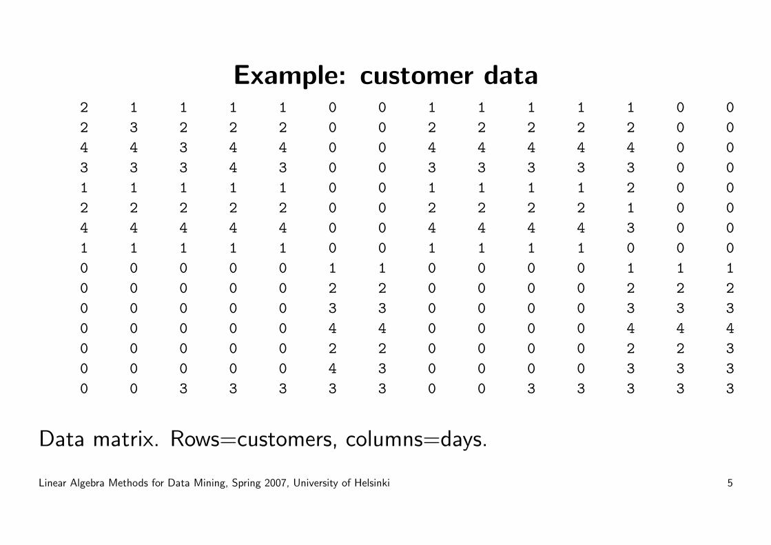
Example: customer data2 1 1 1 1 0 0 1 1 1 1 1 0 02 3 2 2 2 0 0 2 2 2 2 2 0 04 4 3 4 4 0 0 4 4 4 4 4 0 03 3 3 4 3 0 0 3 3 3 3 3 0 01 1 1 1 1 0 0 1 1 1 1 2 0 02 2 2 2 2 0 0 2 2 2 2 1 0 04 4 4 4 4 0 0 4 4 4 4 3 0 01 1 1 1 1 0 0 1 1 1 1 0 0 00 0 0 0 0 1 1 0 0 0 0 1 1 10 0 0 0 0 2 2 0 0 0 0 2 2 20 0 0 0 0 3 3 0 0 0 0 3 3 30 0 0 0 0 4 4 0 0 0 0 4 4 40 0 0 0 0 2 2 0 0 0 0 2 2 30 0 0 0 0 4 3 0 0 0 0 3 3 30 0 3 3 3 3 3 0 0 3 3 3 3 3
Data matrix. Rows=customers, columns=days.
Linear Algebra Methods for Data Mining, Spring 2007, University of Helsinki 5
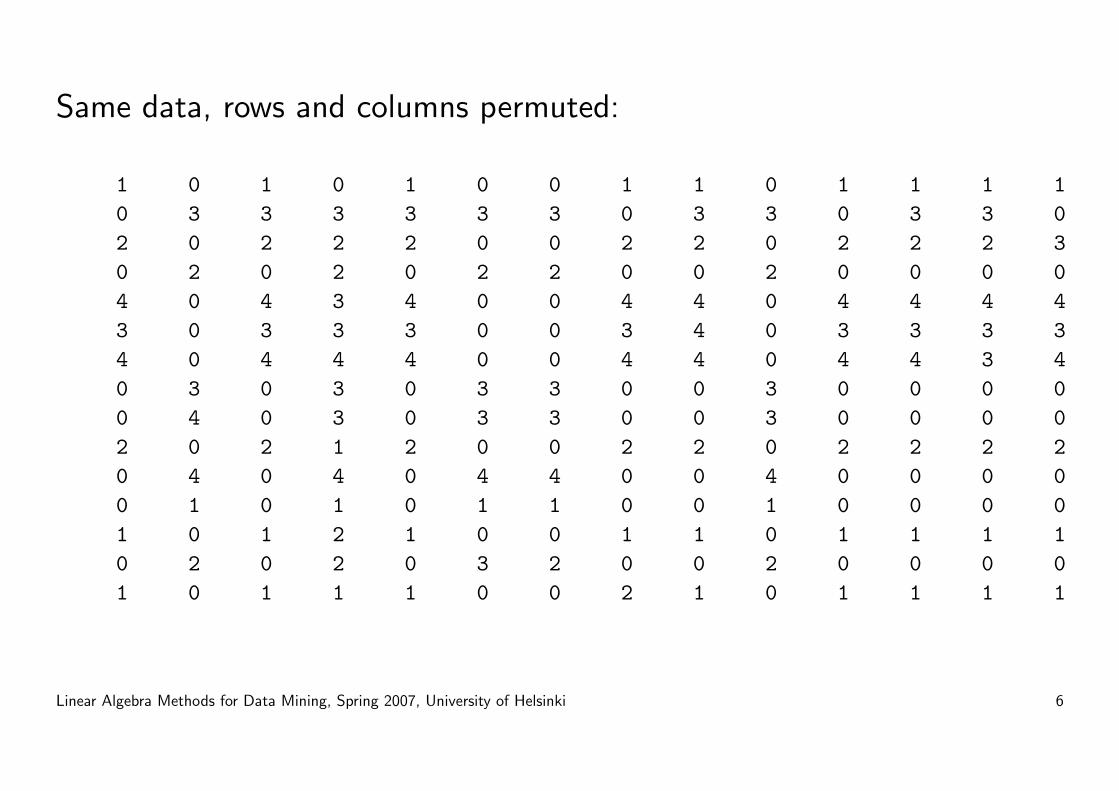
Same data, rows and columns permuted:
1 0 1 0 1 0 0 1 1 0 1 1 1 10 3 3 3 3 3 3 0 3 3 0 3 3 02 0 2 2 2 0 0 2 2 0 2 2 2 30 2 0 2 0 2 2 0 0 2 0 0 0 04 0 4 3 4 0 0 4 4 0 4 4 4 43 0 3 3 3 0 0 3 4 0 3 3 3 34 0 4 4 4 0 0 4 4 0 4 4 3 40 3 0 3 0 3 3 0 0 3 0 0 0 00 4 0 3 0 3 3 0 0 3 0 0 0 02 0 2 1 2 0 0 2 2 0 2 2 2 20 4 0 4 0 4 4 0 0 4 0 0 0 00 1 0 1 0 1 1 0 0 1 0 0 0 01 0 1 2 1 0 0 1 1 0 1 1 1 10 2 0 2 0 3 2 0 0 2 0 0 0 01 0 1 1 1 0 0 2 1 0 1 1 1 1
Linear Algebra Methods for Data Mining, Spring 2007, University of Helsinki 6
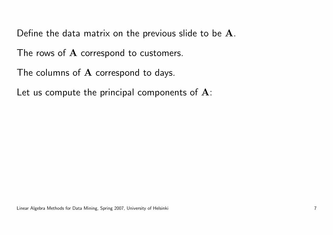
Define the data matrix on the previous slide to be A.
The rows of A correspond to customers.
The columns of A correspond to days.
Let us compute the principal components of A:
Linear Algebra Methods for Data Mining, Spring 2007, University of Helsinki 7
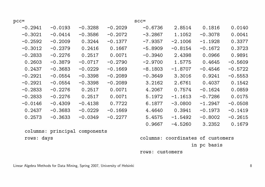
pcc=-0.2941 -0.0193 -0.3288 -0.2029-0.3021 -0.0414 -0.3586 -0.2072-0.2592 -0.2009 0.3244 -0.1377-0.3012 -0.2379 0.2416 0.1667-0.2833 -0.2276 0.2517 0.00710.2603 -0.3879 -0.0717 -0.27900.2437 -0.3683 -0.0229 -0.1669
-0.2921 -0.0554 -0.3398 -0.2089-0.2921 -0.0554 -0.3398 -0.2089-0.2833 -0.2276 0.2517 0.0071-0.2833 -0.2276 0.2517 0.0071-0.0146 -0.4309 -0.4138 0.77220.2437 -0.3683 -0.0229 -0.16690.2573 -0.3633 -0.0349 -0.2277
columns: principal componentsrows: days
scc=-0.6736 2.8514 0.1816 0.0140-3.2867 1.1052 -0.3078 0.0041-7.9357 -2.1006 -1.1928 0.3377-5.8909 -0.8154 -0.1672 0.3723-0.3940 2.4398 0.0966 0.9891-2.9700 1.5775 0.4645 -0.5609-8.1803 -1.8707 -0.4546 -0.5722-0.3649 3.3016 0.9241 -0.55533.2162 2.6761 0.4037 0.15424.2067 0.7574 -0.1624 0.08595.1972 -1.1613 -0.7286 0.01756.1877 -3.0800 -1.2947 -0.05084.4640 0.3941 -0.1973 -0.14195.4575 -1.5492 -0.8002 -0.26150.9667 -4.5260 3.2352 0.1679
columns: coordinates of customersin pc basis
rows: customers
Linear Algebra Methods for Data Mining, Spring 2007, University of Helsinki 8
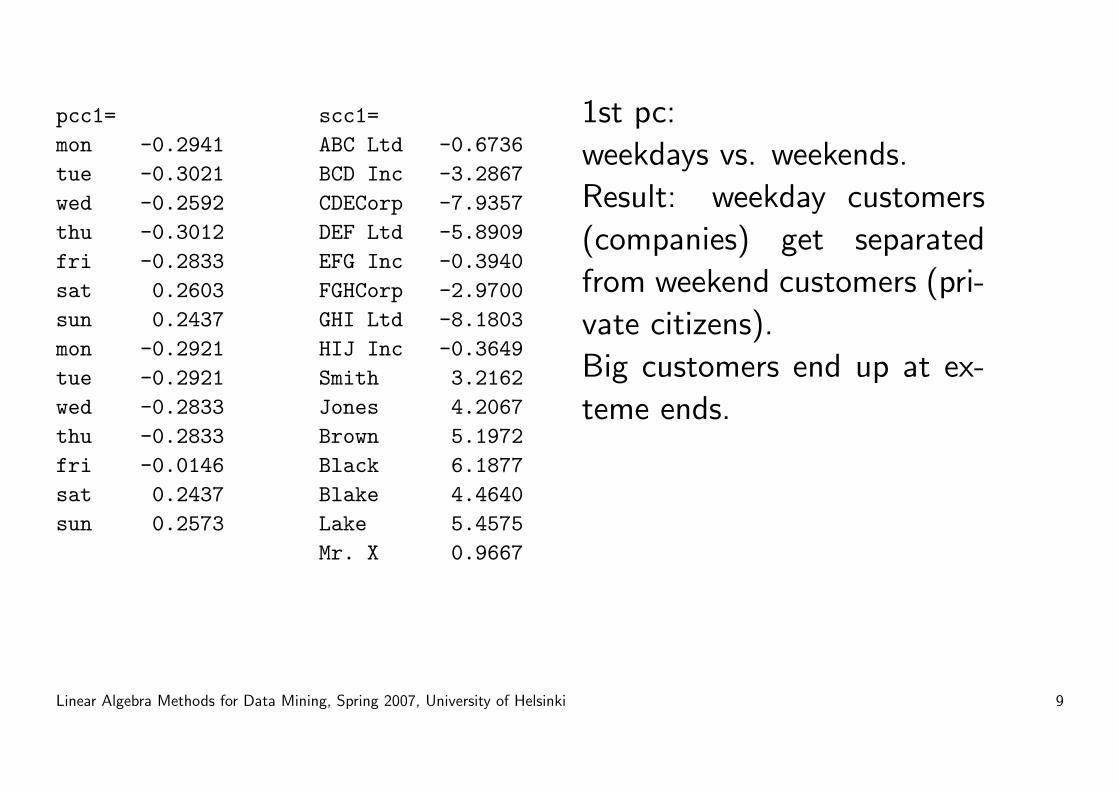
pcc1=mon -0.2941tue -0.3021wed -0.2592thu -0.3012fri -0.2833sat 0.2603sun 0.2437mon -0.2921tue -0.2921wed -0.2833thu -0.2833fri -0.0146sat 0.2437sun 0.2573
scc1=ABC Ltd -0.6736BCD Inc -3.2867CDECorp -7.9357DEF Ltd -5.8909EFG Inc -0.3940FGHCorp -2.9700GHI Ltd -8.1803HIJ Inc -0.3649Smith 3.2162Jones 4.2067Brown 5.1972Black 6.1877Blake 4.4640Lake 5.4575Mr. X 0.9667
1st pc:
weekdays vs. weekends.
Result: weekday customers
(companies) get separated
from weekend customers (pri-
vate citizens).
Big customers end up at ex-
teme ends.
Linear Algebra Methods for Data Mining, Spring 2007, University of Helsinki 9
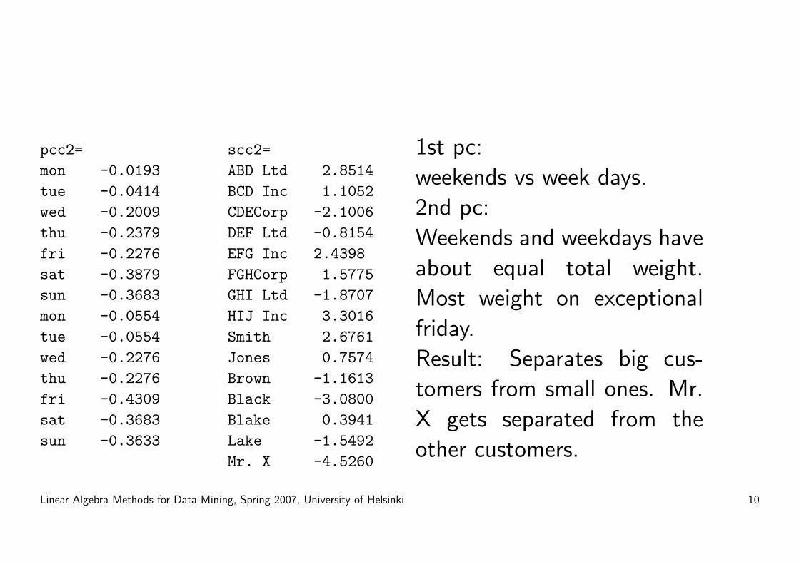
pcc2=mon -0.0193tue -0.0414wed -0.2009thu -0.2379fri -0.2276sat -0.3879sun -0.3683mon -0.0554tue -0.0554wed -0.2276thu -0.2276fri -0.4309sat -0.3683sun -0.3633
scc2=ABD Ltd 2.8514BCD Inc 1.1052CDECorp -2.1006DEF Ltd -0.8154EFG Inc 2.4398FGHCorp 1.5775GHI Ltd -1.8707HIJ Inc 3.3016Smith 2.6761Jones 0.7574Brown -1.1613Black -3.0800Blake 0.3941Lake -1.5492Mr. X -4.5260
1st pc:
weekends vs week days.
2nd pc:
Weekends and weekdays have
about equal total weight.
Most weight on exceptional
friday.
Result: Separates big cus-
tomers from small ones. Mr.
X gets separated from the
other customers.
Linear Algebra Methods for Data Mining, Spring 2007, University of Helsinki 10
−10 −8 −6 −4 −2 0 2 4 6 8−5
−4
−3
−2
−1
0
1
2
3
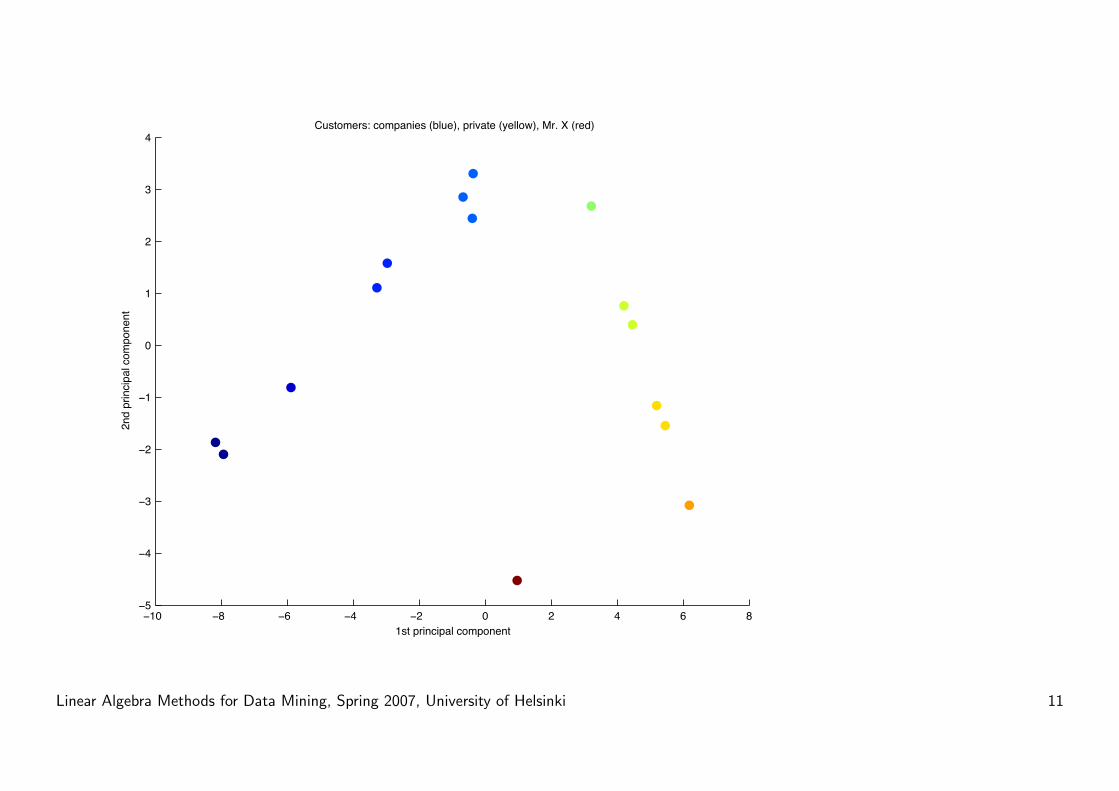
4Customers: companies (blue), private (yellow), Mr. X (red)
1st principal component
2nd
prin
cipa
l com
pone
nt
Linear Algebra Methods for Data Mining, Spring 2007, University of Helsinki 11
−10 −8 −6 −4 −2 0 2 4 6 8−3.5
−3
−2.5
−2
−1.5
−1
−0.5
0
0.5
1
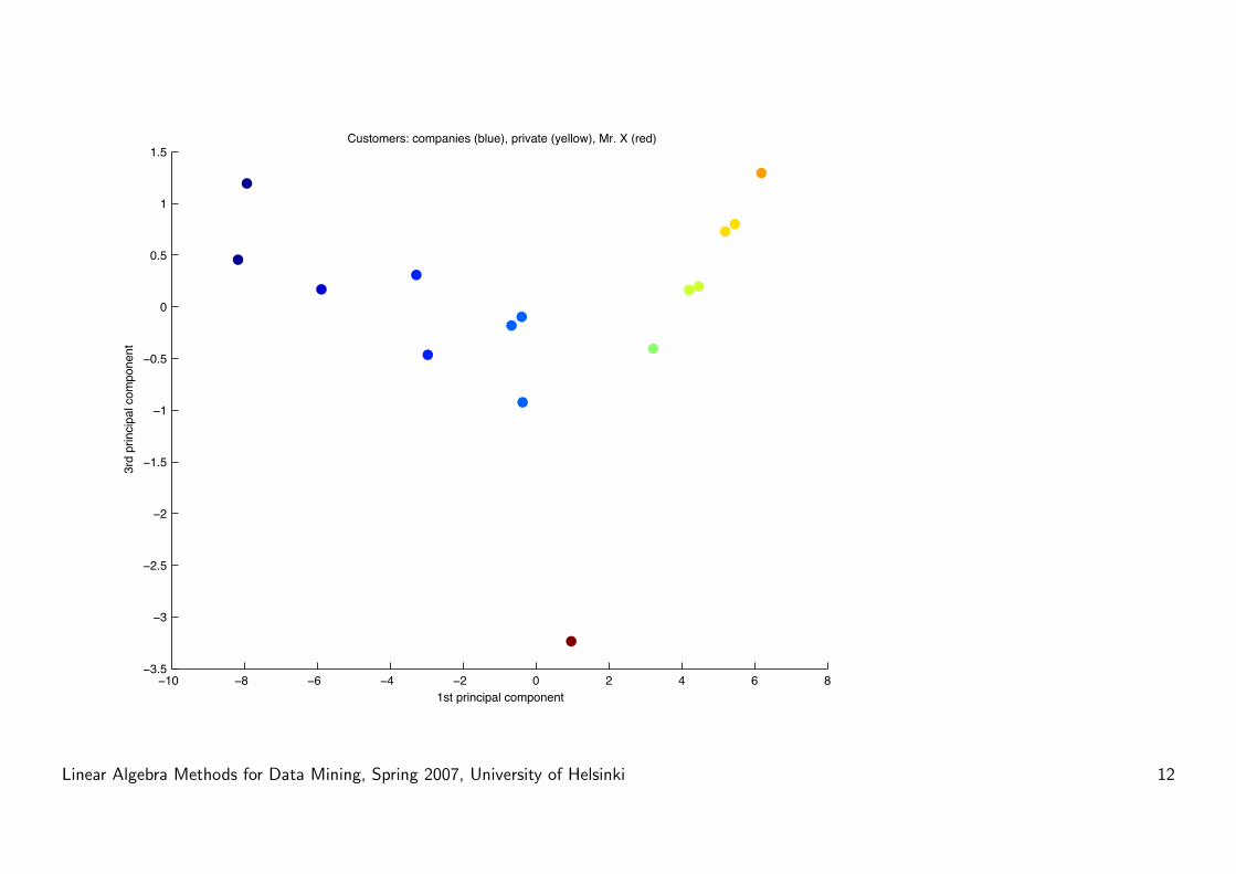
1.5Customers: companies (blue), private (yellow), Mr. X (red)
1st principal component
3rd
prin
cipa
l com
pone
nt
Linear Algebra Methods for Data Mining, Spring 2007, University of Helsinki 12
What if we transpose our problem?
Instead of thinking of customers as our data points, why not think of days
as our data points, and customers as the attributes/variables?
The rows of A correspond to days.
The columns of A correspond to customers.
Let us compute the principal components of A:
Linear Algebra Methods for Data Mining, Spring 2007, University of Helsinki 13
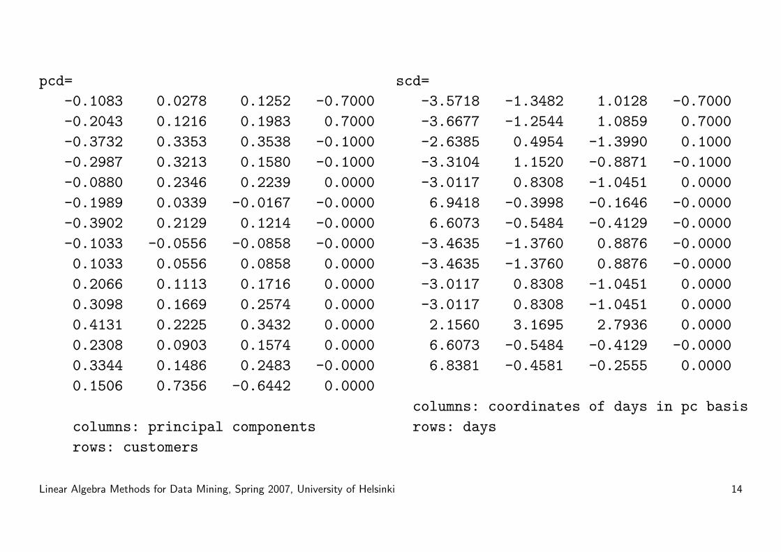
pcd=-0.1083 0.0278 0.1252 -0.7000-0.2043 0.1216 0.1983 0.7000-0.3732 0.3353 0.3538 -0.1000-0.2987 0.3213 0.1580 -0.1000-0.0880 0.2346 0.2239 0.0000-0.1989 0.0339 -0.0167 -0.0000-0.3902 0.2129 0.1214 -0.0000-0.1033 -0.0556 -0.0858 -0.00000.1033 0.0556 0.0858 0.00000.2066 0.1113 0.1716 0.00000.3098 0.1669 0.2574 0.00000.4131 0.2225 0.3432 0.00000.2308 0.0903 0.1574 0.00000.3344 0.1486 0.2483 -0.00000.1506 0.7356 -0.6442 0.0000
columns: principal componentsrows: customers
scd=-3.5718 -1.3482 1.0128 -0.7000-3.6677 -1.2544 1.0859 0.7000-2.6385 0.4954 -1.3990 0.1000-3.3104 1.1520 -0.8871 -0.1000-3.0117 0.8308 -1.0451 0.00006.9418 -0.3998 -0.1646 -0.00006.6073 -0.5484 -0.4129 -0.0000
-3.4635 -1.3760 0.8876 -0.0000-3.4635 -1.3760 0.8876 -0.0000-3.0117 0.8308 -1.0451 0.0000-3.0117 0.8308 -1.0451 0.00002.1560 3.1695 2.7936 0.00006.6073 -0.5484 -0.4129 -0.00006.8381 -0.4581 -0.2555 0.0000
columns: coordinates of days in pc basisrows: days
Linear Algebra Methods for Data Mining, Spring 2007, University of Helsinki 14
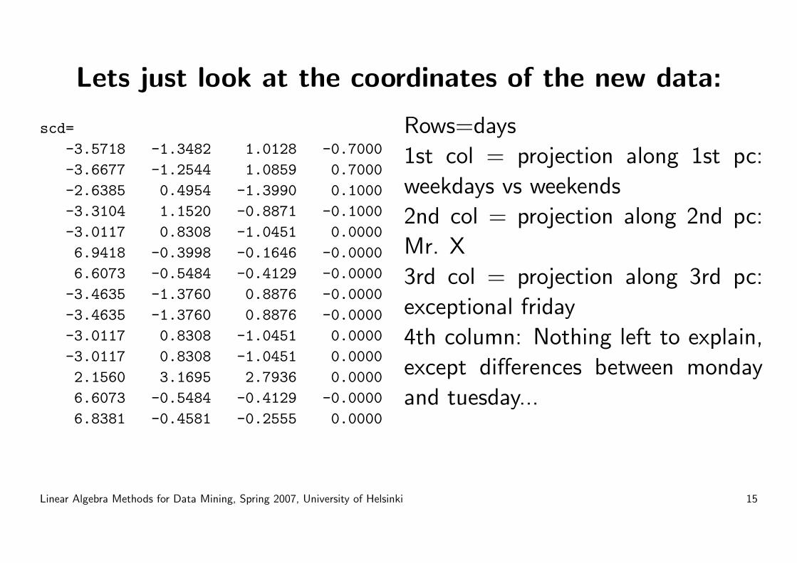
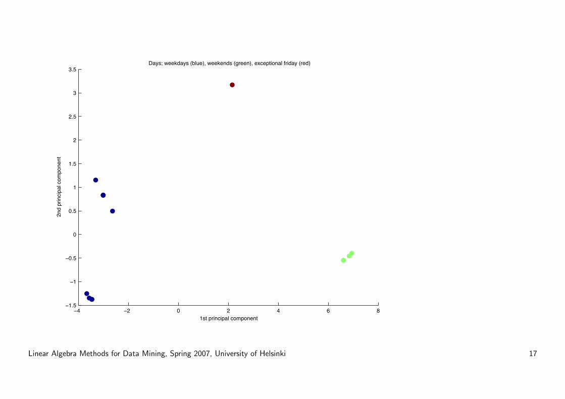
Lets just look at the coordinates of the new data:
scd=-3.5718 -1.3482 1.0128 -0.7000-3.6677 -1.2544 1.0859 0.7000-2.6385 0.4954 -1.3990 0.1000-3.3104 1.1520 -0.8871 -0.1000-3.0117 0.8308 -1.0451 0.00006.9418 -0.3998 -0.1646 -0.00006.6073 -0.5484 -0.4129 -0.0000
-3.4635 -1.3760 0.8876 -0.0000-3.4635 -1.3760 0.8876 -0.0000-3.0117 0.8308 -1.0451 0.0000-3.0117 0.8308 -1.0451 0.00002.1560 3.1695 2.7936 0.00006.6073 -0.5484 -0.4129 -0.00006.8381 -0.4581 -0.2555 0.0000
Rows=days
1st col = projection along 1st pc:
weekdays vs weekends
2nd col = projection along 2nd pc:
Mr. X
3rd col = projection along 3rd pc:
exceptional friday
4th column: Nothing left to explain,
except differences between monday
and tuesday...
Linear Algebra Methods for Data Mining, Spring 2007, University of Helsinki 15
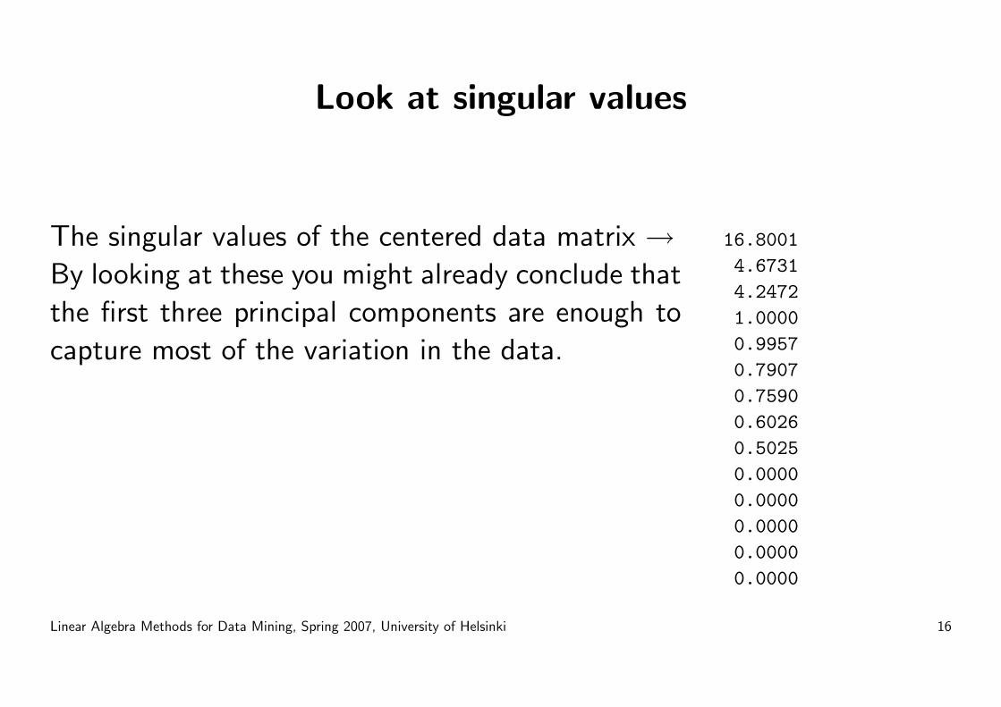
Look at singular values
The singular values of the centered data matrix →By looking at these you might already conclude that
the first three principal components are enough to
capture most of the variation in the data.
16.80014.67314.24721.00000.99570.79070.75900.60260.50250.00000.00000.00000.00000.0000
Linear Algebra Methods for Data Mining, Spring 2007, University of Helsinki 16
−4 −2 0 2 4 6 8−1.5
−1
−0.5
0
0.5
1
1.5
2
2.5
3
3.5Days; weekdays (blue), weekends (green), exceptional friday (red)
1st principal component
2nd
prin
cipa
l com
pone
nt
Linear Algebra Methods for Data Mining, Spring 2007, University of Helsinki 17
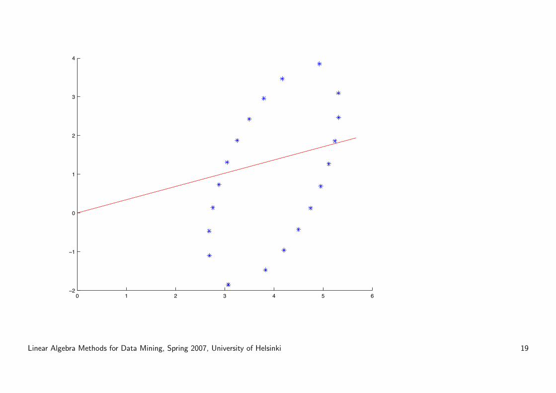
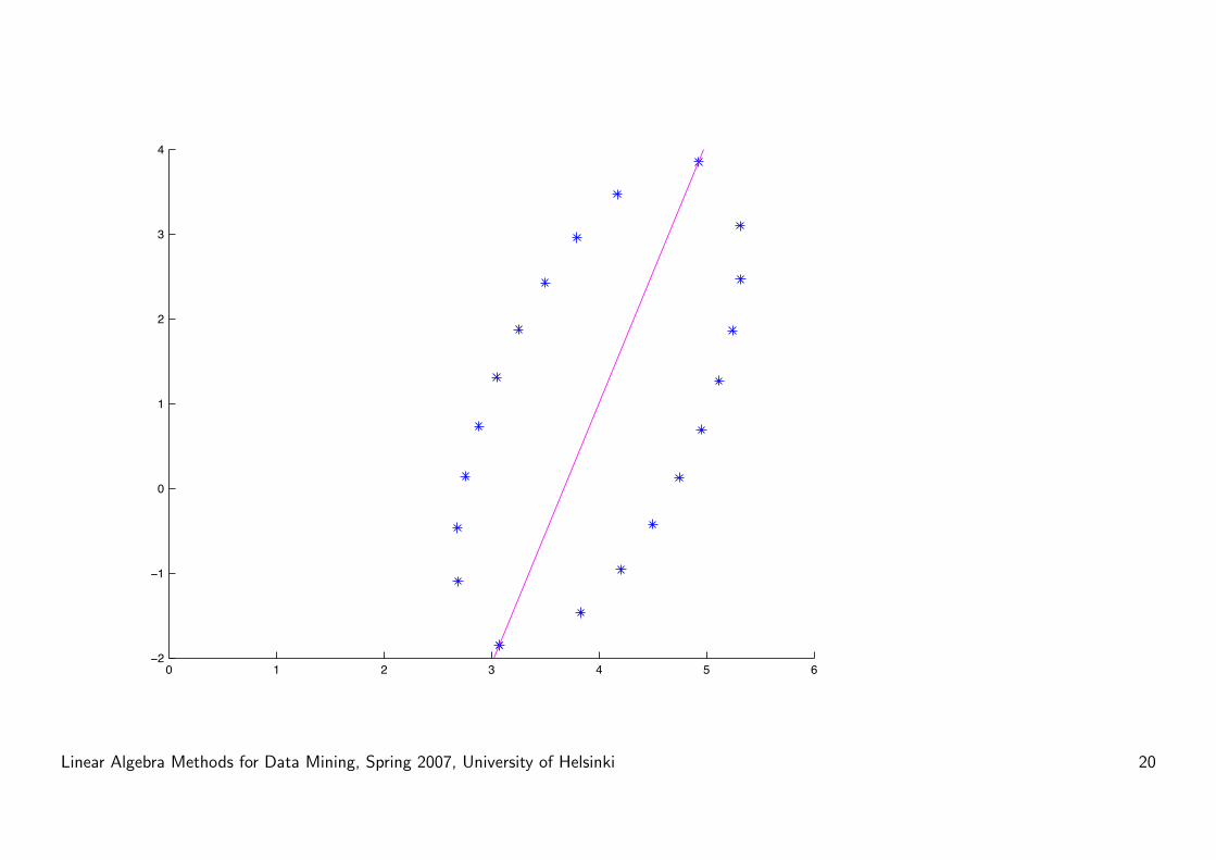
SVD vs PCA: Centering is central
SVD will give vectors that go through the origin.
Centering makes sure that the origin is in the middle of the data set.
Linear Algebra Methods for Data Mining, Spring 2007, University of Helsinki 18
0 1 2 3 4 5 6−2
−1
0
1
2
3
4
Linear Algebra Methods for Data Mining, Spring 2007, University of Helsinki 19
0 1 2 3 4 5 6−2
−1
0
1
2
3
4
Linear Algebra Methods for Data Mining, Spring 2007, University of Helsinki 20
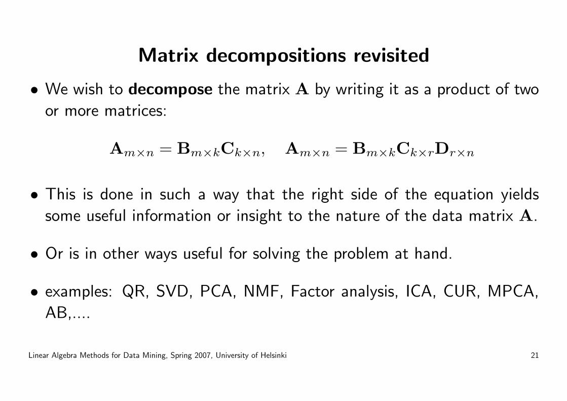
Matrix decompositions revisited
• We wish to decompose the matrix A by writing it as a product of two
or more matrices:
Am×n = Bm×kCk×n, Am×n = Bm×kCk×rDr×n
• This is done in such a way that the right side of the equation yields
some useful information or insight to the nature of the data matrix A.
• Or is in other ways useful for solving the problem at hand.
• examples: QR, SVD, PCA, NMF, Factor analysis, ICA, CUR, MPCA,
AB,....
Linear Algebra Methods for Data Mining, Spring 2007, University of Helsinki 21
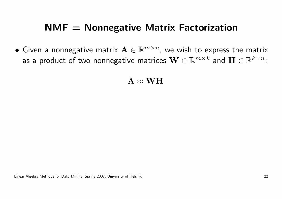
NMF = Nonnegative Matrix Factorization
• Given a nonnegative matrix A ∈ Rm×n, we wish to express the matrix
as a product of two nonnegative matrices W ∈ Rm×k and H ∈ Rk×n:
A ≈ WH
Linear Algebra Methods for Data Mining, Spring 2007, University of Helsinki 22
Why require nonnegativity?
• nonnegativity is natural in many applications...
• term-document
• market basket
• etc
Linear Algebra Methods for Data Mining, Spring 2007, University of Helsinki 23
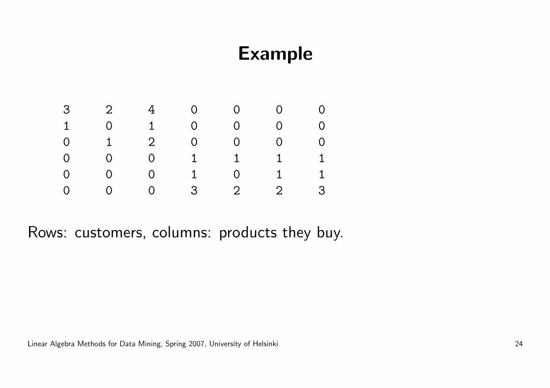
Example
3 2 4 0 0 0 01 0 1 0 0 0 00 1 2 0 0 0 00 0 0 1 1 1 10 0 0 1 0 1 10 0 0 3 2 2 3
Rows: customers, columns: products they buy.
Linear Algebra Methods for Data Mining, Spring 2007, University of Helsinki 24
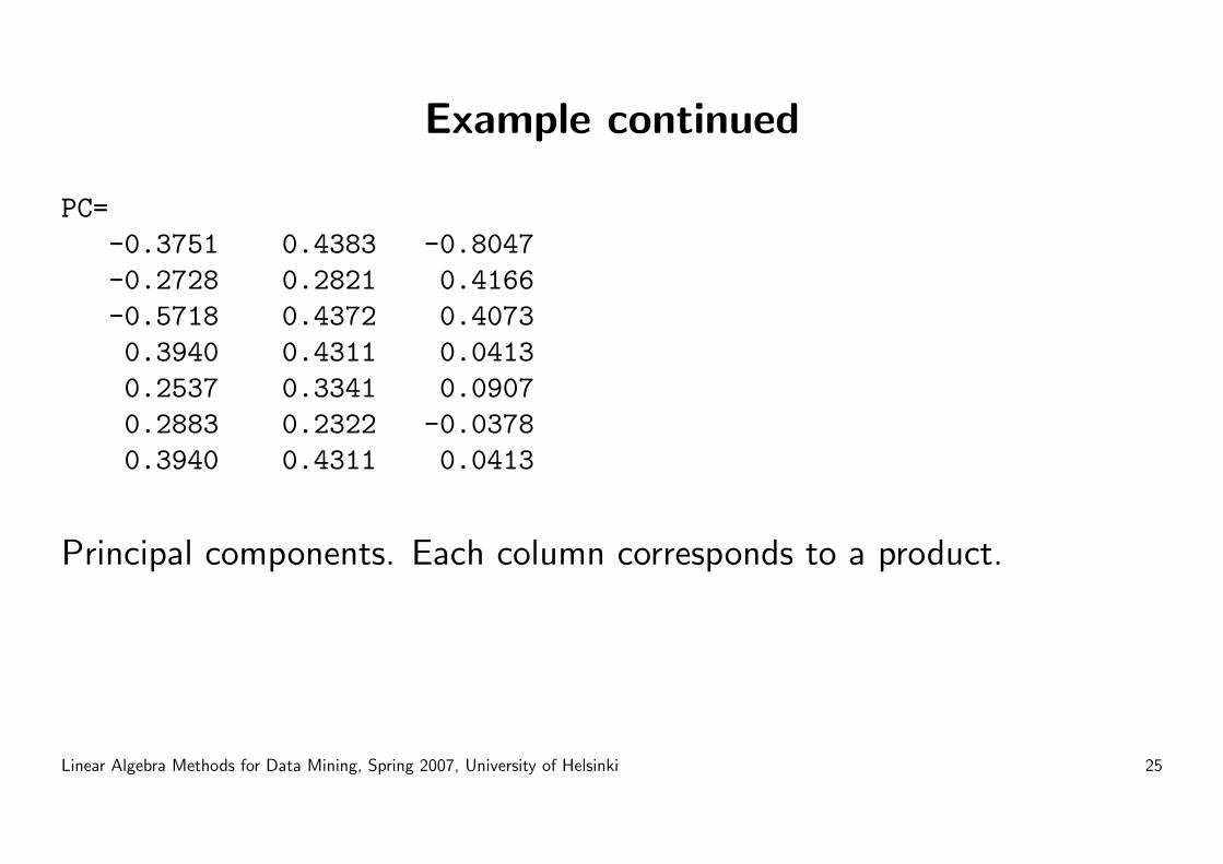
Example continued
PC=-0.3751 0.4383 -0.8047-0.2728 0.2821 0.4166-0.5718 0.4372 0.40730.3940 0.4311 0.04130.2537 0.3341 0.09070.2883 0.2322 -0.03780.3940 0.4311 0.0413
Principal components. Each column corresponds to a product.
Linear Algebra Methods for Data Mining, Spring 2007, University of Helsinki 25
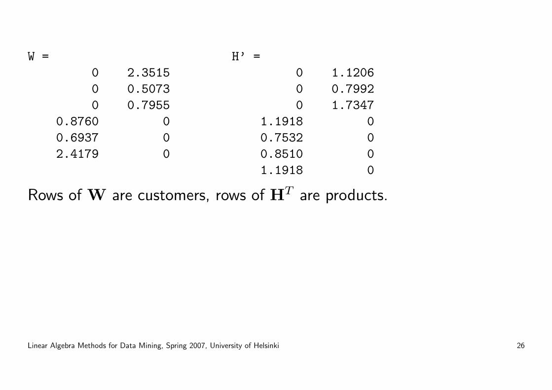
W =0 2.35150 0.50730 0.7955
0.8760 00.6937 02.4179 0
H’ =0 1.12060 0.79920 1.7347
1.1918 00.7532 00.8510 01.1918 0
Rows of W are customers, rows of HT are products.
Linear Algebra Methods for Data Mining, Spring 2007, University of Helsinki 26
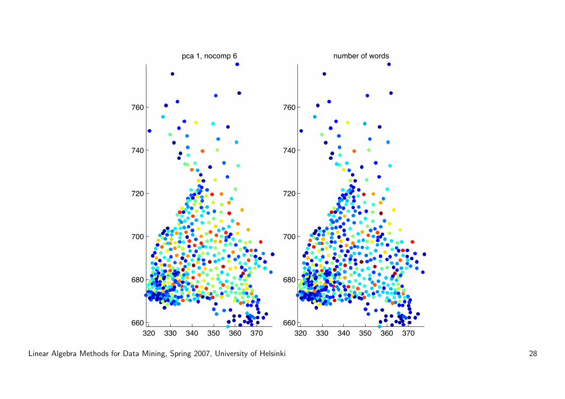
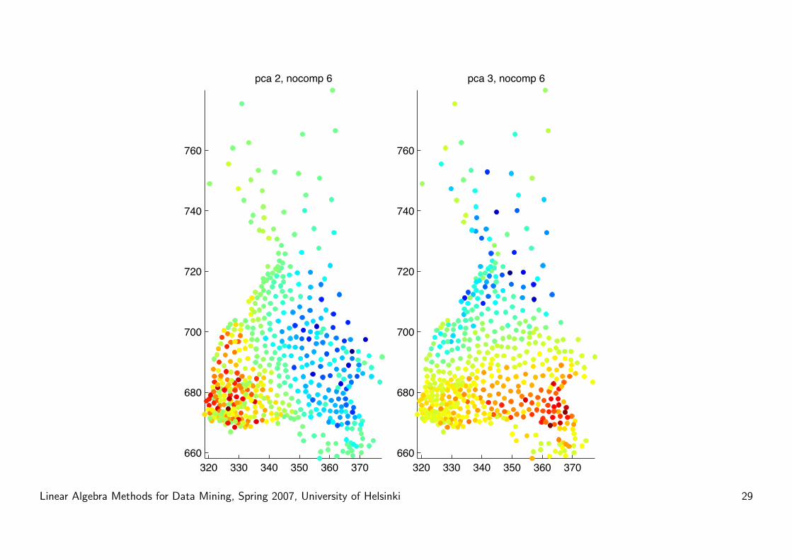
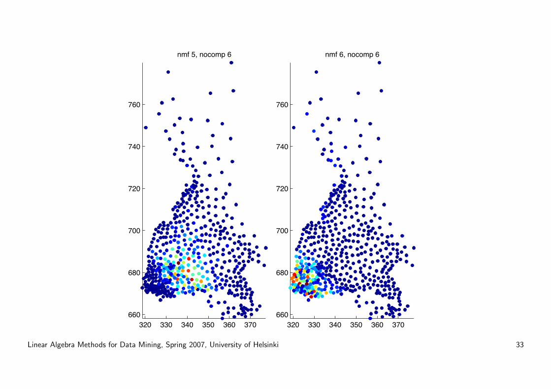
Example: finnish dialects revisited
• Data: 17000 dialect words, 500 counties.
• Word-county matrix A:
A(i, j) ={
1 if word i appears in county j
0 otherwise.
• Apply PCA to this: data points: words, variables: counties
• Each principal component tells which counties explain the most signifi-
cant part of the variation left in the data.
Linear Algebra Methods for Data Mining, Spring 2007, University of Helsinki 27
320 330 340 350 360 370660
680
700
720
740
760
pca 1, nocomp 6
320 330 340 350 360 370660
680
700
720
740
760
number of words
Linear Algebra Methods for Data Mining, Spring 2007, University of Helsinki 28
320 330 340 350 360 370660
680
700
720
740
760
pca 2, nocomp 6
320 330 340 350 360 370660
680
700
720
740
760
pca 3, nocomp 6
Linear Algebra Methods for Data Mining, Spring 2007, University of Helsinki 29
• Gives a general idea of how dialects vary...
• But (in general) does not capture local structure very well!
• What we would like would be a decomposition, where the components
represent contributions of single dialects.
• NMF?
Linear Algebra Methods for Data Mining, Spring 2007, University of Helsinki 30
320 330 340 350 360 370660
680
700
720
740
760
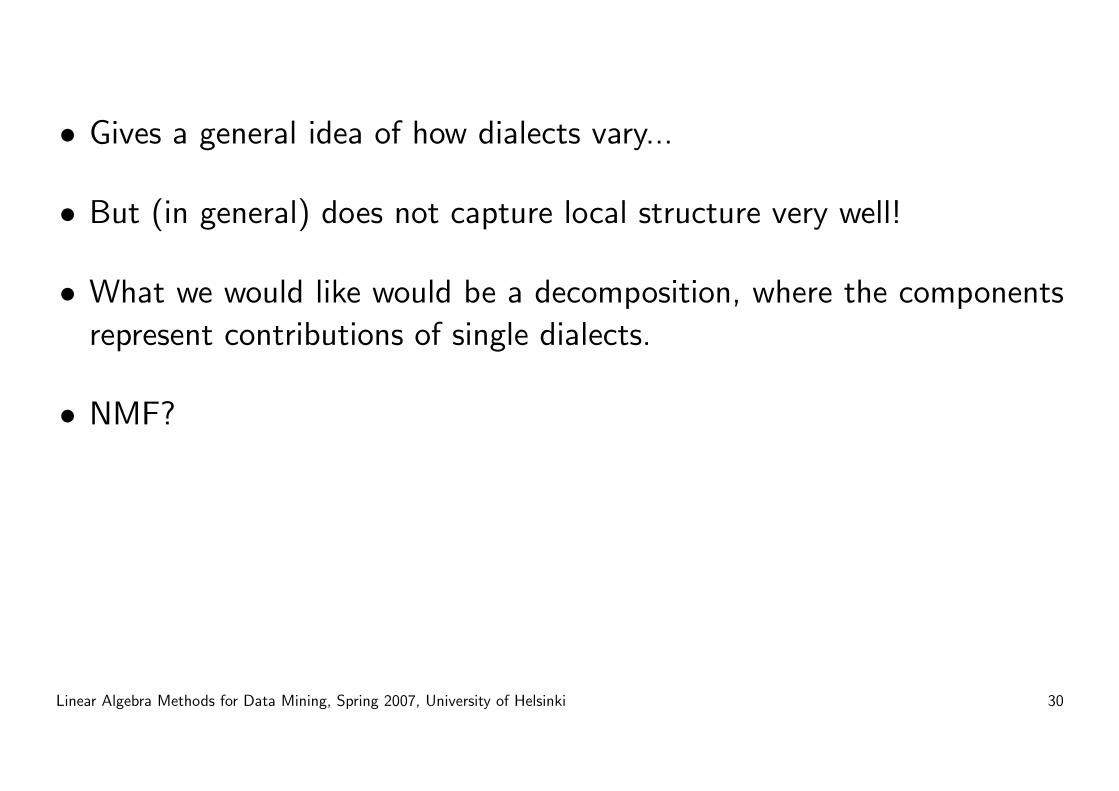
nmf 1, nocomp 6
320 330 340 350 360 370660
680
700
720
740
760
nmf 2, nocomp 6
Linear Algebra Methods for Data Mining, Spring 2007, University of Helsinki 31
320 330 340 350 360 370660
680
700
720
740
760
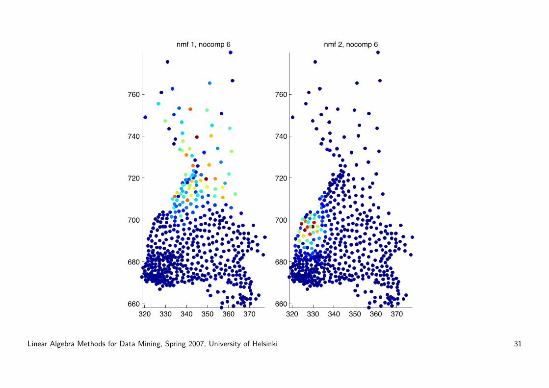
nmf 3, nocomp 6
320 330 340 350 360 370660
680
700
720
740
760
nmf 4, nocomp 6
Linear Algebra Methods for Data Mining, Spring 2007, University of Helsinki 32
320 330 340 350 360 370660
680
700
720
740
760
nmf 5, nocomp 6
320 330 340 350 360 370660
680
700
720
740
760
nmf 6, nocomp 6
Linear Algebra Methods for Data Mining, Spring 2007, University of Helsinki 33
Results
• More local structure
• Components correspond to dialect regions
• Interpretation:
A = WH
where W ∈ Rm×k is the ”word per dialect region” matrix, and H ∈Rk×n is the ”dialect region per county” matrix.
Linear Algebra Methods for Data Mining, Spring 2007, University of Helsinki 34
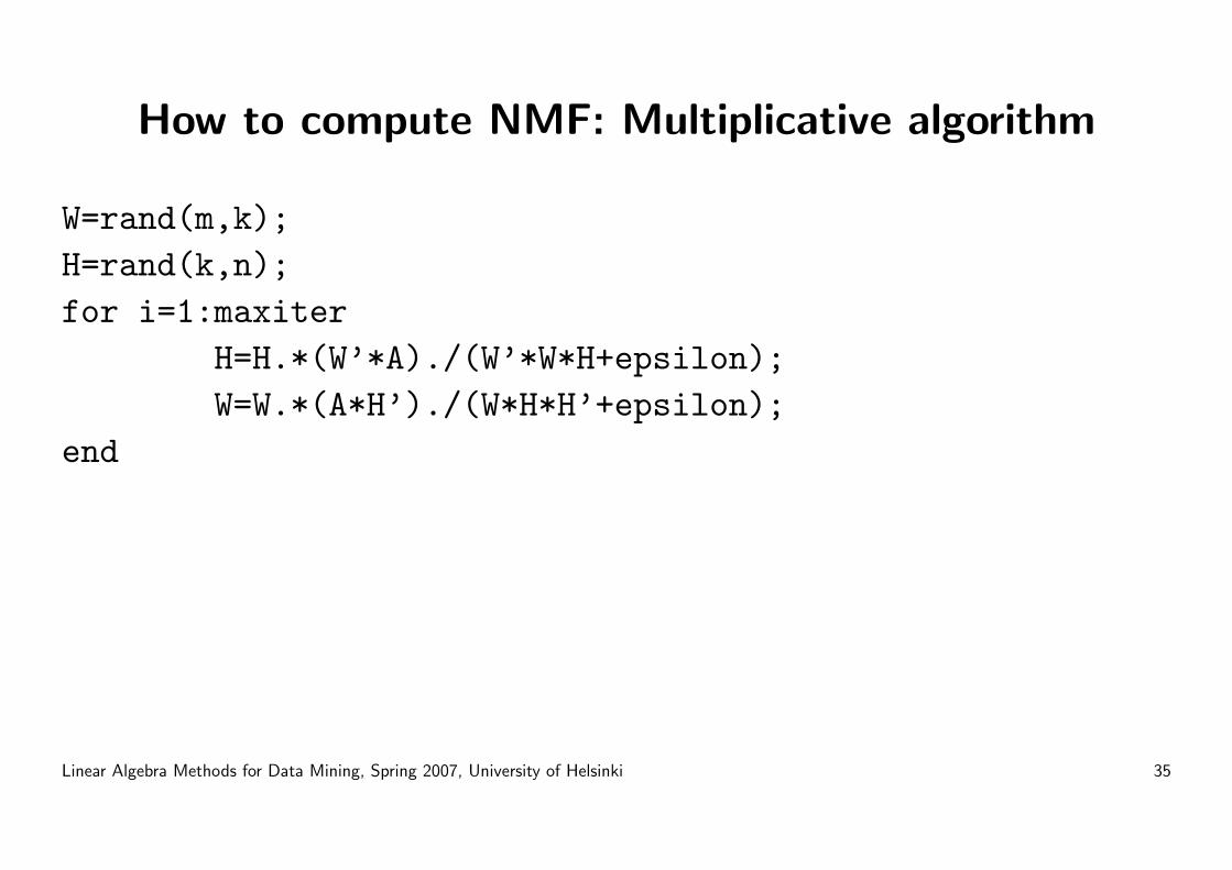
How to compute NMF: Multiplicative algorithm
W=rand(m,k);H=rand(k,n);for i=1:maxiter
H=H.*(W’*A)./(W’*W*H+epsilon);W=W.*(A*H’)./(W*H*H’+epsilon);
end
Linear Algebra Methods for Data Mining, Spring 2007, University of Helsinki 35
Comments on the multiplicative algorithm
• Easy to implement.
• Convergence?
• Once an element is zero, it stays zero.
Linear Algebra Methods for Data Mining, Spring 2007, University of Helsinki 36
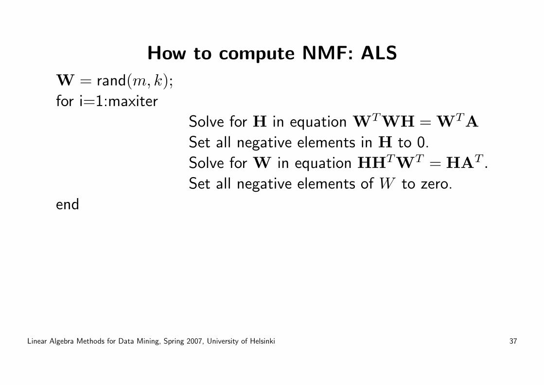
How to compute NMF: ALS
W = rand(m, k);for i=1:maxiter
Solve for H in equation WTWH = WTASet all negative elements in H to 0.
Solve for W in equation HHTWT = HAT .
Set all negative elements of W to zero.
end
Linear Algebra Methods for Data Mining, Spring 2007, University of Helsinki 37
Comments on the ALS algorithm
• Can be very fast (depending on implementation)
• Convergence?
• Sparsity
• Improved versions exist
Linear Algebra Methods for Data Mining, Spring 2007, University of Helsinki 38
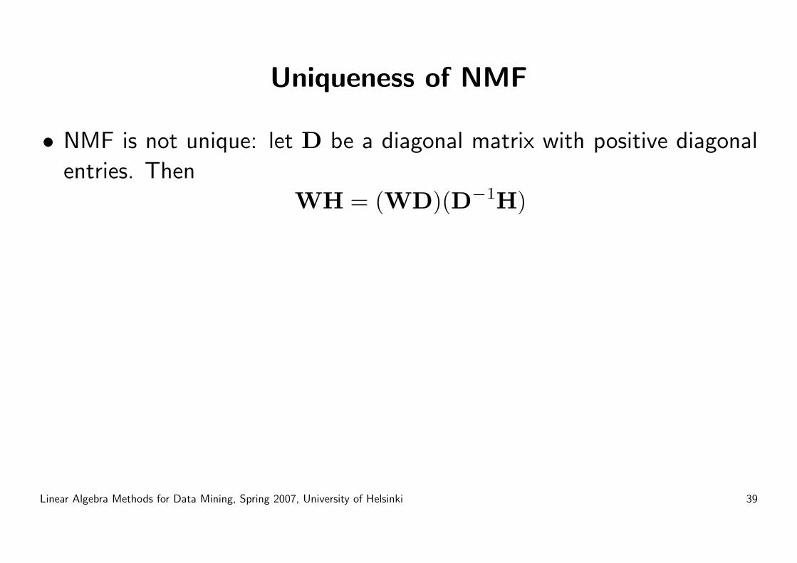
Uniqueness of NMF
• NMF is not unique: let D be a diagonal matrix with positive diagonal
entries. Then
WH = (WD)(D−1H)
Linear Algebra Methods for Data Mining, Spring 2007, University of Helsinki 39
Initialization
• Convergence can be slow.
• It can be speeded up using a good initial guess: initialization.
• A good initialization can be found using SVD (see p. 106)
Linear Algebra Methods for Data Mining, Spring 2007, University of Helsinki 40
Summary
• Given a nonnegative matrix A ∈ Rm×n find nonnegative matrices
W ∈ Rm×k and H ∈ Rk×n so that
‖A−WH‖
is minimized.
• Algorithms exist, both basic (easy to implement) and more advanced
(implementing e.g. sparsity constraints)
• Interpretability
Linear Algebra Methods for Data Mining, Spring 2007, University of Helsinki 41
Applications
• text mining
• email surveillance
• music transcription
• bioinformatics
• source separation
• spatial data analysis
• etc
Linear Algebra Methods for Data Mining, Spring 2007, University of Helsinki 42
References
[1] Lars Elden: Matrix Methods in Data Mining and Pattern Recognition,
SIAM 2007.
[2] Berry, Browne, Langville, Pauca, Plemmons: Algorithms and Applica-
tions for Approximate Nonnegative Matrix Factorization
Linear Algebra Methods for Data Mining, Spring 2007, University of Helsinki 43
Recommended