
Leveraging Big Data: Lecture 12
Instructors:
http://www.cohenwang.com/edith/bigdataclass2013
Edith CohenAmos FiatHaim KaplanTova Milo
Today
All-Distances Sketches Applications of All-Distance sketches Back to linear sketches (random linear
transformations)
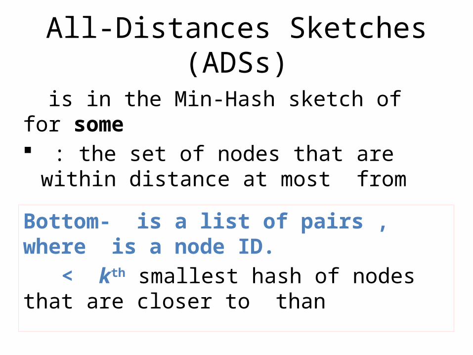
All-Distances Sketches (ADSs)
is in the Min-Hash sketch of for some : the set of nodes that are within distance at
most from
Bottom- is a list of pairs , where is a node ID. < kth smallest hash of nodes that are closer to than
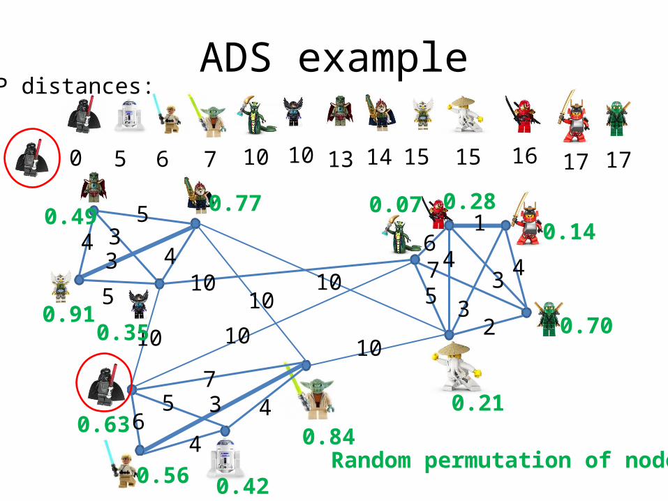
ADS example
5
5
4
433
101010
10 1010
65
7
675
3
4
1
2
43
3
44
13 14 15100 65 7 15 1716 1710
SP distances:
0.49
0.91
0.56 0.42
0.07
0.21
0.140.28
0.63 0.84
0.70
0.77
0.35
Random permutation of nodes
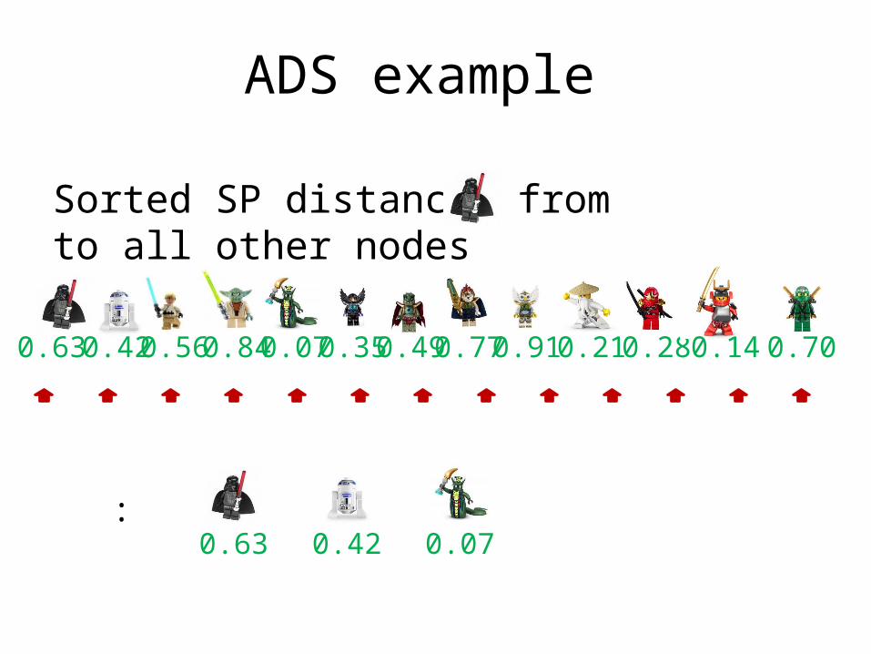
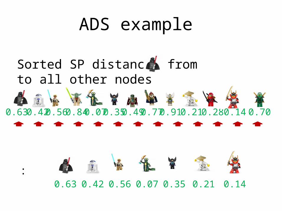
ADS example
Sorted SP distances from to all other nodes
0.63 0.42 0.56 0.84 0.07 0.35 0.49 0.91 0.21 0.28 0.14 0.700.77
:0.63 0.42 0.07
0.21
ADS example
:0.63 0.42 0.56 0.07 0.35 0.14
0.63 0.42 0.56 0.84 0.07 0.35 0.49 0.91 0.21 0.28 0.14 0.700.77
Sorted SP distances from to all other nodes
Expected Size of Bottom- ADS
Lemma: Proof: The ith closest node to is included with probability
* Same argument as in lecture2 to bound number of updates to a Min-Hash sketch of a stream. Distance instead of time.
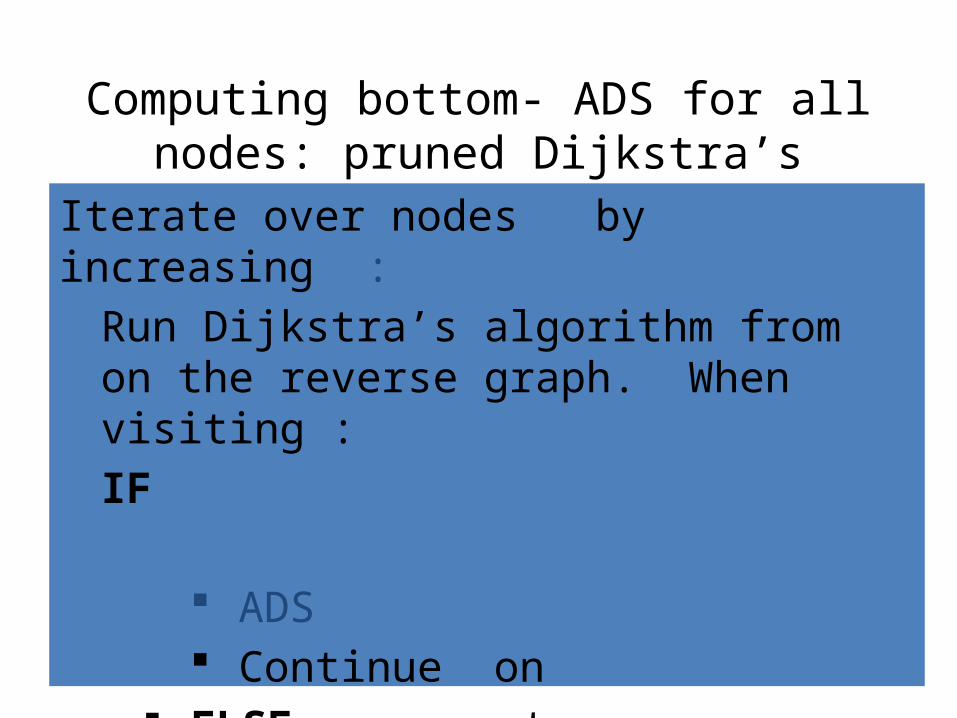
Computing bottom- ADS for all nodes: pruned Dijkstra’s
Iterate over nodes by increasing : Run Dijkstra’s algorithm from on the reverse graph. When visiting :IF
ADS Continue on
ELSE, prune at
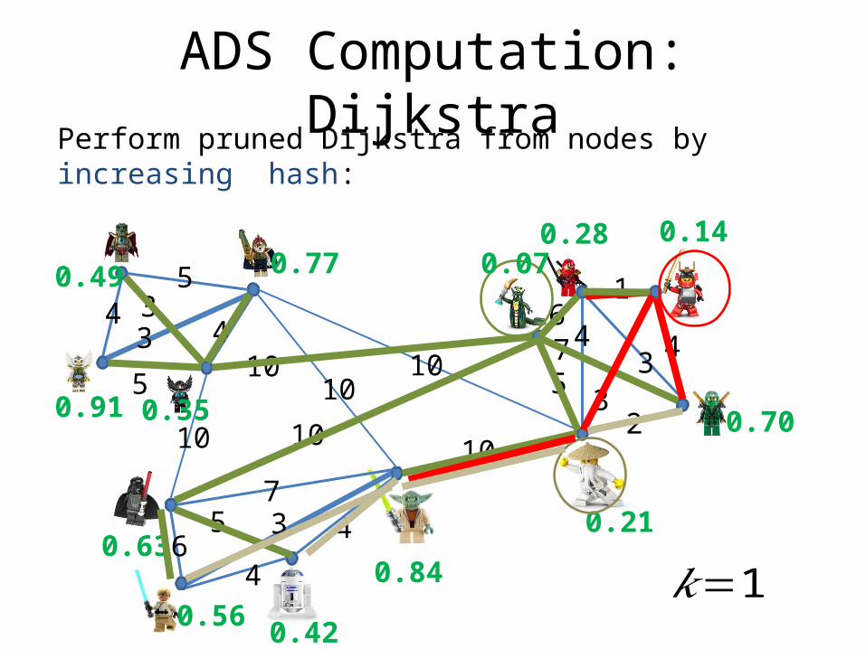
ADS Computation: DijkstraPerform pruned Dijkstra from nodes by increasing hash:
5
5
4
433
101010
10 1010
65
7
675
3
4
1
2
43
3
44
0.49
0.91
0.56 0.42
0.07
0.21
0.140.28
0.630.84
0.70
0.77
0.35
𝑘=1
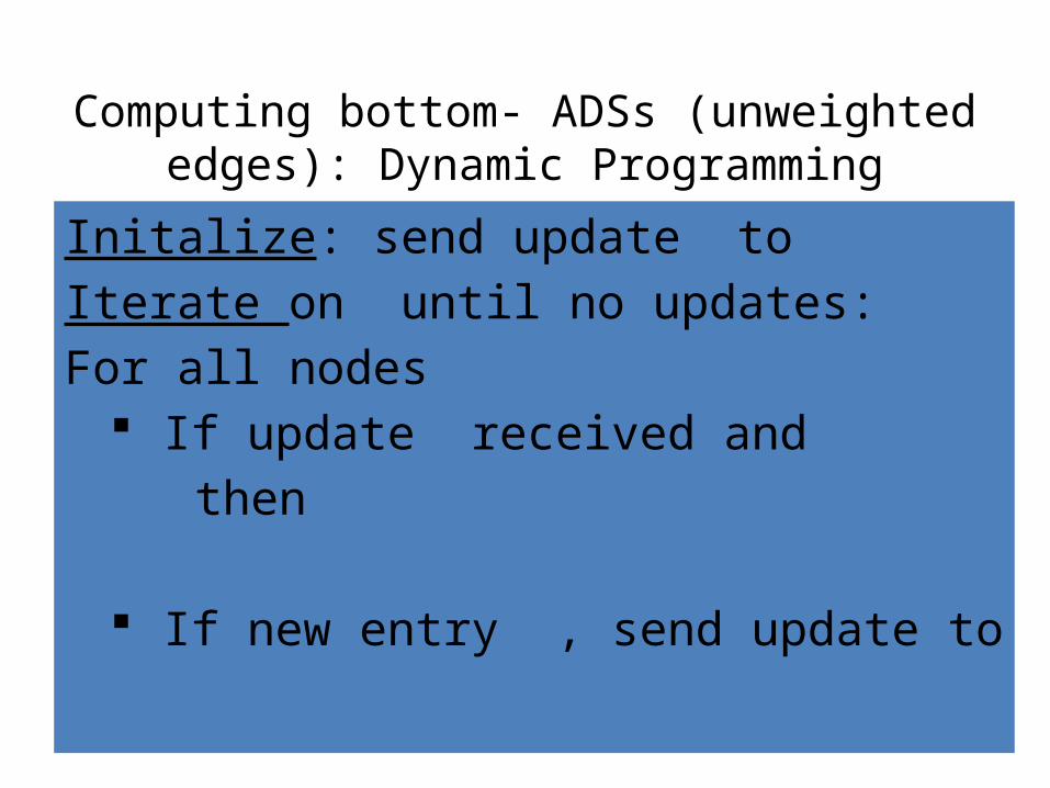
Computing bottom- ADSs (unweighted edges): Dynamic Programming
Initalize: send update to Iterate on until no updates:For all nodes
If update received and then If new entry , send update to
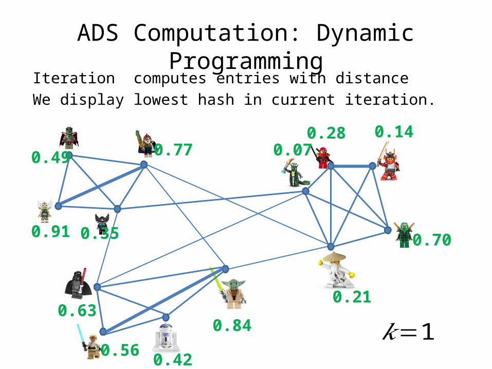
ADS Computation: Dynamic ProgrammingIteration computes entries with distance We display lowest hash in current iteration.
0.49
0.91
0.56 0.42
0.07
0.21
0.140.28
0.630.84
0.70
0.77
0.35
𝑘=1
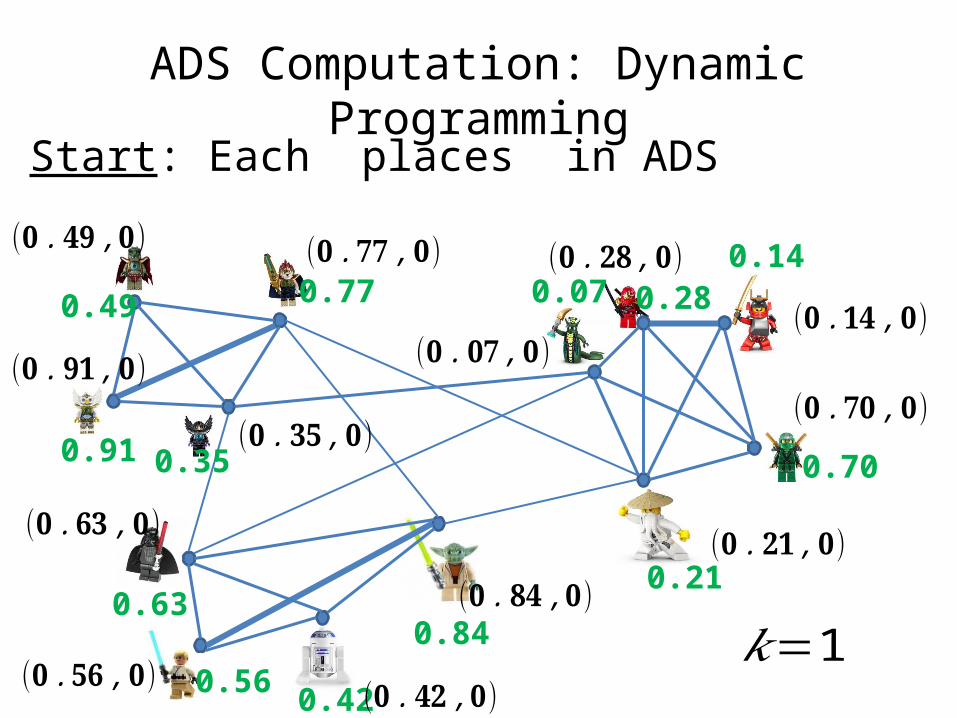
ADS Computation: Dynamic ProgrammingStart: Each places in ADS
0.49
0.91
0.56 0.42
0.07
0.21
0.140.28
0.630.84
0.70
0.77
0.35
𝑘=1
(𝟎 .𝟒𝟗 ,𝟎) (𝟎 .𝟕𝟕 ,𝟎)
(𝟎 .𝟎𝟕 ,𝟎)
(𝟎 .𝟐𝟖 ,𝟎)
(𝟎 .𝟏𝟒 ,𝟎)
(𝟎 .𝟕𝟎 ,𝟎)
(𝟎 .𝟐𝟏 ,𝟎)(𝟎 .𝟖𝟒 ,𝟎)
(𝟎 .𝟗𝟏 ,𝟎)
(𝟎 .𝟑𝟓 ,𝟎)
(𝟎 .𝟔𝟑 ,𝟎)
(𝟎 .𝟓𝟔 ,𝟎) (𝟎 .𝟒𝟐 ,𝟎)
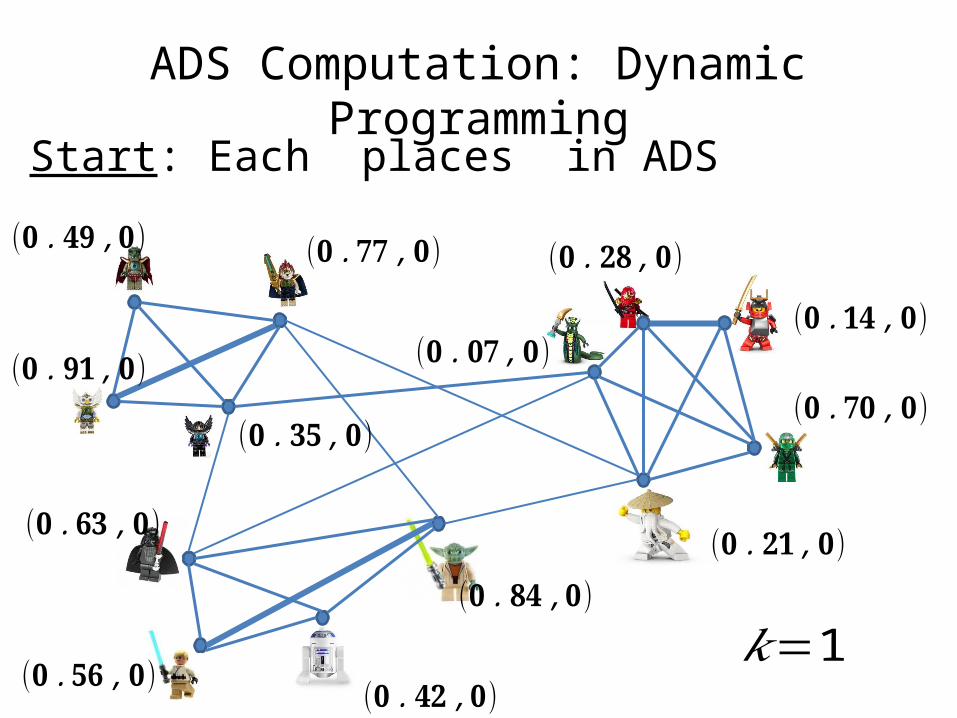
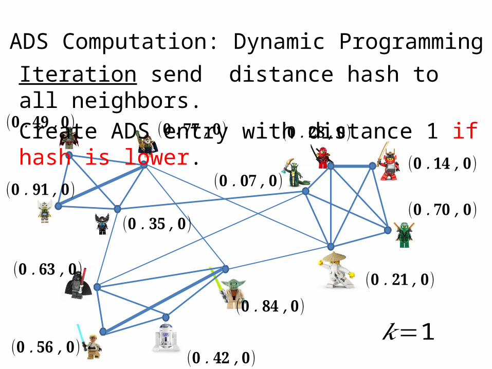
ADS Computation: Dynamic ProgrammingStart: Each places in ADS
𝑘=1
(𝟎 .𝟒𝟗 ,𝟎) (𝟎 .𝟕𝟕 ,𝟎)
(𝟎 .𝟎𝟕 ,𝟎)
(𝟎 .𝟐𝟖 ,𝟎)
(𝟎 .𝟏𝟒 ,𝟎)
(𝟎 .𝟕𝟎 ,𝟎)
(𝟎 .𝟐𝟏 ,𝟎)(𝟎 .𝟖𝟒 ,𝟎)
(𝟎 .𝟗𝟏 ,𝟎)
(𝟎 .𝟑𝟓 ,𝟎)
(𝟎 .𝟔𝟑 ,𝟎)
(𝟎 .𝟓𝟔 ,𝟎) (𝟎 .𝟒𝟐 ,𝟎)
ADS Computation: Dynamic Programming
𝑘=1
(𝟎 .𝟒𝟗 ,𝟎) (𝟎 .𝟕𝟕 ,𝟎)
(𝟎 .𝟎𝟕 ,𝟎)
(𝟎 .𝟐𝟖 ,𝟎)
(𝟎 .𝟏𝟒 ,𝟎)
(𝟎 .𝟕𝟎 ,𝟎)
(𝟎 .𝟐𝟏 ,𝟎)(𝟎 .𝟖𝟒 ,𝟎)
(𝟎 .𝟗𝟏 ,𝟎)
(𝟎 .𝟑𝟓 ,𝟎)
(𝟎 .𝟔𝟑 ,𝟎)
(𝟎 .𝟓𝟔 ,𝟎) (𝟎 .𝟒𝟐 ,𝟎)
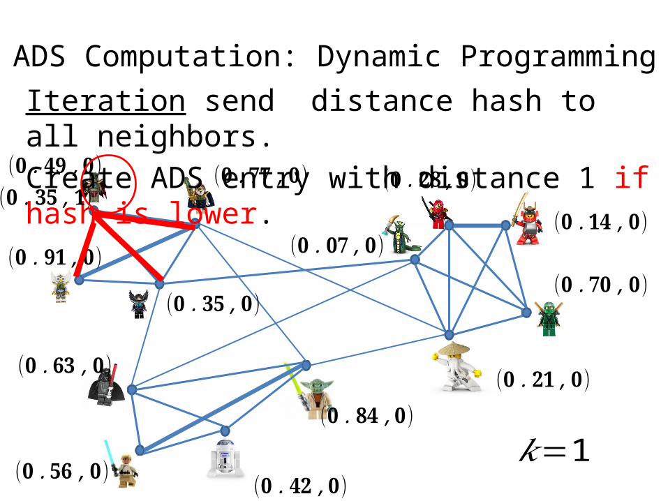
Iteration send distance hash to all neighbors.Create ADS entry with distance 1 if hash is lower.
ADS Computation: Dynamic Programming
𝑘=1
(𝟎 .𝟒𝟗 ,𝟎) (𝟎 .𝟕𝟕 ,𝟎)
(𝟎 .𝟎𝟕 ,𝟎)
(𝟎 .𝟐𝟖 ,𝟎)
(𝟎 .𝟏𝟒 ,𝟎)
(𝟎 .𝟕𝟎 ,𝟎)
(𝟎 .𝟐𝟏 ,𝟎)(𝟎 .𝟖𝟒 ,𝟎)
(𝟎 .𝟗𝟏 ,𝟎)
(𝟎 .𝟑𝟓 ,𝟎)
(𝟎 .𝟔𝟑 ,𝟎)
(𝟎 .𝟓𝟔 ,𝟎) (𝟎 .𝟒𝟐 ,𝟎)
Iteration send distance hash to all neighbors.Create ADS entry with distance 1 if hash is lower.
(𝟎 .𝟑𝟓 ,𝟏)
ADS Computation: Dynamic Programming
𝑘=1
(𝟎 .𝟒𝟗 ,𝟎) (𝟎 .𝟕𝟕 ,𝟎)
(𝟎 .𝟎𝟕 ,𝟎)
(𝟎 .𝟐𝟖 ,𝟎)
(𝟎 .𝟏𝟒 ,𝟎)
(𝟎 .𝟕𝟎 ,𝟎)
(𝟎 .𝟐𝟏 ,𝟎)(𝟎 .𝟖𝟒 ,𝟎)
(𝟎 .𝟗𝟏 ,𝟎)
(𝟎 .𝟑𝟓 ,𝟎)
(𝟎 .𝟔𝟑 ,𝟎)
(𝟎 .𝟓𝟔 ,𝟎) (𝟎 .𝟒𝟐 ,𝟎)
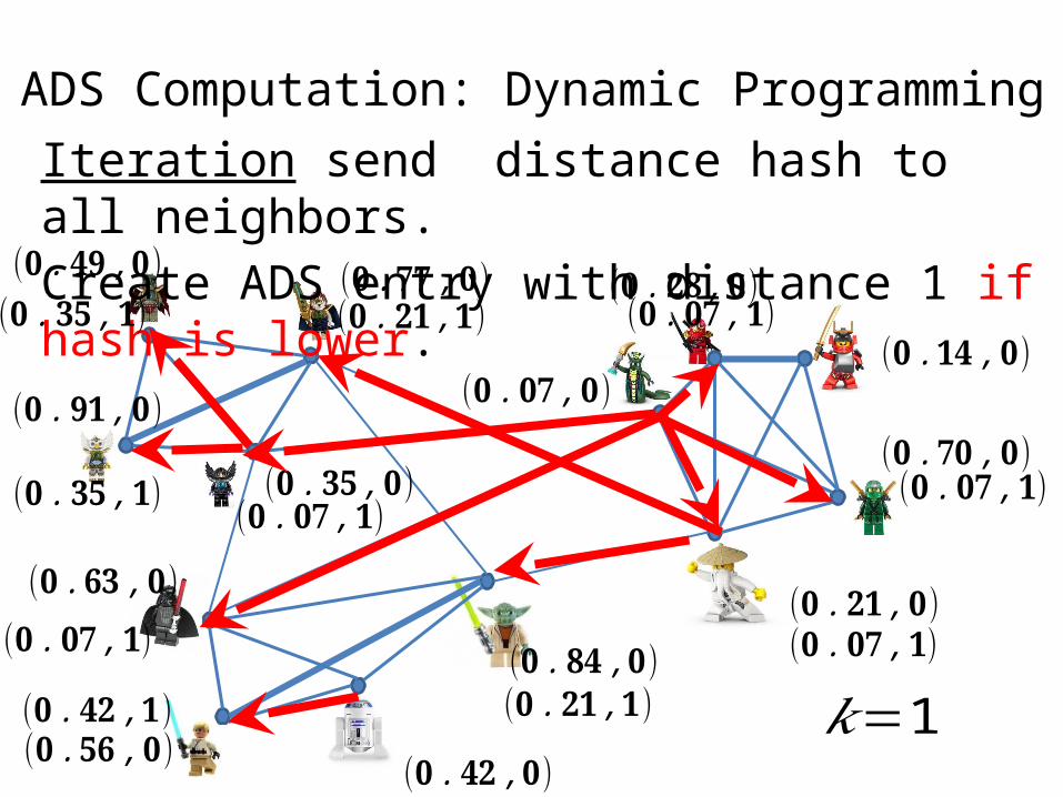
Iteration send distance hash to all neighbors.Create ADS entry with distance 1 if hash is lower.
(𝟎 .𝟑𝟓 ,𝟏)
(𝟎 .𝟑𝟓 ,𝟏) (𝟎 .𝟎𝟕 ,𝟏)
(𝟎 .𝟐𝟏 ,𝟏) (𝟎 .𝟎𝟕 ,𝟏)
(𝟎 .𝟎𝟕 ,𝟏)
(𝟎 .𝟎𝟕 ,𝟏)
(𝟎 .𝟎𝟕 ,𝟏)
(𝟎 .𝟒𝟐 ,𝟏) (𝟎 .𝟐𝟏 ,𝟏)
ADS Computation: Dynamic Programming
𝑘=1
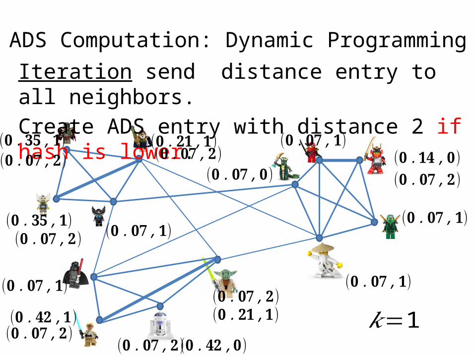
Iteration send distance entry to all neighbors.Create ADS entry with distance 2 if hash is lower.
(𝟎 .𝟑𝟓 ,𝟏)
(𝟎 .𝟑𝟓 ,𝟏) (𝟎 .𝟎𝟕 ,𝟏)
(𝟎 .𝟐𝟏 ,𝟏) (𝟎 .𝟎𝟕 ,𝟏)
(𝟎 .𝟎𝟕 ,𝟏)
(𝟎 .𝟎𝟕 ,𝟏)
(𝟎 .𝟎𝟕 ,𝟏)
(𝟎 .𝟒𝟐 ,𝟏) (𝟎 .𝟐𝟏 ,𝟏)
(𝟎 .𝟎𝟕 ,𝟎)(𝟎 .𝟏𝟒 ,𝟎)
(𝟎 .𝟒𝟐 ,𝟎)
(𝟎 .𝟎𝟕 ,𝟐)
(𝟎 .𝟎𝟕 ,𝟐)
(𝟎 .𝟎𝟕 ,𝟐)(𝟎 .𝟎𝟕 ,𝟐)
(𝟎 .𝟎𝟕 ,𝟐)
(𝟎 .𝟎𝟕 ,𝟐) (𝟎 .𝟎𝟕 ,𝟐)
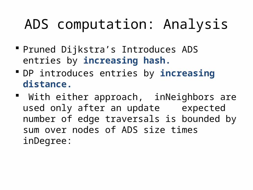
ADS computation: Analysis Pruned Dijkstra’s Introduces ADS entries by
increasing hash. DP introduces entries by increasing distance. With either approach, inNeighbors are used
only after an update expected number of edge traversals is bounded by sum over nodes of ADS size times inDegree:
ADS computation: Comments Pruned Dijkstra ADS computation can be parallelized,
similarly to BFS reachability sketches, to reduce dependency.
DP can be implemented via (diameter number of) sequential passes over edge set. We only need to keep in memory k entries for each node (k smallest hashes so far).
It is also possible to perform a distributed computation where nodes asynchronously communicate with neighbors. Entries can be modified or removed. This incurs overhead.
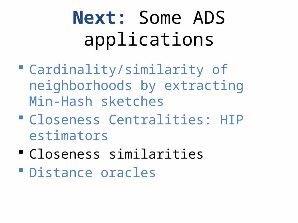
Next: Some ADS applications
Cardinality/similarity of -neighborhoods by extracting Min-Hash sketches
Closeness Centralities: HIP estimators Closeness similarities Distance oracles
Next: Some ADS applications
Cardinality/similarity of -neighborhoods by extracting Min-Hash sketches
Closeness Centralities: HIP estimators Closeness similarities Distance oracles
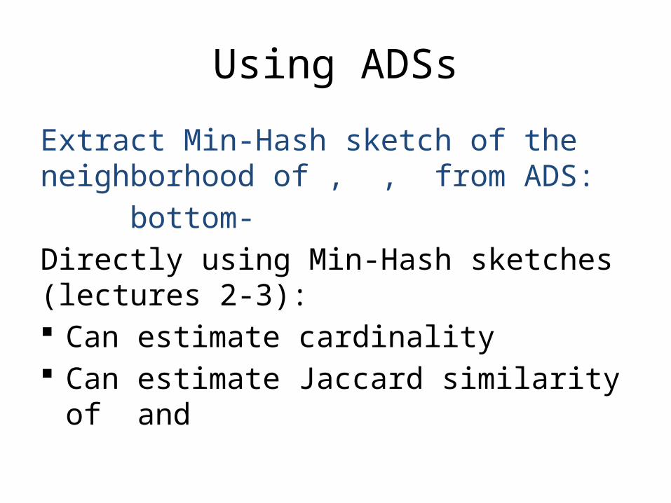
Using ADSs
Extract Min-Hash sketch of the neighborhood of , , from ADS: bottom-Directly using Min-Hash sketches (lectures 2-3): Can estimate cardinality Can estimate Jaccard similarity of and
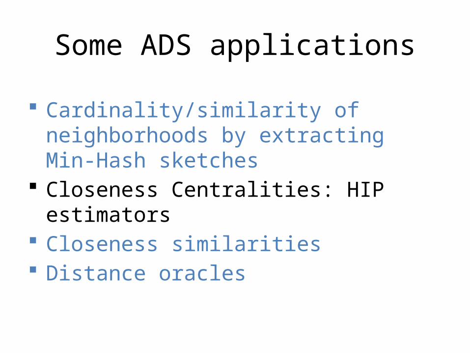
Some ADS applications
Cardinality/similarity of neighborhoods by extracting Min-Hash sketches
Closeness Centralities: HIP estimators Closeness similarities Distance oracles
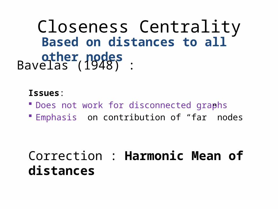
Closeness CentralityBased on distances to all other nodes
Correction : Harmonic Mean of distances
Bavelas (1948) :
Issues: Does not work for disconnected graphs Emphasis on contribution of “far” nodes
Closeness Centrality
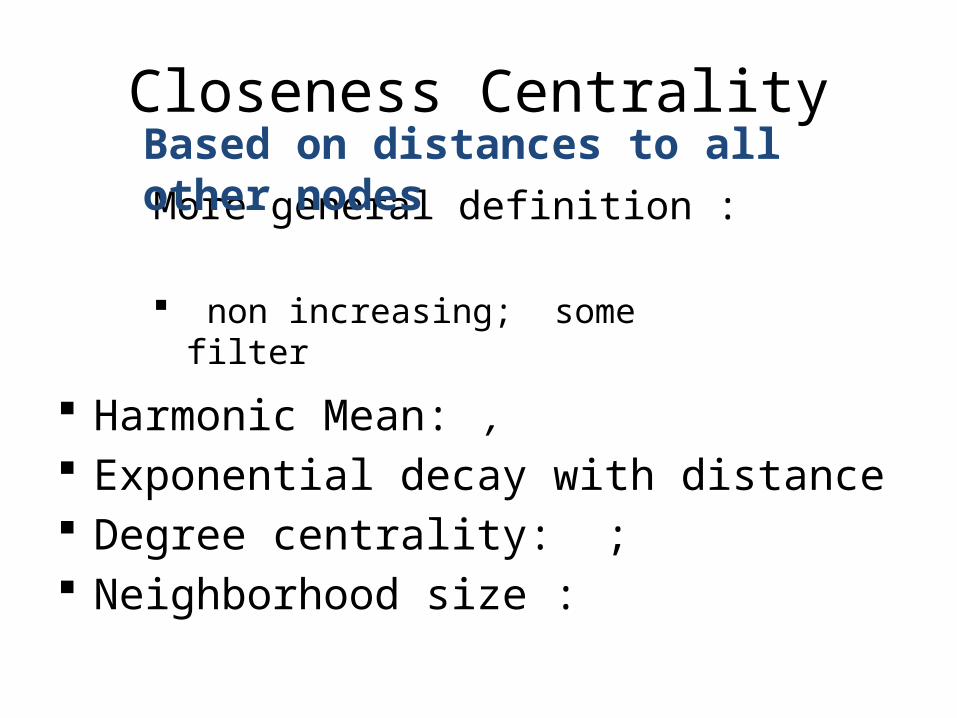
More general definition : non increasing; some filter
Based on distances to all other nodes
Harmonic Mean: , Exponential decay with distance Degree centrality: ; Neighborhood size :
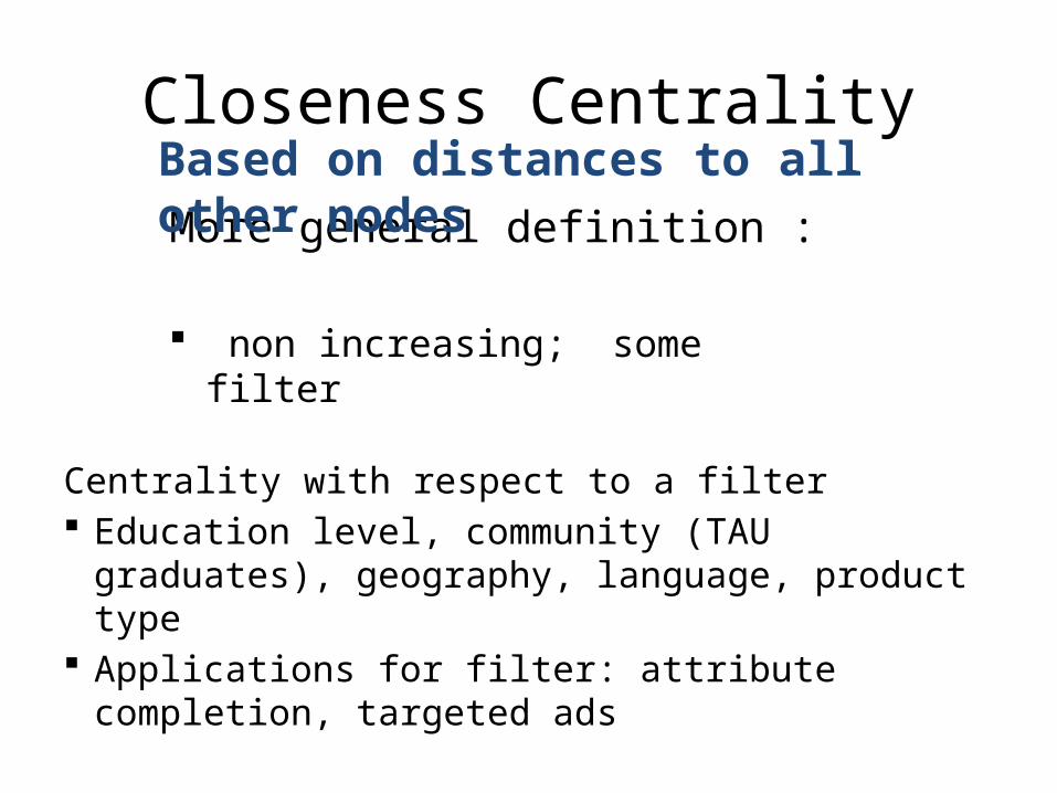
Closeness Centrality
More general definition : non increasing; some filter
Based on distances to all other nodes
Centrality with respect to a filter Education level, community (TAU graduates),
geography, language, product type Applications for filter: attribute completion,
targeted ads
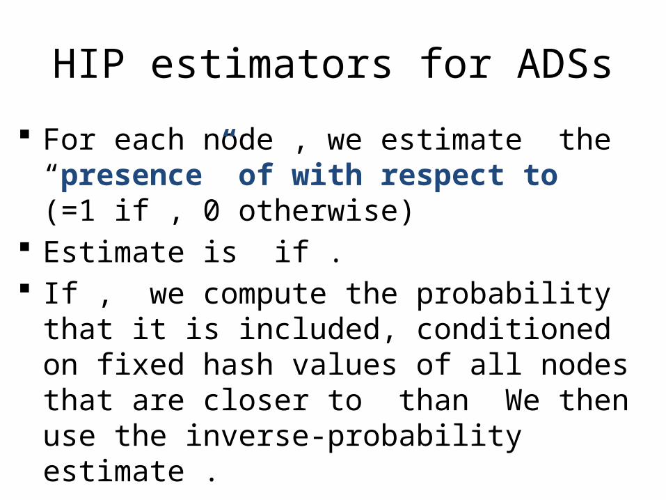
HIP estimators for ADSs
For each node , we estimate the “presence” of with respect to (=1 if , 0 otherwise)
Estimate is if . If , we compute the probability that it is included,
conditioned on fixed hash values of all nodes that are closer to than We then use the inverse-probability estimate .
For bottom- and
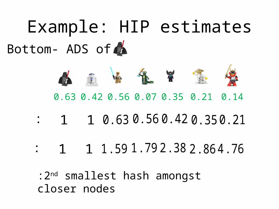
Example: HIP estimates
0.21
Bottom- ADS of
0.63 0.42 0.56 0.07 0.35 0.14
:
:2nd smallest hash amongst closer nodes
11 0.630.56 0.350.210.42
: 11 1.591 .79 2 .864 .762 .38
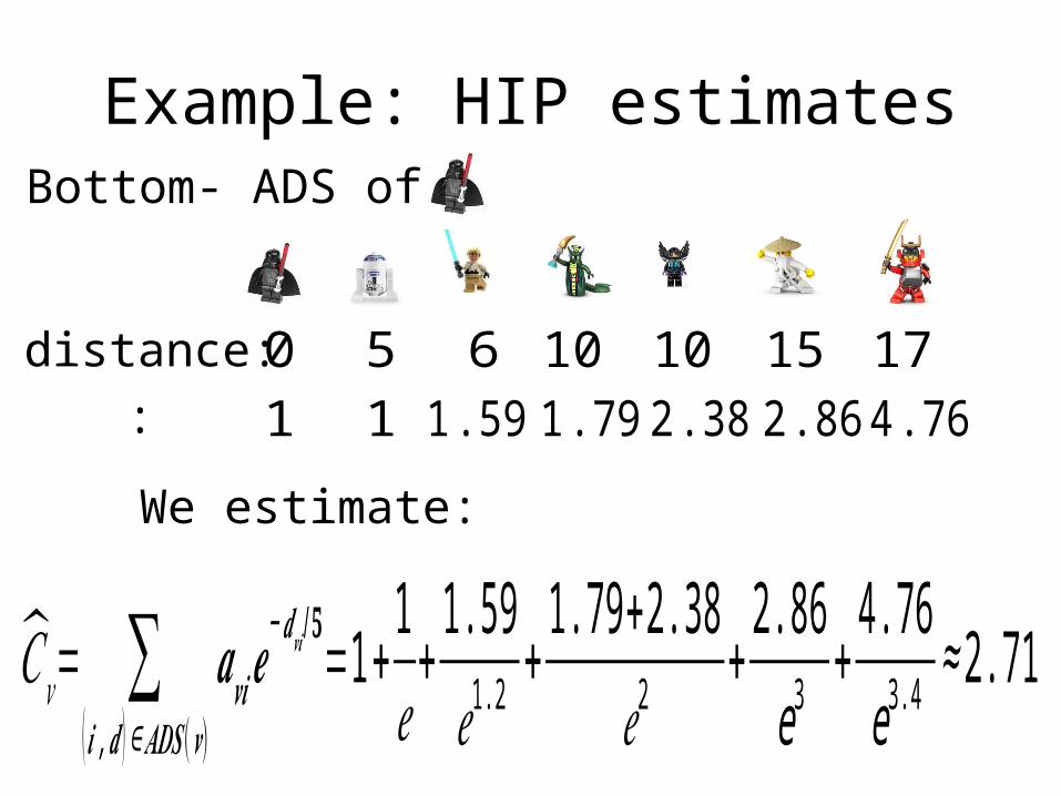
Example: HIP estimatesBottom- ADS of
: 11 1.591 .79 2 .864 .762 .38distance: 50 6 10 15 1710
We estimate:
𝐶𝑣= ∑(𝒊 ,𝒅 )∈𝑨𝑫𝑺 (𝒗)
𝒂𝒗𝒊𝒆−𝒅 𝒗𝒊/𝟓=1+ 1𝑒+1.59𝑒1.2
+1.79+2.38
𝑒2+2.86e3
+4.76e3.4
≈2.71
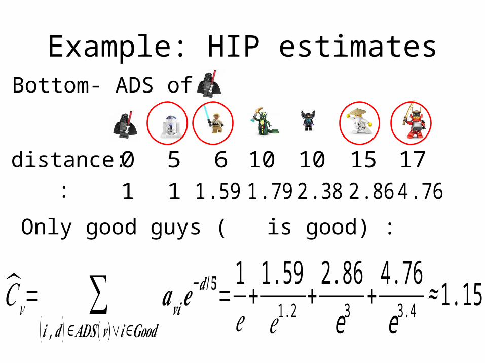
Example: HIP estimatesBottom- ADS of
Only good guys ( is good) :
𝐶𝑣= ∑(𝒊 ,𝒅 )∈𝑨𝑫𝑺 (𝒗)∨ 𝒊∈𝑮𝒐𝒐𝒅
𝒂𝒗𝒊𝒆−𝒅 /𝟓=1𝑒+1.59𝑒1.2
+2.86e3
+4.76e3.4
≈1.15
: 11 1.591 .79 2 .864 .762 .38distance: 50 6 10 15 1710
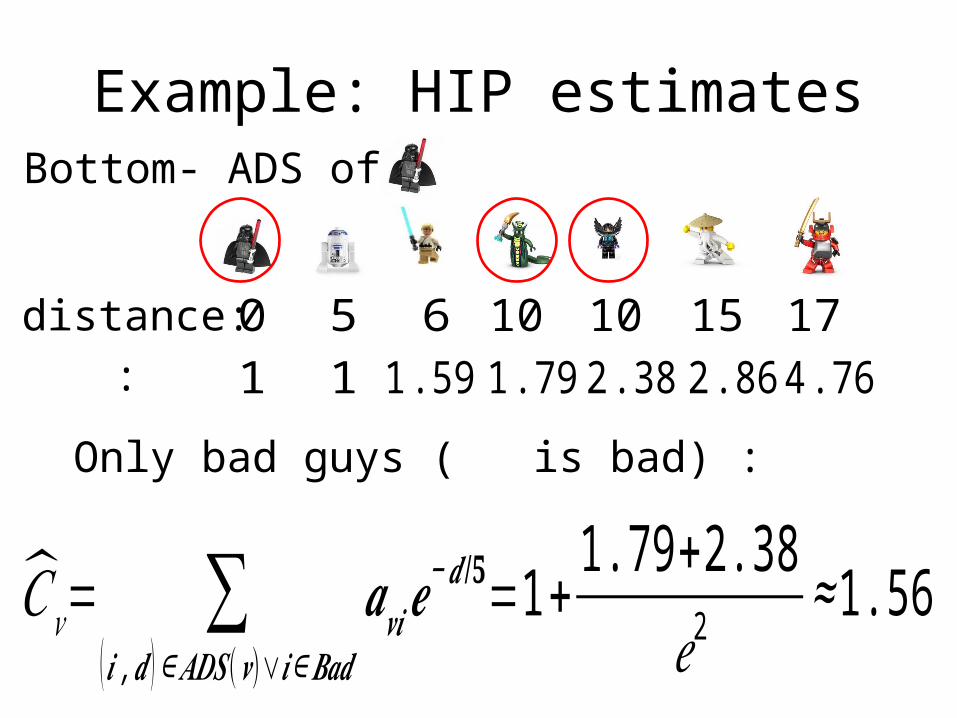
Example: HIP estimatesBottom- ADS of
Only bad guys ( is bad) :
𝐶𝑣= ∑(𝒊 ,𝒅 )∈𝑨𝑫𝑺 (𝒗)∨ 𝒊∈𝑩𝒂𝒅
𝒂𝒗𝒊𝒆−𝒅/𝟓=1+ 1.79+2.38𝑒2
≈1.56
: 11 1.591 .79 2 .864 .762 .38distance: 50 6 10 15 1710
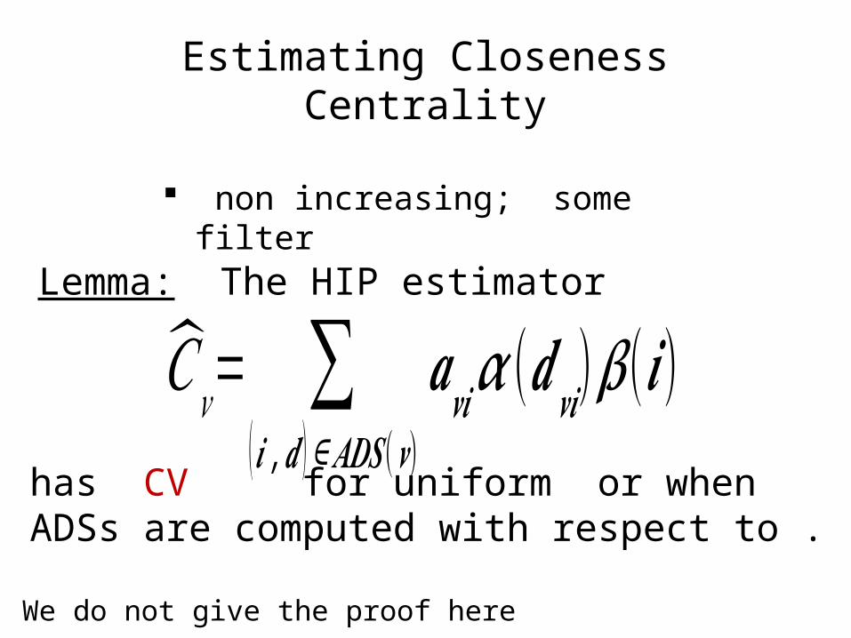
Estimating Closeness Centrality non increasing; some filter
has CV for uniform or when ADSs are computed with respect to .
𝐶𝑣= ∑(𝒊 ,𝒅 )∈𝑨𝑫𝑺 (𝒗)
𝒂𝒗𝒊𝜶 (𝒅𝒗𝒊)𝜷 (𝒊) Lemma: The HIP estimator
We do not give the proof here
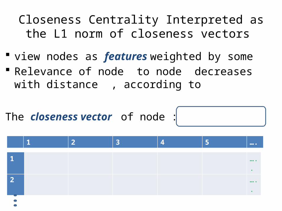
Closeness Centrality Interpreted as the L1 norm of closeness vectors
view nodes as features weighted by some Relevance of node to node decreases with
distance , according to
1 2 3 4 5 ….
2 …..
1 …..
The closeness vector of node :
Next: Some ADS applications
Cardinality/similarity of neighborhoods by extracting Min-Hash sketches
Closeness Centralities: HIP estimators Closeness similarities Distance oracles
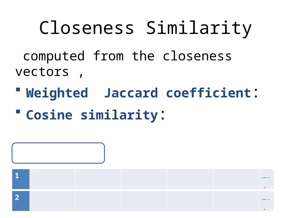
Closeness Similarity computed from the closeness vectors , Weighted Jaccard coefficient: Cosine similarity:
2 …..
1 …..
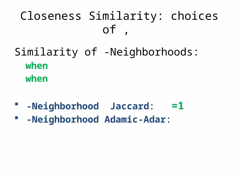
Closeness Similarity: choices of ,
Similarity of -Neighborhoods: when when
-Neighborhood Jaccard: =1 -Neighborhood Adamic-Adar:
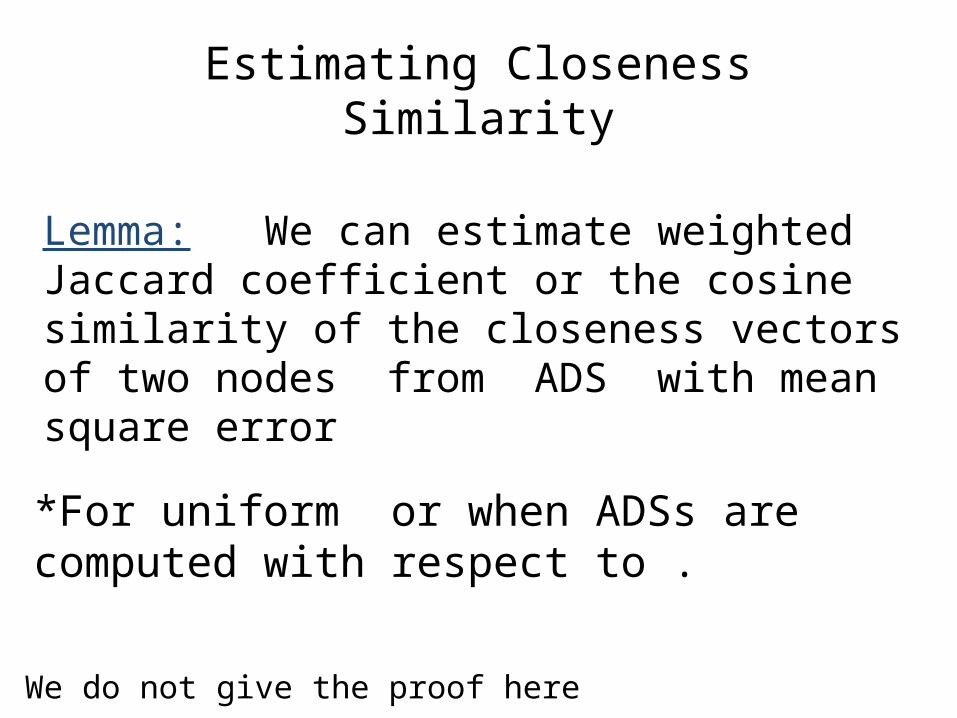
Estimating Closeness Similarity
*For uniform or when ADSs are computed with respect to .
Lemma: We can estimate weighted Jaccard coefficient or the cosine similarity of the closeness vectors of two nodes from ADS with mean square error
We do not give the proof here
Next: Some ADS applications
Cardinality/similarity of neighborhoods by extracting Min-Hash sketches
Closeness Centralities: HIP estimators Closeness similarities Distance oracles
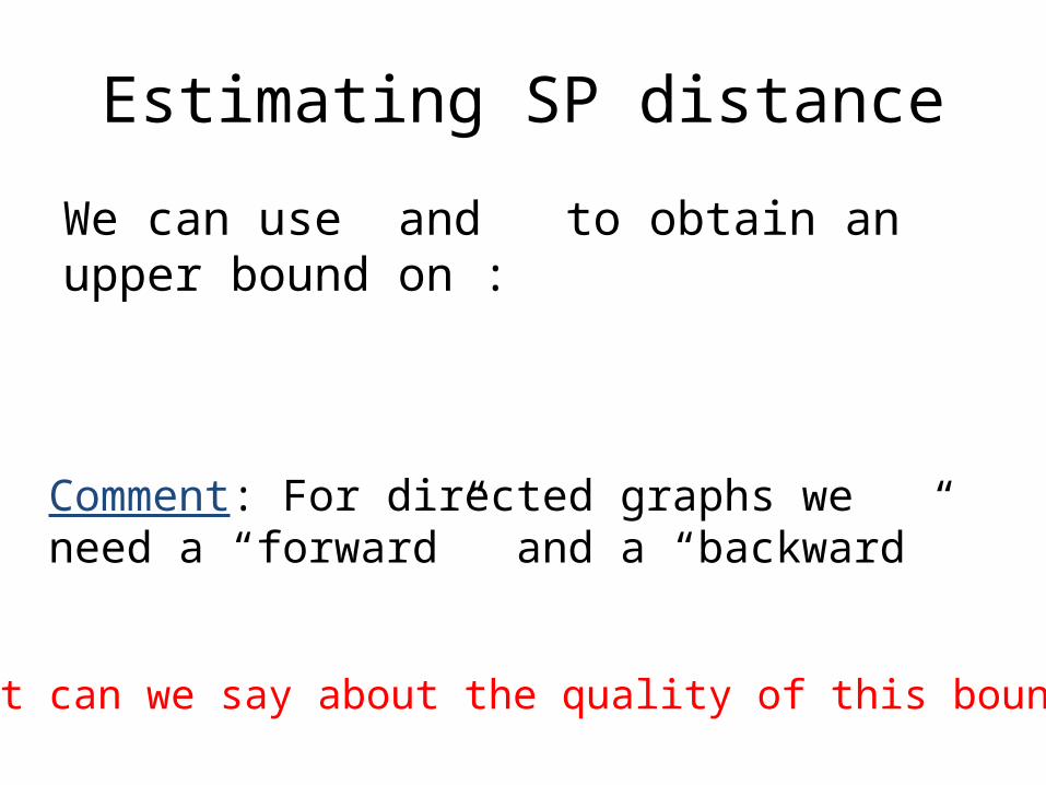
Estimating SP distance
We can use and to obtain an upper bound on :
Comment: For directed graphs we need a “forward” and a “backward”
What can we say about the quality of this bound ?
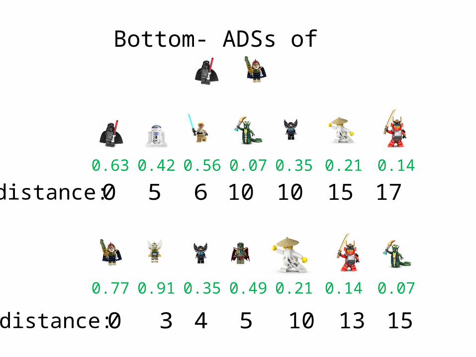
Bottom- ADSs of
0.210.63 0.42 0.56 0.07 0.35 0.14
distance: 50 6 10 15 1710
distance: 30 4 5 13 15100.140.77 0.91 0.35 0.49 0.21 0.07
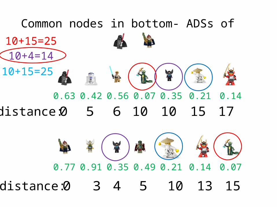
Common nodes in bottom- ADSs of
0.210.63 0.42 0.56 0.07 0.35 0.14
distance: 50 6 10 15 1710
distance: 30 4 5 13 15100.140.77 0.91 0.35 0.49 0.21 0.07
10+15=2510+4=14
10+15=25
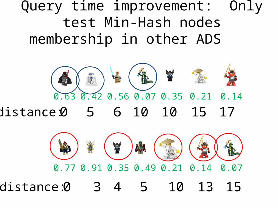
Query time improvement: Only test Min-Hash nodes membership in other ADS
0.210.63 0.42 0.56 0.07 0.35 0.14
distance: 50 6 10 15 1710
distance: 30 4 5 13 15100.140.77 0.91 0.35 0.49 0.21 0.07
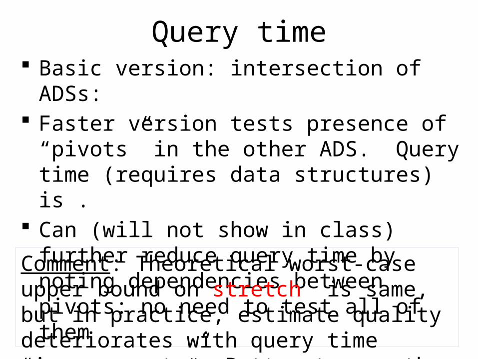
Query time Basic version: intersection of ADSs: Faster version tests presence of “pivots” in the
other ADS. Query time (requires data structures) is .
Can (will not show in class) further reduce query time by noting dependencies between pivots: no need to test all of them
Comment: Theoretical worst-case upper bound on stretch is same, but in practice, estimate quality deteriorates with query time “improvements”: Better to use the full “sketch”
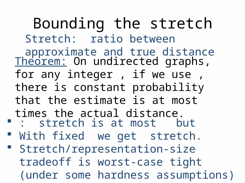
Bounding the stretch
Theorem: On undirected graphs, for any integer , if we use , there is constant probability that the estimate is at most times the actual distance.
: stretch is at most but With fixed we get stretch. Stretch/representation-size tradeoff is worst-case
tight (under some hardness assumptions) In practice, stretch is typically much better.
Stretch: ratio between approximate and true distance
Bounding the stretch
Theorem: On undirected graphs, for any integer , if we use , there is constant probability that the estimate is at most times the actual distance.
We prove a slightly weaker version in class
𝑢 𝑣𝑑
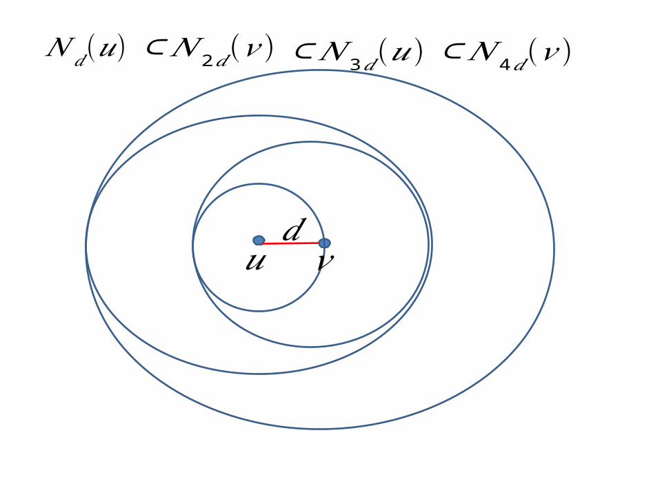
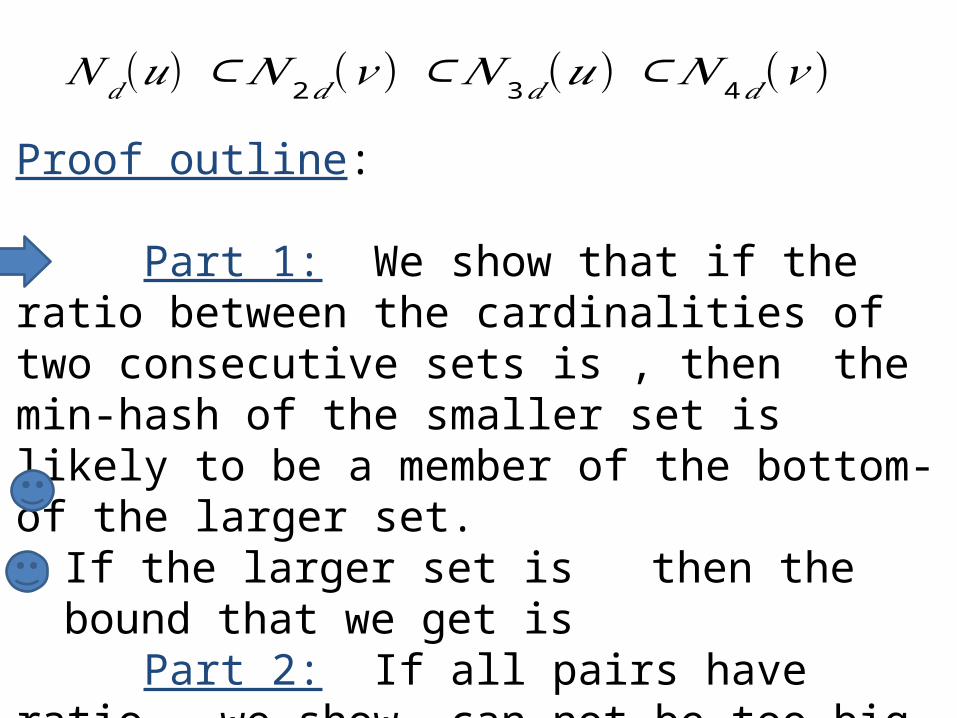
𝑁 𝑑(𝑢)⊂𝑁 2𝑑(𝑣 )⊂𝑁 3𝑑(𝑢)⊂𝑁 4𝑑 (𝑣 )
𝑁 𝑑(𝑢)⊂𝑁 2𝑑(𝑣 )⊂𝑁 3𝑑(𝑢)⊂𝑁 4𝑑 (𝑣 )
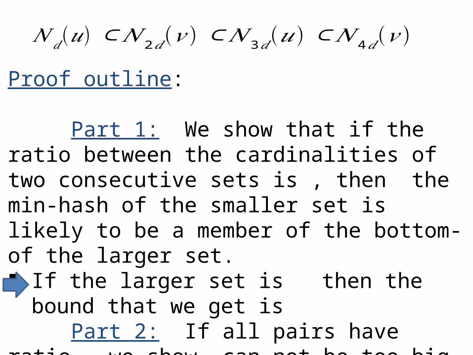
Proof outline:
Part 1: We show that if the ratio between the cardinalities of two consecutive sets is , then the min-hash of the smaller set is likely to be a member of the bottom- of the larger set. If the larger set is then the bound that we get is Part 2: If all pairs have ratio , we show can not be too big and the minimum hash node gives good stretch.
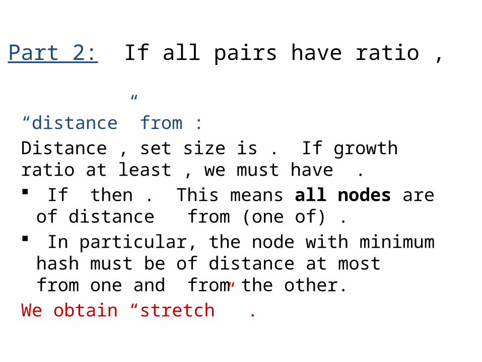
“distance” from : Distance , set size is . If growth ratio at least , we must have . If then . This means all nodes are of distance from
(one of) . In particular, the node with minimum hash must be
of distance at most from one and from the other.We obtain “stretch” .
Part 2: If all pairs have ratio ,
𝑁 𝑑(𝑢)⊂𝑁 2𝑑(𝑣 )⊂𝑁 3𝑑(𝑢)⊂𝑁 4𝑑 (𝑣 )
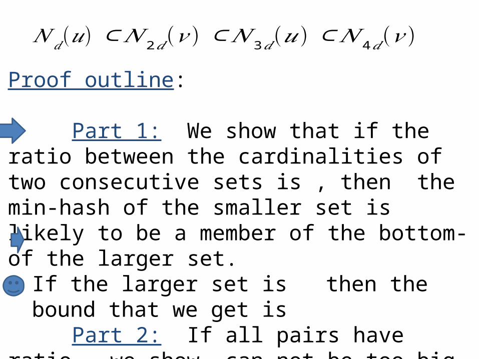
Proof outline:
Part 1: We show that if the ratio between the cardinalities of two consecutive sets is , then the min-hash of the smaller set is likely to be a member of the bottom- of the larger set. If the larger set is then the bound that we get is Part 2: If all pairs have ratio , we show can not be too big and the minimum hash node gives good stretch.
𝑢 𝑣𝑑
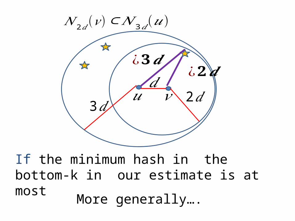
𝑁 2𝑑(𝑣 )⊂𝑁 3𝑑(𝑢)
If the minimum hash in the bottom-k in our estimate is at most
2𝑑3𝑑
More generally….
¿𝟐𝒅¿𝟑𝒅
𝑢 𝑣𝑑
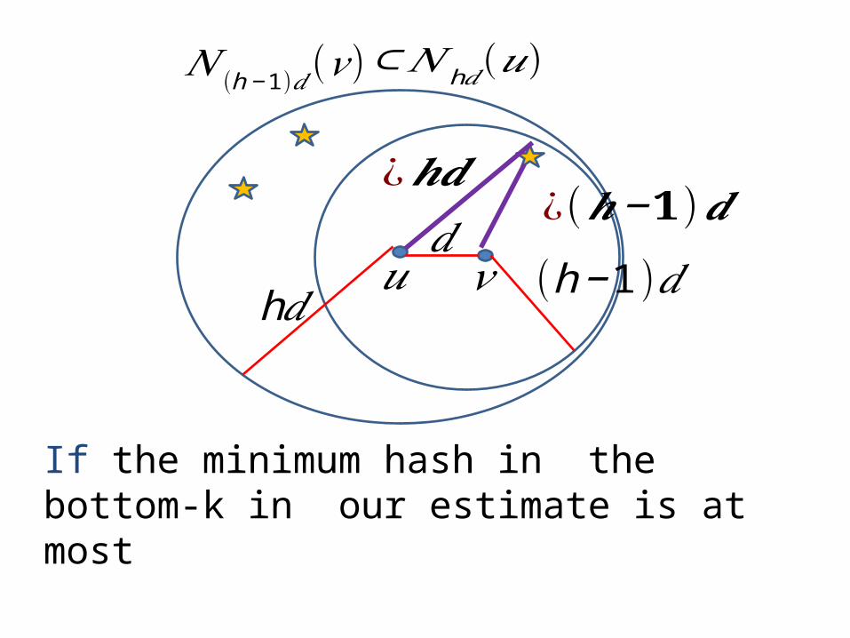
𝑁 (h−1)𝑑(𝑣)⊂𝑁 h𝑑(𝑢)
If the minimum hash in the bottom-k in our estimate is at most
(h−1)𝑑h𝑑
¿ (𝒉−𝟏)𝒅¿𝒉𝒅
𝑁 𝑑(𝑢)⊂𝑁 2𝑑(𝑣 )⊂𝑁 3𝑑(𝑢)⊂𝑁 4𝑑 (𝑣 )
Proof outline:
Part 1: We show that if the ratio between the cardinalities of two consecutive sets is , then the min-hash of the smaller set is likely to be a member of the bottom- of the larger set. If the larger set is then the bound that we get is Part 2: If all pairs have ratio , we show can not be too big and the minimum hash node gives good stretch.
𝑢 𝑣𝑑
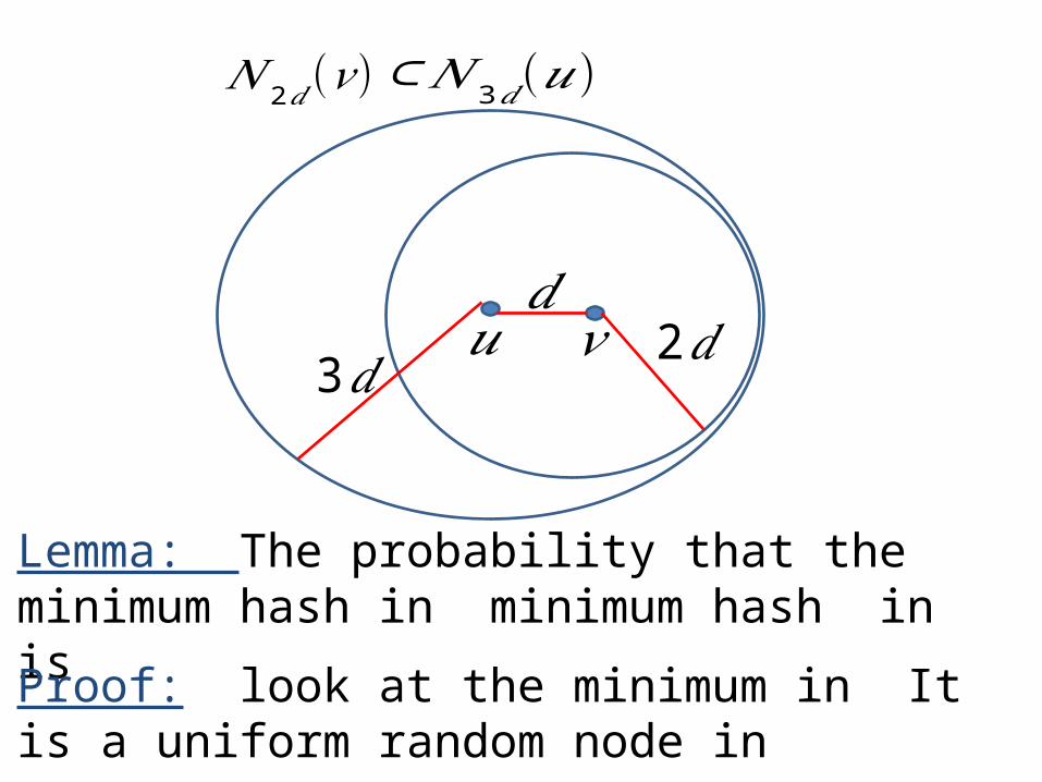
𝑁 2𝑑(𝑣 )⊂𝑁 3𝑑(𝑢)
Lemma: The probability that the minimum hash in minimum hash in is
2𝑑3𝑑
Proof: look at the minimum in It is a uniform random node in
𝑁 2𝑑(𝑣 )⊂𝑁 3𝑑(𝑢)
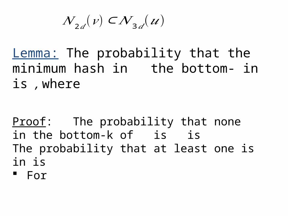
Lemma: The probability that the minimum hash in the bottom- in is , where Proof: The probability that none in the bottom-k of is is The probability that at least one is in is For
𝑁 2𝑑(𝑣 )⊂𝑁 3𝑑(𝑢)
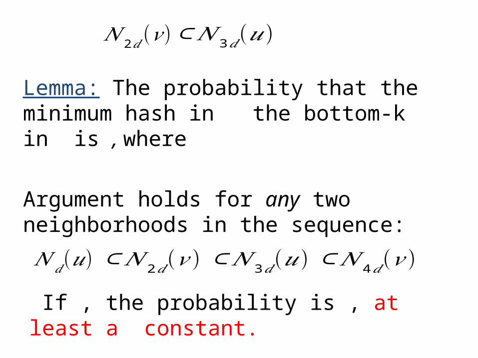
Lemma: The probability that the minimum hash in the bottom-k in is , where Argument holds for any two neighborhoods in the sequence:
𝑁 𝑑(𝑢)⊂𝑁 2𝑑(𝑣 )⊂𝑁 3𝑑(𝑢)⊂𝑁 4𝑑 (𝑣 )
If , the probability is , at least a constant.
Bibliography Closeness centrality on ADSs using HIP: E. Cohen “All-Distances
Sketches, Revisited: HIP Estimators for Massive Graphs Analysis” arXiv 2013
Closeness similarity and distance oracles using ADSs: E. Cohen, D. Delling, F. Fuchs, A. Goldberg,M. Goldszmidt, and R. Werneck. “Scalable similarity estimation in social networks: Closeness, node labels, and random edge lengths.” In COSN, 2013.
Related: Distance distribution on social graphs: P. Boldi, M. Rosa, and S. Vigna.
HyperANF: “approximating the neighbourhood function of very large graphs on a budget.” In WWW, 2011
More on distance oracles: M. Thorup U. Zwick “Approximate Distance Oracles” JACM 2005
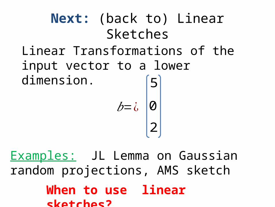
Next: (back to) Linear SketchesLinear Transformations of the input vector to a lower dimension.
2𝑏=¿05
When to use linear sketches?
Examples: JL Lemma on Gaussian random projections, AMS sketch
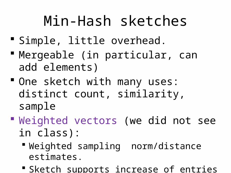
Min-Hash sketches Simple, little overhead. Mergeable (in particular, can add elements) One sketch with many uses: distinct count,
similarity, sample Weighted vectors (we did not see in class):
Weighted sampling norm/distance estimates. Sketch supports increase of entries values or
replace with a larger value.But.. no support for negative updates
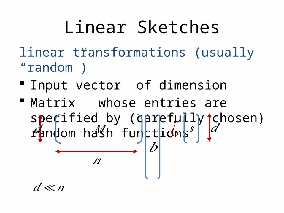
Linear Sketcheslinear transformations (usually “random”) Input vector of dimension Matrix whose entries are specified by
(carefully chosen) random hash functions
𝑀𝑏¿ 𝑠𝑑 𝑑
𝑛
𝑑≪𝑛
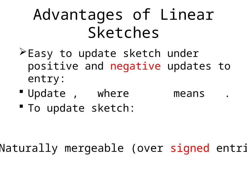
Advantages of Linear Sketches
Easy to update sketch under positive and negative updates to entry:
Update , where means . To update sketch:
Naturally mergeable (over signed entries)
Recommended

![Accumulo Summit 2015: Event-Driven Big Data with Accumulo - Leveraging Big Data in Motion [Leveraging Accumulo]](https://img.pdfslide.us/doc/110x75/55a5e4371a28ab32368b476f/accumulo-summit-2015-event-driven-big-data-with-accumulo-leveraging-big-data-in-motion-leveraging-accumulo.jpg)