Lecture (chapter 10):Hypothesis testing III:
The analysis of varianceErnesto F. L. Amaral
March 19–21, 2018Advanced Methods of Social Research (SOCI 420)
Source: Healey, Joseph F. 2015. ”Statistics: A Tool for Social Research.” Stamford: Cengage Learning. 10th edition. Chapter 10 (pp. 247–275).

Chapter learning objectives• Identify and cite examples of situations in which analysis
of variance (ANOVA) is appropriate
• Explain the logic of hypothesis testing as applied to ANOVA
• Perform the ANOVA test, using the five-step model as a guide, and correctly interpret the results
• Define and explain the concepts of population variance, total sum of squares, sum of squares between, sum of squares within, mean square estimates
• Explain the difference between the statistical significance and the importance (magnitude) of relationships between variables
2

ANOVA application• ANOVA can be used in situations where the
researcher is interested in the differences in sample means across three or more categories
– How do Protestants, Catholics, and Jews vary in terms of number of children?
– How do Republicans, Democrats, and Independents vary in terms of income?
– How do older, middle-aged, and younger people vary in terms of frequency of church attendance?
3

Extension of t-test• We can think of ANOVA as an extension of t-test
for more than two groups– Are the differences between the samples large
enough to reject the null hypothesis and justify the conclusion that the populations represented by the samples are different?
• Null hypothesis, H0
– H0: μ1 = μ2= μ3 = … = μk
– All population means are similar to each other
• Alternative hypothesis, H1
– At least one of the populations means is different4
• Could there be a relationship between age and support for capital punishment?– No difference between groups
– Difference between groups
Logic of ANOVA
5Source: Healey 2015, p.249.

Between and within differences• If the H0 is true, the sample means should be
about the same value– If the H0 is true, there will be little difference between
sample means
• If the H0 is false– There should be substantial differences between
sample means (between categories)– There should be relatively little difference within
categories• The sample standard deviations should be small within
groups
6

Likelihood of rejecting H0• The greater the difference between categories
(as measured by the means)– Relative to the differences within categories (as
measured by the standard deviations)– The more likely the H0 can be rejected
• When we reject H0– We are saying there are differences between the populations represented by the sample
7
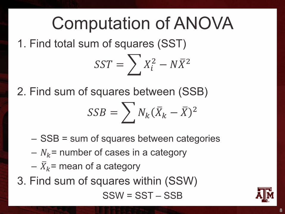
Computation of ANOVA1. Find total sum of squares (SST)
!!" =$%&' − ) *%'
2. Find sum of squares between (SSB)
!!+ =$), *%, − *% '
– SSB = sum of squares between categories– ),= number of cases in a category– *%,= mean of a category
3. Find sum of squares within (SSW)SSW = SST – SSB
8

4. Degrees of freedomdfw = N – k
– dfw = degrees of freedom within– N = total number of cases– k = number of categories
dfb = k – 1– dfb = degrees of freedom between– k = number of categories
9

Final estimations5. Find mean square estimates
!"#$ %&'#(" )*+ℎ*$ = ../01)
!"#$ %&'#(" 2"+)""$ = ..3012
6. Find the F ratio
4 52+#*$"0 = !"#$ %&'#(" 2"+)""$!"#$ %&'#(" )*+ℎ*$
10

Example• Support for capital punishment• Sample of 16 people who are equally divided
across four age groups
11Source: Healey 2015, p.252.

Step 1: Assumptions,requirements• Independent random samples
• Interval-ratio level of measurement
• Normally distributed populations
• Equal population variances
12

Step 2: Null hypothesis• Null hypothesis, H0: μ1 = μ2 = μ3 = μ4
– The null hypothesis asserts there is no difference between the populations
• Alternative hypothesis, H1– At least one of the populations means is different
13

Step 3: Distribution, critical region• Sampling distribution
– F distribution
• Significance level– Alpha (α) = 0.05
• Degrees of freedom– dfw = N – k = 16 – 4 = 12– dfb = k – 1 = 4 – 1 = 3
• Critical F– F(critical) = 3.49
14
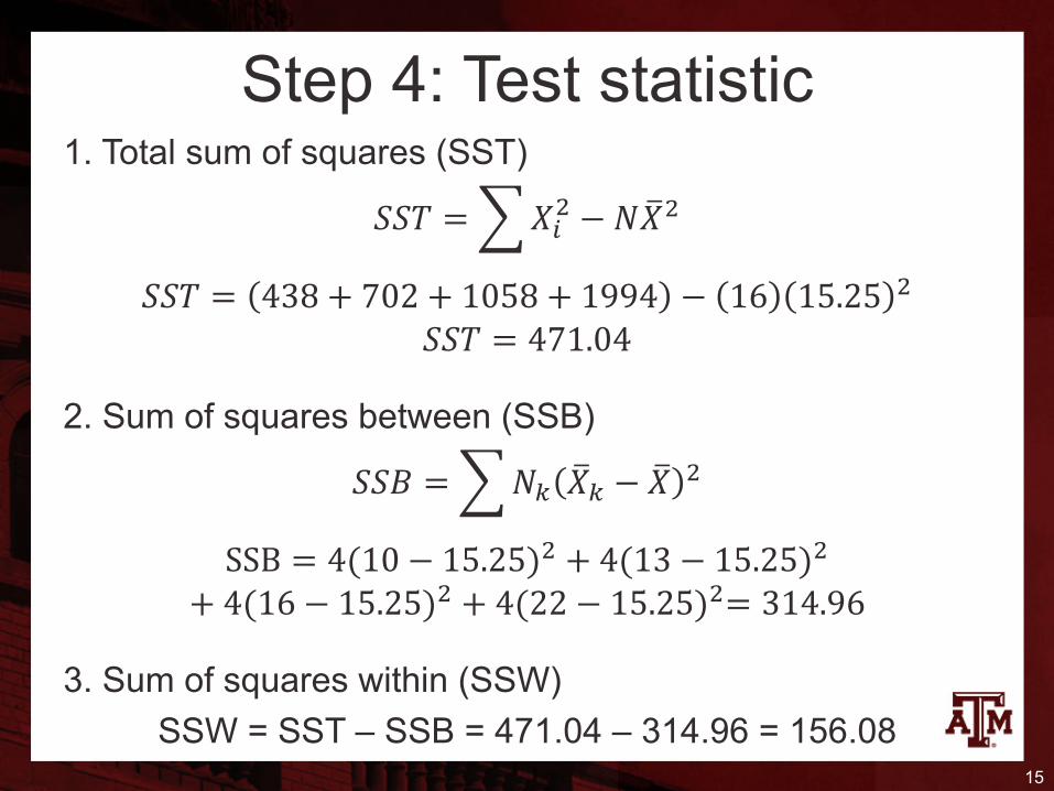
1. Total sum of squares (SST)
!!" =$%&' − ) *%'
!!" = 438 + 702 + 1058 + 1994 − 16 15.25 '
!!" = 471.04
2. Sum of squares between (SSB)
!!7 =$)8 *%8 − *% '
SSB = 4(10 − 15.25)' + 4(13 − 15.25)'+ 4(16 − 15.25)' + 4(22 − 15.25)'= 314.96
3. Sum of squares within (SSW)SSW = SST – SSB = 471.04 – 314.96 = 156.08
15
Step 4: Test statistic

4. Degrees of freedomdfw = N – k = 16 – 4 = 12
dfb = k – 1 = 4 – 1 = 3
5. Mean square estimates
!"#$ %&'#(" )*+ℎ*$ = ../01) = 156.08
12 = 13.00
!"#$ %&'#(" :"+)""$ = ..;01: =
314.963 = 104.99
6. F ratio
> ?:+#*$"0 = !"#$ %&'#(" :"+)""$!"#$ %&'#(" )*+ℎ*$ = 104.99
13.00= 8.08
16
Step 5: Decision, interpret
17
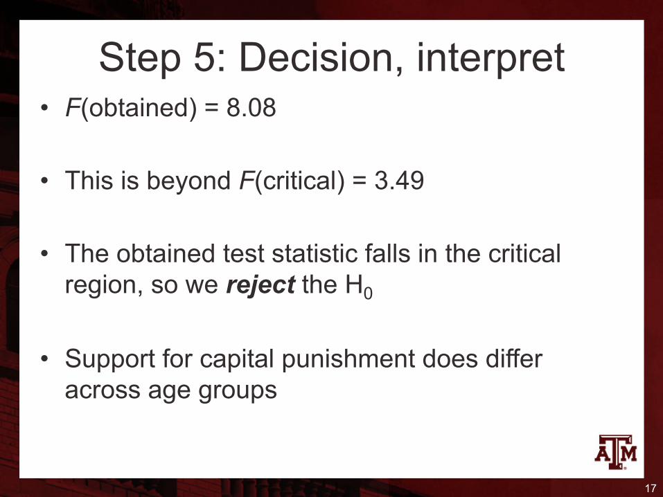
• F(obtained) = 8.08
• This is beyond F(critical) = 3.49
• The obtained test statistic falls in the critical region, so we reject the H0
• Support for capital punishment does differ across age groups

• We know the average income by race/ethnicity
• Does at least one category of the race/ethnicity variable have average income different than the others?– This is not a perfect example for ANOVA, because the
race/ethnicity variable does not have equal numbers of cases across its categories
Example from 2016 GSS
18
Other 50156.34855 59219.9 72 Hispanic 23128.91777 21406.31 215 Black 23243.0413 19671.53 273 White 38845.61946 39157.17 1,072 icity mean(conrinc) sd(conrinc) N(conrinc)Race/Ethn
. table raceeth [aweight=wtssall], c(mean conrinc sd conrinc n conrinc)

• The probability of not rejecting H0 is small (p<0.01)– At least one category of the race/ethnicity variable has average
income different than the others with a 99% confidence level– However, ANOVA does not inform which category has an
average income significantly different than the others in 2016
Example from GSS: Result
19
Total 2.1994e+12 1631 1.3485e+09 Within groups 2.0980e+12 1628 1.2887e+09Between groups 1.0142e+11 3 3.3806e+10 26.23 0.0000 Source SS df MS F Prob > F Analysis of Variance
. oneway conrinc raceeth [aweight=wtssall]
Source: 2016 General Social Survey.
Edited table
20
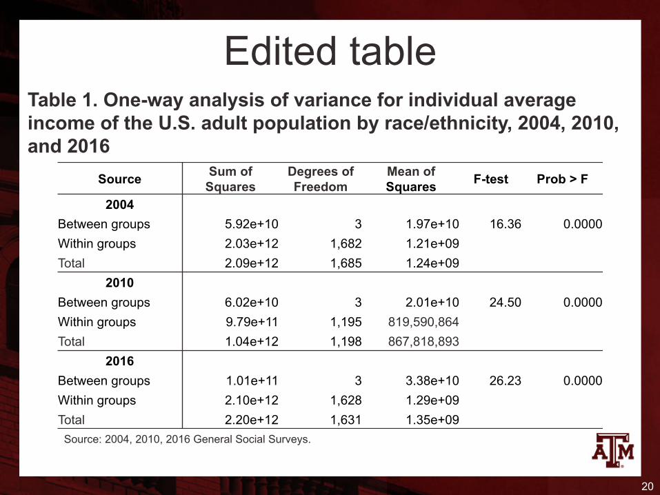
Source: 2004, 2010, 2016 General Social Surveys.
Table 1. One-way analysis of variance for individual average income of the U.S. adult population by race/ethnicity, 2004, 2010, and 2016
Source Sum ofSquares
Degrees ofFreedom
Mean ofSquares F-test Prob > F
2004Between groups 5.92e+10 3 1.97e+10 16.36 0.0000Within groups 2.03e+12 1,682 1.21e+09Total 2.09e+12 1,685 1.24e+09
2010Between groups 6.02e+10 3 2.01e+10 24.50 0.0000Within groups 9.79e+11 1,195 819,590,864Total 1.04e+12 1,198 867,818,893
2016Between groups 1.01e+11 3 3.38e+10 26.23 0.0000Within groups 2.10e+12 1,628 1.29e+09Total 2.20e+12 1,631 1.35e+09

Limitations of ANOVA• Requires interval-ratio level measurement of the
dependent variable• Requires roughly equal numbers of cases in the
categories of the independent variable• Statistically significant differences are not
necessarily important (small magnitude)• The alternative (research) hypothesis is not
specific– It only asserts that at least one of the population
means differs from the others
21

Recommended